Time Scale Effects and Interactions of Rainfall Erosivity and Cover Management Factors on Vineyard Soil Loss Erosion in the Semi-Arid Area of Southern Sicily

Abstract

Several authors describe the effectiveness of cover crop management practice as an important tool to prevent soil erosion, but at the same time, they stress on the high soil loss variability due to the interaction of several factors characterized by large uncertainty. In this paper the Revised Universal Soil Loss Equation (RUSLE) model is applied to two Sicilian vineyards that are characterized by different topographic factors; one is subjected to Conventional Practice (CP) and the other to Best Management Practice (BMP). By using climatic input data at a high temporal scale resolution for the rainfall erosivity (R) factor, and remotely sensed imagery for the cover and management (C) factor, the importance of an appropriate R and C factor assessment and their inter and intra-annual interactions in determining soil erosion variability are showed. Different temporal analysis at ten-year, seasonal, monthly and event scales showed that results at events scales allow evidencing the interacting factors that determine erosion risk features which at other temporal scales of resolution can be hidden. The impact of BMP in preventing soil erosion is described in terms of average saved soil loss over the 10-year period of observation. The evaluation of soil erosion at a different temporal scale and its implications can help stakeholders and scientists formulate better soil conservation practices and agricultural management, and also consider that erosivity rates are expected to raise for the increase of rainfall intensity linked to climate change.

1. Introduction

Soil erosion in vineyards represent several environmental issues. In the semi-arid environment, where the soil is maintained bare, to limit water competition with weeds and rainfall trend is variable and considerable mainly in the winter period, protective practices are also supported from an economic point of view both for soil erosion control and soil organic matter improvement.

Commonly, the Revised Universal Soil Loss Equation (RUSLE) and its family of models have been widely applied in order to evaluate the soil erosion risk [1]. The RUSLE model integrates a number of sub-factors describing the main components of the erosion processes, including rainfall erosivity, soil erodibility, topographic factors, and cover and practices management.

Very important information about rainfall erosivity, which in the RUSLE approach is considered by the R sub-factor, is the time or month of the year when erosivity is at its maximum as well as when it is at its minimum, but also its variability within the considered time or period. The high level of risk linked to the well-known uncertainty of rainfall events allows us to mainly consider the probability of erosivity events.

Despite several studies highlighting that in the semi-arid environment the rainfall intensity is higher in winter or autumn [2,3,4,5], in Sicily, D’Asaro et al. [6] estimated the summer erosivity to be equal to or slightly higher than the winter one. The same intensity of rainfall erosivity can result in more or less effectiveness on soil erosion according to the time of year when it occurs depending on different factors, like crop cover, that change during the year. Therefore, knowledge about the time of year when the highest erosivity occurs is critical for management practices, as it allows to optimize mitigation and adaptation procedures. But for these reasons, also probability of the cover factor in the same period or month of the erosivity factor, must be taken into account together with its occurrence probability.

At the same time, a high erosivity factor can occur together with an excellent crop or residue cover not affecting soil erosion processes. On the contrary, serious problems result if a bare soil period matches with a sporadic high erosivity event.

The best management practices (BMP) aimed at soil erosion control use cover cropping as the main tool to achieve the goal, but the presence of soil covering is affected by a high intra-annual and inter-annual variability due to climatic and environmental factors (seedling date, emergence, drought during spring and cover crops burying period, etc.).

In the RUSLE model, the inter-annual variability of crop management is described by the C factor. In particular, the C factor monthly variability needs to be accounted for. At this aim, the potentiality of remote sensing can be exploited using the well-known Normalized Difference Vegetation Index (NDVI) estimated from time-series satellite imagery. NDVI quantifies vegetation by measuring the difference between near-infrared (which vegetation strongly reflects) and red radiation (which vegetation absorbs). In particular, using data from the Moderate Resolution Imaging Spectroradiometer (MODIS), the National Aeronautics and Space Administration Earth Observing System (NASA/EOS) produced a global dataset of NDVI time-series at 8 and 16-day time steps and characterized by a pixel resolutions ranging from 250–1000 m, which can be easily retrieved from the Land Processes Distributed Active Archive Center [7]. The inter-annual variability of observed NDVI can be transformed in a corresponding C factor variability using one of the various approaches proposed in literature through regression correlation analysis [8,9,10].

According to Panagos [11], monthly erosivity probability allows imposing and/or recommend sustainable agricultural management practices (crop residues, reduced tillage) in regions with high erosivity probability.

If the spatiotemporal rainfall erosivity analysis is a first step towards developing dynamic maps of soil loss by water erosion, the same approach must be applied to the other factor characterized by inter-annual and intra-annual variability such as the cover factor. For these reasons, the distribution over time of the factors involved in the RUSLE equation (R and C factor) must be known. Additionally, their interaction with the goal to identify the riskiest period.

The consequent study of probability is important to support flood prevention, hazard mitigation, ecosystem services, land use change, agricultural production and food security, in general.

For the reasons in this paper, the interactions of rainfall erosivity and cover management factors, as well as their time scale effects, for the vineyard crop, were studied. In particular, the following main objectives of the research were pursued:

(i)

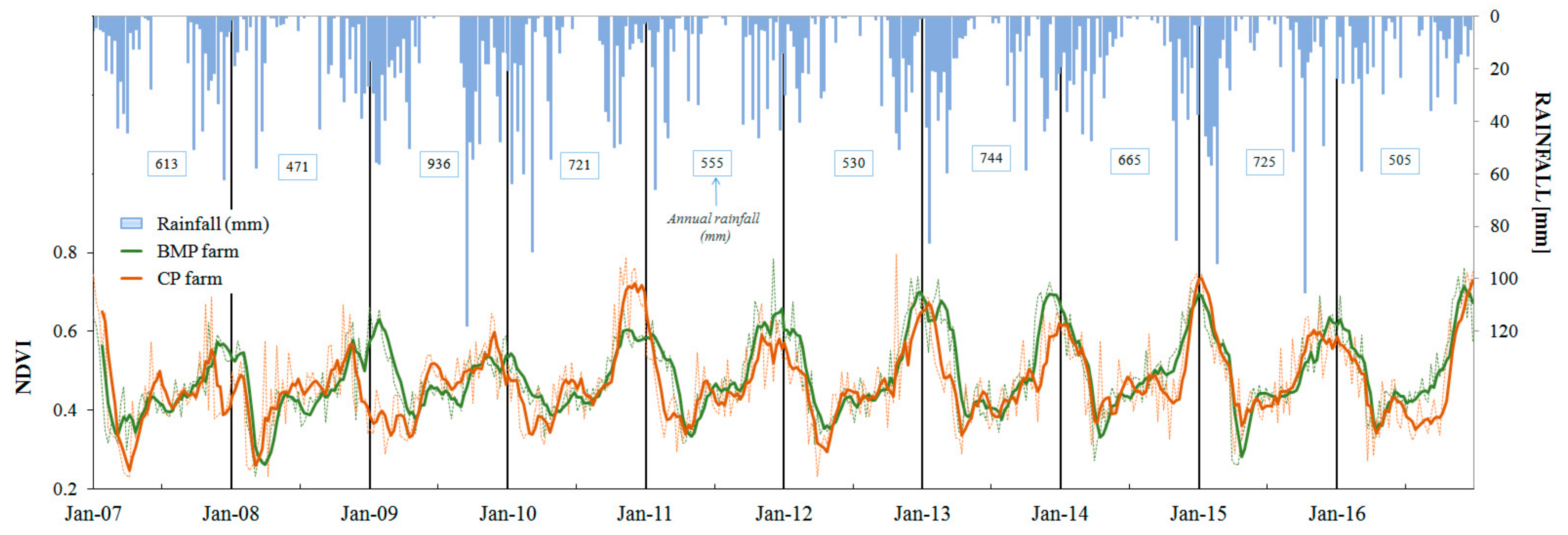
Modeling inter-annual variability of C factor using time-series products of NDVI provided by MODIS satellite platform;

(ii)

Assessing the importance of monthly C and R factors and their temporal interactions in comparison to the corresponding annual values, and;

(iii)

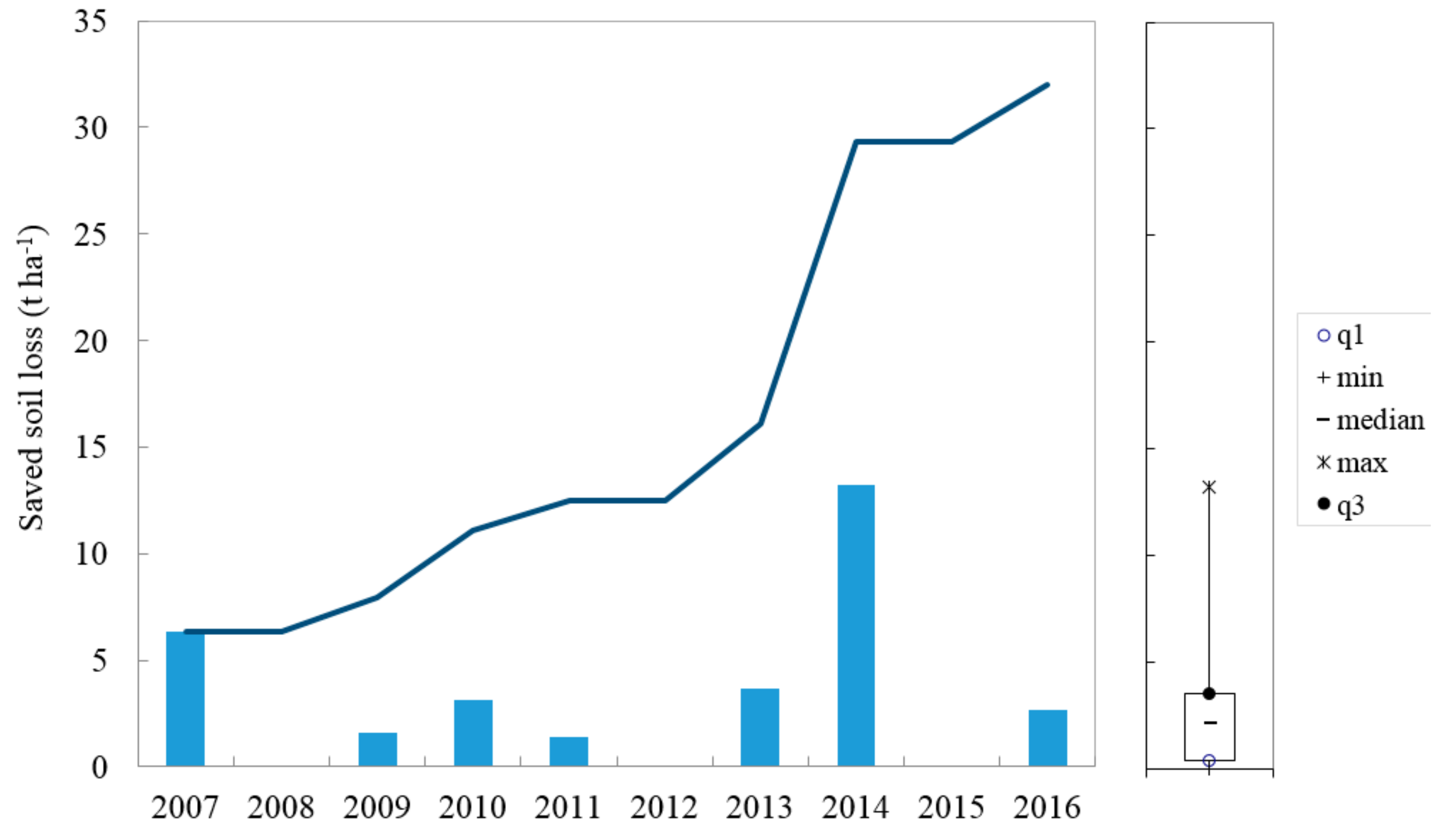
Assessing soil erosion risk in relation to BMP adoption in the semi-arid vineyard.

2. Materials and Methods

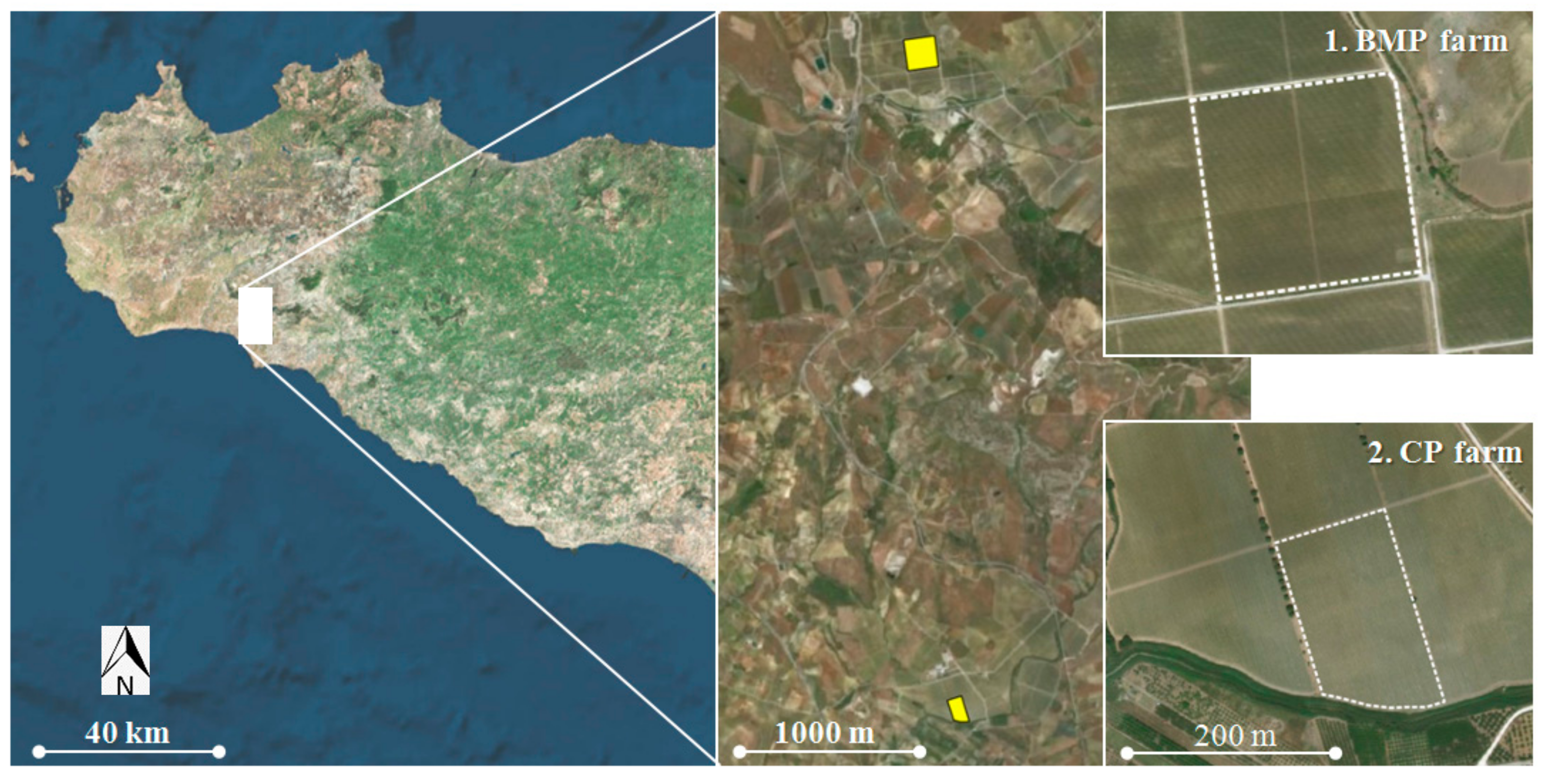
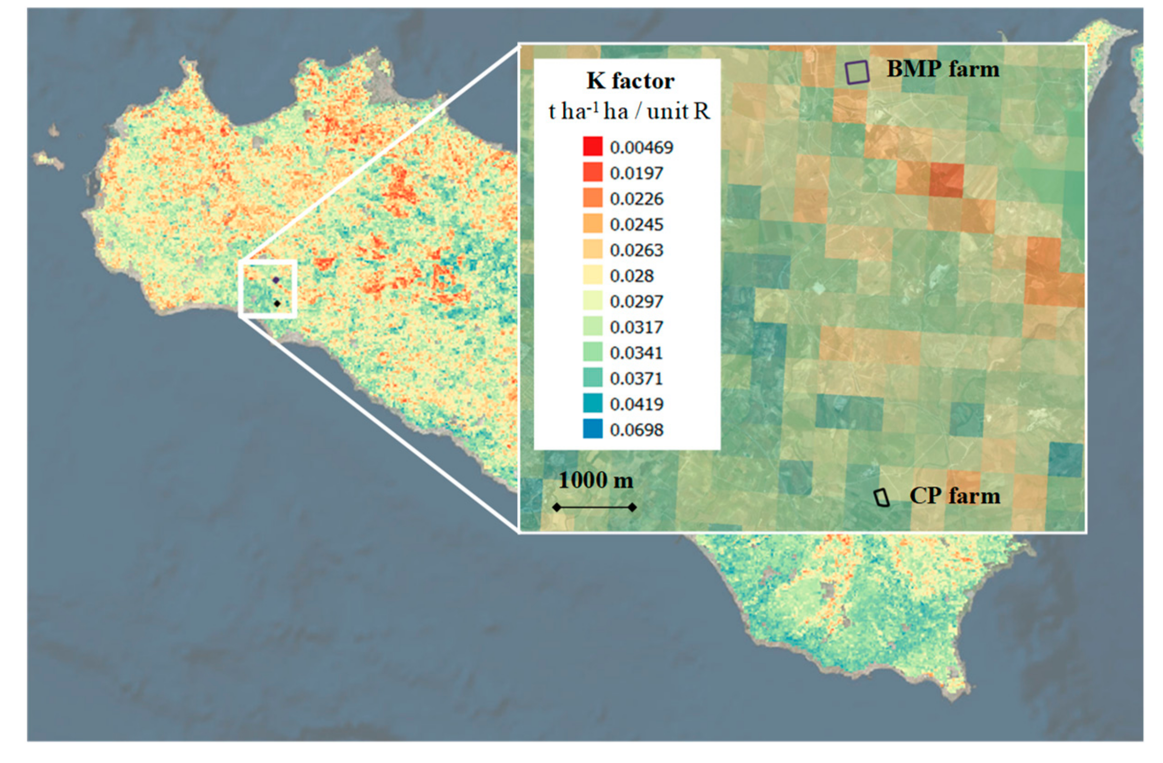
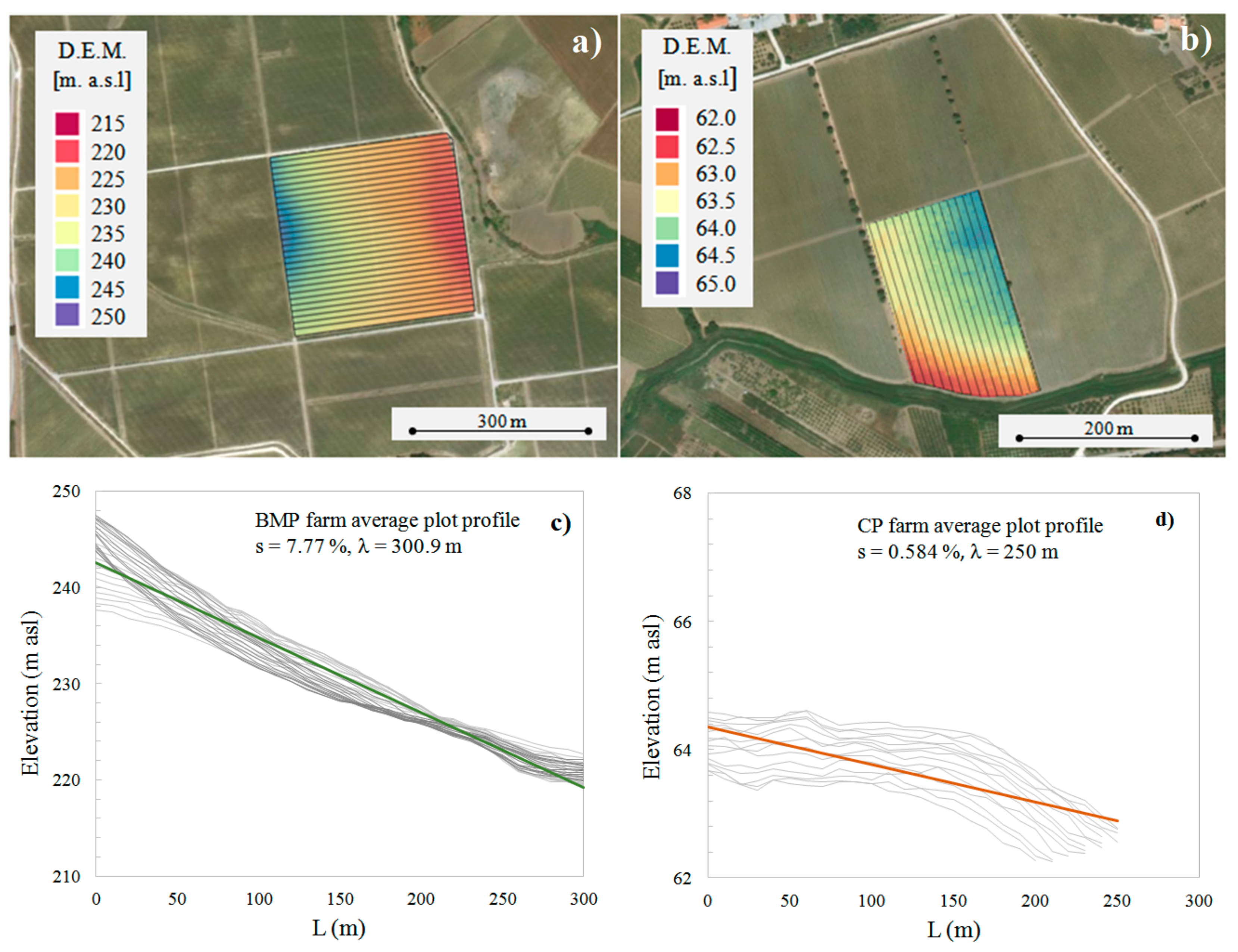
2.1. Study Area

The study area is located in southern Sicily (Figure 1) and is one of the 18 DOC (Controlled Denomination of Origin) vineyards areas on the island. For the studied area, the mean annual precipitation is 516 mm. On average, 3% of the mean annual rainfall occurs during summer (June, July, and August) while 42% occurs during November, December, and January. The minimum, maximum and mean of annual average incoming global solar radiation and vap pressure deficit (VPD) of the investigated areas are equal to 21, 353 and 223 W m⁻² and 0.03, 2.41 and 0.7 kPa, respectively. Two vineyards with different soil management were selected (Figure 1): One vineyard was managed with at least five shallow tillages per year (Conventional Practice farm—CP farm) to control weeds and reduce water competition, by using a field cultivator with a working width equal to 1.5 m and equipped with seven steel shanks; the other vineyard was managed (Best Management Practice—BMP farm) with agro-environmental measure management involving annual cover cropping using legumes like faba bean (Vicia faba) were investigated. In both surveyed areas, the soil was classified as Vertic Haploxerept according to Soil Taxonomy, with 58.3% and 51.2% sand, 11% and 13.5% silt, and 30.7% and 35.3% clay in the topsoil (0–20 cm) in BMP and CP farm, respectively.

The two vineyards were around 3.6 km from each other. The main features driving the choice of the two farms were (i) a sufficient uniform area matching the spatial resolution of MODIS data, (ii) BMP adoption under temporary cover crop during the winter period. The two farms are characterized by different slope and length (7.8% and 301 m for BMP and 0.6% and 250 m for CP farm).

2.2. The RUSLE Model

Following the original USLE model, the RUSLE computes the yearly soil loss erosion according to the equation:

𝐴 = 𝑅 × 𝐾 × 𝐿 × 𝑆 × 𝐶 × 𝑃

(1)

where A is the mean annual soil loss (t ha⁻¹ year⁻¹), R is the rainfall erosivity factor (MJ mm ha⁻¹ h⁻¹ year⁻¹), K is the soil erodibility factor (t ha h MJ⁻¹ h⁻¹ mm⁻¹), L and S are the slope-length and the slope-steepness factors (dimensionless), C is the cover and management factor (dimensionless) and P is the support practice factor (dimensionless).

With respect to the original USLE formulation, the revised USLE equation includes improvements in the sub-factors estimation, which were tested in a number of applications and experimental studies performed in many countries [12]. The detailed description of RUSLE factors algorithm is reported in the handbook edited by Renard et al. [1].

Recently, Panagos et al. [11] applied the RUSLE model for all of Europe providing a soil loss map with a detailed spatial resolution, although limited to an average annual soil loss estimation. However, uncertainties from soil erosion modeling arose from applications focused on intra-annual soil loss variability investigations that the RUSLE is also able to consider. In fact, although Equation (1) is usually applied for estimating yearly soil loss, by using the annual R-factor retrieved by iso-erodent maps or annual rainfall data [13,14], the RUSLE model can be also applied at a time scale shorter than the year, up until the event scale. In this case, sub-daily rainfall data is required in order to compute the single event rainfall erosivity index, R_e:

$$R_e=E{I}_{30}=\left({\displaystyle \sum }_{i=1}^k{e}_i^i{h}_i\right)I_{30}$$

(2)

where e_i is the unit rainfall energy (MJ ha⁻¹ mm⁻¹) and h_i the rainfall volume (mm) during the ith time period of a rainfall event divided in k-parts. I₃₀ is the maximum 30-minutes rainfall intensity (mm h⁻¹). The unit rainfall energy, e_i’, is calculated for each time interval as follows:

$$e_i^{\prime }=0.29\left[1-0.72exp\left(-0.05I_i\right)\right]$$

(3)

where I_i (mm h⁻¹) is the rainfall intensity during the time interval, h_i/t_i.

According to the RUSLE handbook [1], the erosive rainfall events were computed based on the following criteria: (i) The cumulative rainfall of an event is greater than 12.7 mm, (ii) the event has at least one peak that is greater than 6.35 mm during a period of 15 min (or 12.7 mm during a period of 30 min), and (iii) a rainfall accumulation of less than 1.27 mm during a period of six hours splits a longer storm period into two storms.

In our case, in the 2007–2016 period, rainfall events partition according to (iii) was first detected by calculating the sequence of waiting times, also denoted as dry spells [15], between two consecutive rainfall events recorded at 10 min time-scale by using a MATLAB code. The described procedure was applied to the rainfall data-series collected by a single station of the Agro-Meteorological Information Service of Sicily (SIAS) covering both vineyards (Figure 2). Figure 2, also reports the different NVDI time-series collected for the two farms, which were used to derive the cover management C factor.

The C factor accounts for the influence of vegetation upon the soil erosion process, ranging from 0 to 1, where higher values indicate no cover effects, whereas lower values mean a strong cover effect resulting in very limited soil erosion. According to the RUSLE model, a combination of sub-factors, such as impacts of previous management, canopy height, surface cover and roughness, etc., can be used to estimate the C factor [1]. This method requires extensive knowledge of the study area’s cover characteristics and maybe not be suitable without detailed monitoring of agricultural management. To address this, many authors suggested evaluating the C-factor through the Normalized Difference Vegetation Index (NDVI) obtained from satellite imagery [10,16,17,18]. This index has been widely used to map, at various observation scales, crop variables like biomass Leaf Area Index, LAI, plant coverage, etc. [19,20]. NDVI can be obtained from multispectral sensors able to capture reflectance images in red (RED) and infrared (NIR) spectral regions and was computed using the following expression:

$$\mathrm{NDVI}=\left(\frac{\mathrm{NIR}-\mathrm{RED}}{\mathrm{NIR}+\mathrm{RED}}\right)$$

(4)

An advantage of using NDVI consists of the capability to determine sub-annual C values, if satellite images are available, which can lead to understanding the cover contribute to seasonal soil erosion and to identify critical periods within the year where soil erosion could be considered a risk [4]. Following this approach, we used the global dataset of NDVI time-series at 8 and 16-day time-steps for the 2007–2016 period, provided by NASA using data from MODIS platforms (satellites Terra and Aqua), which can be retrieved from the Land Processes Distributed Active Archive Center [7]. The use of the MODIS NDVI time-series product was also supported considering its spatial resolution equal to 250 m which resulted appropriate for representing the two vineyard plots.

In order to transform the observed NDVI in a corresponding C factor, the following equation suggested and validated by Van der Knijff et al. [10], was applied:

$$C=exp\left(\frac{-2\mathrm{NDVI}}{1-\mathrm{NDVI}}\right)$$

(5)

Application of the RUSLE model also required the K factor estimation, which represents the influence of different soil properties on the slope’s susceptibility to erosion [1]. K factor also defines the “mean annual soil loss per unit of rainfall erosivity for a standard condition of bare soil, recently tilled up down slope with no conservation practice” [21]. In the RUSLE, Renard et al. [1] proposed an equation that relates textural and organic matter characteristics, soil structure and profile-permeability with the K factor or soil erodibility factor.

Recently, the new soil erodibility map for Europe generated by Panagos et al. [22] using the Land Use/Cover Area Frame Survey (LUCAS) soil European data-set, allowed a rough evaluation of the K factor in absence of the required soil textural information for the K factor RUSLE estimation. Following this approach, a value of 0.03 t ha⁻¹ ha h MJ⁻¹ mm⁻¹ was estimated for both considered vineyards (Figure 3).

As far as the LS factor, which accounts for the influence of the slope’s length and steepness of soil erosion processes, it is defined as the ratio of expected soil loss from a field slope relative to the original USLE unit plot [23]. The USLE method of calculating the slope length and steepness factor was originally applied at the unit plot and field scale, and the RUSLE extended this to the one-dimensional hillslope scale, with different equations depending on the slope gradient [1].

The LS factor was extended to topographically complex units using a method that incorporates contributing area and flow accumulation [24] derived from DEM and GIS approaches. In our case, a high-resolution DEM was used to assess LS factor of the two vineyard plots. However, the almost planar topography of the two plots suggested not using the contributing area and flow accumulation algorithms, restricting the use of DEM for an accurate estimation of the planar slope of the two plots (Figure 4).

Therefore, according to Renard et al. [1] the following L and S relationships were applied:

$$L={\left(\frac{\lambda }{22.1}\right)}^m$$

(6)

$$S=a sen\beta +b$$

(7)

where λ (m) is the plot length, β is the plot angle on the horizontal whereas the coefficients m, a, b, F, and p have the following expressions and values:

$$m=\left(\frac{pF}{1+pF}\right)$$

(8)

$$F=\left(\frac{sen\beta /0.0896}{3se{n}^{0.8}\beta +0.56}\right)$$

(9)

p = 0.5 − 2 (interrill − rill)

(10)

a = 10.8 (if tanβ < 0.09) or 16.8 (if tanβ ≥ 0.09)

(11)

b = 0.03 (if tanβ < 0.09) or −0.50 (if tanβ ≥ 0.09)

(12)

The P factor of Equation (1) accounts for management practices that affect soil erosion by modifying the flow pattern, such as contouring, strip-cropping, or terracing. The P factor is defined as the ratio between the soil loss under a specific soil conservation practice and that corresponding to a field with upslope and downslope tillage [1]. In our case, since no support practices were adopted in the two vineyard plots, the P factor was fixed equal to the unity [25].

3. Results and Discussion

Using the input data-set described in the previous section, the RUSLE model was applied at different time-scales of aggregations. The weekly data, which corresponds to the minimum C factor temporal scale of observation, were aggregated in annual, seasonal, monthly and the RUSLE input factors were accordingly analyzed.

With the aim to evaluate the C and R factor interactions, disaggregated data in the two vineyards were analyzed. In this case, in order to evaluate soil erosion independently from the highly different topographic characteristics of the two plots, the product of R, K and C factor, RKC, which refers to soil loss (t ha⁻¹) per LS unit, was also investigated.

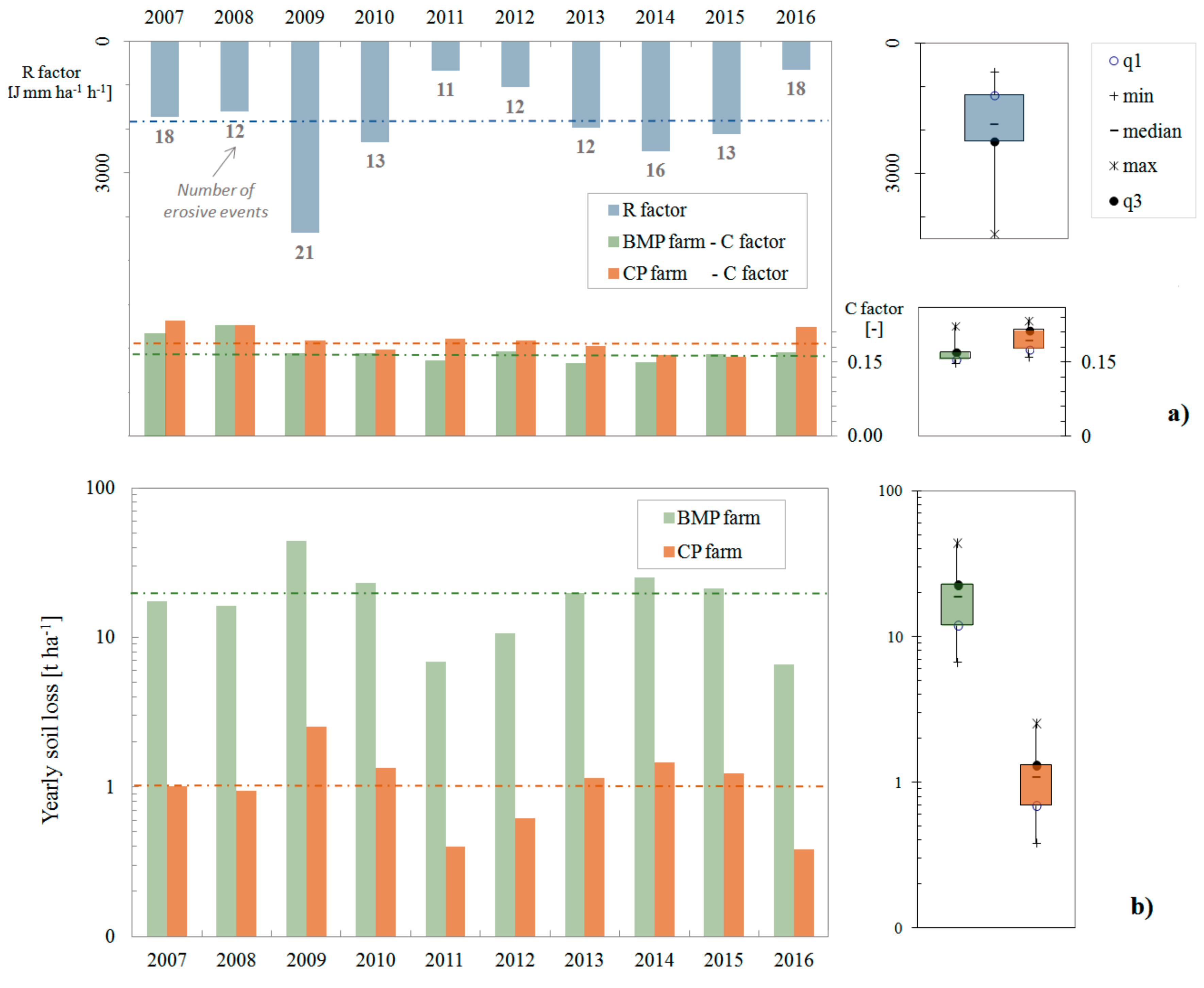
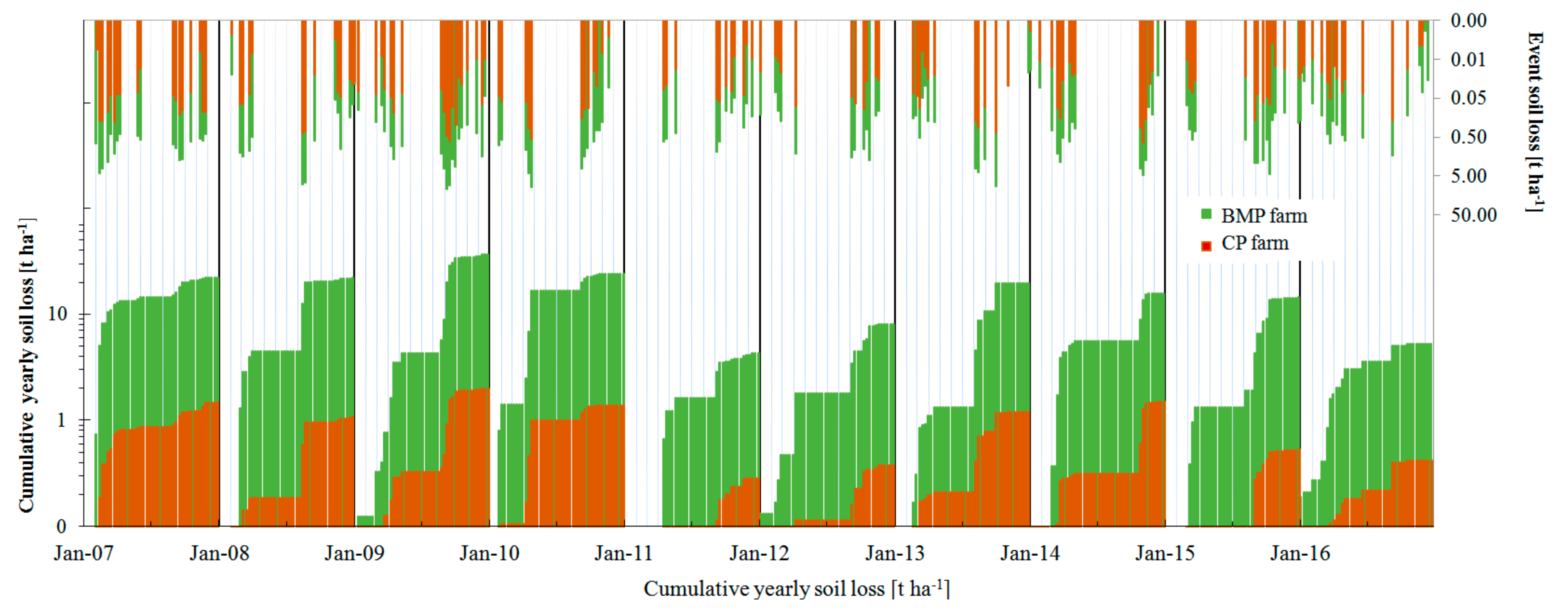
3.1. Yearly and Monthly Average Soil Loss

The ten-year calculated R factor (Figure 5a) shows a high interannual variability ranging from 661–4377 MJ mm ha⁻¹ h⁻¹. The R factor variability appears not correlated to the number of erosive events, N_ev, (Figure 5a), whereas it seems dependent on the annual rainfall, H_y (Figure 2).

As an example, the yearly R factor value in 2015 (R = 2122 t ha MJ mm ha⁻¹ h⁻¹, H_y = 705 mm, N_ev = 13) resulted much higher than 2016 (R = 661 t ha MJ mm ha⁻¹ h⁻¹, h_an = 505 mm, N_ev = 18), evidencing for the latter case the occurrence of lower energy rainfall values than the former one.

Differences between the two vineyards characterized by different soil management, in terms of yearly C values, appear almost slight with a greater variability for CP farm than BMP farm (Figure 5a), although differences in terms of ten-year average C values are appreciable (see dash-dot lines). The higher variability of the C factor for CP than BMP farm can be ascribed to the unpredictable rainfall regime that affects the time scheduling of soil practices (see box plots Figure 5a).

The yearly soil loss calculated by the RUSLE model (Figure 5b) mainly reflects the variability of the R factor, as a consequence of the slight aforementioned C factor variability and of the lumped K and LS factors assumed for the two vineyards. Generally, yearly soil loss between the two vineyards are characterized by the same interannual variability (see box plot, Figure 5b). The large differences in yearly soil loss between the two vineyards are mainly due to the different LS factors (LS = 1.9, for BMP farm and LS = 0.1 for the CP farm). Results illustrated in Figure 5b highlight the prevailing role played by the R factor rather than the C factor in determining soil erosion when input data at a higher temporal scale are analyzed, and suggested that inter-annual and intra-annual soil erosion variability needs considering.

Event scale input data and the corresponding results of the RUSLE model in the two vineyard farms are reported in Figure 6 and Figure 7, respectively.

Figure 6 indicates that generally high values of R factors occur when the two plots are characterized by low C values, suggesting the need of cover crop soil management in the corresponding periods. Analysis at the event scale allows detecting R and C factor interactions evidencing the occurrence of peak R factor that could also be associated with high differences in C values between BMP and CP farms. See, as an example, the difference in the peaks of R values in 2013 and 2014 and the corresponding C factors (Figure 6) that on a yearly scale was not possible to detect. In particular, the greater peak of the R value in 2014 rather than in 2013 is associated with higher differences in C values.

The cumulative yearly soil loss generally shows a drop occurring in the second semester of the year (Figure 7), which corresponds to high R values that in turn are affected by high rainfall intensities, concentrated after the summer season, typical of the Mediterranean region [26]. These results suggest that the analysis at the event scale could help in identifying the most critical period for erosion risks and the importance of alternative soil management, including BMP or spontaneous vegetation cover. Differences in cumulative yearly soil loss between the two plots of around one order of magnitude are of course due to the LS factor, making it difficult to discuss the effect of the cover crop factor alone and its interactions with the R factor in terms of soil loss.

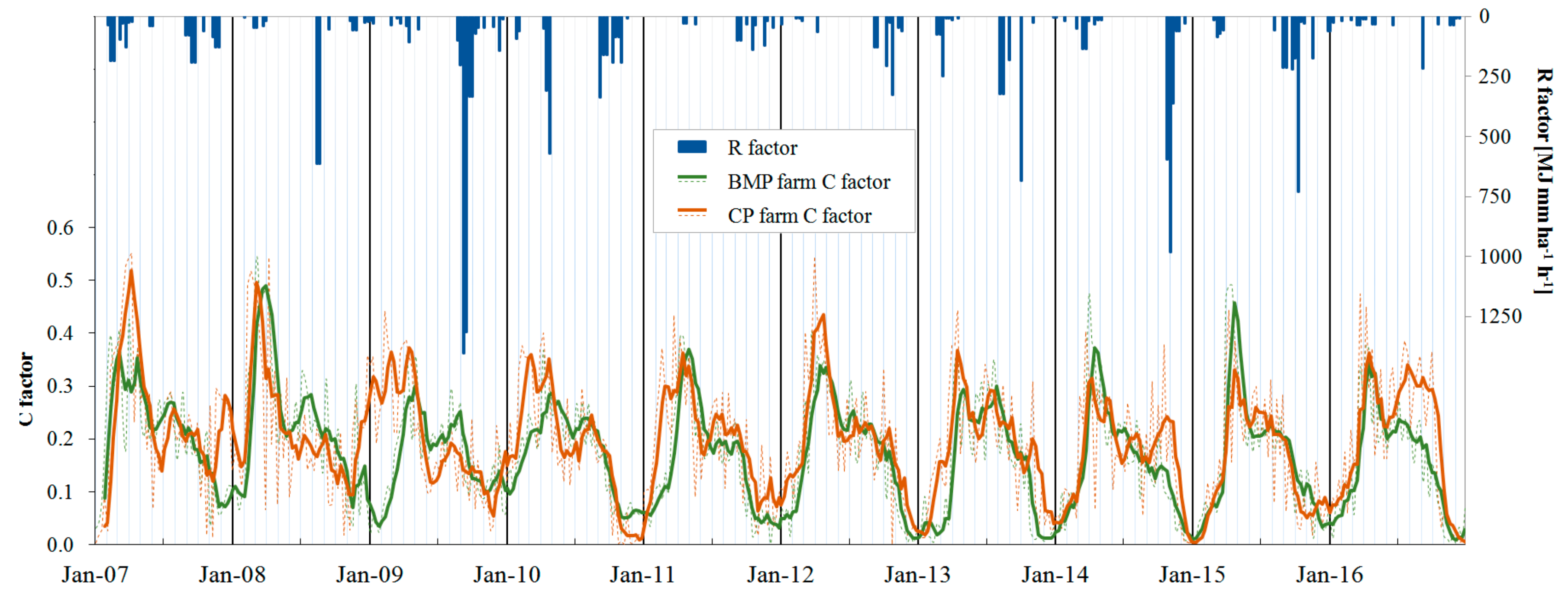
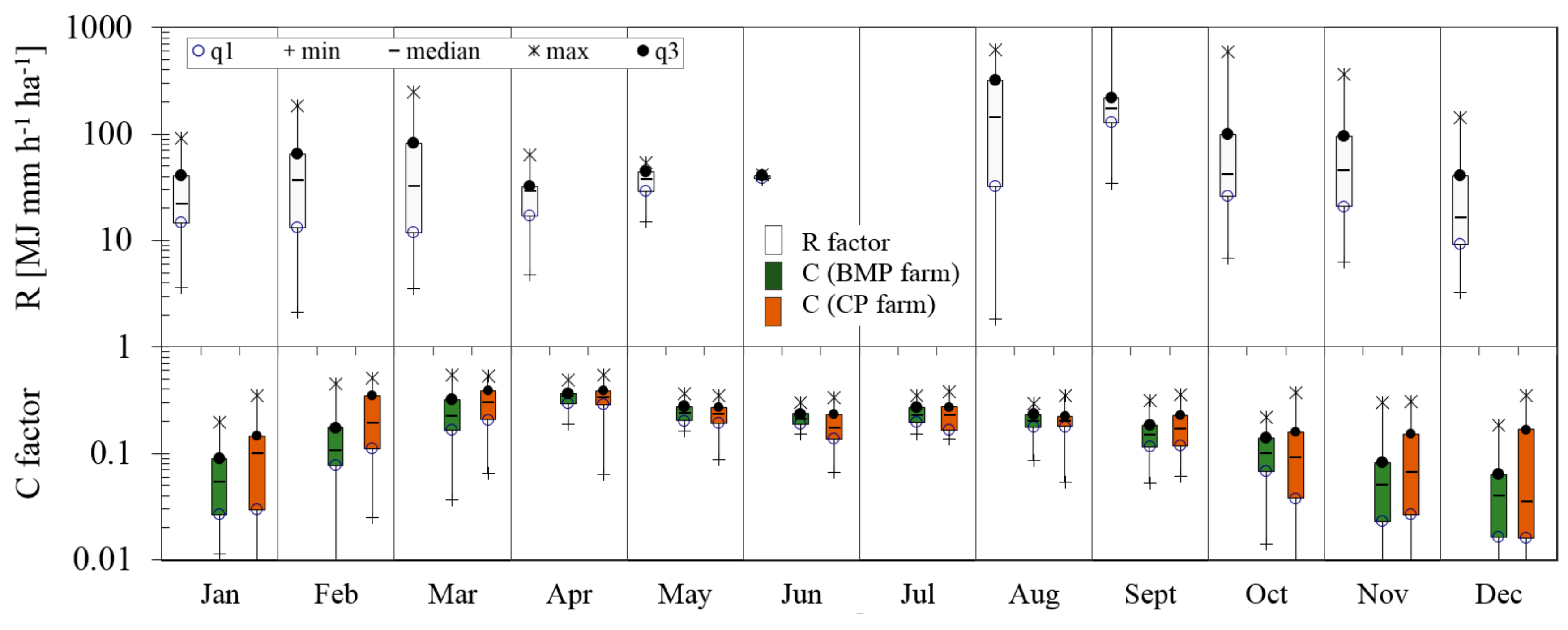
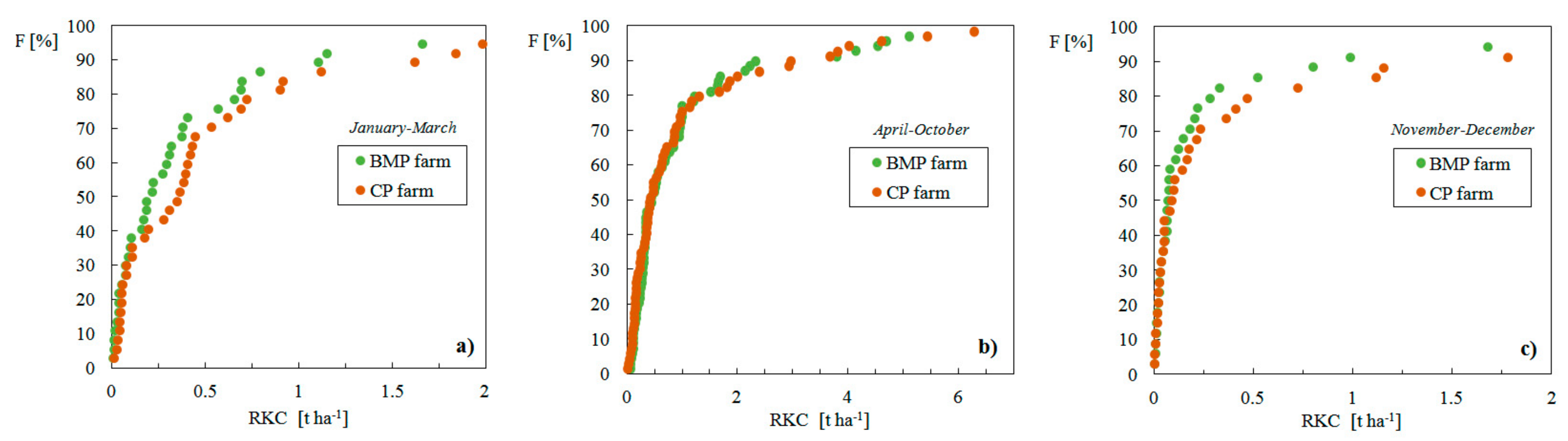
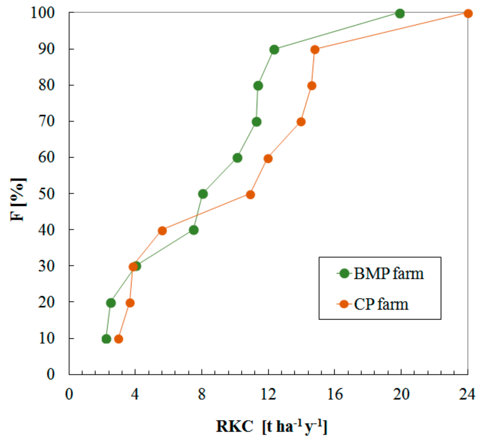
3.2. C and R Factors Seasonal Interactions and Impact of Crop Management

Results described in Section 3.1 suggest exploring the C and R factors intra-annual interactions, which rather than a simple analysis of means (Figure 5), allow emphasizing the impact of soil management practice and at the same time, the extremes and intra-annual dynamics.

From summer to autumn, seasonal R factor increases, with the median peak (R = 173 MJ mm h⁻¹ ha⁻¹) in September (Figure 8). High R factor values also occurred in the winter season with the median value (R = 37 MJ mm h⁻¹ ha⁻¹) in February. During these periods, different C factor distributions between the considered plots could be observed. In particular, C factor values corresponding to BMP farm generally resulted lower than the CP farm, as a consequence of the different cover cropping management. On the contrary, during the April–October period, a C factor invariance between BMP and CP management due to the dominant vigor of vineyard canopy was observed.

Differences in the C factor between the two plots, and its interactions with the R factor, can be better evidenced if referring to soil loss per unit of the LS factor. Moreover, in order to assess the importance of seasonal C and R factors and their temporal interactions, compared to the corresponding annual values, for the periods January–March, April–October and November–December, in Figure 9 frequency distributions of soil loss per unit LS are plotted. For the January–March period (Figure 9a), the lower RKC values of the BMP farm provide lower soil loss values than the CP farm and a similar behavior occurs during the November–December period (Figure 9c), especially for high frequencies. Contrarily, during the April–October period (Figure 9b), no significant differences between the two vineyards can be observed. This result could be ascribed to the temporary cover crop and to conventional soil management, which characterizes BMP and CP farms, respectively.

Figure 10 shows the distributions of yearly soil loss per unit LS and P (RKC) for BMP and CP farms. At low frequencies there is no relevant effect of management practice, whereas for high frequencies the corresponding RKC value is generally lower for the BMP than the CP farm, indicating the positive impact of BMP cover management independently from the slope of the two plots. These results indicate that despite the seasonal R and C factors interactions and the differences between the two farms could not appear relevant, it seems they play an important role at the annual scale.

Finally, in order to assess the effectiveness of cover crop management in controlling soil loss, yearly soil loss assuming a different scenario of management practice consisting of no cover cropping was assumed. In particular, C values corresponding to CP management were applied to the BMP farm. This choice was justified by considering that the observed BMP and CP C factors are almost invariant during the period covering phenological vineyard cycle (April–October, see Figure 9), while they vary during the remaining periods according to the different management practice.

In Figure 11, the difference between soil loss calculated for the actual BMP farm and those calculated with the different management practice mentioned above denoted as saved soil loss is plotted for the ten-year investigated period.

The same figure illustrates the cumulative saved soil loss. Results show that, usually, cover cropping management produced an important reduction of soil loss rate with respect to CP management with a total saved soil loss around 32 t ha⁻¹ during the observed period (2007–2016) (Figure 11). The average saved soil loss over the 10-year period was equal to 3.2 t ha⁻¹ with a maximum of 13.2 t ha⁻¹ in 2014 (Figure 11). Interesting, the latter result reflects the seasonal R and C factor interactions discussed in Figure 6.

4. Conclusions

In the Mediterranean environment, hilly vineyards have higher soil losses compared to other rainfed cropping systems (cereals, olives) [27]. High erosion rates are mainly due to (i) bare soil conditions for most of the year and (ii) the vine rows orientation along highest slopes, which favor water runoff and sediment yields.

Several authors describe the effectiveness of Best Management Practice (BMP) as an important tool to prevent soil erosion rather than Conventional Practice (CP), but at the same time, they stress on the high soil loss variability due to the interaction of several factors characterized by large uncertainty [28,29].

In the near future, rainfall intensity will increase in mid-latitude areas [30,31]. One of the effects of higher rainfall intensity is increasing soil erosion, suggesting that cover crop management (BMP) can be used as an adaptation tool to this type of climate change [28].

This paper shows the importance of appropriate R and C factor assessment and their inter- and intra-annual interactions in determining soil erosion variability, by using climatic input data at a high temporal scale resolution for the R factor, and remotely sensed NDVI time-series for the C factor. It is known that the variability of C factor is managed by human activity and it is less subjected to the unpredictability of natural events as is the R factor. Indeed, the C factor is also subjected to uncertainty in relation to weather and to all related agronomic practices (species choice, seeding date, emergence, crop development, etc.). Moreover, the use of control measures (BMP) requires prudent knowledge of land management at the farm level [32] and a deep awareness of the driving forces determining soil erosion.

In this paper, starting from temporally detailed data-set, the RUSLE model was applied at different time-scales of aggregations for two different managed vineyards (BMP and CP farms). In particular, RUSLE application at yearly, seasonal, monthly and event scales of aggregation was performed. Results showed that at a yearly scale the soil loss mainly reflects the variability of the annual R factor, as a consequence of the slight annual C factor variability for the two selected vineyards, which appeared almost greater for the CP farm than the BMP farm. Moreover, at a yearly scale no interaction between R and C factors arose.

Differences in the C factor between the two plots, and their interactions with the R factor, were better evidenced at seasonal, monthly and event scale if referring to soil loss per unit LS and P factors, RKC. In particular, for the January–March period, the lower RKC values of the BMP farm provide lower soil loss values than the CP farm and a similar behaviour occurs in the November–December period. At these scales, high values of R factors generally occurred when the two plots were characterized by low C values, suggesting the need for cover crop soil management in the corresponding periods. Furthermore, the impact of BMP in preventing soil erosion was described in terms of average saved soil loss, which over the 10-year period of observation was equal to 3.2 t ha⁻¹ with a maximum of 13.2 t ha⁻¹ in 2014.

The evaluation of soil erosion at a different temporal scale and its implications can help stakeholders and scientists formulate better soil conservation practices and agricultural management, also considering that erosivity rates are expected to increase to account for the increase of rainfall intensity.

Finally, the introduction of a nature-based solution (large use of spontaneous cover cropping, permanent cover cropping, etc.), could be the new paradigm of soil conservation management, especially in semi-arid vineyards. All those management strategies increase resilience and reduce vineyard system vulnerability, representing a concrete adaptation strategy.

References

1. Renard, K.G.; Foster, G.R.; Weesies, G.A.; McCool, D.K.; Yoder, D.C. Predicting Soil Erosion by Water: A Guide to Conservation Planning with the Revised Universal Soil Loss Equation (RUSLE); Agriculture Handbook Number 703; US Government Printing Office: Washington, DC, USA, 1997.
2. De Santos Loureiro, N.; de Azevedo Coutinho, M. A new procedure to estimate the RUSLE EI30 Index, based on monthly rainfall data and applied to the Algarve region, Portugal. J. Hydrol. 2001, 250, 12–18. [Google Scholar] [CrossRef]
3. Nunes, A.N.; Lourenço, L.; Vieira, A.; Bento-Gonçalves, A. Precipitation and erosivity in Southern Portugal: Seasonal variability and trends (1950–2008). Land Degrad. Dev. 2016, 27, 211–222. [Google Scholar] [CrossRef]
4. Ferreira, V.; Panagopoulos, T. Seasonality of soil erosion under Mediterranean conditions at the Alqueva Dam watershed. Environ. Manag. 2014, 54, 67–83. [Google Scholar] [CrossRef]
5. Terranova, O.G.; Gariano, S.L. Rainstorms able to induce flash floods in a Mediterranean-climate region (Calabria, southern Italy). Nat. Hazards Earth Syst. Sci. 2014, 14, 2423–2434. [Google Scholar] [CrossRef]
6. D’Asaro, F.; D’Agostino, L.; Bagarello, V. Assessing changes in rainfall erosivity in Sicily during the twentieth century. Hydrol. Process. 2007, 21, 2862–2871. [Google Scholar] [CrossRef]
7. Land Processes Distributed Active Archive Center (LP DAAC). 1990. Available online: http://lpdaac.usgs.gov/ (accessed on 8 May 2019).
8. Karaburun, A.; Bhandari, A.K. Estimation of C factor for soil erosion modelling using NDVI in Buyukcekmece watershed. Ozean J. Appl. Sci. 2010, 3, 77–85. [Google Scholar]
9. Vicente, M.L.; Navas, A.; Machin, J. Identifying erosive periods by using RUSLE factors in mountain fields of the Central Spanish Pyrenees. Hydrol. Earth Syst. Sci. Discuss. 2007, 4, 2111–2142. [Google Scholar] [CrossRef]
10. Van der Knijff, J.M.; Jones, R.J.A.; Montanarella, L. Soil Erosion Risk Assessment in Europe; EUR 19044 EN; European Commission: Brussels, Belgium, 2000. [Google Scholar]
11. Panagos, P.; Borrelli, P.; Poesen, J.; Ballabio, C.; Lugato, E.; Meusburger, K.; Montanarella, L.; Alewell, C. The new assessment of soil loss by water erosion in Europe, Environ. Sci. Policy 2015, 54, 438–447. [Google Scholar] [CrossRef]
12. Benavidez, R.; Jackson, B.; Maxwell, D.; Norton, K. A review of the (Revised) Universal Soil Loss Equation ((R)USLE): With a view to increasing its global applicability and improving soil loss estimates. Hydrol. Earth Syst. Sci. 2018, 22, 6059–6086. [Google Scholar] [CrossRef]
13. Ferro, V.; Giordano, G.; Iovino, M. Isoerosivity and erosion risk map for Sicily. Hydrol. Sci. J. 1991, 36, 549–564. [Google Scholar] [CrossRef]
14. Ballabio, C.; Borrelli, P.; Spinoni, J.; Meusburger, K.; Michaelides, S.; Beguería, S.; Klik, A.; Petan, S.; Janeček, M.; Olsen, P.; et al. Mapping monthly rainfall erosivity in Europe. Sci. Total Environ. 2017, 579, 1298–1315. [Google Scholar] [CrossRef] [PubMed]
15. Baiamonte, G.; Mercalli, L.; Cat Berro, D.; Agnese, C.; Ferraris, S. Modelling the frequency distribution of interarrival times from daily precipitation time-series in North-West Italy. Hydrol. Res. 2018, 50, 339–357. [Google Scholar] [CrossRef]
16. Ma, B.L.; Dwyer, L.M.; Costa, C.; Cober, E.R.; Morrison, M.J. Early prediction of soybean yield from canopy reflectance measurements. Agron. J. 2001, 93, 1227–1234. [Google Scholar] [CrossRef]
17. De Asis, A.M.; Omasa, K. Estimation of vegetation parameter for modeling soil erosion using linear Spectral Mixture Analysis of Landsat ETM data. ISPRS J. Photogramm. Remote. Sens. 2007, 62, 309–324. [Google Scholar] [CrossRef]
18. Li, C.; Qi, J.; Yang, L.; Wang, S.; Yang, W.; Zhu, G.; Zou, S.; Zhang, F. Regional vegetation dynamics and its response to climate change—A case study in the Tao River Basin in Northwestern China. Environ. Res. Lett. 2014, 9, 12500. [Google Scholar] [CrossRef]
19. Christensen, S.; Goudriaan, J. Deriving light interception and biomass from spectral reflectance ratio. Remote Sens. Environ. 1993, 43, 87–95. [Google Scholar] [CrossRef]
20. Aparicio, N.; Villegas, D.; Casadesus, J.; Araus, J.L.; Royo, C. Spectral vegetation indices as nondestructive tools for determining durum wheat yield. Agron. J. 2000, 92, 83–91. [Google Scholar] [CrossRef]
21. Morgan, R.P.C. Soil Erosion and Conservation. In Environmental Modelling: Finding Simplicity in Complexity, 2nd ed.; Blackwell Publishing: Oxford, UK, 2005. [Google Scholar]
22. Panagos, P.; Meusburger, K.; Ballabio, C.; Borrelli, P.; Alewell, C. Soil erodibility in Europe: A high-resolution dataset based on LUCAS. Sci. Total Environ. 2014, 479, 189–200. [Google Scholar] [CrossRef]
23. Wischmeier, W.H.; Smith, D.D. Predicting Rainfall Erosion Losses: Guide to Conservation Planning USDA; Agriculture Handbook Number 537; U.S. Government Printing Office: Washington, DC, USA, 1978.
24. Desmet, P.J.; Govers, G. A GIS procedure for automatically calculating the USLE LS factor on topographically complex landscape units. J. Soil Water Conserv. 1996, 51, 427–433. [Google Scholar]
25. Adornado, H.A.; Yoshida, M.; Apolinares, H.A. Erosion vulnerability assessment in REINA, Quezon Province, Philippines with raster-based tool built within GIS environment. Agric. Inf. Res. 2009, 18, 24–31. [Google Scholar] [CrossRef]
26. Agnese, C.; Baiamonte, G.; Cammalleri, C. Modelling the occurrence of rainy days under a typical Mediterranean climate. Adv. Water Res. 2014, 64, 62–76. [Google Scholar] [CrossRef]
27. Kosmas, C.; Danalatos, N.; Cammeraat, L.H.; Chabart, M.; Diamantopoulos, J.; Farand, R.; Gutierreze, L.; Jacob, A.; Marques, H.; Martinez-Fernandezg, J.; et al. The effect of land use on runoff and soil erosion rates under Mediterranean conditions. Catena 1997, 29, 45–59. [Google Scholar] [CrossRef]
28. Novara, A.; Gristina, L.; Saladino, S.S.; Santoro, A.; Cerdà, A. Soil erosion assessment on tillage and alternative soil managements in a Sicilian vineyard. Soil Tillage Res. 2011, 117. [Google Scholar] [CrossRef]
29. Baiamonte, G.; D’Asaro, F. Discussion of “Analysis of extreme rainfall trends in sicily for the evaluation of depth-duration-frequency curves in climate change scenarios, by Lorena Liuzzo and Gabriele Freni”. J. Hydrol. E ASCE 2016, 21. [Google Scholar] [CrossRef]
30. IPCC. Climate Change 2013: The Physical Science Basis. Contribution of Working Group I to the Fifth Assessment Report of the Intergovernmental Panel on Climate Change; Stock, T.F., Qin, D., Plattner, G.-K., Tignor, M., Allen, S.K., Boschung, J., Nauels, A., Xia, Y., Bex, V., Midgley, P.M., Eds.; Cambridge University Press: Cambridge, UK, 2013. [Google Scholar]
31. Trenberth, K.E. Changes in precipitation with climate change. Clim. Res. 2011, 47, 123–138. [Google Scholar] [CrossRef]
32. Kessler, A.; De Graaff, J.; Olsen, P. Farm-level adoption of soil and water conservation measures and policy implications in Europe. Land Use Policy 2010, 27, 1–3. [Google Scholar] [CrossRef]
Figure 1. Geographic location of the study area in the Sicily region. The two different investigated vineyards (Best Management Practices, BMP, and Conventional Practice farm, CP, farms) are illustrated.
Water 11 00978 g001
Figure 2. Rainfall data and Modis NDVI time-series used in the investigation.
Water 11 00978 g002
Figure 3. Spatial variability of soil erodibility K factor over the study area [22].
Water 11 00978 g003
Figure 4. Elevation and topographic attributes of the two vineyards plots. (a) BMP farm, (b) CP farm, (c) BMP farm average profile, (d) CP farm average profile.
Water 11 00978 g004
Figure 5. (a) Rainfall erosivity (R) and cover management (C) factors and (b) output results of the RUSLE model applied at average yearly and annual time scale. In the right of both figures the box-plots of the corresponding variables are also reported (q1 and q3 are the first and the third quartiles).
Water 11 00978 g005
Figure 6. R and C factors calculated at event time-scale for the two vineyard plots during the investigated period.
Water 11 00978 g006
Figure 7. Event and cumulative yearly soil loss estimated using RUSLE model for the two vineyard plots during the investigated period.
Water 11 00978 g007
Figure 8. Box-plots of the monthly variability of R and C factors for the two investigated plots (q1 and q3 are the first and the third quartiles).
Water 11 00978 g008
Figure 9. Seasonal distributions of soil loss per unit LS and P, RKC (see RUSLE model), for the two investigated plots. F is the frequency of non-exceedance. (a) January–March period, (b) April–October period, (c) November–December period.
Water 11 00978 g009
Figure 10. Distributions of yearly soil loss per unit LS and P, RKC (see RUSLE model), for the two investigated vineyards. F is the frequency of non-exceedance.
Water 11 00978 g010
Figure 11. Impact of BMP scenario on saved soil loss. Solid line is the cumulative saved soil loss, whereas the histogram and the corresponding box-plot refer to the annual saved soil loss (q1 and q3 are the first and the third quartiles).
Water 11 00978 g011