A Modeling Approach to Diagnose the Impacts of Global Changes on Discharge and Suspended Sediment Concentration within the Red River Basin

Abstract

The Red River basin is a typical Asian river system affected by climate and anthropogenic changes. The purpose of this study is to build a tool to separate the effect of climate variability and anthropogenic influences on hydrology and suspended sediments. A modeling method combining in situ and climatic satellite data was used to analyze the discharge (Q) and suspended sediment concentration (SSC) at a daily time scale from 2000 to 2014. Scenarios of natural and actual conditions were implemented to quantify the impacts of climate variability and dams. The modeling gained satisfactory simulation results of water regime and SSC compared to the observations. Under natural conditions, the Q and SSC show decreasing tendencies, and climate variability is the main influence factor reducing the Q. Under actual conditions, SSC is mainly reduced by dams. At the outlet, annual mean Q got reduced by 13% (9% by climate and 4% by dams), and annual mean SSC got reduced to 89% (13% due to climate and 76% due to dams) of that under natural conditions. The climate tendencies are mainly explained by a decrease of 9% on precipitation and 5% on evapotranspiration, which results in a 13% decrease of available water for the whole basin.

1. Introduction

Nowadays, the freshwater scarcity has become a global and local dramatic threat for the sustainable development of the human society [1]. The continuous increasing water demand is growing faster than the demographic increase, bringing the water crises as a major world risk [2]. River network plays a critical role in hydrological cycle, and also in processing and transporting sediments and nutrients to oceans. The suspended sediment (SS) transportation by rivers can be a reflection of land and river degradation, and it drives nutrients to the seas which is an essential process for marine biogeochemical cycle and diversity [3,4].

Hydrological cycle and water quality are affected by climate variability and human disturbance. Climate variations, particularly temperature and precipitation, have effects on river systems both at short and long time scales, such as floods and droughts caused by typhoons and El Nino and La Nina, especially in the tropics [5,6,7]. In addition, under the disturbance of human activities (such as industrial and agricultural water consumption and dam constructions), water ecosystems are facing severe challenge, like the increase of soil erosion, pollutants and nutrient loads, and changes of hydrology regime and sediment fluxes (SF) [8,9,10,11,12,13].

To face the challenge of increasing water demand under uncertain variations of climate, dams have been built globally for water storage. Globally, at least 45,000 large dams have been built, and nearly half of the world’s rivers have at least one large dam [14]. From a Global Reservoir and Dam database, approximate 28% dams are located in Asia [15]. In addition, future hydropower development is primarily concentrated in developing countries and emerging economies of Southeast Asia [16]. As a consequence, dams coupled to climate variability have an impact on water regime and fluxes of matters, mainly SS [17]. Dam implementation can cause a significant reduction of SF; Vörösmarty et al. (2003) [18] estimated greater than 50% of potential sediment trapping by dams in regulated basins. However, reduced sediment transport affects estuarine and coastal communities [19]. For example, as a result of reduced sediment delivery, many river deltas are sinking, thereby increasing the vulnerability of human populations depending on their ecosystem services for survival [15].

Therefore, understanding and quantifying hydrology, soil and biogeochemical processes, and budgets are essential in managing water resource, in controlling and mitigating soil and pollutant loads. For achieving this, appropriate methods and tools are necessary, such as in-site field measurements, empirical and simple equations, remote sensing techniques, geographic information systems, and numerical simulations. However, field-collecting data at large spatial and temporal scales is expensive, and often impracticable in some remote areas and underdeveloped regions. Empirical or/and simple equations, such as sediment rating curves are sometimes applied to quantify the SF [20,21,22,23]. However, a sediment rating curve requires discharge (Q) as an input, which might not be available for remote and underdeveloped regions, and its parameters can vary a lot among a big drainage basin. Therefore, this method might neither be the best choice for calculating the SF at a daily basis nor in a large basin. Modeling is a good tool, combined with other techniques (such as remote sensing), to compensate the above shortages. Simulations can be carried out at a large spatial scale and at a daily time scale to quantify, analyze and forecast water resources and quality. In particular, it can realistically represent the spatial variability of the basin, which will provide a global view of the whole basin. Many physically based hydrological models had been used [24,25,26,27], such as MIKESHE [28], HSPF [29] and Soil and Water Assessment Tool (SWAT) [30]. Among these models, SWAT has been proved to obtain good hydrological predictions with a little direct calibration in many different basins around the world [26,27,31], and more applications can be found in SWAT literature database: https://www.card.iastate.edu/swat_articles/.

Although SWAT has been applied to many Asian basins, and also to subtropical or/and tropical areas, most of them were at a scale of 77 to 105,000 km² [31,32,33,34,35]. The Red River is a typical Asian river system, combining different land uses, affected by human activities such as intensive dam implementations and agriculture [36,37]. Recent studies of hydrology and suspended sediment in this basin mainly used data from gauge stations or sampling to do statistical analysis [38,39,40,41], or use modeling to perform simulations at a local scale [42] or in the delta part [43] at a monthly scale; few studies analyzed fluxes at daily scale, but only on a short period [37], in the delta [44] or only for discharge or suspended sediment [45]. Both Q and SSC can vary greatly from day to day; therefore, it would be more favourable to calculate flux at a daily scale. Also, water quality monitoring is usually carried out during some specific days in a month, and outputs from a model at daily scale can be practical and useful for further studies. In addition, different scenarios of global changes can be considered to help researchers or government administrators to compare different possibilities and set up long-term management plans.

Hence, the objective of this paper is to apply a new tool in the Red River basin to analyze hydrology and suspended sediment transport in order to diagnose impacts of the global changes by separating the effect of climate variability and anthropogenic influences. The model was applied: (1) to characterize the hydrology of the basin at daily scale; (2) to quantify the SSC in time and space; (3) to assess the impacts of climate variability and dams in a separate way.

2. Materials and Methods

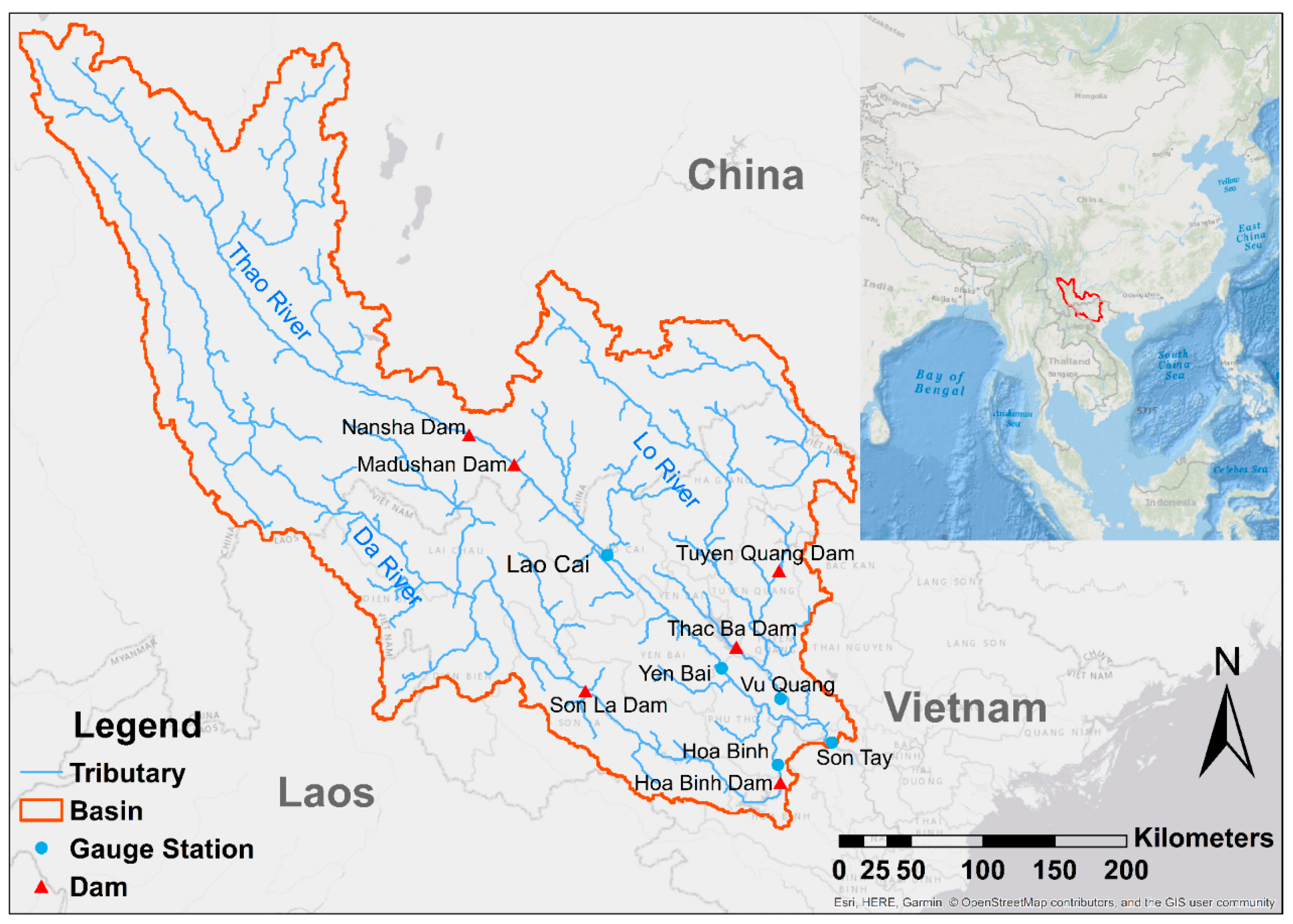
2.1. Study Area

2.1.1. General Characteristics

The Red River basin, located in the southeastern Asia, is a portion of the international border among China, Laos and Vietnam. Of the total area, 49% lies in China, 0.9% in Laos and 50.1% in Vietnam. The Red River originates in Dali, Yunnan Province (China), which is a mountainous region, at an elevation of 2650 m a.s.l. [46]. Due to the accessibility of the data and considering the influence of the tide, our study area focused only on the continental basin with a surface of 137,200 km² that drained down to Son Tay, which is the outlet of the continental basin and the entrance of the delta (Figure 1).

The upper part of the main river, before Son Tay, is called the Thao River. It receives two main tributaries: the Da River from the right bank, and the Lo River from the left bank. These two tributaries join the Red River just 20 km upstream to the Son Tay gauging station.

Rapid increase of population and intensive agriculture activities inside the Red River basin require more water supplies for urban, industry and agriculture use, and more and more dams and irrigation channels are built to meet these demands both in China and Vietnam. In the upstream of the Thao River in China, twelve cascade hydropower stations are under construction. The Nansha Dam and the Madushan Dam started impoundment on November 2007 and December 2010, respectively, on the Thao River. On the Da River, the biggest dam named Hoa Binh was put into use in 1989. The Hoa Binh dam has trapped a mass of solid materials, and sedimentation in the reservoir reduces the dam’s efficient capacity and life [39]. Therefore, in order to mitigate the siltation of the Hoa Binh dam and to meet the need of economic growth, the Son La dam (upstream) was built and put into use on December 2010. On the Lo River, the Thac Ba dam was implemented in 1972 and the Tuyen Quang dam was carried out on March 2008. More details of these dams can be found in

Table 1. Basic Characteristics of the Dams [41].

Name (Basin)	Construction	Operation	Capacity (× 109 m3)	Mean Water Level (m)	Mean Annual Discharge (m3/s)	Maximum Discharge (m3/s)
Nansha (Thao)	February 2006	November 2007	0.26	267	261	–
Madushan (Thao)	December 2008	December 2010	0.55	217	302	–
Hoa Binh (Da)	1980	1989	9.50	115	1780	2400
Son La (Da)	December 2005	December 2010	9.26	215	1530	3438
Thac Ba (Lo)	1965	October 1971	2.90	58	190	420
Tuyen Quang (Lo)	December 2002	March 2008	2.24	120	318	750

.

The upstream part in China is dominated by tectonically active montane areas with steep slopes, usually above 25° [47]. Intensive rainfall and prominent contradiction between human and land make this area vulnerable to high erosion with steep slopes [38,48,49]. The main soil types are Acrisols, such as latosol, red earth, yellow brown soil and fluvisol [48,50]. Therefore, high erosion plus the character of soil types colour the water of the Thao River and the Da River into “red” [50]. In Vietnam, the same Acrisols dominate on the slopes, and grey or alluvial soils dominate in the valleys [41]. Land use in China is mainly forest, accounting for 62% of the area, followed by grassland and cultivated land, accounting for 19% and 18%, respectively [1] (Li et al., 2016). Land use varies in Vietnam in different sub-basins: in the main stream basin (Thao basin), forest is the dominant land use, accounting for 54.2%, followed by rice paddy fields (18.7%) and industrial crops (mainly coffee, rubber, tobacco, etc.) (12.8%); the Lo basin and the Da basin dominate industrial crops (58.1%) and forests (74.4%), respectively [37].

2.1.2. Meteorological and Hydrological General Characteristics

The whole Red River basin passes across two climate zones, from sub-tropical humid monsoon in the upstream basin to tropical humid monsoon in the downstream part. Both zones are marked by a strong seasonality, and controlled by monsoon intensity. The rainy seasons occur from May to October, with precipitation accounting for over 85–90% of the whole year [37,51]. The spatial distribution of precipitation is uneven—in China, it ranges from 700 to 3000 mm year⁻¹, averagely around 1000 to 1600 mm year⁻¹, and the general trend of regional precipitation distribution increases from upstream to downstream [52,53]; and in the part of basin in Vietnam, the precipitation ranges from 1328 to 2255 mm year⁻¹ [37]. The precipitation input used for the model, a product from the Tropical Rainfall Measuring Mission (TRMM), presents a mean value of 1507 mm year⁻¹, which is in the range of the precipitation observed in whole basin. More explanations and details about TRMM is presented in Section 2.3.2.

Temperature changes follow a classic orographic pattern: the mean annual temperature upstream in China varies from 15 to 21 °C [52], while in Vietnam it ranges from 14 to 27 °C [50]. Temperature is lower in valley areas.

Potential evapotranspiration (PET) ranges from 880 to 1150 mm year⁻¹, and its mean value was 1040 mm year⁻¹ [37]. Simons et al. [54] who used global satellite-derived data to calculate actual evapotranspiration in the whole basin showed values in the range of 860 to 1117 mm year⁻¹.

The hydrology in this region is affected by the monsoon climate and the runoff is mainly recharged by precipitation, which led to large inter-seasonal variations in river flows [51,53,55]. From the hydrology data that we collected, the mean annual discharge in Son Tay during 2000–2015 was 3082 m³ s⁻¹. Corresponding to temporal precipitation distribution, the runoff is also uneven in intra-annual distribution: flood season occurs from June to November during which time the accumulated runoff accounts for more than 80% of the total annual runoff; low water seasons occur from December to May. The lowest discharge of the upstream Thao River in China usually occurs in March, and the minimum discharge of the Thao River observed near the border between China and Vietnam was 28.7 m³ s⁻¹ in 1963 [56]. The lowest discharge at Son Tay generally showed up in March, and from the discharge data we collected, the minimum daily discharge at Son Tay during 2000–2015 was 493 m³ s⁻¹ (in February 2010). Peak runoff usually occurs in August, and the maximum flood was 8050 m³ s⁻¹ observed at the gauge station near the boundary in China in 1986 [52], while it was 37,800 m³ s⁻¹ at Son Tay in 1971 [44].

2.2. Modeling Approach

2.2.1. The SWAT Model

The Soil and Water Assessment Tool (SWAT) is a physically based, semi-distributed hydrological model, which requires topography, weather, soil, land use and land management practices, to simulate the water, sediment and agricultural chemical yields in large complex basins where there might be no monitoring data with over long periods of time [57]. For modeling, a basin will be firstly partitioned into sub-basins, or sub-basins which are then further subdivided into hydrological response units (HRU) with homogeneous land use, soil type and slope.

SWAT has been applied in Asian basin and performed well in various simulations [35,58,59,60], and also in tropical areas [61,62,63,64,65,66]. In South East Asia, SWAT was commonly applied to Mekong river basin [35,60,67] or some local small-scale basins [42,58,61,65,68,69,70,71]. This paper applied the SWAT model in a large-scale basin in the tropical South East Asia.

2.2.2. Hydrological Modeling Component in SWAT

Water balance is the driving force in SWAT regardless of what kind of problems people want to deal with. Two major divisions are considered in simulating the hydrology of a basin: the hydrological cycle over the lands, and in the channel network.

Over the lands, SWAT simulates surface runoff volumes and peak runoff rates for each HRU using daily or sub-daily rainfall amounts. For computing surface runoff volume, a modification of the Soil Conservation Service (SCS) curve number method [72] is used. Peak runoff rate is predicted based on the water transient time in the sub-basin according to a flood event. In routing phase, surface flow is simulated using a variable storage coefficient method developed by Williams (1969) [73] or the Muskingum routing method [74]. In this work, SCS curve number method and variable storage coefficient method, along with daily climate data, were used for surface runoff and streamflow computations.

The Hargreaves method [75], which required air temperature alone, was chosen to calculate the potential evapotranspiration (PET).

2.2.3. Suspended Sediment Modeling Component in SWAT

SWAT considers sediment transport both over the landscape component and in the channel component.

In landscape component, the model tracks particle size distribution of eroded sediments and routes them through ponds, channels and surface water bodies. Erosion and sediment yield are calculated with the Modified Universal Soil Loss Equation (MUSLE) for each HRU [57,76]. This equation considers the surface runoff volume, peak runoff rate, soil erodibility, land cover and management and topographic and coarse fragment factor as follows:

$$sed=11.8·{\left(Q_{surf}·q_{peak}·are{a}_{hru}\right)}^{0.56}·K_{USLE}·C_{USLE}·P_{USLE}·L{S}_{USLE}·CFRG$$

(1)

where sed is the sediment yield on a given day (t), Q_surf is the surface runoff volume (mm H₂O ha⁻¹), q_peak is the peak runoff rate (m³ s⁻¹), area_hru is the area of the HRU (ha), K_USLE is the USLE soil erodibility factor (0.013 t m² h m⁻³ t⁻¹ cm⁻¹), C_USLE is the USLE land cover and management factor (dimensionless), P_USLE is the USLE support (agricultural) practice factor (dimensionless), LS_USLE is the USLE topographic factor (dimensionless) and CFRG is the coarse fragment factor (dimensionless). The sources of data used to determine each parameter are reported in Section 3.3.1.

The sediment routing in the channel is a function of two processes: deposition and degradation, operating simultaneously in the reach. The Simplified Bagnold equation (1977) [77] is used as a default method for the sediment routing in stream channels, which determines degradation as a function of channel slope and flow velocity. The maximum amount of sediment that can be transported is a function of the peak channel velocity, as follows:

$$con{c}_{sed,ch,mx}=c_{sp}·v_{ch,pk}{}^{spexp}=c_{sp}·{\left(\frac{q_{ch,pk}}{A_{ch}}\right)}^{spexp}=c_{sp}·{\left(\frac{prf·q_{ch}}{A_{ch}}\right)}^{spexp}$$

(2)

where conc_sed,ch,mx is the maximum concentration of sediment that can be transported by the water (t m⁻³), c_sp is a coefficient defined by the user (dimensionless), v_ch,pk is the peak channel velocity (m s⁻¹), spexp is an exponent defined by the user (dimensionless), q_ch,pk is the peak flow rate (m³ s⁻¹), A_ch is the cross-sectional area of flow in the channel (m²), prf is the peak rate adjustment factor, and q_ch is the average rate of flow (m³ s⁻¹). More details on these parameters and their usual ranges are reported in Section 3.3.1.

The maximum concentration of sediment calculated with Equation (2) is compared to the concentration of sediment in the reach at the beginning of the time step (conc_sed,ch,i, in t m⁻³). If conc_sed,ch,i > conc_sed,ch,mx, deposition is the dominant process in the reach segment and the net amount of sediment deposited is calculated as:

$$se{d}_{dep}=\left(con{c}_{sed,ch,i}-con{c}_{sed,ch,mx}\right)·V_{ch}$$

(3)

where sed_dep is the amount of sediment deposited in the reach segment (t), and V_ch is the volume of water in the reach segment (m³).

If conc_sed,ch,i < conc_sed,ch,mx, the available stream power is used to re-entrain loose and deposited material until all of the material is removed. Excess stream power causes bed degradation, and the net amount of sediment re-entrained is adjusted for stream bed erodibility and cover as follows:

$$se{d}_{deg}=\left(con{c}_{sed,ch,mx}-con{c}_{sed,ch,i}\right)·V_{ch}·K_{ch}·C_{ch}$$

(4)

where sed_deg is the amount of sediment re-entrained in the reach segment (t), K_ch is the channel erodibility factor and C_ch is the channel cover factor.

2.3. SWAT Data Inputs

SWAT requires inputs as topography, land cover, soils and meteorological data. All the inputs used in this study are listed in

Table 2. SWAT Inputs and Hydrology Datasets.

Data Type	Resolution/Time Scale/Period	Source
Topography (DEM)	1 × 1 km	Shuttle Radar Topography Mission (SRTM30 30 arc-sec, http://www2.jpl.nasa.gov/srtm)
Land cover	1 × 1 km	Global Land Cover 2000 database (https://forobs.jrc.ec.europa.eu/products/glc2000/glc2000.php)
Soil types	1 × 1 km	Harmonized World Soil Database (http://webarchive.iiasa.ac.at/Research/LUC)
Temperature	daily scale June 1998 to July 2014	Climate Forecast System Reanalysis: Global Weather Data for SWAT (https://globalweather.tamu.edu/)
Precipitation	daily scale 0.25° × 0.25° June 1998 to December 2014	Tropical Rainfall Measuring Mission (TRMM, https://pmm.nasa.gov/TRMM)
Discharge and suspended sediment concentration	5 stations: Lao Cai, Yen Bai, Vu Quang, Hoa Binh, Son Tay daily scale June 2000 to December 2014	Vietnam Ministry of Natural Resources and Environment (MONRE)

.

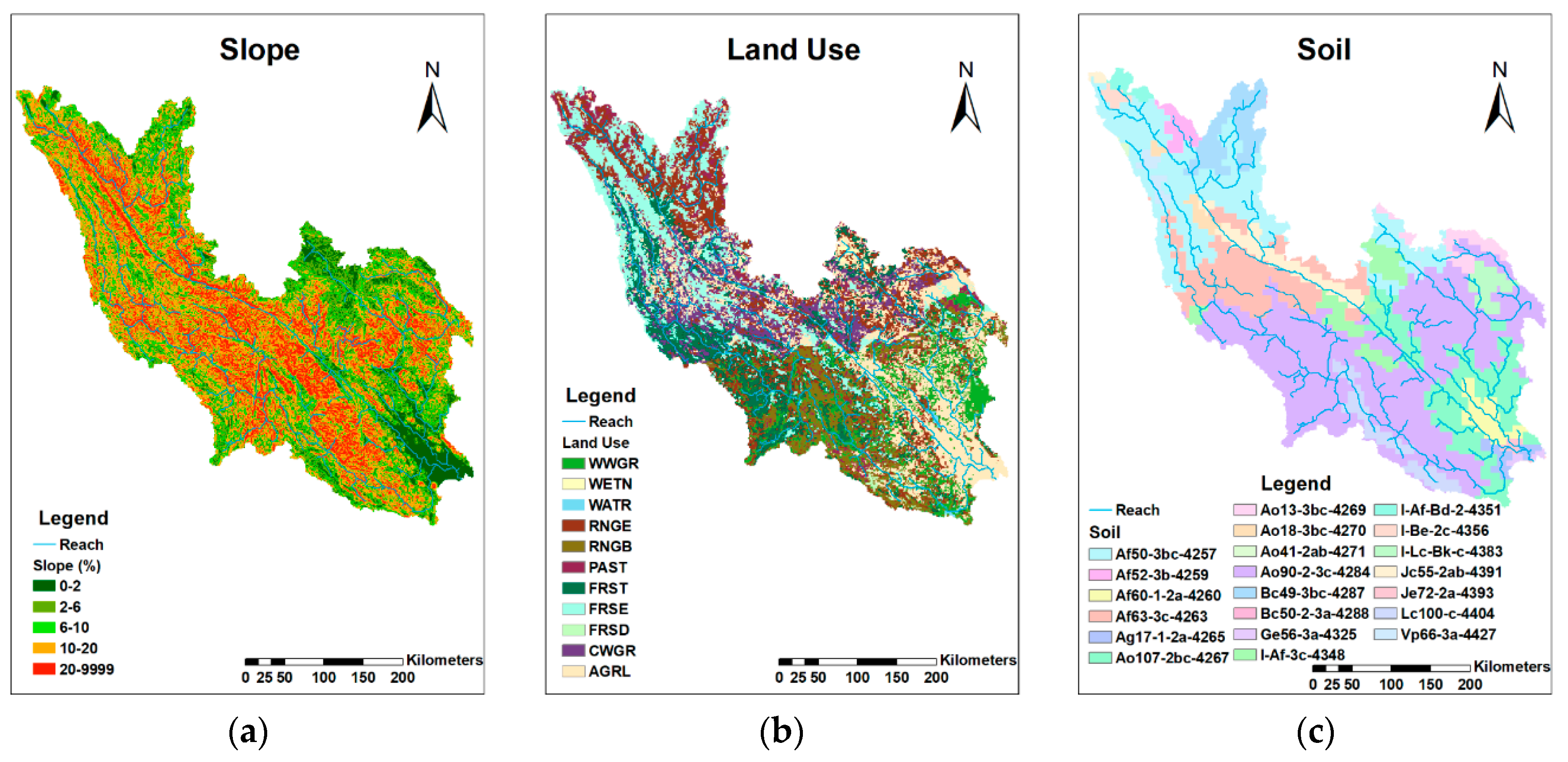
2.3.1. Topography, Land Use and Soil

The landscape slopes were divided into 5 classes by SWAT based on the information from DEM (details are shown in Figure 2a). The dominant lands are forest (27.56%, with 14.65% of evergreen forest (FRSE in SWAT model), 12.49% of mixed forest (FRST) and 0.42% of deciduous forests (FRSD)); agriculture (ARGL, 21.16%); range-grasses (RNGE, 19.94%); wheatgrass (19.57%, with 10.03% of western wheatgrass (WWGR) and 9.54% of crested wheatgrass (CWGR)) (Figure 2b).

There are 21 specific soils in study area (Figure 2c); however, most of them are Acrisols [78].

Resolutions and download links can be found in Table 2.

2.3.2. Meteorological Data

Daily temperature data were obtained from the Global Weather Data in SWAT file format for a given location and time period. These data come from the daily Climate Forecast System Reanalysis (CFSR).

Daily precipitation data was obtained from the Tropical Rainfall Measuring Mission (TRMM, product 3B42 V7), which is a research satellite designed to provide needed information on rainfall by covering the tropical and sub-tropical regions of the Earth. Simons et al. [54] compared several satellite-based precipitation and actual evapotranspiration products in the Red River basin in order to demonstrate that these datasets can be merged to examine hydrological processes before applying a numerical simulation model, and they found that TRMM rainfall product could provide reliable values in both space and time at this basin.

2.3.3. Dam Implementations

SWAT requires basic information, such as date of impoundment, reservoir surface area, emergency volume, principal volume and initial volume. The volume of outflow can be calculated by one of the following methods: measured daily outflow, measured monthly outflow, average annual release rate and controlled outflow with target release. As it is impossible to get the detailed outflow of dams, and in order to avoid the complex conditions of release operations and to enable the model to be applied for future hydrology regime prediction, the average annual release rate method that releases the water whenever the dam volume exceeds the principal spillway volume [57] was selected. A minimum and a maximum average daily releases for the month were limited for the model according to the Q data we collected and to the release information from reference [37].

The six dams localized in Figure 1 were taken into account in the model. Two dams are located on the main stream of the Thao River, around 150 km and 100 km upstream of Lao Cai, respectively; two are on the Da River; and the other two are on the Lo River. However, inside this basin, there are more dams that were put into use [79], or are under construction during simulation period; and these dams are located more in the upper regions and most are with less capacities. Here, the model only took these six dams with large capacity into account, and also they are located closer to the outlet of each tributary, see Table 1.

2.4. Model Set Up

SWAT2012 and ArcGIS10.4 were used. The whole basin was divided into 242 sub-basins and then subdivided into 3812 different HRUs.

Two scenarios were simulated: (1) actual situation and (2) natural situation. Simulation was carried out at three temporal scale (daily, monthly and annually) during an overlapped period, from January 2000 to July 2014.

2.5. Calibration and Validation Process

The model was calibrated at a daily scale using Q and SSC from 1 January 1998 to 31 July 2014 with a two-year warm-up. Parameters were mainly calibrated manually, and some were automatically calibrated by using SWAT-CUP [80]. SWAT-CUP is a tool that allows SWAT users to perform automatic calibrations [81]. Five algorithms are proposed for calibration purpose [80,82]. The SUFI-2 (Sequential Uncertainty Fitting 2) algorithm [82], which can identify appropriate parameters sets in a limited number of iterations, was selected in this study. Calibration of Q was first carried out, followed by SSC.

Observed data of daily Q and SS concentration from 2000 to 2014, obtained from the Vietnam Ministry of Natural Resources and Environment (MONRE) at Lao Cai, Yen Bai, Vu Quang, Hoa Binh and Son Tay stations, were used to calibrate the model. Figure 1 shows the location of each gauge station. Time series plots and statistical methods were used to evaluate the performance of model in simulating Q and SSC.

Values from other references [37,39,43,50,51,53,83,84,85] are used to be validations of the water regime and SSC.

2.6. Model Evaluation

2.6.1. The Coefficient of Determination (R²)

R² describes the proportion of the variance in measured data explained by the model. R² is calculated as follows:

$$R^2=\frac{{{\displaystyle \sum }}_{i=1}^n(O_i-\overline{O})\left(S_i-\overline{S}\right)}{\sqrt{{{\displaystyle \sum }}_{i=1}^n{(O_i-\overline{O})}^2}\sqrt{{{\displaystyle \sum }}_{i=1}^n{\left(S_i-\overline{S}\right)}^2}}$$

(5)

where $O_i$ and $S_i$ are the observed and simulated values, n is the total number of values, $\overline{O}$ is the mean of observed values and $\overline{S}$ is the mean of simulated values.

R² ranges from 0 to 1, with higher values indicating less error variance, and typically values greater than 0.5 are considered acceptable [86].

2.6.2. The Nash–Sutcliffe Efficiency (NSE)

NSE is a normalized statistic that determines the relative magnitude of the residual variance compared to the observed data variance [87], calculated as follows:

$$\mathrm{NSE}=1-\frac{{{\displaystyle \sum }}_{i=1}^n{\left(O_i-S_i\right)}^2}{{{\displaystyle \sum }}_{i=1}^n{\left(O_i-\overline{O}\right)}^2}$$

(6)

NSE ranges from negative infinity to 1.00, with NSE = 1 being the optimal value. A negative value indicates that the mean value of the observed time series would have been a better predictor than the model [88]. NSE values between 0.0 and 1.0 are generally regarded as acceptable levels of performance. Related to the guidelines proposed by Moriasi et al. [86], NSE values above 0.5 are considered as satisfactory in hydrological modeling. Performance ratings for statistics of monthly scale provided by Moriasi et al. [86] are reported in

Table 3. General Performance Ratings for NSE and PBIAS of a Monthly Time Scale [86].

Performance Rating	NSE	PBIAS
		Q	SSC
Very good	0.75 < NSE ≤ 1.00	PBIAS < ±10	PBIAS < ±15
Good	0.65 < NSE ≤ 0.75	±10 ≤ PBIAS < ±15	±15 ≤ PBIAS < ±30
Satisfactory	0.50 < NSE ≤ 0.65	±15 ≤ PBIAS < ±25	±30 ≤ PBIAS < ±55
Unsatisfactory	NSE ≤ 0.50	PBIAS ≥ ±25	PBIAS ≥ ±55

.

2.6.3. The Percent Bias (PBIAS)

PBIAS provides the information of average tendency of the simulated data to be larger or smaller than their observed counterparts. The optimal value is 0.0, with low-magnitude values indicating accurate model simulation. Positive and negative values indicate model underestimation bias and overestimation bias, respectively. Equation is presented as follows:

$$\mathrm{PBIAS}=\frac{{{\displaystyle \sum }}_{i=1}^n\left(O_i-S_i\right)\times 100}{{{\displaystyle \sum }}_{i=1}^n{O}_i}$$

(7)

According to Moriasi et al. [86], these guidelines should be adjusted based on the quality and quantity of measured data, model calibration procedure and evaluation time step.

3. Results

3.1. Q Simulation and Hydrological Assessment

3.1.1. Hydrological Parameters

Table 4. Parameters Used to Calibrate Flow and Suspended Sediment Concentration for Different Basins.

Parameter (Name in Equations)	Input File	Definition	Range	Calibrated Value
OV_N	.hru	Manning’s “n” value for overland flow	0.01–30	0.4
SLSUBBSN	.hru	Average slope length (m)	10–150	×1.2 (relative change)
HRU_SLP	.hru	Average slope steepness (m/m)	–	×0.8
ESCO	.hru	Soil evaporation compensation factor	0–1	0.7
PRF (prf)	.BSN	Peak rate adjustment factor for sediment routing in the main channel	0–2	1
SPCON (Csp)	.BSN	Linear parameter for calculating the maximum amount of sediment that can be re-entrained during channel sediment routing	0.0001–0.01	0.008 (Period 2000–2007) 0.002 (Period 2008–2014)
SPEXP (spexp)	BSN	Exponent parameter for calculating sediment re-entrained in channel sediment routing	1–2	2
ALPHA_BF	.gw	Baseflow alpha factor	0–1	0.02
GW_REVAP	.gw	Groundwater “revap” coefficient	0.02–0.20	0.03
REVAPMN	.gw	Threshold depth of water in the shallow aquifer for “revap” or percolation to the deep aquifer to occur	0–1000	800
RCHGR_DP	.gw	Deep aquifer percolation fraction	0.0–1.0	0
GWQMN	.gw	Threshold depth of water in the shallow aquifer required for return flow to occur	0–5000	600
GW_DELAY	.gw	Groundwater delay time	0–500	16
SOL_AWC	.sol	Available water capacity of the soil layer	0–1	×1.2
USLE_K (KUSLE)	.sol	USLE equation soil erodibility (K) factor	0–0.65	Thao River basin 0.3 Lo River basin 0.2 Da River basin 0.3
CH_COV1 (Kch)	.rte	The channel erodibility factor	−0.05–0.6	Thao River basin: upstream Yen Bai: 0.23; Yen Bai-Son Tay: 0.013 Lo River basin 0.013 Da River basin 0.026
CH_COV2 (Cch)	.rte	Channel cover factor	−0.001–1	1
CH_N2	.rte	Manning’s “n” value for the main channel	−0.01–0.3	0.05
USLE_P (PUSLE)	.mgt	USLE equation agricultural practice factor	0–1	Thao River basin 0.7(agriculture) Lo River basin 0.4(agriculture) Da River basin 0.7(agriculture)
FILTERW	.mgt	Width of edge-of-field filter strip	0–100	Thao River basin 0 Lo River basin 25 Da River basin 0
CN2	.mgt	Initial SCS runoff curve number	35–98	×0.9 (Relative change)
CH_N1	.sub	Manning’s “n” value for the tributary channels	0.01–30	1

presents the calibrated parameters for Q and SSC, and their definitions and ranges. Sensitive hydrological parameters are chosen by literature reviews [64,89,90,91]. Relative change of parameters was controlled within ±20%, and absolute change was done by referring to the aforementioned literatures and theoretical documents [57,81,91,92]. Based on actual information from the MONRE and literatures [50,83], parameters like runoff curve number (CN2), soil evaporation compensation factor (ESCO), available water capacity of the soil layer (SOL_AWC) and parameters related to groundwater (GW_REVAP, REVAPMN, RCHGR_DP, GWQMN, GW_DELAY) were calibrated to fit the actual water balance. Compared to the default values, ESCO was decreased and GW_REVAP was increased to increase the ET; SOL_AWC was increased by 20%; CN2 was decreased by 10%; REVAPMN was increased; and RCHGR_DP and GWQMN were decreased to decrease the surface flow, which accordingly increased the groundwater flow. Other parameters related to hydrological processes were calibrated to fit the baseflow and peaks, and they were interpreted in the following sub-section.

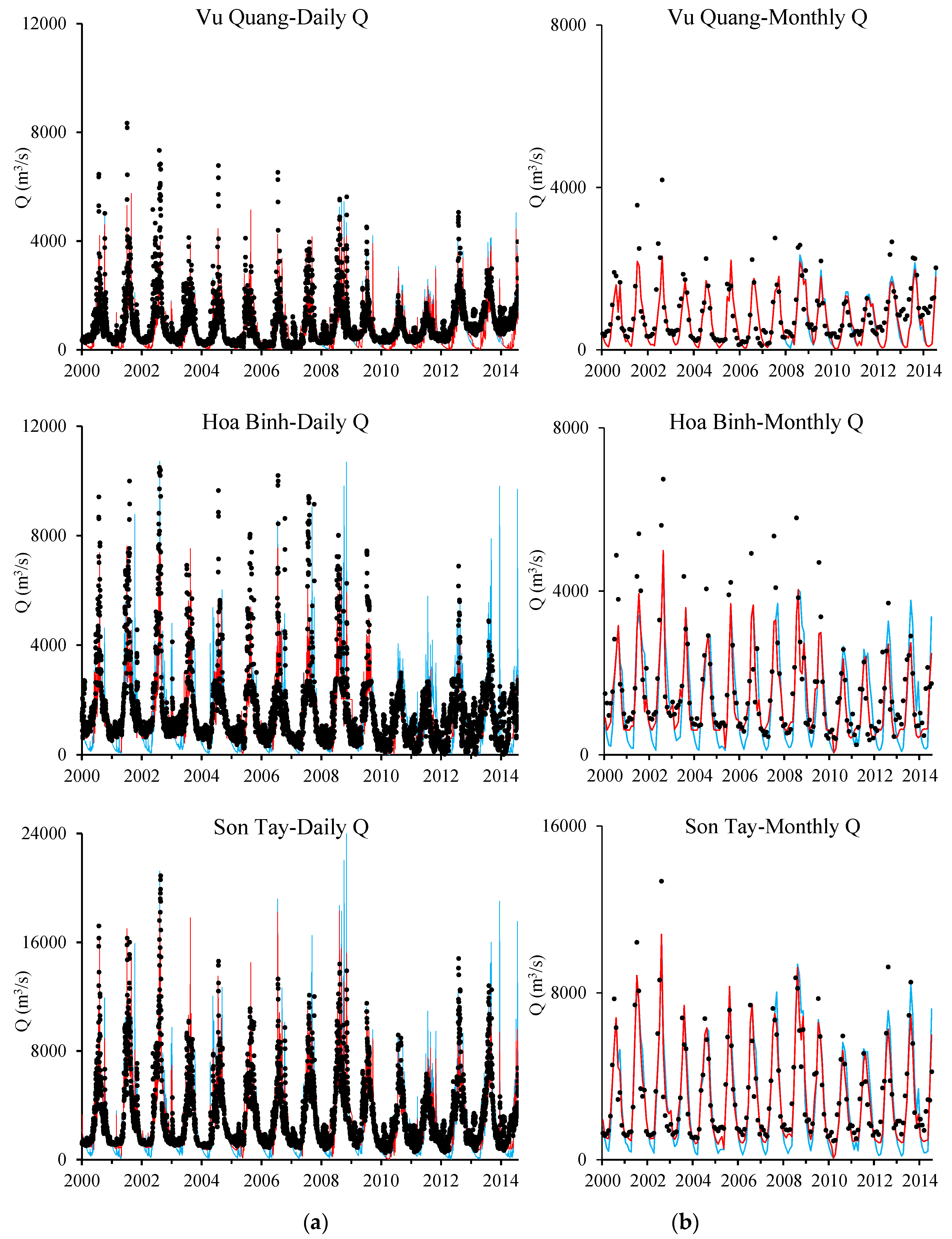
3.1.2. Q simulations

Daily and monthly evaluation statistics are presented in

Table 5. Evaluation Statistics of Observed and Simulated Discharge (Q), Suspended Sediment Concentration (SSC) and Sediment Flux (SF) on Different Time Scales for Each Station.

Constituent	Scale	Statistics	Lao Cai	Yen Bai	Vu Quang	Hoa Binh	Son Tay
Q (m3/s)	Daily	NSE	0.44	0.35	0.38	0.49	0.61
		R2	0.57	0.52	0.45	0.53	0.64
		PBIAS	2.8	−11.2	21.2	18.1	6.0
		p-value	<0.01	<0.01	<0.01	<0.01	<0.01
	Monthly	NSE	0.78	0.78	0.58	0.70	0.85
		R2	0.82	0.88	0.65	0.77	0.86
		PBIAS	2.8	−11.0	21.3	17.9	5.9
		p-value	<0.01	<0.01	<0.01	<0.01	<0.01
SSC (mg/L)	Daily	NSE	0.31	0.23	0.02	0.10	0.19
		R2	0.34	0.30	0.29	0.36	0.34
		PBIAS	−21.4	−28.7	−46.5	−26.3	−28.0
		p-value	<0.01	<0.01	<0.01	<0.01	<0.01
	Monthly	NSE	0.70	0.64	0.24	0.59	0.52
		R2	0.73	0.71	0.55	0.67	0.70
		PBIAS	−21.5	−27.3	−46.8	−26.5	−29.5
		p-value	<0.01	<0.01	<0.01	<0.01	<0.01

. According to the NSE of daily-scale Q simulations, results are acceptable (as NSE > 0) for the stations on the Thao, Lo and Da rivers, and is satisfactory (NSE > 0.5) for Son Tay. At monthly scale, the performance of the model is good, except at Vu Quang station where it is satisfactory. PBIAS values indicates that the model underestimated the discharge for majority stations except for Yen Bai. The absolute values of PBIAS were within 21.3, which is satisfactory. Hence, according to the statistic evaluations, the model performed well simulating Q at both daily and monthly scales.

Figure 3 illustrates the observed and simulated Q comparisons at daily and monthly scale for five stations. Simulated Q shows the same trends as observed Q. At daily scale, the model underestimated base Q at Vu Quang station; and simulated peak Q was underestimated during some floods, especially at Vu Quang and Hoa Binh stations. At Son Tay, at the confluence of the Thao, the Lo and the Da rivers, the simulated Q shows a better agreement with both the base Q and peak Q. At monthly scale, peaks fit well on the Thao River (Lao Cai and Yen Bai) and at Son Tay, while they were underestimated on the Lo (Vu Quang) and the Da River (Hoa Binh); and underestimation on baseflow are only largely noticeable at Vu Quang on monthly scale.

3.2. SSC Simulation

3.2.1. Calibration of SSC

As shown in Section 2.2.3, two groups of parameters were considered, and their calibrated values are shown in Table 4.

A first group of parameters related to landscape processes are involved in Equation (1). Among these parameters, USLE_K and USLE_P are sensitive to soil erosion. Due to the soil characteristics (poor stability and erosion resistance), the Thao and Da basins are more vulnerable to soil erosion [47]. Therefore, USLE_K of the Thao and Da basins (0.3) were higher than that of the Lo basin (0.2). The agricultural practice factor, USLE_P, is defined as the ratio of soil loss with a specific agricultural practice (such as contour tillage, strip cropping on the contour and terrace systems) to the corresponding loss with up-and-down slope culture [57]. In the Thao and Da basins, contour tillage and terrace are common in mountainous regions, such as in Yuanyang County in China and Sa Pa in Vietnam. In the Lo basin, industrial crops and rice paddy are common because of its lower slope. Therefore, referring to the values in accordance with different slopes, 0.7 was set for USLE_P for the agriculture land use in Thao and Da basins and 0.4 for the agriculture land use in the Lo basin. Sediment yield from landscape can be lagged and trapped routed through grassed waterway and vegetative filter strips before reaching the stream channel. In the Lo basin, edge-of-field filter strips, which could be cultivated lands, grass and bush, are widely distributed along the river, while in the other two sub-basins, there are no such filter strips due to the steep valley. From measurements on Google Earth views, the width can range from 20 m to more than 300 m. Combining filed investigation, expertise from local researchers and calibrations from model, a width edge-of-field filter strips of 25 m was set for FILTERW in the Lo basin, which is considered as an average and approached value.

A second group of parameters, relating to in-stream SS process (deposition and aggradation), is required for Equation (2), which is more familiar with a power function sediment rating curve as:

$$\mathrm{SSC}=\mathsf{\alpha }{Q}^{\beta }$$

(8)

where α and β are regression coefficients.

SPCON, SPEXP and PRF are the key parameters that control the maximum concentration of sediment that can be transported by the flow. SPCON corresponds to α and it is a proxy to express the river bed erodibility; the PRF parameter modulates the SPCON behavior, and the default value of PRF often equals 1. SPEXP corresponds to β to express the erosive power of the river [39]. According to Asselman [22], a low α-value coupled to a high β-value are characteristic of river sections with little sediment transport at low discharge. During the study period (2000–2014), the Red River basin encompassed large ranges of measured SSC values: 6.9–18,300 mg/L in the Thao River; 0.6–3350 mg/L in the Lo River; 0.4–481 mg/L in the Da River; and 2.1–4100 mg/L in the Red River at Son Tay. The Red River transports little sediment at low discharge, and a low α-value and a high β-value should be set for this basin. Therefore, SPEXP was set to 2, and SPCON was calibrated after PRF and SPEXP were fixed. A value of 0.008 was set to SPCON before dam implementations, from 2000 to 2007. After dam implementations, the coarser particles were retained by dams, and the particle size distribution was affected downstream, leading to a change in the channel erodibility. Then, the dynamics of downstream suspended sediment transport decreased. Due to the complexity of dam implementations over the study period, we assume that the hydrodynamics of SS transport by the rivers in the Red River changed after 2007. Indeed, the Nansha dam is operational since 2008, and the Madushan dam construction started by the end of 2008; then Tuyen Quang is operational since 2008. Therefore, a lower value of SPCON (0.002) was set for the period from 2008. In Equation (4), two parameters are related to degradation process: CH_COV1 is the channel erodibility factor, and CH_COV2 is the channel cover factor channel. CH_COV1 is a function of properties of the bed or bank materials, and is conceptually similar to the soil erodibility factor used in the USLE equation [57]. CH_COV2 was set to 1, which means there is no vegetative cover on channel.

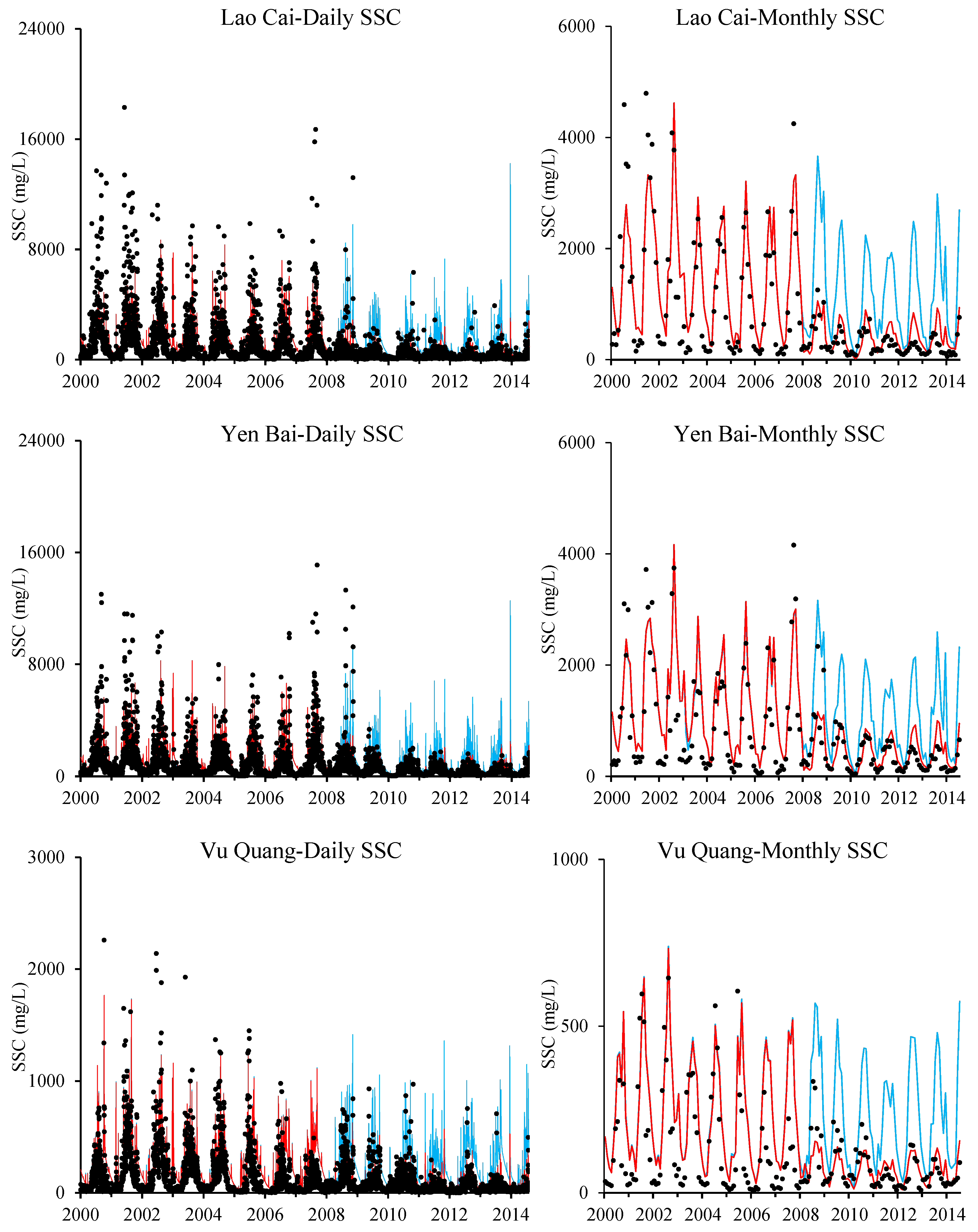
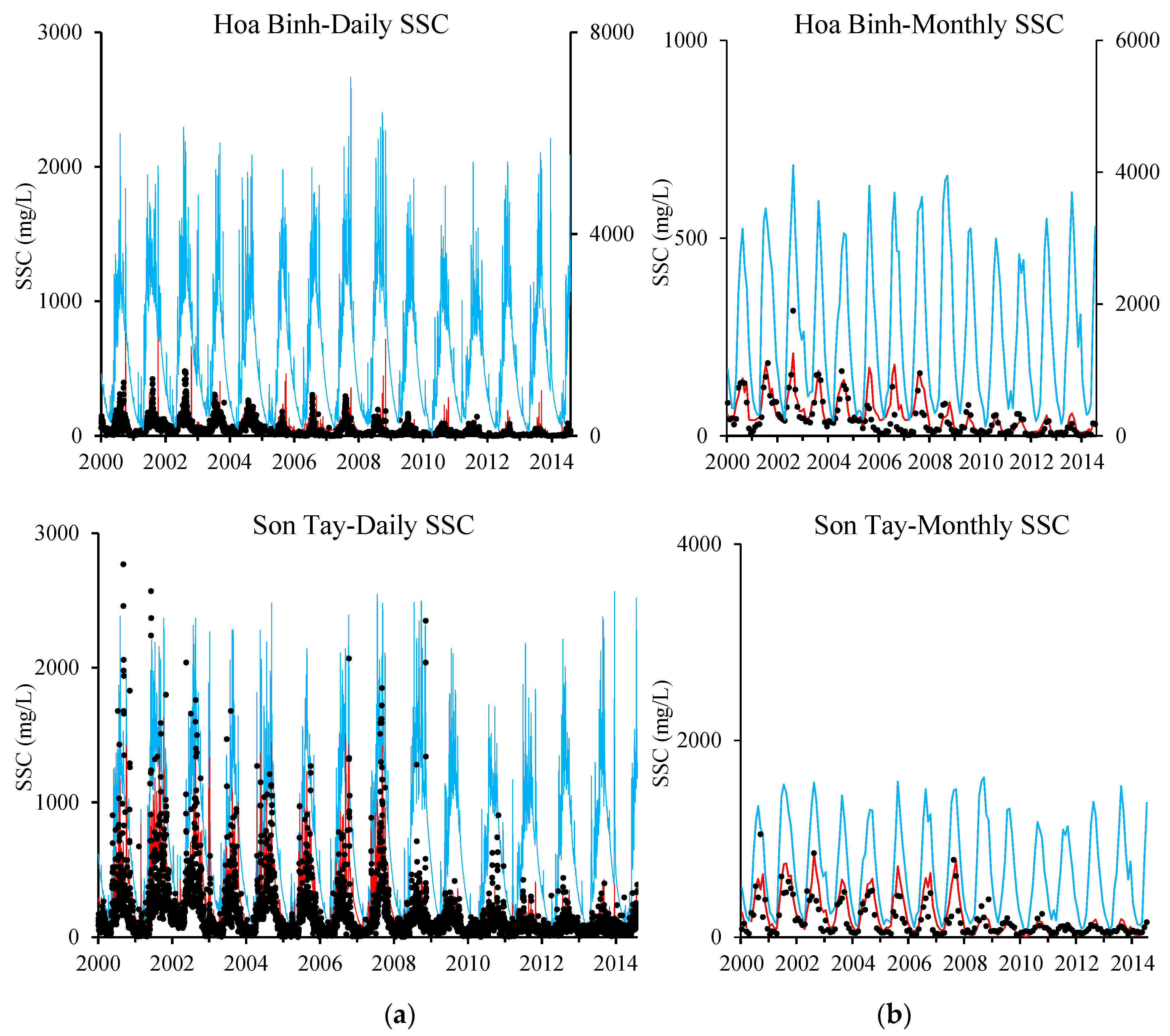
3.2.2. SSC Simulations

Statistics evaluation of SSC simulations at daily and monthly scales are shown in Table 5. According to the general evaluation of NSE and R², SSC simulations at these 5 stations are acceptable (NSE > 0, R² > 0). From the general performance ratings at monthly scale recommended by Moriasi et al. [86], Lao Cai, Yen Bai, Hoa Binh, and Son Tay stations presented satisfactory and good performance; and for the Vu Quang station, though the NSE is not satisfactory, PBIAS is within the satisfactory range. PBIAS values indicate that the model overestimated SSC for all stations. Maximum absolute values of PBIAS were 46.8%, which is still satisfactory following the Moriasi criteria (Table 5). Therefore, according to the statistic evaluations, the model simulated SSC at a satisfactory range.

The simulated SSC is in the range of the observed SSC during the simulation period, and showed similar trends to observations at the five stations (Figure 4). However, the magnitude of simulated SSC peaks was either underestimated or overestimated during some periods. For example, daily simulated SSC peaks were generally underestimated before 2009 at Lao Cai, Yen Bai, Hoa Binh, and Son Tay, but monthly SSC peaks fit well with observed monthly peaks. Conversely, some monthly simulated SSC peaks were overestimated, such as in 2011–2014 at Lao Cai, 2012–2014 at Yen Bai, 2006–2007 at Vu Quang, 2005 at Hoa Binh, and 2003–2006 at Son Tay.

3.3. Impacts of Climate Variability and Dams

In order to identify and separate the impacts of climate variability and dams, analysis was carried out based on the annual mean Q and SSC of natural conditions (without dams) and actual conditions.

3.3.1. Impacts on Q

Table 6. Annual mean discharge (Q) from 2000 to 2013 and the multi-year annual mean Q of 2000–2007 (before new dams’ constructions) and 2008–2013 (after new dams’ constructions). Variation tendency of annual mean Q from 2000–2013 and 2008–2013. Impact percentages of climate variability and dams.

Q (m3 s−1)	Lao Cai		Yen Bai		Vu Quang		Hoa Binh		Son Tay
	NC*	AC*	NC*	AC*	NC*	AC*	NC*	AC*	NC*	AC*
2000	551	551	757	757	694	694	1318	1370	2910	2963
2001	778	778	1013	1013	803	803	1645	1613	3656	3624
2002	741	741	971	971	733	733	1687	1688	3489	3491
2003	796	796	1029	1029	794	794	1677	1619	3696	3637
2004	520	520	745	745	670	670	1373	1364	2936	2928
2005	405	405	644	644	717	717	1217	1198	2713	2694
2006	476	476	666	666	651	651	1455	1456	2920	2921
2007	605	605	793	793	675	675	1521	1523	3123	3125
2008	693	693	995	995	975	1006	1810	1774	4019	4015
2009	406	406	623	623	722	763	1240	1391	2736	2928
2010	348	348	516	516	567	567	1110	849	2304	2043
2011	365	349	574	557	654	656	1221	1034	2603	2401
2012	351	352	566	568	723	717	1203	1093	2669	2556
2013	420	420	646	645	763	760	1452	1101	3066	2712
2000–2007	609	609	827	827	717	717	1487	1479	3180	3173
2008–2013	430	428	653	651	734	745	1339	1207	2900	2776
Tendency 2000–2013 (m3 s−1 year−1) (related R**)	−27.4 (0.70)	−27.7 (0.70)	−28.5 (0.66)	−28.8 (0.66)	−2.7 (0.12)	−2.2 (0.09)	−22.2 (0.43)	−40.8 (0.62)	−51.5 (0.44)	−69.9 (0.54)
Tendency 2008–2013 (m3 s−1 year−1) (related R**)	−43.1 (0.61)	−43.5 (0.61)	−53.1 (0.57)	−53.5 (0.57)	−27.7 (0.38)	−36.6 (0.46)	−51.1 (0.37)	−116.3 (0.66)	−133.3 (0.42)	−207.8 (0.57)
Impacts of climate and dams	30%		21%		−4%		18%		13%
Impacts of climate	29%		21%		−2%		10%		9%
Impacts of dams	0.4%		0.3%		−2%		8%		4%

*NC, natural conditions; AC, actual conditions; R**, linear regression.

presents the annual mean Q in each year and the variation tendency of each station under different scenarios.

For the whole study period, under natural conditions, the biggest decreasing tendency of Q is at Son Tay station, followed by Yen Bai station, and least decreasing tendency is at Vu Quang station; under actual conditions, the annual mean Q decreased at almost the same degree at most stations compared with those under natural conditions, except at Hoa Binh station and consequently at Son Tay. During 2008–2013, the natural annual mean Q showed bigger decreasing tendencies compared to 2000–2013; actual annual mean Q decreased faster on the Thao River and Da River.

Decreasing rate was calculated from comparison between 2000–2007 and 2008–2013. The actual annual mean Q during 2008–2013 at Son Tay reduced to 13% of that during 2000–2007 under natural conditions; among them 9% was reduced by the climate variability, and 4% was caused by the dams upstream. Among the three tributaries, the Thao River shows little impacts of dams; the Vu Quang station on the Lo River actually shows positive impacts of climate and dams; the Hoa Binh on the Da River shows almost equal impacts of climate and dams.

3.3.2. Impacts on SSC

Table 7. Annual mean suspended sediment concentration (SSC) from 2000 to 2013 and the multi-year annual mean SSC of 2000–2007 (before new dams’ constructions) and 2008–2013 (after new dams’ constructions). Variation tendency of annual mean SSC from 2000 to 2013 and 2008 to 2013. Impact percentages of climate variability and dams.

SSC (mg/L)	Lao Cai		Yen Bai		Vu Quang		Hoa Binh		Son Tay
	NC*	AC*	NC*	AC*	NC*	AC*	NC*	AC*	NC*	AC*
2000	1435	1435	1281	1294	241	238	1549	80	682	321
2001	1860	1860	1660	1671	279	276	1809	90	830	396
2002	1815	1815	1669	1686	287	283	1836	88	780	362
2003	1915	1915	1714	1726	277	273	1852	90	848	400
2004	1383	1383	1244	1257	221	216	1586	76	684	307
2005	1196	1196	1141	1166	236	231	1446	71	624	296
2006	1308	1308	1151	1167	225	222	1636	80	679	289
2007	1498	1498	1338	1347	246	244	1717	84	731	320
2008	1727	511	1512	576	286	94	1916	33	800	107
2009	1206	360	1068	438	224	67	1486	22	626	77
2010	1018	342	983	385	208	65	1394	19	554	77
2011	1166	388	1028	428	208	64	1455	18	612	75
2012	1085	381	1005	429	240	69	1384	20	592	78
2013	1243	409	1140	471	227	66	1597	22	655	83
2000–2007	1551	1551	1400	1414	251	248	1679	83	732	336
2008–2013	1241	398	1122	455	232	71	1539	23	640	83
Tendency 2000–2013 (mg L−1 year−1) (related R**)	−48.9 (0.68)	−132.9 (0.89)	−42.9 (0.69)	−111.5 (0.89)	−3.5 (0.53)	−19.9 (0.90)	−21.3 (0.49)	−6.7 (0.89)	−13.7 (0.62)	−28.9 (0.90)
Tendency 2008–2013 (mg L−1 year−1) (related R**)	−75.3 (0.56)	−11.5 (0.36)	−57.2 (0.54)	−14.5 (0.41)	−7.0 (0.45)	−3.7 (0.62)	−52.6 (0.49)	−1.7 (0.58)	−22.1 (0.48)	−3.5 (0.53)
Impacts of climate and dams	74%		68%		72%		99%		89%
Impacts of climate	20%		20%		8%		8%		13%
Impacts of dams	54%		48%		64%		90%		76%

*NC, natural conditions; AC, actual conditions; R**, linear regression.

presented the annual mean SSC in each year and the variation tendency of each station under different scenarios.

For the whole study period, the SSC under natural conditions showed a biggest decreasing tendency in the Thao River, followed by the Da River, and least decreasing tendency was in the Lo River; under actual conditions, the annual mean SSC decreased more severely at most stations than under natural conditions, except at Hoa Binh station. During 2008–2013, the natural annual mean SSC showed bigger decreasing tendencies compared to 2000–2013; actual annual mean SSC decreased faster on the Thao River, then on the Lo and Da River.

The actual annual mean SSC during 2008–2013 at Son Tay reduced to 89% of that during 2000–2007 under natural conditions; among the 89%, 13% was reduced because of the climate variability, and 76% was caused by the dams upstream. Among the three tributaries, Hoa Binh and Vu Quang are influenced more by the dams while the Thao River basin is influenced more by the climate variability.

4. Discussion

4.1. Uncertainties

4.1.1. Uncertainties of Hydrology Modeling

Base flow alpha factor (ALPHA_BF), which was sensitive for baseflow, was suggested by the Baseflow Filter Program [93,94] to 0.02. Other parameters associated with groundwater and baseflow in Table 4 were calibrated by SWAT-CUP under the range recommended by SWAT theoretical documentation [57]. Hydrological parameters were calibrated at the whole basin, while these three sub-basins are different in hydrogeology, soil and land use. This might cause the deviations on the baseflow estimation at Vu Quang in the Lo sub-basin. In addition, downstream of the Red River system, especially in the Lo River sub-basin, agriculture activities are active and intensive, and there are many complex irrigation systems. Water is extracted for irrigation from the main stream and delivered to ditch and canal, or water can be taken from one river and drainage to another river. This might contribute to uncertainties for the baseflow at the Lo River sub-basin.

The simulation of the peak Q on the Thao River is more satisfactory than on the Lo and Da Rivers. The underestimation during flood season most probably results from the errors in either precipitation estimates or uncertainties in observed flow. Le et al. [95] indicated that due to the coarse resolution, TRMM rainfall products cannot adequately capture extreme rainfall values. The scatter plots of precipitation from rain gauge stations versus TRMM products from the study of Liu et al. [96] and Simons et al. [54] also showed that high and intensive rainfall is underestimated by TRMM. Discharge of high floods is usually extrapolated by rating curve, which can cause uncertainties.

As shown in Table 1, two dams (the Thac Bac dam and the Hoa Binh dam) were implemented before the beginning of the simulation period (2000), and other dams started to operate since 2008. Upstream of Lao Cai, China has been building cascade power stations, and the first one named Nansha dam started to be built on February 2006 and to work on November 2007, and the second one named Madushan dam began to be constructed downstream in December 2008 and started to work in December 2010. Upstream of the Lo River, the Tuyen Quang dam has been put into function since March 2008. Furthermore, there are at least 10 more smaller dams that can be found on Google Earth in Vietnam; however, when these dams were operated is difficult to figure out. Upstream of Hoa Binh station, the Son La dam was implemented on December 2010, and at least 8 more dams can be seen on Google Earth in Vietnam. Certainly, many dams can be also found in Chinese part for both the Lo and Da River on Google Earth. Liu et al. [97] pointed that hydrological forecasting effectiveness and accuracy would be affected greatly by the construction and operation of the cascade reservoirs. It is difficult for the model to precisely simulate the complex operation of dam discharge, which depends on the arriving water volume, on the downstream water regime, and also on the variation of irrigation storage. Complexities can be seen in the base Q from 2010 to 2014 at Hoa Binh station. Besides, as mentioned before, there are many small dams and irrigation systems that were not taken into account in this model; this also contributed to deviations in simulations. These uncertainties of anthropogenic influences, especially the dams, caused deviation on calibrations, such as the base Q of 2010–2014 at Vu Quang station. Nevertheless, monthly simulated Q at Vu Quang is still satisfactory with NSE of 0.58, R² of 0.65, and PBIAS of 21.3.

4.1.2. Uncertainties of Suspended Sediment Modeling

From the daily simulation, we can notice that deviations mainly occur during large floods. Some studies [89,98] showed that modeling might underestimate SSC during high and intensive rainfall. This underestimation can come from the landscape component when using a runoff factor instead of rainfall energy factor, or/and from the channel component where particle-size elements are neither tracked nor considered in the physical processes in floodplains. As already explained, uncertainties can also be related to satellite rainfall estimations from TRMM, or/and from data measurement and sampling strategy.

The SWAT model used a simplified version of Bagnold [77] stream power equation to calculate the maximum amount of sediment that could be transported in a stream segment. However, this algorithm does not keep track of particle size distribution of elements that pass through the channel, and all are assumed to be of silt size. Further, the channel erosion is not partitioned between stream bank and stream bed, and deposition is assumed to occur only in the main channel; flood plain sediment deposition is also not modeled separately [57]. Therefore, this simplification can cause deviations for sediment routing.

4.2. Water Balance and Yield

The average annual rainfall during the simulation period, using the TRMM data of precipitation, was 1493.6 mm, of which 53% (787.7 mm) was taken away through evapotranspiration (ET) and 47% fed the stream flow. The average potential evapotranspiration (ETP) predicted by the model was 1293 mm. Le et al. [83] used different methods to predict the ETP of this basin, and gave a range from 960 to 1289 mm for the period 1964–2008, while the actual evapotranspiration (ETA) was estimated from 771 to 1186 mm. For streamflow, the model estimated a water yield of 696.8 mm, which is close to the real water yield, 669 mm, calculated from the data collected from the Vietnam Ministry of Natural Resources and Environment (MONRE) during the same period. Among the simulated water yield, surface runoff accounted for 39% while the lateral flow accounted for 3% and the groundwater accounted for 58%. This result is in agreement with Le [50] and Bui et al. [84]. Le [50] indicated that the groundwater resource in Vietnam is abundant, accounting for around 58% of total streamflow, and is a critical component river flow during the dry season. Bui et al. [84] underlined on a typical small steep basin of Northern Vietnam that the deep infiltration is a key factor of the hydrological pattern in spite of the strong slope gradient above 30%. Therefore, the model provided a credible simulation for each component.

Simulated mean annual Q during study period at Lao Cai, Yen Bai, Vu Quang, Hoa Binh, and Son Tay are 16.7, 23.7, 23.0, 43.0 and 94.7 km³, respectively, suggesting that the Thao River and the Lo River account for nearly 54.6% of the total volume of Son Tay, while the Da River accounts for 45.4%. According to the references and data we collected from the MONRE, the mean annual runoff volume upstream in China from 1956–2000 was 14.6 km³, ranging from 8.4 km³ in 1980 to 24.6 km³ in 1971 [53], and the simulation at Lao Cai is within this range; and at Son Tay from 1960 to 2010, the mean annual runoff was 105.7 km³, with a minimum value of 80.2 km³ in 2010, and a maximum of 158.4 km³ in 1971. Other studies indicated that the Da River is the main flow contribution to the Son Tay, accounting for 50–57% of the total discharge [37,39,85]. Simulations are thus in good agreement with other studies and with the observed data.

Hence, combining with the satellite date, the model performed well at both water balance and yield.

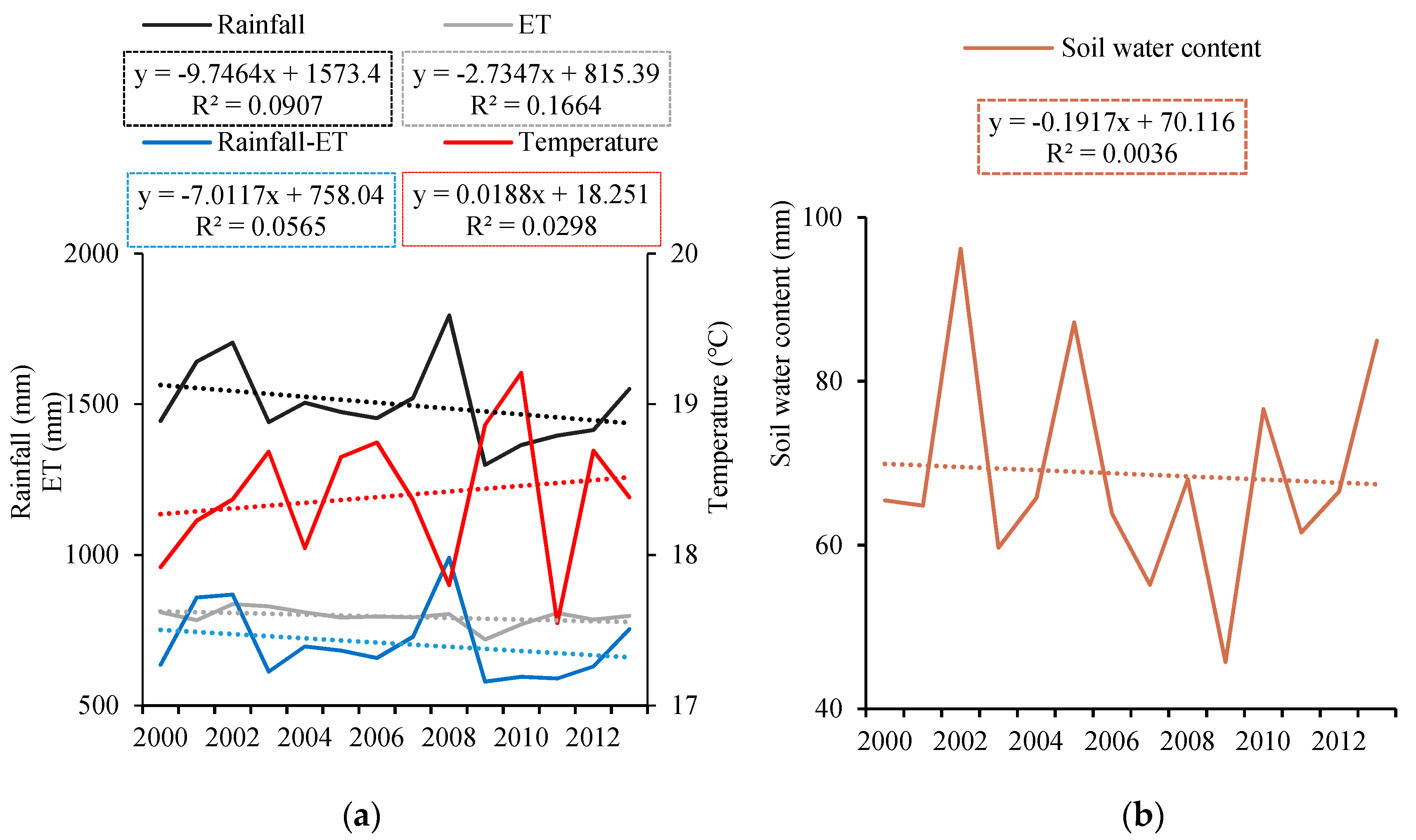
4.3. Natural Conditions Effects

In order to find out the driving factors that decrease Q under natural conditions, we analyzed the tendency of the annual mean rainfall, evapotranspiration (ET), and temperature of the whole basin. From Figure 5, we can see that the annual mean rainfall shows decreasing tendencies while temperature shows a contrary tendency. ET can come from the water body, the plants and the soil, and it can be influenced by many factors, such as geomorphology, climate, soil water content, vegetation cover, etc. Ignoring the possible changes of geomorphology and vegetation cover, we checked the variation of soil water content and found that it showed a decreasing tendency though its decreasing rate is smaller than the one of ET (Figure 5b). Not taking into account the runoff loses, the available water yield should theoretically equal the difference between rainfall and ET. We can find in Figure 5a that the difference between rainfall and ET shows a decreasing trend, which might indicate that the average annual water yield decreases. During the study period, the annual mean rainfall reduces by 9%, ET reduces by 5%, and temperature increases by 1%. These changes result a 13% decrease of available water with a 4% decrease of soil water content.

Table 6 shows that the main impact factor is not the same in different sub-basins. This can relate to the regional climate characteristics. From the study of Le et al. [37], among these three sub-basins, the mean annual rainfall was highest for the Thao sub-basin, followed by the Da sub-basin, and then the Lo sub-basin. Therefore, the different Q variation rates of each sub-basin can relate to the distribution of rainfall, and the decrease of the rainfall might affect the Thao basin most, resulting a biggest Q decreasing rate among the three tributaries.

Different SSC decreasing rates relate to the different soil erosion rates under different rainfall intensity of each sub-basin. As described in Section 3.2.1, the Thao and the Da basin are more vulnerable to soil erosion; the possible decrease in rainfall might have much less impacts on soil erosion in these two sub-basins than in the Lo basin.

In our study, it is impossible and difficult for us to get all the information of all the dams in this large-scale basin, and take all of them into account in this model. Therefore, this model cannot strictly represent the natural conditions. However, some of the dams locate quite upstream of the Da and Lo tributaries and are with smaller capacities, and these reasons can make them have much less impact on the SSC at the outlet of each tributary. Hence, removing the 6 dams that we considered in the model might maximally reflect the natural conditions.

Land use changes were not taken into account. However, land use changes have been proved to have effects on soil erosion [99]. Therefore, it would be interesting to take the land use changes into account in the future.

4.4. Impacts of Dams

Dams show different degrees of impacts on both Q and SSC. Due to the big capacity of Hoa Binh dam, it shows bigger regulating effect on downstream flow than other dams. Liu et al. [97] addressed that the impact of the dam on runoff increased with the dam capacity. However, even though the Hoa Binh dam has a big capacity, its impact on Q is small. This result is in agreement with the study from Dang et al. [39] who found that there was little or no change of Q before and after the Hoa Binh dam.

Previous studies [39,40,43] estimated the impacts on SS from dams before 2011 based on the measurements. Dang et al. [39] and Vinh et al. [43] mainly focused on the effect of the Hoa Binh dam, and Lu et al. [40] also considered the Thac Ba dam, the Tuyen Quang dam, and the Son La dam. We extended the time period to 2013 and also took the dams in China into account. After 2008, at Lao Cao and Yen Bai station, the actual annual mean SSC reduced to 74% and 68% of that during 2000–2007, among which 54% and 48% are due to the dam effects, respectively. With the accumulation impacts from old dams and new dams, at Vu Quang and Hoa Binh, the actual annual mean SSC reduced to 72% and 99% of that during 2000–2007, among which 64% and 90% are due to the dam effects, respectively. At Son Tay station, the outlet of the continental basin, the annual mean SSC reduced to 89% of that under natural conditions during 2000–2007, and 76% of this 89% was caused by the dams upstream. With more dams to be put into use, the SSC at Son Tay might continue to decrease, and this might influence the downstream water system.

5. Conclusions

This is the first study trying to use a modeling approach to analyze hydrology regime and suspended sediment concentration at a daily scale for a long period in the Red River basin, including considering the successive implementations of dams all along the period. The SWAT model provided some insights on discharge and suspended sediment concentration at daily and monthly scales, respectively, in such a large basin. This study allowed us to understand, characterize, and quantify the discharge and suspended sediment concentration with spatial and temporal variations. What is more, using a modeling approach helped us to separate the impacts from climate variability and anthropogenic impacts. However, some improvements are needed, such as dam information and management, observed rainfall data, discharge and suspended sediment dataset of more stations and longer period, high frequency dataset, to gain a better estimation and understanding of the impacts of climate variability and human interferences.

Under the impacts of both climate variability and dams, the Q and SSC show a decreasing trend. However, climate variability and dams have different influence degrees in different sub-basins. The decrease of Q is more related to climate variability while the decrease of SSC is more related to impacts of dams. The annual mean rainfall of the whole basin decreased 9%, evapotranspiration decreased 5%, and temperature increased 1%; which consequently resulted a 4% decrease on soil water content and a 13% decrease of available water for the whole basin. With the accumulated impacts from three tributaries, at the outlet, Son Tay, from 2008 to 2013, the Q decreased to 13% of that under natural conditions of 2000–2007, and climate variability caused 9% decrease and dams caused 4%; SSC decreased to 89% of that under natural conditions of 2000–2007, and 13% came from the impacts of climate and 76% was decreased by the dams.

With more dams to be implemented in this basin both in Chinese and Vietnamese part, sediment retention would consequently increase, which could subsequently influence the transport of associated matters, such as nutrients, metals, and pesticide, and also the habitats downstream. Based on this study, future studies of nutrients, metal, and pesticide transports and quantification can be carried out by using this new tool. In addition, more scenarios of the global changes, such as land use changes and climate changes in the future and their impacts on hydrology and suspended sediment could be quantified by using the model implemented.

References

1. Mekonnen, M.M.; Hoekstra, A.Y. Four billion people facing severe water scarcity. Sci. Adv. 2016, 2, e1500323. [Google Scholar] [CrossRef] [PubMed]
2. Global Risks 2015, 10th ed.; World Economic Forum: Geneva, Switzerland, 2015.
3. Kunz, M.J.; Wüest, A.; Wehrli, B.; Landert, J.; Senn, D.B. Impact of a large tropical reservoir on riverine transport of sediment, carbon, and nutrients to downstream wetlands. Water Resour. Res. 2011, 47, W12531. [Google Scholar] [CrossRef]
4. Lal, R.; Kimble, J.; Levine, E.; Stewart, B.A. Soils and Global Change; CRC Press: Boca Raton, FL, USA, 1995. [Google Scholar]
5. Nijssen, B.; O’donnell, G.M.; Hamlet, A.F.; Lettenmaier, D.P. Hydrologic sensitivity of global rivers to climate change. Clim. Chang. 2001, 50, 143–175. [Google Scholar] [CrossRef]
6. Arnell, N.W. Climate change and global water resources. Glob. Environ. Chang. 1999, 9, S31–S49. [Google Scholar] [CrossRef]
7. Thi Ha, D.; Ouillon, S.; Van Vinh, G. Water and Suspended Sediment Budgets in the Lower Mekong from High-Frequency Measurements (2009–2016). Water 2018, 10, 846. [Google Scholar] [CrossRef]
8. Watson, R.T.; Noble, I.R.; Bolin, B.; Ravindranath, N.H.; Verardo, D.J.; Dokken, D.J. The Intergovernmental Panel on Climate Change (IPCC) Special Report on Land Use, Land-Use Change, and Forestry; Cambridge University Press: Cambridge, UK, 2000. [Google Scholar]
9. FAO. The State of the World’s Land and Water Resources for Food and Agriculture (SOLAW)—Managing Systems at Risk; The Food and Agriculture Organization of the United Nations: Abingdon, UK; Earthscan: New York, NY, USA, 2011; ISBN 9781849713269. [Google Scholar]
10. Valentin, C.; Agus, F.; Alamban, R.; Boosaner, A.; Bricquet, J.P.; Chaplot, V.; de Guzman, T.; de Rouw, A.; Janeau, J.L.; Orange, D.; et al. Runoff and sediment losses from 27 upland catchments in Southeast Asia: Impact of rapid land use changes and conservation practices. Agric. Ecosyst. Environ. 2008, 128, 225–238. [Google Scholar] [CrossRef]
11. Chen, J.; Shi, H.; Sivakumar, B.; Peart, M.R. Population, water, food, energy and dams. Renew. Sustain. Energy Rev. 2016, 56, 18–28. [Google Scholar] [CrossRef]
12. Zimmerman, J.B.; Mihelcic, J.R.; Smith, J. Global Stressors on Water Quality and Quantity. Environ. Sci. Technol. 2008, 42, 4247–4254. [Google Scholar] [CrossRef] [PubMed]
13. Hecht, J.S.; Lacombe, G.; Arias, M.E.; Dang, T.D.; Piman, T. Hydropower dams of the Mekong River basin: A review of their hydrological impacts. J. Hydrol. 2019, 568, 285–300. [Google Scholar] [CrossRef]
14. Dams and Development: A New Framework for Decision-Making; The World Commission on Dams: London UK, 2000.
15. Lehner, B.; Liermann, C.R.; Revenga, C.; Vörösmarty, C.; Fekete, B.; Crouzet, P.; Döll, P.; Endejan, M.; Frenken, K.; Magome, J.; et al. High-resolution mapping of the world’s reservoirs and dams for sustainable river-flow management. Front. Ecol. Environ. 2011, 9, 494–502. [Google Scholar] [CrossRef]
16. Zarfl, C.; Lumsdon, A.E.; Berlekamp, J.; Tydecks, L.; Tockner, K. A global boom in hydropower dam construction. Aquat. Sci. 2015, 77, 161–170. [Google Scholar] [CrossRef]
17. Van Manh, N.; Dung, N.V.; Hung, N.N.; Kummu, M.; Merz, B.; Apel, H. Future sediment dynamics in the Mekong Delta floodplains: Impacts of hydropower development, climate change and sea level rise. Glob. Planet. Chang. 2015, 127, 22–33. [Google Scholar] [CrossRef]
18. Vörösmarty, C.J.; Meybeck, M.; Fekete, B.; Sharma, K.; Green, P.; Syvitski, J.P.M. Anthropogenic sediment retention: Major global impact from registered river impoundments. Glob. Planet. Chang. 2003, 39, 169–190. [Google Scholar] [CrossRef]
19. Syvitski, J.P.M.; Vörösmarty, C.J.; Kettner, A.J.; Green, P. Impact of humans on the flux of terrestrial sediment to the global coastal ocean. Science 2005, 308, 376–380. [Google Scholar] [CrossRef]
20. Syvitski, J.P.; Morehead, M.D.; Bahr, D.B.; Mulder, T. Estimating fluvial sediment transport: The rating parameters. Water Resour. Res. 2000, 36, 2747–2760. [Google Scholar] [CrossRef]
21. Zhang, S.; Chen, D.; Li, F.; He, L.; Yan, M.; Yan, Y. Evaluating spatial variation of suspended sediment ratingcurves in the middle Yellow River basin, China. Hydrol. Process. 2018, 32, 1616–1624. [Google Scholar] [CrossRef]
22. Asselman, N.E. Fitting and interpretation of sediment rating curves. J. Hydrol. 2000, 234, 228–248. [Google Scholar] [CrossRef]
23. Achite, M.; Ouillon, S. Suspended sediment transport in a semiarid watershed, Wadi Abd, Algeria (1973–1995). J. Hydrol. 2007, 343, 187–202. [Google Scholar] [CrossRef]
24. Daniel, E.B.; Camp, J.V.; LeBoeuf, E.J.; Penrod, J.R.; Dobbins, J.P.; Abkowitz, M.D. Watershed Modeling and its Applications: A State-of-the-Art Review. Open Hydrol. J. 2011, 5, 26–50. [Google Scholar] [CrossRef]
25. Islam, Z. A Review on Physically Based Hydrologic Modeling; University of Alberta: Edmonton, AB, Canada, 2011; Available online: https://www.researchgate.net/publication/272169378_A_Review_on_Physically_Based_Hydrologic_Modeling (accessed on 3 May 2019).
26. Devia, G.K.; Ganasri, B.P.; Dwarakish, G.S. A Review on Hydrological Models. Aquat. Procedia 2015, 4, 1001–1007. [Google Scholar] [CrossRef]
27. Fu, B.; Merritt, W.S.; Croke, B.F.W.; Weber, T.R.; Jakeman, A.J. A review of catchment-scale water quality and erosion models and a synthesis of future prospects. Environ. Model. Softw. 2019, 114, 75–97. [Google Scholar] [CrossRef]
28. Graham, D.N.; Butts, M.B. Flexible, Integrated Watershed Modelling with MIKE SHE in Watershed Models. In Watershed Models; Singh, V.P., Frevert, D.K., Eds.; CRC Press: Boca Raton, FL, USA, 2005; ISBN 0849336090. [Google Scholar]
29. Bicknell, B.R.; Imhoff, J.C.; Kittle, J.L.J.; Anthony, S.; Donigian, J.; Johanson, R.C. Hydrological Simulation Program—Frotran: User ’ s Manual for Version 11; AQUA TERRA Consultants: Mountain View, CA, USA, 1997. [Google Scholar]
30. Arnold, J.G.; Srinivasan, R.; Muttiah, R.S.; Williams, J.R. Large area hydrologic modeling and assesment Part I: Model development. JAWRA J. Am. Water Resour. Assoc. 1998, 34, 73–89. [Google Scholar] [CrossRef]
31. Gassman, P.W.; Reyes, M.R.; Green, C.H.; Arnold, J.G. The Soil and Water Assessment Tool: Historical development, applications, and future research directions. Trans. ASAE 2007, 50, 1211–1250. [Google Scholar] [CrossRef]
32. Bannwarth, M.A.; Hugenschmidt, C.; Sangchan, W.; Lamers, M.; Ingwersen, J.; Ziegler, A.D.; Streck, T. Simulation of Stream Flow Components in a Mountainous Catchment in Northern Thailand with SWAT, Using the ANSELM Calibration Approach. Hydrol. Processes 2015, 29, 1340–1352. [Google Scholar] [CrossRef]
33. Lweendo, M.K.; Lu, B.; Wang, M.; Zhang, H.; Xu, W. Characterization of droughts in humid subtropical region, upper kafue river basin (Southern Africa). Water 2017, 9, 242. [Google Scholar] [CrossRef]
34. Li, D.; Christakos, G.; Ding, X.; Wu, J. Adequacy of TRMM satellite rainfall data in driving the SWAT modeling of Tiaoxi catchment (Taihu lake basin, China). J. Hydrol. 2018, 556, 1139–1152. [Google Scholar] [CrossRef]
35. Shrestha, B.; Cochrane, T.A.; Caruso, B.S.; Arias, M.E. Land use change uncertainty impacts on streamflow and sediment projections in areas undergoing rapid development: A case study in the Mekong Basin. Land Degrad. Dev. 2018, 29, 835–848. [Google Scholar] [CrossRef]
36. Van Thiet, N.; Didier, O.; Dominique, L.; Van Cu, P. Consequences of large hydropower dams on erosion budget within hilly agricultural catchments in Northern Vietnam by RUSLE modeling. In Proceedings of the International Conference Sediment Transport Modeling in Hydrological Watersheds and Rivers, Istanbul, Turkey, 14–16 November 2012; p. 8. [Google Scholar]
37. Le, T.P.Q.; Garnier, J.; Gilles, B.; Sylvain, T.; Van Minh, C. The changing flow regime and sediment load of the Red River, Viet Nam. J. Hydrol. 2007, 334, 199–214. [Google Scholar] [CrossRef]
38. He, D.; Ren, J.; Fu, K.; Li, Y. Sediment change under climate changes and human activities in the Yuanjiang-Red River Basin. Chinese Sci. Bull. 2007, 52, 164–171. [Google Scholar] [CrossRef]
39. Dang, T.H.; Coynel, A.; Orange, D.; Blanc, G.; Etcheber, H.; Le, L.A. Long-term monitoring (1960–2008) of the river-sediment transport in the Red River Watershed (Vietnam): Temporal variability and dam-reservoir impact. Sci. Total Environ. 2010, 408, 4654–4664. [Google Scholar] [CrossRef]
40. Lu, X.X.; Oeurng, C.; Le, T.P.Q.; Thuy, D.T. Sediment budget as affected by construction of a sequence of dams in the lower Red River, Viet Nam. Geomorphology 2015, 248, 125–133. [Google Scholar] [CrossRef]
41. Le, T.P.Q.; Dao, V.N.; Rochelle-Newall, E.; Garnier, J.; Lu, X.; Billen, G.; Duong, T.T.; Ho, C.T.; Etcheber, H.; Nguyen, T.M.H.; et al. Total organic carbon fluxes of the Red River system (Vietnam). Earth Surf. Processes Landf. 2017, 42, 1329–1341. [Google Scholar] [CrossRef]
42. Ngo, T.S.; Nguyen, D.B.; Rajendra, P.S. Effect of land use change on runoff and sediment yield in Da River Basin of Hoa Binh province, Northwest Vietnam. J. Mt. Sci. 2015, 12, 1051–1064. [Google Scholar] [CrossRef]
43. Vinh, V.D.; Ouillon, S.; Thanh, T.D.; Chu, L.V. Impact of the Hoa Binh dam (Vietnam) on water and sediment budgets in the Red River basin and delta. Hydrol. Earth Syst. Sci. 2014, 18, 3987–4005. [Google Scholar] [CrossRef]
44. Luu, T.N.M.; Garnier, J.; Billen, G.; Orange, D.; Némery, J.; Le, T.P.Q.; Tran, H.T.; Le, L.A. Hydrological regime and water budget of the Red River Delta (Northern Vietnam). J. Asian Earth Sci. 2010, 37, 219–228. [Google Scholar] [CrossRef]
45. Hiep, N.H.; Luong, N.D.; Viet Nga, T.T.; Hieu, B.T.; Thuy Ha, U.T.; Du Duong, B.; Long, V.D.; Hossain, F.; Lee, H. Hydrological model using ground- and satellite-based data for river flow simulation towards supporting water resource management in the Red River Basin, Vietnam. J. Environ. Manag. 2018, 217, 346–355. [Google Scholar] [CrossRef]
46. Zhu, Y.; Chen, C.; Jiang, H. Preliminary study on water resources protection in the Yuanjiang dry-hot valley of the Honghe river basin. Pearl River 2012, 1, 15–17. (In Chinese) [Google Scholar] [CrossRef]
47. Zhang, W.; Zhao, Z.; Tan, S.; Li, Y.; Wang, A. Study on the soil erosion in the Yuanjiang–Honghe boundary river areas. Geol. Surv. China 2017, 4, 64–69. (In Chinese) [Google Scholar] [CrossRef]
48. Bai, Z.; Feng, D.; Ding, J.; Duan, X. A study on the variations of soil physico-chemical properties and its environmental impactfactors in the Red River watershed. Yunnan Geogr. Environ. Res. 2015, 27, 81–90. (In Chinese) [Google Scholar] [CrossRef]
49. Barton, A.P.; Fullen, M.A.; Mitchell, D.J.; Hocking, T.J.; Liu, L.; Wu Bo, Z.; Zheng, Y.; Xia, Z.Y. Effects of soil conservation measures on erosion rates and crop productivity on subtropical Ultisols in Yunnan Province, China. Agric. Ecosyst. Environ. 2004, 104, 343–357. [Google Scholar] [CrossRef]
50. Le, T.P.Q. Biogeochemical Functioning of the Red River (North Vietnam): Budgets and Modelling. Ph.D. Thesis, Université Paris VI-Pierre et Marie Curie, Paris, France, 2005. [Google Scholar]
51. Li, X.; Li, Y.; He, J.; Luo, X. Analysis of variation in runoff and impacts factors in the Yuanjiang-Red River Basin from 1956 to 2013. Resour. Sci. 2016, 38, 1149–1159. (In Chinese) [Google Scholar] [CrossRef]
52. Xie, S. The Hydrological Characteristics of the Red River Basin. Hydrology 2002, 22, 57–63. (In Chinese) [Google Scholar] [CrossRef]
53. Li, Y.; He, D.; Ye, C. Spatial and temporal variation of runoff of red river basin in yunnan. J. Geogr. Sci. 2008, 18, 308–318. [Google Scholar] [CrossRef]
54. Simons, G.; Bastiaanssen, W.; Ngô, L.; Hain, C.; Anderson, M.; Senay, G. Integrating Global Satellite-Derived Data Products as a Pre-Analysis for Hydrological Modelling Studies: A Case Study for the Red River Basin. Remote Sens. 2016, 8, 279. [Google Scholar] [CrossRef]
55. Frenken, K. Irrigation in Southern and Eastern Asia in Figures; FAO: Rome, Italy, 2011. [Google Scholar]
56. Ren, J.; He, D.; Fu, K.; Li, Y. Sediment variation in the Yuanjiang (the Red River Basin) driven by climate change and human activities. Chin. Sci. Bull. 2007, 52, 142–147. (In Chinese) [Google Scholar] [CrossRef]
57. Neitsch, S.; Arnold, J.; Kiniry, J.; Williams, J. Soil and Water Assessment Tool Theoretical Documentation Version 2009; Texas Water Resources Institute Technical Report No. 406; Texas A&M University System: College Station, TX, USA, 2009. [Google Scholar]
58. Giang, P.Q.; Toshiki, K.; Sakata, M.; Kunikane, S.; Vinh, T.Q. Modelling climate change impacts on the seasonality of water resources in the upper Ca river watershed in Southeast Asia. Sci. World J. 2014, 2014. [Google Scholar] [CrossRef] [PubMed]
59. Ma, C.; Sun, L.; Liu, S.; Shao, M.; Luo, Y. Impact of climate change on the streamflow in the glacierized Chu River Basin, Central Asia. J. Arid Land 2015, 7, 501–513. [Google Scholar] [CrossRef]
60. Piman, T.; Cochrane, T.A.; Arias, M.E.; Green, A.; Dat, N.D. Assessment of Flow Changes from Hydropower Development and Operations in Sekong, Sesan, and Srepok Rivers of the Mekong Basin. J. Water Resour. Plan. Manag. 2013, 139, 723–732. [Google Scholar] [CrossRef]
61. Bannwarth, M.A.; Sangchan, W.; Hugenschmidt, C.; Lamers, M.; Ingwersen, J.; Ziegler, A.D.; Streck, T. Pesticide transport simulation in a tropical catchment by SWAT. Environ. Pollut. 2014, 191, 70–79. [Google Scholar] [CrossRef]
62. de Silva, V.P.R.; Silva, M.T.; Singh, V.P.; de Souza, E.P.; Braga, C.C.; de Holanda, R.M.; Almeida, R.S.R.; de Sousa, F.A.S.; Braga, A.C.R. Simulation of stream flow and hydrological response to land-cover changes in a tropical river basin. Catena 2018, 162, 166–176. [Google Scholar] [CrossRef]
63. da Silva, R.M.; Dantas, J.C.; Beltrão, J.A.; Santos, C.A.G. Hydrological simulation in a tropical humid basin in the Cerrado biome using the SWAT model. Hydrol. Res. 2018, 49, 908–923. [Google Scholar] [CrossRef]
64. Fukunaga, D.C.; Cecílio, R.A.; Zanetti, S.S.; Oliveira, L.T.; Caiado, M.A.C. Application of the SWAT hydrologic model to a tropical watershed at Brazil. Catena 2015, 125, 206–213. [Google Scholar] [CrossRef]
65. Marhaento, H.; Booij, M.J.; Hoekstra, A.Y. Hydrological response to future land-use change and climate change in a tropical catchment. Hydrol. Sci. J. 2018, 63, 1368–1385. [Google Scholar] [CrossRef]
66. Yaduvanshi, A.; Sharma, R.K.; Kar, S.C.; Sinha, A.K. Rainfall–runoff simulations of extreme monsoon rainfall events in a tropical river basin of India. Nat. Hazards 2018, 90, 843–861. [Google Scholar] [CrossRef]
67. Piman, T.; Cochrane, T.A.; Arias, M.E. Effect of Proposed Large Dams on Water Flows and Hydropower Production in the Sekong, Sesan and Srepok Rivers of the Mekong Basin. River Res. Appl. 2016, 32, 2095–2108. [Google Scholar] [CrossRef]
68. Vu, M.T.; Raghavan, S.V.; Liong, S.Y. SWAT use of gridded observations for simulating runoff—A Vietnam river basin study. Hydrol. Earth Syst. Sci. 2012, 16, 2801–2811. [Google Scholar] [CrossRef]
69. Ha, L.T.; Bastiaanssen, W.G.M.; van Griensven, A.; van Dijk, A.I.J.M.; Senay, G.B. Calibration of spatially distributed hydrological processes and model parameters in SWAT using remote sensing data and an auto-calibration procedure: A case study in a Vietnamese river basin. Water 2018, 10, 212. [Google Scholar] [CrossRef]
70. Nguyen-Tien, V.; Elliott, R.J.R.; Strobl, E.A. Hydropower generation, flood control and dam cascades: A national assessment for Vietnam. J. Hydrol. 2018, 560, 109–126. [Google Scholar] [CrossRef]
71. Le, T.; Sharif, H. Modeling the Projected Changes of River Flow in Central Vietnam under Different Climate Change Scenarios. Water 2015, 7, 3579–3598. [Google Scholar] [CrossRef]
72. National Engineering Handbook-Part 630 Hydrology, Chapter 4–10; USDA Soil Conservation Service: Washington, DC, USA, 1972.
73. Williams, J.R. Flood Routing With Variable Travel Time or Variable Storage Coefficients. Trans. ASAE 1969, 12, 0100–0103. [Google Scholar] [CrossRef]
74. Cunge, J.A. On the subject of a flood propagation computation method (Musklngum method). J. Hydraul. Res. 1969, 7, 205–230. [Google Scholar] [CrossRef]
75. Hargreaves, G.L.; Hargreaves, G.H.; Riley, J.P. Agricultural Benefits for Senegal River Basin. J. Irrig. Drain. Eng. 1985, 111, 113–124. [Google Scholar] [CrossRef]
76. Williams, J.R. Sediment Routing for Agricultural Watersheds. JAWRA J. Am. Water Resour. Assoc. 1975, 11, 965–974. [Google Scholar] [CrossRef]
77. Bagnold, R.A. Bed load transport by natural rivers. Water Resour. Res. 1977, 13, 303–312. [Google Scholar] [CrossRef]
78. FAO-Unesco Soil Map of the World-Sotheast Asia; FAO-Unesco: Paris, France, 1979; Volume IX.
79. Dao, N. Dam development in Vietnam: The evolution of dam-induced resettlement policy. Water Altern. 2010, 3, 324–340. [Google Scholar]
80. Abbaspour, K.C. SWAT-CUP: SWAT Calibration and Uncertainty Programs—A User Manual; Eawag: Dübendorf, Switzerland, 2015; Available online: https://swat.tamu.edu/media/114860/usermanual_swatcup.pdf (accessed on 3 May 2019).
81. Arnold, J.G.; Moriasi, D.N.; Gassman, P.W.; Abbaspour, K.C.; White, M.J.; Srinivasan, R.; Santhi, C.; Harmel, R.D.; van Griensven, A.; Van Liew, M.W.; et al. SWAT: Model Use, Calibration, and Validation. Trans. ASABE 2012, 55, 1491–1508. [Google Scholar] [CrossRef]
82. Yang, J.; Reichert, P.; Abbaspour, K.C.; Xia, J.; Yang, H. Comparing uncertainty analysis techniques for a SWAT application to the Chaohe Basin in China. J. Hydrol. 2008, 358, 1–23. [Google Scholar] [CrossRef]
83. Le, T.P.Q.; Seidler, C.; Kändler, M.; Tran, T.B.N. Proposed methods for potential evapotranspiration calculation of the Red River basin (North Vietnam). Hydrol. Process. 2012, 26, 2782–2790. [Google Scholar] [CrossRef]
84. Bui, Y.T.; Orange, D.; Visser, S.M.; Hoanh, C.T.; Laissus, M.; Poortinga, A.; Tran, D.T.; Stroosnijder, L. Lumped surface and sub-surface runoff for erosion modeling within a small hilly watershed in northern Vietnam. Hydrol. Process. 2014, 28, 2961–2974. [Google Scholar] [CrossRef]
85. Li, Y.; He, J.; Li, X. Hydrological and meteorological droughts in the Red River Basin of Yunnan Province based on SPEI and SDI Indices. Prog. Geogr. 2016, 35, 758–767. (In Chinese) [Google Scholar]
86. Moriasi, D.N.; Arnold, J.G.; Van Liew, M.W.; Bingner, R.L.; Harmel, R.D.; Veith, T.L. Model Evaluation Guidelines for Systematic Quantification of Accuracy in Watershed Simulations. Trans. ASABE 2007, 50, 885–900. [Google Scholar] [CrossRef]
87. Nash, J.E.; Sutcliffe, J.V. River Flow Forecasting Through Conceptual Models Part I—A Discussion of Principles. J. Hydrol. 1970, 10, 282–290. [Google Scholar] [CrossRef]
88. Krause, P.; Boyle, D.P.; Bäse, F. Comparison of different efficiency criteria for hydrological model assessment. Adv. Geosci. 2005, 5, 89–97. [Google Scholar] [CrossRef]
89. Xu, Z.X.; Pang, J.P.; Liu, C.M.; Li, J.Y. Assessment of runoff and sediment yield in the Miyun Reservoir catchment by using SWAT model. Hydrol. Process. 2009, 23, 3619–3630. [Google Scholar] [CrossRef]
90. Cibin, R.; Sudheer, K.P.; Chaubey, I. Sensitivity and identifiability of stream flow generation parameters of the SWAT model. Hydrol. Process. 2010, 24, 1133–1148. [Google Scholar] [CrossRef]
91. Guse, B.; Reusser, D.E.; Fohrer, N. How to improve the representation of hydrological processes in SWAT for a lowland catchment—Temporal analysis of parameter sensitivity and model performance. Hydrol. Process. 2014, 28, 2651–2670. [Google Scholar] [CrossRef]
92. Arnold, J.G.; Kiniry, J.R.; Srinivasan, R.; Williams, J.R.; Haney, E.B.; Neitsch, S.L. Soil & Water Assessment Tool Input/Output Documentation Version 2012; Springer US: Austin, TX, USA, 2012. [Google Scholar]
93. Arnold, J.G.; Allen, P.M.; Muttiah, R.; Bernhardt, G. Automated Base Flow Separation and Recession Analysis Techniques. Groundwater 1995, 33, 1010–1018. [Google Scholar] [CrossRef]
94. Arnold, J.G.; Allen, P.M. Automated methods for estimating baseflow and ground water recharge from streamflow records. J. Am. Water Resour. Assoc. 1999, 35, 411–424. [Google Scholar] [CrossRef]
95. Le, T.B.; Al-Juaidi, F.H.; Sharif, H. Hydrologic simulations driven by satellite rainfall to study the hydroelectric development impacts on river flow. Water 2014, 6, 3631–3651. [Google Scholar] [CrossRef]
96. Liu, J.; Duan, Z.; Jiang, J.; Zhu, A.-X. Evaluation of Three Satellite Precipitation Products TRMM 3B42, CMORPH, and PERSIANN over a Subtropical Watershed in China. Adv. Meteorol. 2015, 2015, 1–13. [Google Scholar] [CrossRef]
97. Liu, X.; Yang, M.; Meng, X.; Wen, F.; Sun, G. Assessing the Impact of Reservoir Parameters on Runoff in the Yalong River Basin using the SWAT Model. Water 2019, 11, 643. [Google Scholar] [CrossRef]
98. Oeurng, C.; Sauvage, S.; Sánchez-Pérez, J.M. Assessment of hydrology, sediment and particulate organic carbon yield in a large agricultural catchment using the SWAT model. J. Hydrol. 2011, 401, 145–153. [Google Scholar] [CrossRef]
99. Yang, D.; Kanae, S.; Oki, T.; Koike, T.; Musiake, K. Global potential soil erosion with reference to land use and climate changes. Hydrol. Process. 2003, 17, 2913–2928. [Google Scholar] [CrossRef]
Figure 1. Map of the Red River basin: geographical location of study area in Asia; hydrological gauge stations and dams.
Water 11 00958 g001
Figure 2. (a) Slop classes; (b) land use map; (c) soil types.
Water 11 00958 g002
Figure 3. Observed (black dot) and actual simulated (red solid line) daily (a) and monthly (b) discharge (Q) at five stations from January 2000 to July 2014. Blue solid line represents the scenario simulation of Q under natural conditions.
Water 11 00958 g003aWater 11 00958 g003b
Figure 4. Observed (black dot) and actual simulated (red solid line) daily (a) and monthly (b) suspended sediment concentration (SSC) at five stations from January 2000 to July 2014. Blue solid line represents the scenario simulation of SSC under natural conditions.
Water 11 00958 g004aWater 11 00958 g004b
Figure 5. (a) Annual rainfall (black solid line), actual evapotranspiration (ET) (gray solid line) and temperature (red solid line) of the whole Red River basin from 2000 to 2013. Blue solid line is the difference between rainfall and ET, which theoretically equals to available water. Black, gray, blue and red dash lines are the trendlines of rainfall, ET, the difference between rainfall and ET, and temperature, respectively. Formulas in the black, gray, blue and red rectangles are the linear fit equations of rainfall, ET, the difference between rainfall and ET, and temperature, respectively. (b) Mean annual soil water content (brown solid line) of the whole Red River basin from 2000 to 2013. Brown dash line is the trendline of soil water content, and formula in the black the linear fit equation of soil water content.
Water 11 00958 g005