Assess Effectiveness of Salt Removal by a Subsurface Drainage with Bundled Crop Straws in Coastal Saline Soil Using HYDRUS-3D


1
College of Water Conservancy and Hydropower Engineering, Hohai University, Nanjing 210098, China
2
College of Agricultural Engineering, Hohai University, Nanjing 210098, China
3
Texas A&M AgriLife Research Center at El Paso, El Paso, TX 79927, USA
*
Author to whom correspondence should be addressed.
Water 2019, 11(5), 943; https://doi.org/10.3390/w11050943
Submission received: 2 April 2019
/
Revised: 27 April 2019
/
Accepted: 1 May 2019
/
Published: 5 May 2019
(This article belongs to the Special Issue Modeling of Flow and Transport in Saturated and Unsaturated Porous Media)
Abstract
:The low permeability of soil and high investment of salt management pose great challenges for implementation of land reclamation in coastal areas. In this study, a temporary soil leaching system was tested in which bundled maize straw (straw drainage module, SDM) was operated as a subsurface drainage tube and diluted seawater was used for leaching. A preliminary field experiment was conducted in coastal soil-filled lysimeters to examine the system’s feasibility and a numerical model (HYDRUS-3D) based on field measured data was designed to simulate the entire leaching process. The simulation results showed that the soil water velocity and the non-uniformity of salt distribution were apparently enhanced in the region approaching the drain outlet. The mass balance information indicated that the amount of water drained with SDM accounts for 37.9–66.0% of the total amount of leaching water, and the mass of salt removal was about 1.7 times that of the salt input from the diluted seawater. Additional simulations were conducted to explore the impacts of the design parameters, including leaching amount, the salinity of leaching water, and the number of leaching events on the desalination performance of the leaching system. Such simulations showed that the salt removal efficiency and soil desalination rate both were negatively related to the seawater mixture rate but were positively associated with the amount of leaching water. Increasing the leaching times, the salt removal efficiency was gradually decreased in all treatments, but the soil desalination rate was decreased only in the treatments leached with less diluted seawater. Our results confirmed the feasibility of the SDM leaching system in soil desalination and lay a good foundation for this system application in initial reclamation of saline coastal land.
1. Introduction
Farmland shortage is becoming increasingly severe in Eastern China due to fast population growth and urbanization progress. Exploitation and development of the coastal mudflat areas are regarded as an essential approach to relieve the stress of inadequate land resources [1]. Due to saline shallow groundwater and periodical seawater inundation, salt-affected soil with over-dispersed particles, aeration issues, and low water permeability is widely distributed in coastal areas, which increases the difficulty for the remediation of soil property. Additionally, water and nutrient absorption of root systems could be destroyed when crops are grown on soil contaminated with a high concentration of soluble salt. Hence, soil salinization is a massive encumbrance to both the efficiency of land reclamation and the development of coastal agriculture [2].
Subsurface pipe drainage has been a prevalent method for groundwater management and soil desalination [3,4,5]. By flooding with a large amount of water, solute salt from the soil above the subsurface pipes was leached and finally discharged through the drainage pipe, which keeps the saline water table under a critical depth. However, the desalination capacity of subsurface drainage largely depend on the quality of the leaching water and it is unsustainable to employ a very large amount of freshwater for leaching practices since the coastal area is also facing the shortage of fresh water due to seasonal seawater intrusion and pollutants emission from human activities [6]. In recognition of this fact, desalinated or diluted seawater could be adopted as an abundant and steady water source to remove the hydrological constraints for soil leaching during the reclamation process of the coastal area [7]. In general, the ionic composition of seawater is manifestly predominated by sodium and chloride, with a low concentration of other ions like calcium, magnesium, and sulfate, which are reportedly used for washing out heavy metals from soil [8] and successfully implemented in alternative irrigation systems in coastal agriculture as long as the salt level of seawater is diluted to a tolerable range [9]. Notably, when leaching was conducted with saline water, appropriate system design of subsurface drainage is indispensable to avoid salt accumulation and excessive drain water. Reducing the spacing of drainage pipes is an effective approach for quickly leaching the salt from the soil profile [10] and appropriately reduces the water consumption from deep percolation [11]. However, the close-spacing drainage system may lead to high costs for installation and facilities especially in the case of regional soil improvement [12]. Additionally, high drainage intensity may no-longer be necessary when soil salinity declines to a safe level and even causes a substantial increase in nitrate-nitrogen losses, which is not recommended for following cultivation [13]. Under the circumstances, it is worthwhile to design inexpensive and temporary facilities that could be applied as a substitute for those traditional subsurface drainage pipes or tiles at the initial stage of coastal soil reclamation.
In a wide variety of crop straws, maize straw was presented with high strength and endurance, and it can resist the soil pressure from above without remarkable deformation when buried at a shallow depth [14]. The application of bundled maize straw as a subsurface drainage material was reported to be feasible during a growing season of summer maize [15]. Additionally, disadvantages, like inefficient salt leaching or water table control caused by the rupture or blockage of the drainage pipe [16,17], and some construction requirements, like the accuracy of the installation and the laying of the gravel envelope around the drainage tile, which existed in conventional drainage system, might no longer be under consideration with respect to the short-term application of straw drainage modules (SDMs). Furthermore, some clay drain tiles [18] are inoperative under unsaturated soil conditions because a positive pressure of the soil water must be present before water can infiltrate through the clay side wall, while SDM shows less dependence on the water pressure of surrounding soil, owing to its higher porosity and direct contact with soil, which makes soil water preferentially permeated into the inside of the bundle and trigger drainage. Another vital characteristic of straw is that they can gradually decompose in soil over time. As soil salt arrives at a safety level, the reduction of the drainage intensity could be obtained with the decomposition of the SDM without any artificial engineering, which fully meets the whole-process requirements of drainage system design in initial land reclamation.
Numerical modeling as a tool of predictive science presents an adequate opportunity to simulate different scenarios by using approximate analytical solutions for substituting those time-consuming field measurements. HYDRUS (2D/3D) [19] a software package for simulating the two- or three-dimensional movement of water, heat, and solute in soils under variably saturated conditions, irregular boundaries, and horizontal or vertical texture heterogeneities was chosen for this study. Water flow and solute transport in subsurface drainage system have also been successfully evaluated using the HYDRUS model under various conditions. Boivin, et al. [20] investigated the subsurface drain discharge rates and chemical concentrations in the drainage water in respect to different soil textures using the HYDRUS-2D model. Ebrahimian and Noory [21] used the HYDRUS model to optimize the drain depths and drain spacings for groundwater management of paddy field. Additionally, the transport of nitrate and chloride in a Dutch polder reclaimed by the tile-drained system was also accurately predicted by the HYDRUS-2D model [22]. Facing to the irregular flow domain, Tao et al. [23] systematically evaluated the drainability of an improved subsurface drainage system which adds a permeable filter above the drainage pipe based on the HYDRUS-2D model. Most of the modeling studies considered water flow or salt transport in two-dimensional soil profiles, since the inner wall of those subsurface pipes or tiles were all considered as seepage face boundaries and, thus, each vertical profile in the direction perpendicular to the drainage pipe can be viewed as the same [24]. However, SDM was not only a hollow cylinder, but filled with bundled crop straw, increasing the complexity in water movement and solute transport during the leaching process, and the mass of water and salt exchange between soil and straw could not be explicitly accounted by a single-plane soil profile as simplified by previous studies because the flow in the SDM could move both horizontally and vertically. Furthermore, the advantage in treating soil water-salt movement as a three-dimensional problem has been reportedly approved by many studies [25,26] in which the dynamic patterns in diffusion or retraction of soil water and solute around a single point or plane-source were graphically represented by the HYDRUS-3D model. Thus, a numerical three-dimensional HYDRUS-3D model was established and operated to investigate the regularity of the spatial distribution and movement of soil water and solute, and then the model was tested under various design parameters of leaching practices, which can be used to explore the capability of the SDM system in soil salt control and subsequently design for achieving an effective soil remediation.
The objectives of this study are using the calibrated and validated HYDRUS-3D model: (1) to evaluate water movement and salt dynamics in the soil profile with the SDM leaching system; (2) to determine effects of the SDM leaching system on the mass balance of soil water and salt; and (3) to explore the capability of the SDM leaching system in soil water-salt control under various design parameters of leaching practice.
2. Materials and Methods
2.1. Field Experiment
The experimental site was established at the Key Laboratory of Efficient Irrigation-Drainage and Agricultural Soil-Water Environment in Southern China, Ministry of Education, Nanjing (31.9° N, 118.8° E). From April to June in 2017, 12 cuboid lysimeters (internal dimensions: 200 cm × 200 cm × 250 cm) were employed to conduct the plots experiment for saline soil leaching. The experimental soil was excavated from a depth of 0–40 cm of the unreclaimed coastal area in Eastern China (Dongtai City, Jiangsu Province, China). For simulating the original land property, the soil was air dried at 25% gravimetric water content, sieved through a 10 mm sieve, and then filled into lysimeters (Key Laboratory of Efficient Irrigation-Drainage and Agricultural Soil-Water Environment in Southern China of Ministry of Education, Nanjing, China) and compacted to about 1.40 g cm−3 in bulk density. Laboratory-measured soil mechanical composition showed that the filled soil consists of 12.7% sand (0.02–2 mm), 66.8% silt (0.002–0.02 mm), and 20.5% clay (0–0.002 mm), which was classified as silt loam according to the USDA soil texture triangle. The average groundwater level in the soil at excavated sites fluctuated within the range of 0.8–2.2 m, and the electrical conductivity of groundwater in this coastal area was about 17.6 dS m−1 [27]. Accordingly, in this study, the groundwater table was maintained at 1.2 m from the soil surface using a Mariotte tube system before the leaching started. The saline groundwater was artificially prepared by dissolving the salt (NaCl) in fresh water (0.13–0.37 dS m−1). The total dissolved solids of the artificial groundwater is 14 g L−1 (17.5 dS m−1). Moreover, for preventing the rainfall effect on soil salt and water distribution, an automatic rainout shelter covered all lysimeters on rainy days during the whole experimental duration. More details about this lysimeter system and its operating mechanism were described in the study about the selection of drainage materials conducted in 2016 at the same site [15].
The salinity of seawater adjacent to the excavated site was about 23.63 g L−1, which is too saline to be used as a water supply for salt leaching. Therefore, in the present study, we first prepared the experimental seawater at a concentration of 20 g L−1 (24.63 dS m−1) by dissolving the local commercial sea salt in fresh water (0.13–0.37 dS m−1), and then the prepared seawater was further diluted at the volumetric proportion of seawater at 25% (6.62 dS m−1) and 50% (14.38 dS m−1) by mixing with fresh water. The SDM was made up from air-dried maize straw harvest previous year, which was bundled into conduits at 10 cm in diameter and 240 cm in length, and then such straw bundles were wrapped in nonwoven fabric (5 mm thick) to prevent the intrusion of soil particles during the burying process. The prepared SDM was installed at the middle position of each large lysimeter for simulating the condition of spacing drainage at 2 m. According to the above-mentioned condition, a four-treatment study was designed with two burying depths of SDM set at 0.8 m (D1) and 1.0 m (D2) from the soil surface, and along with the seawater diluted at two volumetric proportion (W1: 25%, W2: 50%) for soil leaching, and three replicate plots were set to each combination. During the field experiment, all treatments experienced two leaching events with the same leaching amount (120 mm) on 1 May and 16 May.
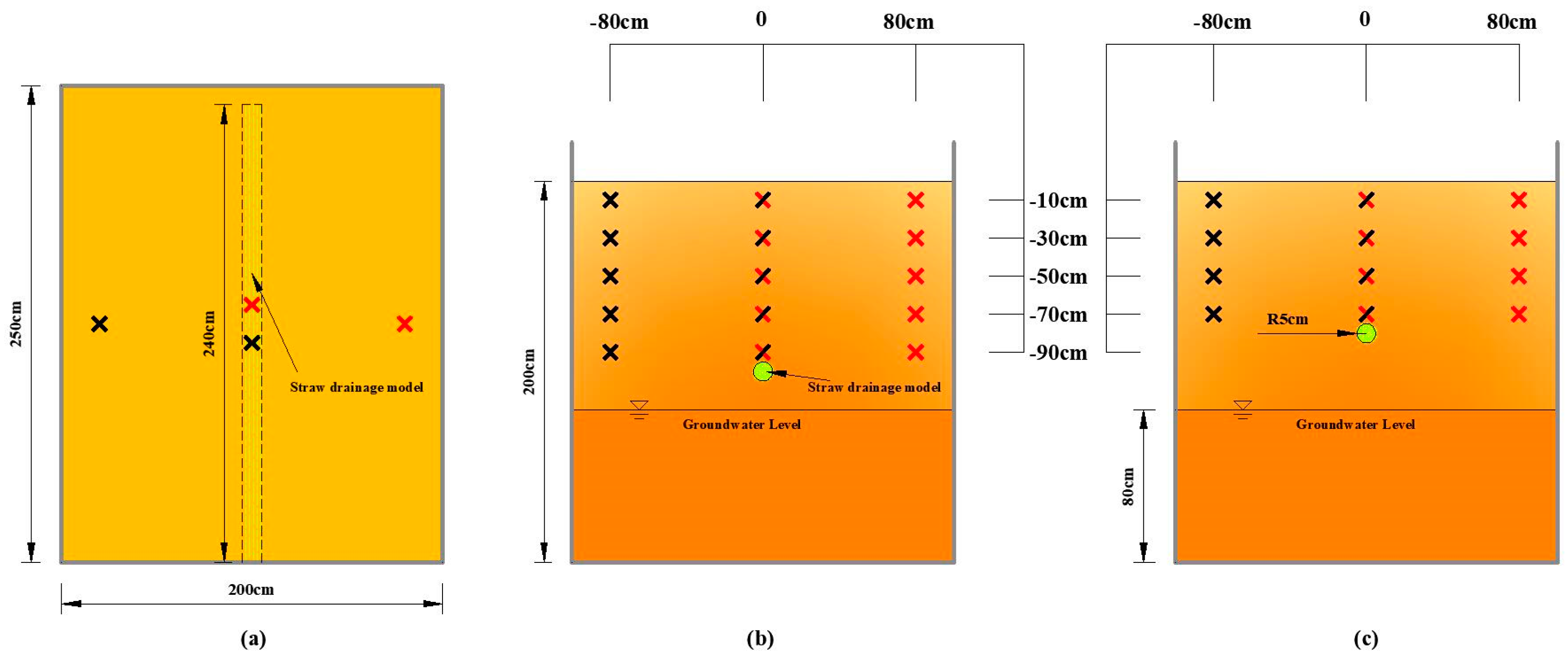
Due to the symmetry of this experimental apparatus, the half side of the vertical cross-section can adequately reflect the water-salt distribution in the whole soil profile. Thus, the soil in one side of the lysimeter was sampled for moisture measurement, and the other side of the soil was sampled for salt content testing. The sampling positions in the direction perpendicular to the drainage pipe were located horizontally at 0 and 80 cm and vertically at the soil depths of 10, 30, 50, and 70 cm for D1 treatment, and from 10 to 90 cm at a 20 cm interval for D2 treatment (Figure 1). Soil samples for testing water content and salt concentration at specific positions of the lysimeter were collected using an auger (2 cm in bore diameter and 120 cm in length) about every three days, and sampling holes were re-filled with soil in a similar property to prevent the emergence of preferential flow. The soil gravimetric water content measured by the oven drying was converted to volumetric water content by using the average observed bulk density (1.40 g cm−3). Soil salinity can be quantified in terms of the electrical conductivity of the soil water extract [18,28]. Thus, soluble salt estimates were based on extracts with a 1:5 soil:water ratio (EC1:5), determined using a DDBJ-350 EC meter (Shanghai INESA Scientific Instrument Co., Ltd., Shanghai, China). The soil-water mixture was oscillated for about 20 min and then centrifuged for testing the supernatant. The electrical conductivity of the saturated soil (ECe), which reflects the salt concentration of soil water [29], was measured using the soil samples with a wide range of EC1:5 values, and EC1:5 was converted to ECe using the relationship (R2 = 0.952) developed in laboratory:
ECe = 9.33EC1:5 + 1.25
These ECe values were then converted to the electrical conductivity that would exist in the soil solution (ECsw) using following equation [30]:
where SP is the soil saturation percentage, %; and θ is the volumetric soil water content (cm3 cm−3).
For mass balance analysis, the concentration of total dissolved salt (TDS, g L−1) in soil extract or leaching water was calculated from their EC values using the following relationship [31]:
TDS = 0.64 × EC (EC ≤ 5 dS m−1),
TDS = 0.80 × EC (EC > 5 dS m−1)
Water evaporation in the soil is the main factor for determining the soil water upper movement since there was no plant involved in this experiment and, thus, the transpiration and root water uptake were not considered at all. The soil evaporation was measured using mini-lysimeters [32] in an individual plot with the same initial condition and leaching practices. Each mini-lysimeter consisted of an undisturbed soil core contained in a plastic cylinder (12 cm diameter, 30 cm long). Additionally, another plastic cylinder, 15 cm in diameter and 30 cm long, was prepared as the sleeve to load each mini-lysimeter, and there was a holed cap at the base of each sleeve to allow for vertical water movement. Each mini-lysimeter was weighed and returned to the sleeve at the same time every day.
2.2. Model Development
2.2.1. Mathematical Model
The distributions and dynamics of soil water and salt were modeled with the computer simulation model HYDRUS-3D [19]. Assuming homogeneous and isotropic soil, the modified form of Richards’ equation applied to governing saturated water flow are described as follows [25]:
where θ is the soil volumetric water content (cm3 cm−3), t is time (d), x and y are the horizontal coordinate (cm), K(h) is the soil hydraulic conductivity (cm d−1), h is the pressure head (cm), and z (positive upward) is the vertical coordinate (cm).
The soil unsaturated hydraulic conductivity functions defined by van Genuchten [33] was adopted in HYDRUS-3D to describe the soil water retention curve:
where θr and θs denote the residual and saturated water content, respectively, Ks is the saturated hydraulic conductivity, Se is the normalized water content, α is the inverse of the air-entry value (cm−3), n is the pore-size distribution index, m = 1 − 1/n, and l is the pore-connectivity parameter. According to averaging conditions in a range of soils, l was estimated with the value of 0.5 [21].
The values of residual water content (θr) and saturated water content (θs) of the experimental soil were taken from laboratory test, while some other hydraulic parameters like empirical coefficients α and n and saturated hydraulic conductivity (Ks) was predicted based on the ROSETTA [34] neural network approach provided by HYDRUS regarding the measured data of soil bulk density and the percentages of soil particles due to there being no existing textural class for estimating the hydraulic parameters of crop straw in the HYDRUS software package. Hence, we propose a hypothesis that the SDM is regarded as a hydraulically-equivalent soil, and the initial values for straw hydraulics parameter estimation refer to Hudan and Sultan’s [35] experimental study, in which their data was obtained from a hydraulic-parameter inverse estimation of the straw interlayer. The finally-adopted hydraulic parameters of the experimental coastal soil (θr = 0.0721 cm3 cm−3, θs = 0.413 cm3 cm−3, a = 0.05 cm−1, n = 1.65, l = 0.5, and Ks = 30 cm d−1) and maize straw (θr = 0 cm3 cm−3, θs = 0.540 cm3 cm−3, a = 0.05 cm−1, n = 2.0, l = 0.5, and Ks = 1200 cm d−1) for the present modeling study were optimized during calibration. The three-dimensional non-reactive solute transport in homogeneous medium is described by the governing advection-dispersion equation [36,37]:
where θ is the volumetric water content; c is the solute concentration in liquid phase, ML−3; t is the time, T; xi, xj (i, j = 1, 2, 3) are the spatial coordinates L; qi (i = 1, 2, 3) are the water fluxes in three directions L T−1; Dij is the hydrodynamic dispersion coefficient tensor L2 T−1, which can be defined as follows [38]:
where and are the longitudinal and transverse dispersivity L; is the Kronecker delta function; is the is the absolute value of the Darcian fluid flux density, L T−1; is the molecular diffusion coefficient in free water, L2 T−1; and is the tortuosity factor.
According to many previous studies on the numerical model research of the soil salt distribution or dynamics [30,39,40], the longitudinal dispersivity was typically assumed to be one-tenth of the modeling domain along with a transverse dispersivity DT = DL/10, and the molecular diffusion coefficient in free water was set equal to 1.63 cm2 d−1 [41]. During the model testing and mass balance analysis, the EC values (dS m−1) of the leaching water and soil water extract were calculated based on Equations (1)–(4).
2.2.2. Modeling Domain and Initial and Boundary Conditions
Numerical simulations were carried out for four drainage systems with the same initial conditions, but with different burying depth or leaching water salinity. Geometries characterizing the water flow and salt transport domain set up in HYDRUS-3D modeling with each domain was discretized more than 30,000 3D-elements. Measured data of soil water and salinity were recorded on April 30, 2017, and were used as the initial condition. The flow domain was vertically divided into six layers (0–20, 20–40, 40–60, 60–80, 80–120, 120–200 cm), the water content and salt concentration of the five upper layers was set based on the corresponding values of five sampling depths (Figure 1), and the soil layer below the groundwater table (120 cm) was set as saturated. A time-dependent boundary condition, which considers the leaching water amount and soil evaporation, was imposed on the soil surface as the atmosphere boundary. Due to this experiment being conducted in large lysimeters with high-strength concrete side walls, we thus assume that no exchange of water or salt took place along the surrounding vertical sides of the modeling geometry domain (no-flow boundary) except for a seepage face (10-cm diameter circle), which represents a water outlet allowing drainage connected to the SDM. During the entire experiment, the groundwater maintaining system recorded that no water was supplied to each lysimeter. Thus, the no-flow boundary was also enforced to the bottom of the three-dimensional flow domain. Meanwhile, the third-type of solute transport boundary was used to describe the salt entering or discharging at the soil surface and drainage outlet of SDM.
Observation nodes for calibration and validation were selected in the simulation domain corresponding to those field-sampling positions (Figure 1). The model was calibrated using the data of soil water-salt content measured at the middle and side position in the D2W2 treatment, respectively, and then validated the model by comparing the simulated data with the measured average data of two positions. Additionally, to test the applicability of the hypothesis (considering crop straw as a highly-permeable soil), those configured hydraulic parameters were further applied in establishing the models of other treatments (D1W1, D1W2, and D2W1) to implement a further validation by comparing the data of soil water-salt content from the model simulation and field measurement. The calibrated and validated models were used to simulate the water movement and salt distribution in the soil profile and to estimate the mass balance of water and salt for all treatments. Additional simulations were conducted to identify the effect of leaching water quantity and quality, as well as the number of leaching events on the soil water flow and salt dynamics under the application of SDM. The design parameters of leaching practice for evaluating such effects are shown in Table 1 where the seawater mixture rate is the proportion of applied seawater per unit volume of leaching water and the number of leaching events refers to how often the equal time-interval leaching event occurred within 30 days (e.g., three times means the flow domain received three leaching events during 30 days and leaching events occurred at 10-day intervals). All of the additional model simulations were made with a drain at a depth of 1 m.
Additionally, in this context, we present two evaluation indices for quantitatively representing the desalination performance of different combinations of design parameters. One is the salt removal efficiency (SRE) determined as the ratio of the salt mass in drain water to the salt mass in the leaching water, when SRE value >1 means that the salt in the leaching water did not retain in the soil [5,30], and the next is the soil desalination rate (SDR) which is calculated as SDR = (SCB − SCE)/SCB, where SCB is the salt content at the beginning of the experiment, and SCE is the salt content at the end of the experiment. A positive value of SDR means soil desalination and a negative value means soil salinization. In this study, the SDR was calculated using the uppermost 40 cm of the soil profile, which takes the root zone of rice (Oryza sativa L.) as a reference, since rice is the most popular staple crop in Eastern China [42].
2.3. Statistical Analysis
The performance of the HYDRUS-3D model was evaluated by comparing the simulated and measured value and quantified in terms of three following statistical measures:
where the Mi and Si are the measured and simulated data, respectively, and n is the number of observations. is the mean value of the measured data. ME is the calculating the mean error; RMSE is the root mean square error, the lower the value of RMSE, the better the simulation performance of the model; the NSE is a dimensionless quality for reflecting the relative magnitude of the residual variance between the simulated and measured data, and values of NSE can vary between −∞ and 1. R2 is the coefficient of determination which was applied for testing the proportion of variance in the measured data explained by the HYDRUS model. Values of R2 range from 0 to 1, with higher values indicating less variance, and values over 0.5 considered acceptable, typically [43].
3. Result and Discussion
3.1. Model Calibration and Validation
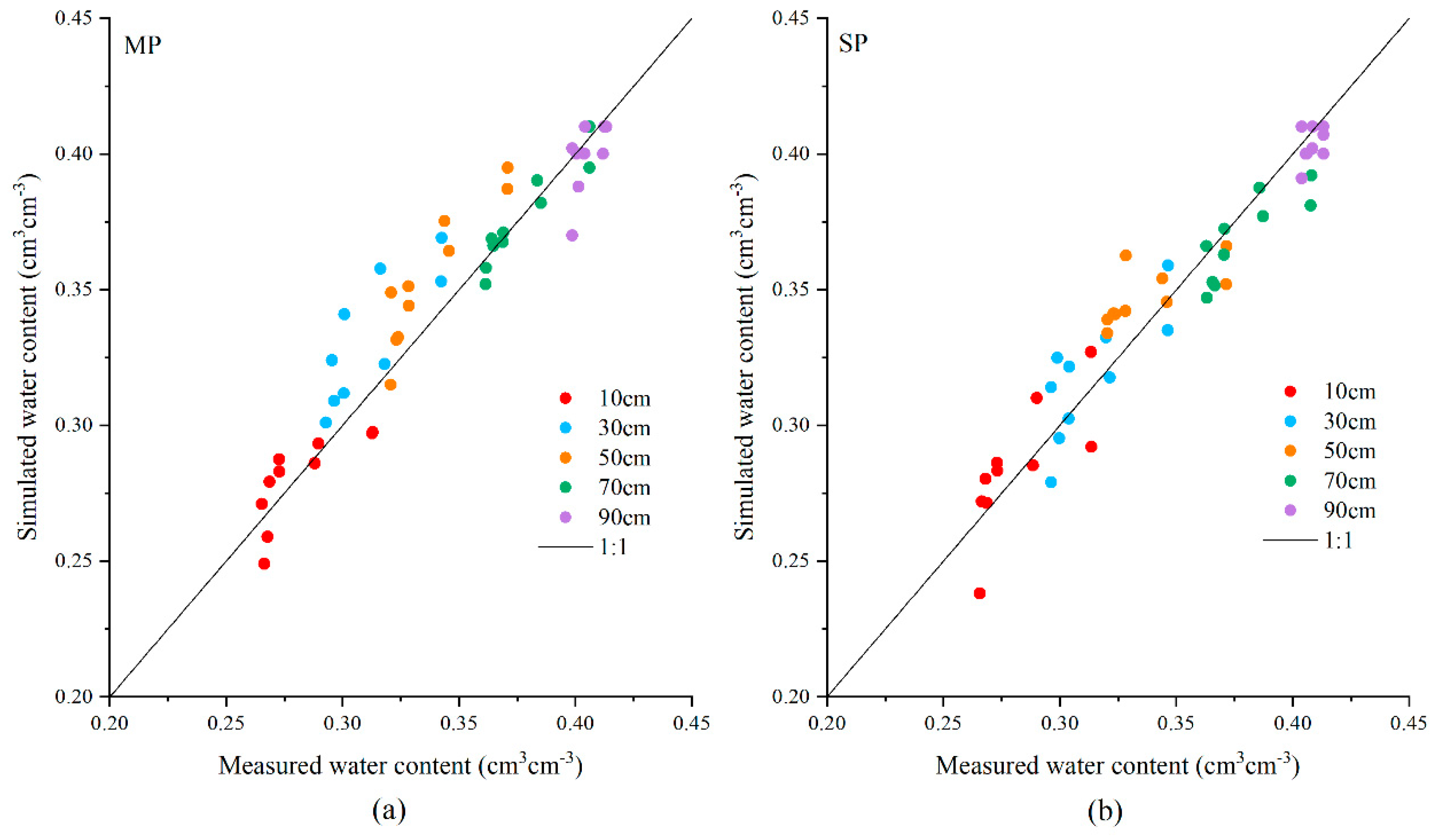
Field-measured data of soil moisture and salt content at different sampling locations in D2W2 treatment were adopted for the model calibration and validation. The calibrations were performed using the measured data at the middle and side position of the experimental lysimeter (Figure 1), respectively. The calibration of water content shows a good agreement in both positions (Figure 2), and the statistical errors parameters (RMSE, ME, NSE, and R2) values in Table 1 ranged within acceptable limits compared with similar studies [18,24]. During validation, from the model calibrated with side-position data, a positive value of ME illustrates that the model under-estimated the field-measured data of the middle position. However, the RMSE (0.018), NSE (0.799), and R2 (0.882) in the validation of the middle-position data indicated that the model still provided a good representation. Similarly, when model operated with the soil hydraulic parameters calibrated from side-position data, the statistical error parameters of RMSE (0.017), NSE (0.857), and R2 (0.877) indicated a close match between measured and simulated values at the side position. From the result of validation in soil moisture, it is reliable to optimize the value of the soil hydraulic parameters by calibrating the water content data in the middle or side sampling position.
The procedures of calibrating and validating the soil salt distribution were the same as those in the soil water content. The calibration based on either the middle position data or the side position data showed a close match between measured and simulated EC values (Figure 3 and Table 2). However, during validation, the model calibrated using the middle position data show a relatively high under-estimation (ME > 0) when simulating soil salinity for the side position. Additionally, the values of NSE (−0.073) and R2 (0.449) in the middle position data calibrated model did not perform as well as they performed in the calibrated model based on side-position data. Better performance of the soil salinity simulation from the model calibrated with side position data could be explained by the installation of the SDM, since the testing soil was filled in each lysimeter before burying the SDM, thus, the hydraulic parameters (i.e., bulk density or porosity) of the soil above the SDM (middle position) could be disturbed by the practice of excavation and backfill. Furthermore, soil evaporation during the experiment induced soil salt upward movement thereby increasing the salt accumulation in the surface soil [39], and such non-uniform distribution of salt in the soil profile could further enhance the deviations between field-measured and simulated variables during calibration and validation.
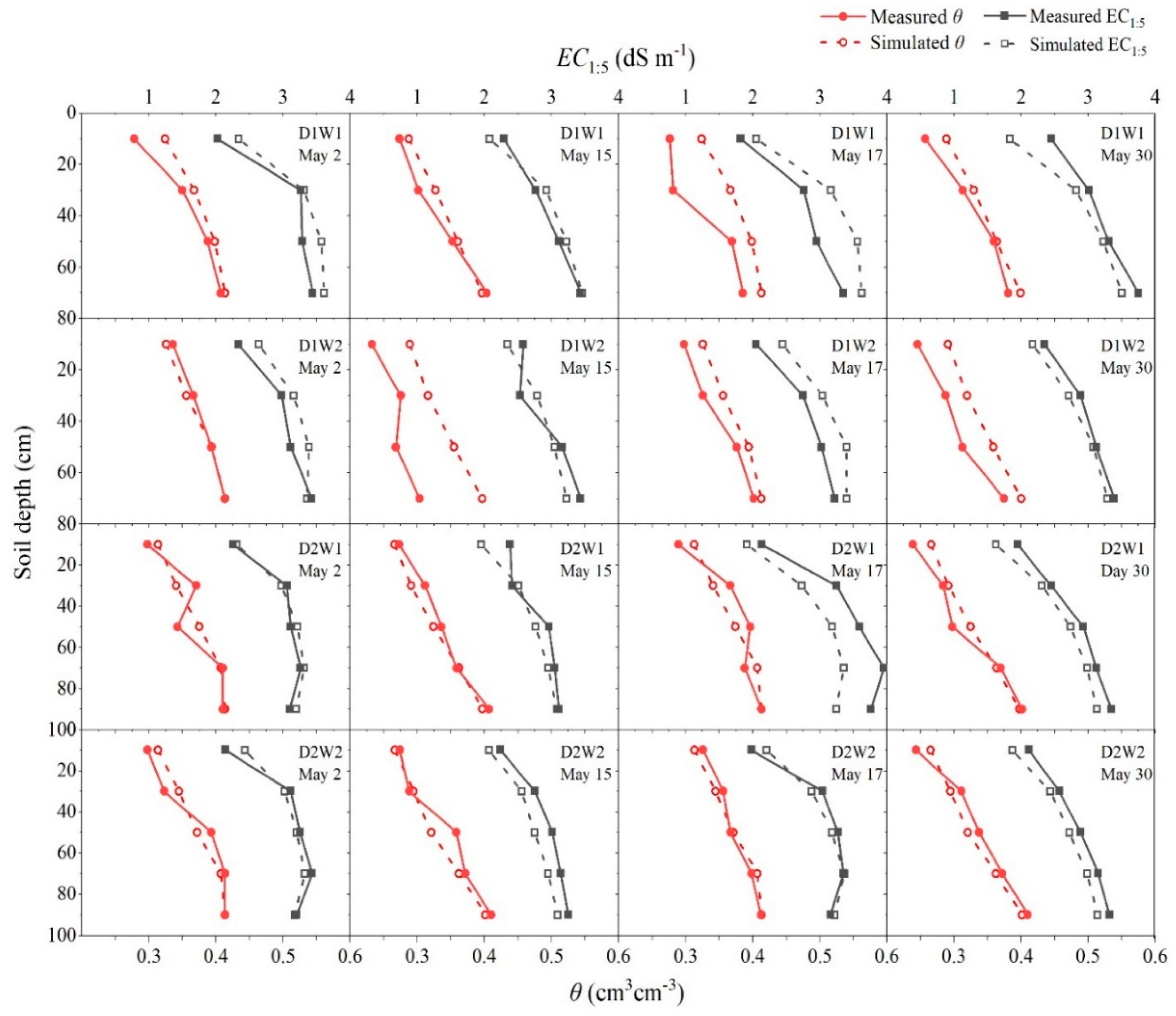
The hydraulic parameters calibrated with side position data were further applied to establish the model for simulating the water and salt content distributions in other treatments (D1W1, D1W2, and D2W1). The simulated water content distribution in different soil depth show a close correspondence with the measured values for each treatment at the indicated time (one day and 15 days after each leaching practice). From Table 3, the variation of statistical parameters indicated an acceptable simulation in the treatment of D1W1 and D1W2 despite that there was a small over-estimation of soil water content during the second leaching event (Figure 4). The increased extent of deviations during the second leaching process could be mainly attributed to the presence of the crack-preferential pathways formed by wetting-drying cycles, which accelerated the downward movement of soil water and considerably affected the water content distribution at upper soil layer [44], and such phenomenon could be intensified as the SDM is buried at a shallow depth (D1). The variation of temporal and spatial distribution of simulated soil salinity is consistent with the variation of those measured values. Despite the values of those statistical parameters fluctuated within an acceptable range [45], the values of NSE and R2 in terms of soil salt were comparatively lower than the corresponding values in the calibration and validation of soil moisture (Table 3). In this study, the calibration was just conducted with the D2 condition, some differences in model structural of D1 treatment may not be well accounted, and this could reduce the accuracy of the simulation in other treatments. Despite these numerical gaps between measured and simulated soil salt content, the deviations estimated are no higher than those reported in other studies [25,43].
3.2. Water Movement and Salt Distribution.
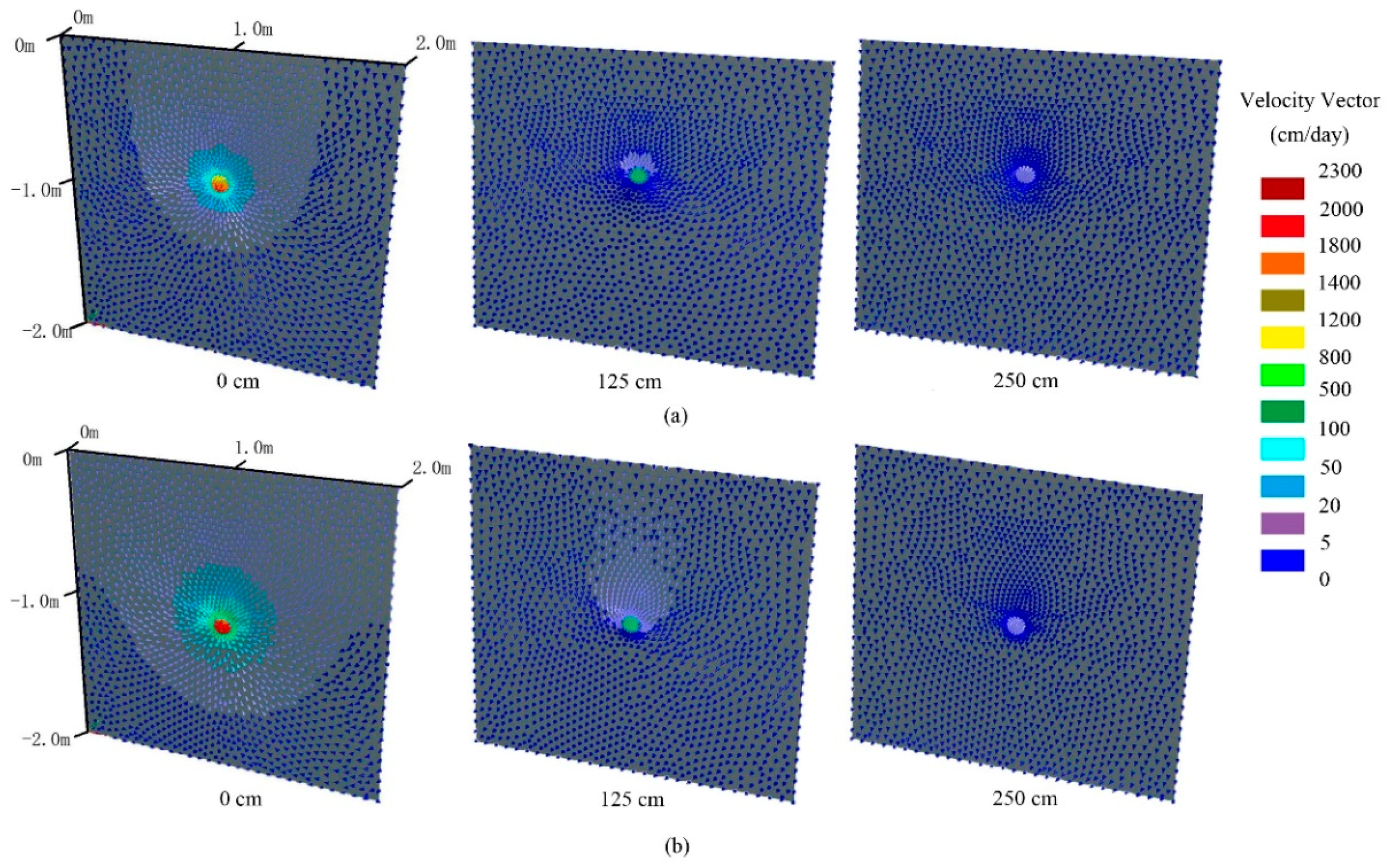
As shown in Figure 5, the intensity of velocity vectors in soil profile shows a negative relationship with the distance between soil profile and drain outlet. In the SDM leaching system, the seepage face was only set on the vertical boundary of the outlet (Figure 1), and this outlet was also the interface between SDM and outside air. Thus, the horizontal movement of soil water in the SDM could be the synergistic effect of pressure head combined with the high permeability of maize straw, and meanwhile the influence of pressure head on water flow mainly concentrated on the seepage face boundary which, in turn, caused a gradual decrease of the soil water velocity with the increase in the distance between the soil profile and the drain outlet. Such a phenomenon is different from those conventional subsurface pipe drainages, in which the movement of water is in the same pattern among all the vertical soil profiles perpendicular to the drain pipe [46,47], but the similarity among those two systems is that the deeper drain treatment could affect a broader range of soil moisture movement than the shallow one.
Figure 5 also depicts the streamline patterns of soil water movement. The overall tendency of streamlines show a concentration towards the location of the SDM, and soil water near the left and right boundary firstly move vertically and then converge towards the SDM. During the leaching process, leaching water at the side position of the soil profile initially infiltrated vertical and then tangentially flowed to the SDM, hence they need to take a longer time to arrive at the SDM compared to the infiltration at the middle position where the streamline pathway is short and straight which, in turn, reduced the loss of gravitational potential energy of the infiltration water, and ultimately increases the velocity of soil water movement. The streamline of the simulated water movement is consistent with those of subsurface drains, which is experimentally observed by Mirjat, et al. [48] and modeling proved by Mirjat, et al. [47].
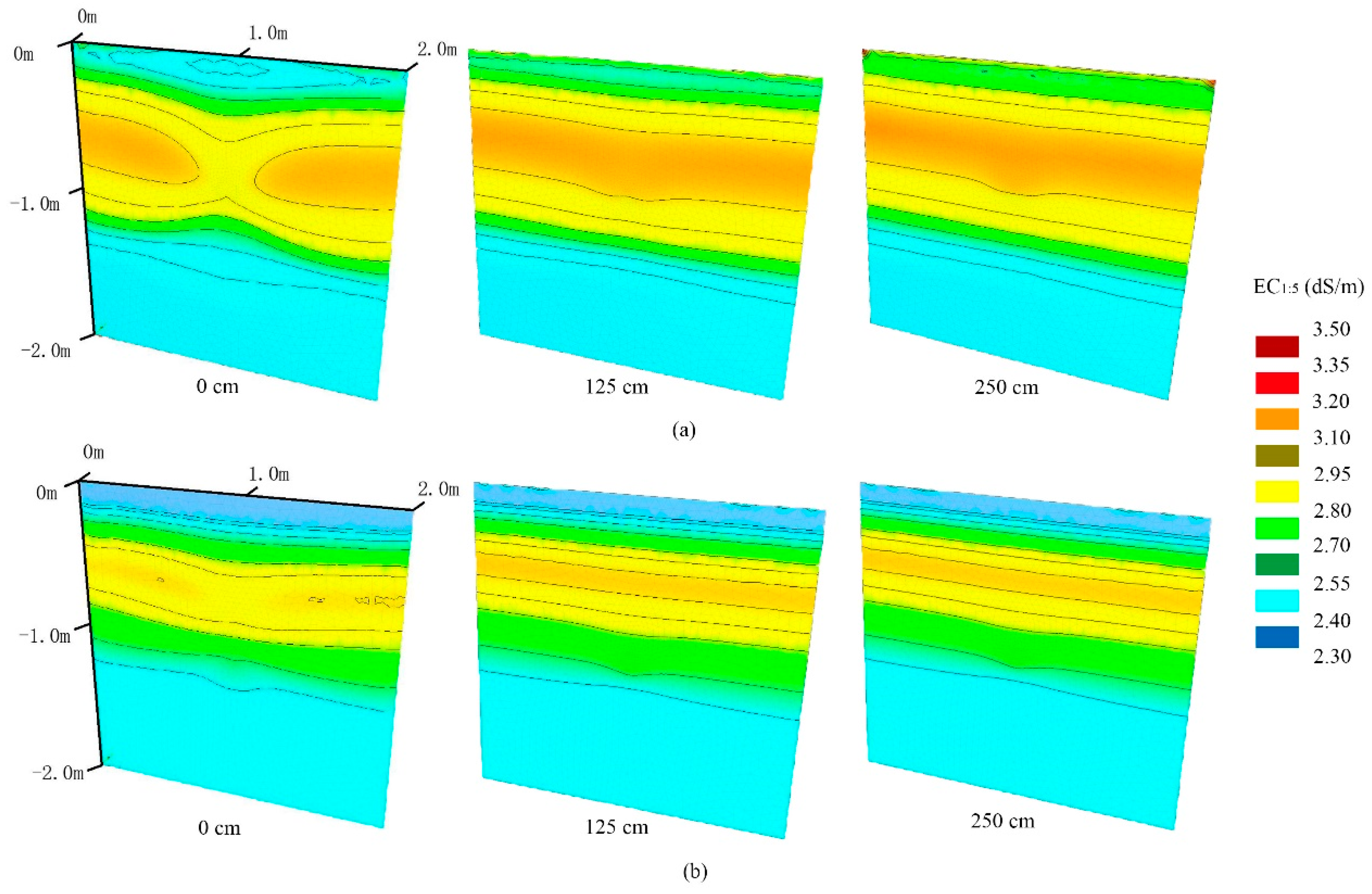
As the salt distribution pattern suggested by Figure 6, there is an obvious desalination zone formed within about 0.0–0.3 m of the soil layer in both two treatments, despite a relatively higher salt content within 0.3–1.0 m. The size of the high salt layer was narrowed in the D2W1 treatment compared with D1W1, and this could be possibly attributed to the deeper burying of SDM in D2W1 in which leaching water passed through more soil layers above the SDM and eventually washed out more salt from the soil profile. Furthermore, the size of the desalination zone was not uniformly layered at the soil profile of the outlet, especially in the D1 treatment. Such nonuniformity in the salt distribution can be observed closely resembling the above-mentioned water movement pattern since the diffusion and accumulation of soil salinity are accompanied with the physical processes of moisture transfer. The straight and short streamline of water infiltration at middle position enhanced the leaching efficiency, which formed a desalination region below and above the SDM. In contrast, the circuitous and long streamline of side-position infiltration limited the transport of the solute in the soil profile and then caused salt accumulation on both sides of the SDM, finally forming a butterfly shape of the salt distribution.
3.3. Mass Balance of Soil Water and Salt
From Table 4, the simulated water balance indicated that water drained in first leaching event was varied from 60.7 to 105.6 mm (D2W1 > D2W2 > D1W1 > D1W2), which accounts for 37.9–66.0% of the total amount of the water input for leaching. During the second leaching event, although the soil evaporation was slightly higher, the drainage amount was increased compared to the first event for all treatments, especially in shallow drain depth condition (D1) which show an approximate 10% increase. The increased drainage amount in the second leaching event was ascribed to the soil water content increasing by the first leaching event, and treatments at a shallow drainage depth could further increase the drainage amount for the subsequent leaching events. The total water outflow in treatment with high leaching water salinity (W2) was decreased by 0.9% in the D2 condition but increased by 1.1% in the D1 condition, respectively, as compared to the corresponding values in treatments leached with low-salinity water (W1). This indicated that the total drainage discharge may not have an explicit relationship with the salinity of the leaching water.
For the mass balance of salt, the averaged quantity of salt removed from these four treatments was about 1.7 times of the salt input from the diluted seawater. Additionally, the negative value of soil salt storage indicated that there is no salt build-up in the soil profile (0–120 cm), and the positive value only existed in the D1W2 treatment, which means using the SDM system for soil desalination is feasible with an increase in the drain depth or reduction in the salinity of the leaching water. This result is in accordance with previous studies about conventional subsurface drainage [49,50] in which increased drain depth ensured more soil layers were leached and, thus, raised the salinity of the discharge. Additionally, the average amount of salt removal of all treatments in the first leaching event was about 6.7% higher than that of the second leaching event, suggesting that the effect of antecedent leaching events on salt transport could influence the mass of salt removal in subsequent leaching events [50,51].
3.4. Evaluation of the Leaching Capacity of Straw Drainage Modules
3.4.1. Cumulative Outflow and Salt Removal
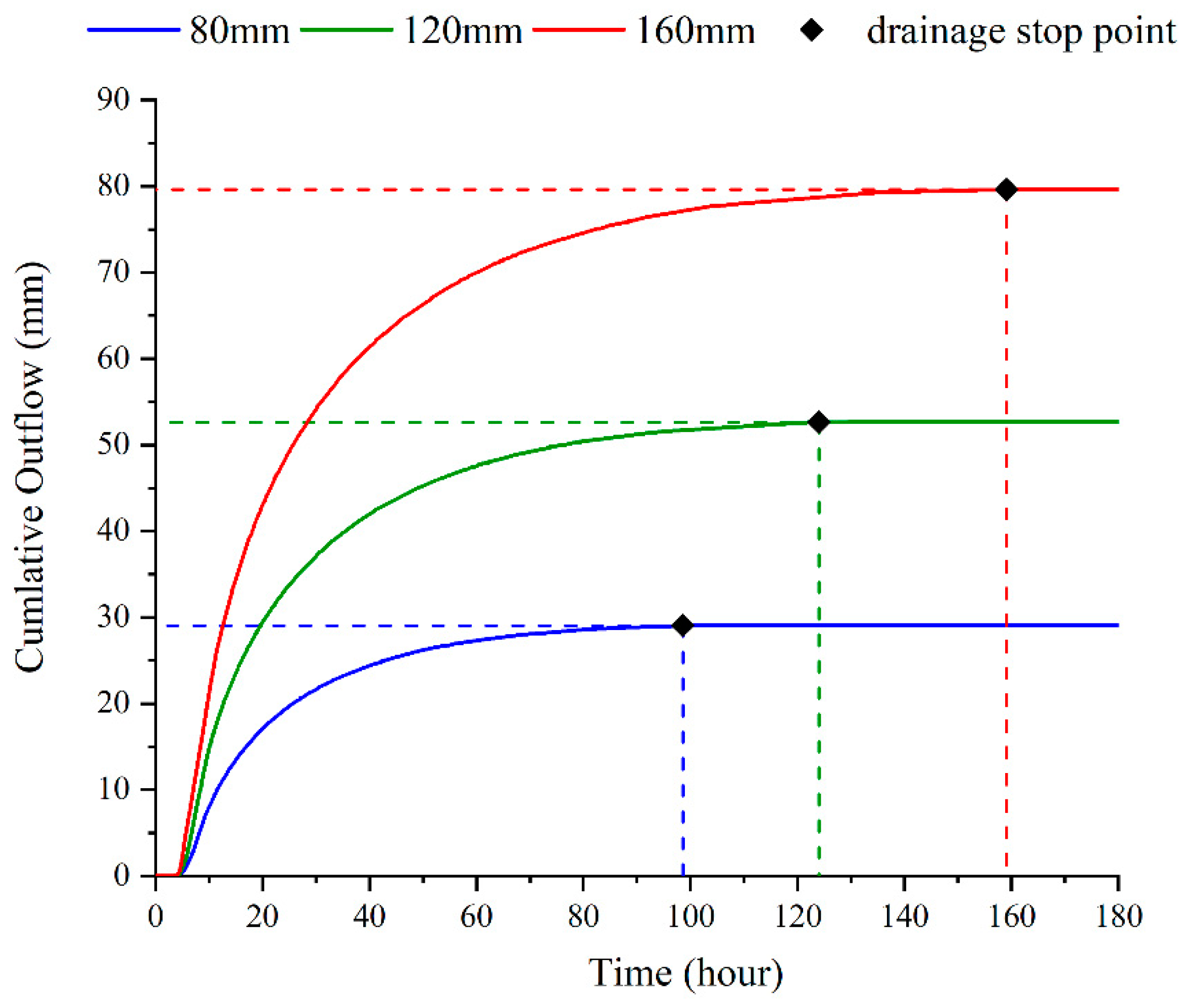
From the simulation of cumulative outflow, when leached with the same water amount, the coinciding cumulative-outflow curves were found in treatments with different salt levels of leaching water, which suggests that the cumulative outflow and drainage duration (i.e., the duration of time from when the drainage system starts draining to when the cumulative outflow no longer increased) has no relevance to the salinity of the leaching water. This result could be accepted because the EC value of the leaching water or the percolating solution in this study were exceeded 5.6 dS m−1 and the sodium absorption ratio (SAR) was beyond 20, soil water under this condition has a low probability to induce the infiltration problem of the experimental soil [52].
Furthermore, as shown in Figure 7, after rapid growth and then successive slow growth of cumulative outflow, the treatments with leaching amount of 80, 120, and 160 mm spent 99, 123, and 159 h to reach their stabilized maximum of cumulative outflow (29, 53, and 79 mm), respectively. Similar result was generally proven by previous studies on subsurface drainage system design [11,53,54], in which the leaching water amount is positively associated with the drainage discharge but negatively related to the drainage duration. Moreover, a large amount of saline leaching or irrigation water can degrade the soil structural stability over time, thereby reducing the soil permeability and infiltration rate [55] which, in turn, causes a variation in soil hydraulic parameters. This cumulative effect was not considered during the modeling testing since the duration of our field experiment was just 30 days. Therefore, the situation of soil degradation needs to be further studied through long-term experiments.
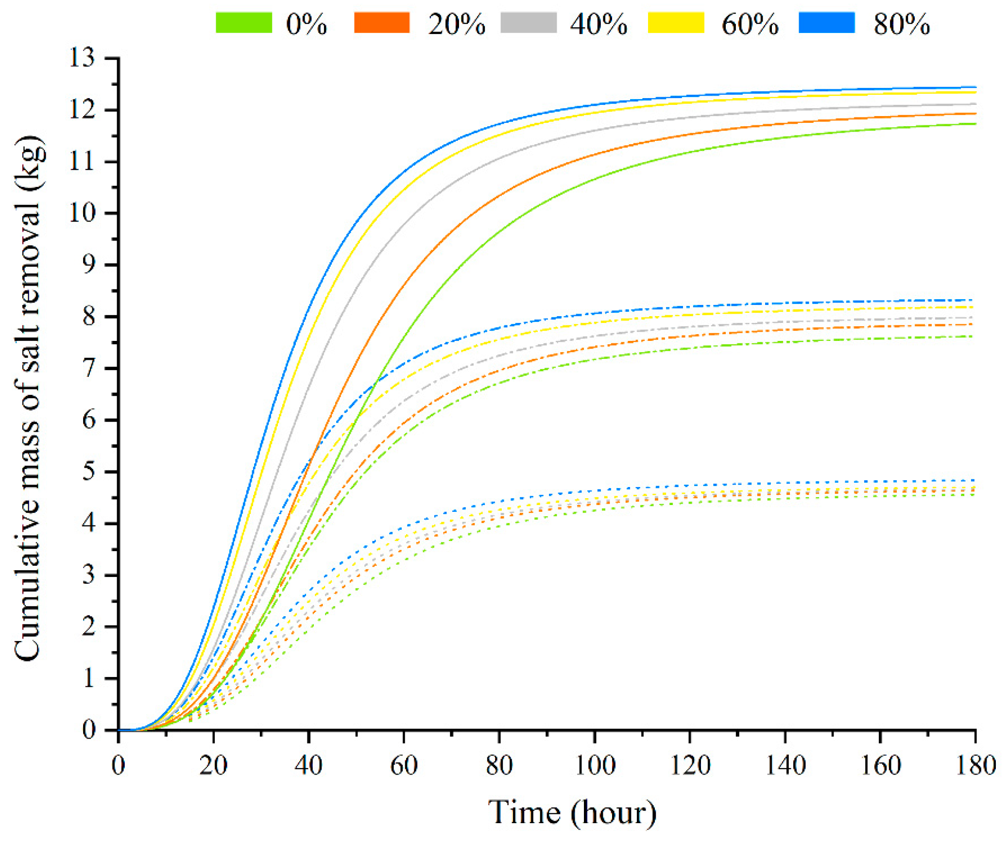
From the simulation results in Figure 8, the increased total mass of salt removal was obtained in treatments with a high amount or high salinity of leaching water, but the difference of the cumulative mass of salt removal between treatments with different leaching water salinity was gradually narrowed with time. Since the outlet is the only seepage face in the SDM leaching system, the time for soil water discharge might be longer as compared to those conventional subsurface drainage systems, where the inner wall of drain pipes or tubes were all equal to the seepage face boundary [24]. However, the extended period of drainage duration is favorable for adequately dissolving soil salt and finally improving the effect of leaching water salinity on salt removal. On the contrary, those conventional subsurface drainage systems promoted the drainage rate in the soil profile but shortened the dissolving time for soil leaching, which made the drainage performance sensitive to the quality of the leaching water.
3.4.2. Variation of Soil Salt Content
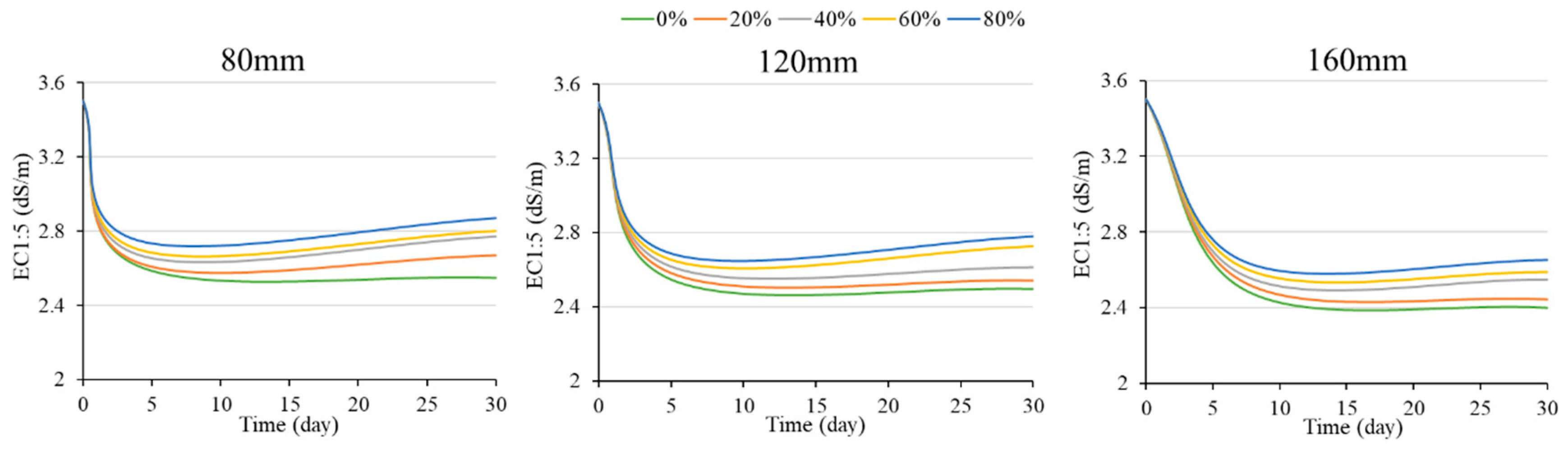
Simulation of the salt content within the average root zone during an individual leaching event is presented in Figure 9. In all cases, a sudden drop of soil salt in the average root zone (0–40 cm) was obtained during 0–3 days. After that, salt content increased again due to the upward water movement by soil evaporation. However, this kind of secondary salinization becomes less pronounced with the reduction in the salt level of the leaching water or the increase in the leaching water amount, since no rebound of EC values was found in the 120 mm and 160 mm treatments when the mixture rate is lower than 20%. Notably, the discrepancy in root zone salt content among five leaching water qualities was narrowed by increasing the leaching water amount, since the EC values ranged from 2.55 to 2.87 dS m−1 for 80 mm treatments and 2.40 to 2.56 dS m−1 for 160 mm treatments at the end of the experiment. The narrowed gap of soil salinity rebound in high leaching amount treatments could be explained by the increase in the amount of leaching water reducing the soil salt content which, in turn, decreased the degree of soil salt upward movement.
3.4.3. Desalination Performance
As suggested in Figure 10, during an individual leaching practice, a dramatic drop of SRE was observed when mixture rates of leaching water ranged from 0–20%, followed by a relatively steady downtrend as the mixture rates increased from 20% to 80%. Meanwhile, when leaching water at the same mixture rate, the average values of SDR were raised with the increase of leaching water amounts, which means the per unit volume of leaching water could dissolve more soil salt as the amount of leaching water was increased. The downtrend of SRE is satisfied to be fitted by exponential decay function (Figure 10) which is suitable for describing a curve that the decline rate decreased as the independent variable gradually increase. From the fitting results, the maximum acceptable (SRE = 1) seawater mixture rate for leaching amount at 80, 120, and 160 mm was calculated as 37.27, 44.95, and 52.57%, respectively, which means the salt in the leaching water would not remain in the soil profile as the seawater proportion of leaching water were lower than such percentages.
On the other hand, the positive values of SDR were obtained in all treatments, suggesting the salt content within the root zone were reduced compared with the initial condition. Similar to the variation of SRE the values of SDR were also raised with the increase of leaching water amount, and the linear-regression was adopted to analyze the relationship between SDR and mixture rate of leaching water. As suggested in Figure 10, SDR values decreased by 5.2, 4.2, and 2.5% for every 1% increase of the mixture rate as the leaching water amount was applied at 80, 120, and 160 mm, respectively, which means that the SDR was more sensitive to leaching water salinity under lower water application amounts. That is to say, in the SDM leaching system, reducing the salinity of the leaching water could be more helpful to achieve better soil desalination when the amount of leaching water is small.
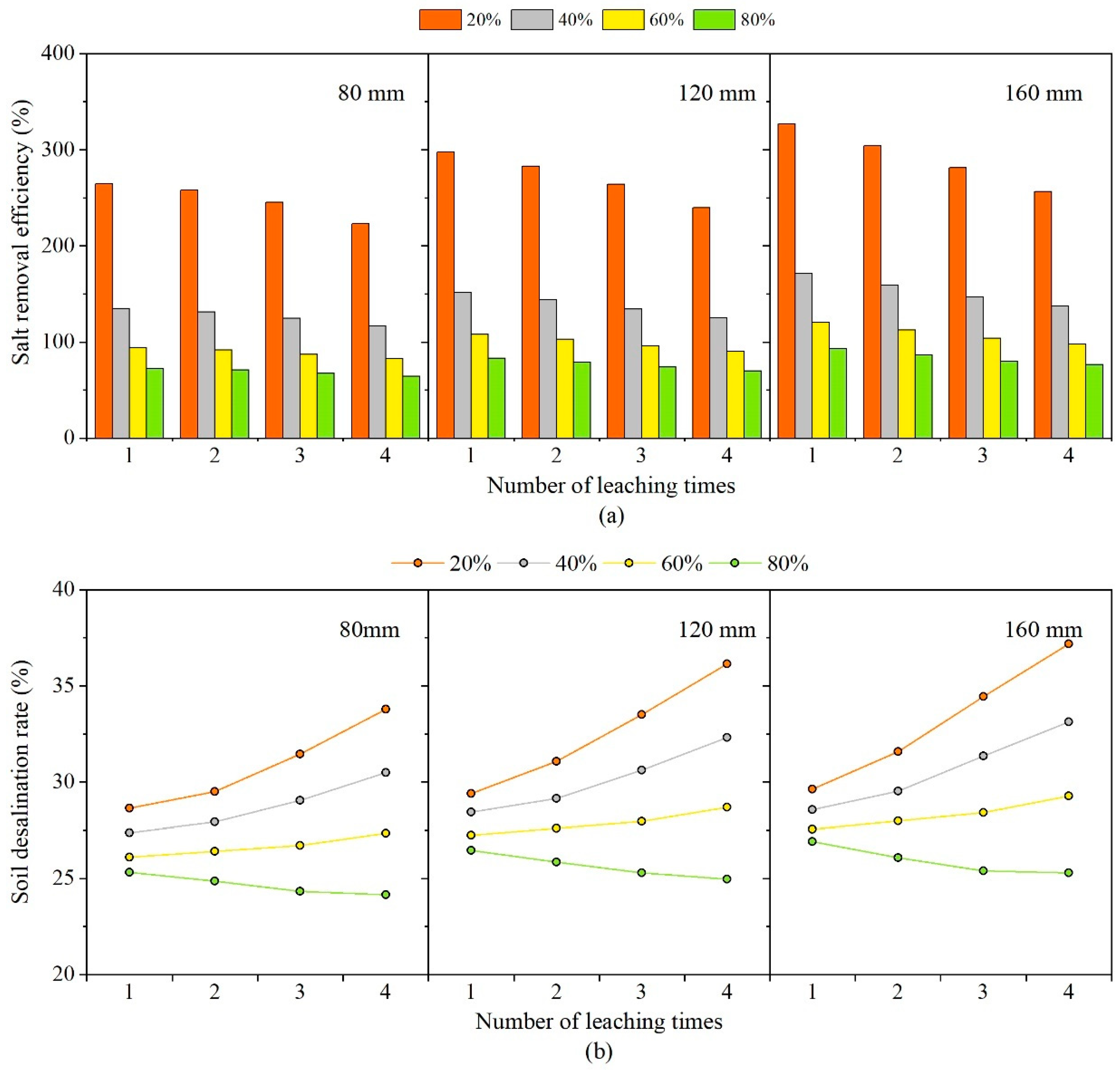
Since the difference of salt transport was present between the first and second leaching events (Section 3.3), we further explored the effect of leaching water salinity and the amount on desalination performance of the SDM when adding to the number of leaching events (Figure 11). As suggested in Figure 11a, under the same amount of leaching water, the value of SRE was reduced with the increasing number of leaching events, and the degree of such a decrease was enhanced in treatments leached with low-salinity water, since the average values of SRE among three leaching amounts were decreased about 17.35% and 15.02% for each additional leaching event at the mixture rate of 20% and 40%, respectively, while the corresponding values were dropped to 11.83% and 10.99% when the mixture rate arrived at 60% and 80%, respectively. This was ascribed to the salt content being reduced by antecedent leaching events and, hence, those subsequent events with the same leaching amount could not remove more salt from the soil profile, especially in those low-salinity water leaching treatments which bring out more salt during antecedent leaching events. Similar results were obtained by Wang, et al. [56], who reported that the desalination performance could not be maintained at a high level with the continuous increase in leaching events.
On the other hand, when the salinity of leaching water is in a relatively low level, increasing the number of leaching events could achieve a high soil desalination rate even the total amount of leaching water was the same (Figure 11b). For example, the SDR value in two times leaching with 160 mm was lower than the SDR value in four leaching events with 80 mm if the mixture rate was lower than 60%. Figure 11 also reveals that the favorable impact of low-salinity leaching water for removing soil salt and the negative impact of high-salinity leaching water for salt build-up in the soil were both intensified by increasing the number of leaching events, since the highest and lowest SDR values were both observed after four leaching events in treatments leached with seawater at a mixture rate of 20% and 80%, respectively.
4. Conclusion
In this study, to examine the potential of straw drainage module (SDM) as a temporary subsurface drainage facility under leaching with diluted seawater in initial reclamation of coastal saline soil, a three-dimensional mathematical model (HYDRUS-3D) was developed to simulate soil water flow and salt transport under the application of SDM. The measured data of soil moisture and salinity from the field experiments in large lysimeters was used to calibrate and validate our model. The model performed reliably in representing the distributions of soil water content and salt concentrations when the SDM was included in the model as a tube of highly permeable soil.
Simulation results of the dynamic pattern and the mass balance of soil water and salt revealed that the soil water velocity and salt distribution in the soil profile were both affected by the drain outlet, and such an effect was enhanced as the soil profile approaching the drain outlet. An increase in the drain depth of the SDM or reduction in the seawater proportion in the leaching water could help drive more salt out of the soil. Additionally, despite the inter-treatment differences in the SDM drain depth and leaching water quality, the drainage discharge and salt removal amount are primarily dependent on the antecedent content of soil water and salt.
The HYDRUS-3D model was further applied to explore the impacts of design parameters of the leaching amount, seawater proportion in the leaching water, numbers of leaching events, and their relationship with the performance in terms of soil desalination. The result of the simulation showed the effect of leaching amount and leaching water salinity almost met the same rules as that in conventional subsurface drainage except for the cumulative mass of salt removal. During an individual leaching event, the SRE and SDR were both positively correlated to the leaching water amount and negatively correlated to the leaching water salinity, and for preventing the salt buildup in the soil profile the threshold values of the mixture rate are 37.27, 44.95, and 52.57% when the leaching amounts are 80, 120, and 160 mm, respectively. Adding the number of leaching events could enhance the soil desalination when leached with low salinity water but could also aggravate the salt retention from high-salinity leaching water, and such effects could be further pronounced if there is an increase in the amount of leaching water. Therefore, as the seawater is diluted to a suitable percentage, a lesser leaching amount combined with frequent leaching events or a large leaching amount with fewer leaching times are suggested in the SDM leaching system design.
Overall, under reasonable design parameters, the utilization of diluted seawater is an alternative method in alleviating the scarcity of freshwater resources, and the eco-friendly and low-cost straw drainage module demonstrates similar performance in terms of soil water and salt control as that in a conventional subsurface drainage system. Thus, the SDM leaching system could be a good option to address the problem of soil salination in the short-term and avoid high construction costs for the initial reclamation of coastal soil. It is recommended that additional studies and cost-benefit assessments be conducted at specific sites under specific hydrological and salinity conditions.
Author Contributions
P.L. and Z.Z. (Zhanyu Zhang) designed this study. P.L., M.H., and Z.Z. (Zemin Zhang) contributed to field experiment and data processing. P.L. and Z.S. developed and operated the HYDRUS-3D model. P.L. prepared the original Draft. Z.S. and Z.Z. (Zhanyu Zhang) reviewed and edited the manuscript.
Funding
Funding for this research was partially supported by the Natural Science Foundation of China (no. 51579069), the Fundamental Research Funds for the Central Universities (2017B691X14), the Scientific Research Innovation Projects in Jiangsu general Universities (KYCX17-0437), and the USDA-NIFA Hatch Project (grant no. TEX0-1-9448).
Conflicts of Interest
The authors declare no conflict of interest.
References
- Wang, F.; Wall, G. Mudflat development in Jiangsu Province, China: Practices and experiences. Ocean Coast. Manag. 2010, 53, 691–699. [Google Scholar] [CrossRef]
- Long, X.H.; Liu, L.P.; Shao, T.Y.; Shao, H.B.; Liu, Z.P. Developing and sustainably utilize the coastal mudflat areas in China. Sci. Total Environ. 2016, 569, 1077–1086. [Google Scholar] [CrossRef] [PubMed] [Green Version]
- Wang, S.; Qu, X. Dynamic control of drainage and calculation method of drainage spacing based on the idea of combining the control of salinization with subsurface waterlogging. J. Hydraul. Eng. 2008, 11, 1204–1210. (In Chinese) [Google Scholar]
- Shao, X.H.; Chang, T.T.; Cai, F.; Wang, Z.Y.; Huang, M.Y. Effects of subsurface drainage design on soil desalination in coastal resort of China. J. Food Agric. Environ. 2012, 10, 935–938. [Google Scholar]
- Qadir, M.; Ghafoor, A.; Murtaza, G. Amelioration strategies for saline soils: A review. Land Degrad. Dev. 2000, 11, 501–521. [Google Scholar] [CrossRef]
- Pereira, C.S.; Lopes, I.; Abrantes, I.; Sousa, J.P.; Chelinho, S. Salinization effects on coastal ecosystems: A terrestrial model ecosystem approach. Philos. Trans. R. Soc. Lond. Ser. B Biol. Sci. 2019, 374. [Google Scholar] [CrossRef]
- Martínez-Alvarez, V.; González-Ortega, M.J.; Martin-Gorriz, B.; Soto-García, M.; Maestre-Valero, J.F. Seawater desalination for crop irrigation—Current status and perspectives. In Emerging Technologies for Sustainable Desalination Handbook; Elsevier: Amsterdam, The Netherlands, 2018; pp. 461–492. [Google Scholar]
- Guo, S.H.; Liu, Z.L.; Li, Q.S.; Yang, P.; Wang, L.L.; He, B.Y.; Xu, Z.M.; Ye, J.S.; Zeng, E.Y. Leaching heavy metals from the surface soil of reclaimed tidal flat by alternating seawater inundation and air drying. Chemosphere 2016, 157, 262–270. [Google Scholar] [CrossRef]
- Hu, Y.H.; Lindo-Atichati, D. Experimental equations of seawater salinity and desalination capacity to assess seawater irrigation. Sci. Total Environ. 2019, 651, 807–812. [Google Scholar] [CrossRef]
- Hornbuckle, J.W.; Christen, E.W.; Faulkner, R.D. Analytical Solution for Drainflows from Bilevel Multiple-Drain Subsurface Drainage Systems. J. Irrig. Drain. Eng. 2012, 138, 642–650. [Google Scholar] [CrossRef]
- Christen, E.; Skehan, D. Design and management of subsurface horizontal drainage to reduce salt loads. J. Irrig. Drain. Eng. 2001, 127, 148–155. [Google Scholar] [CrossRef]
- Bahceci, I.; Dinc, N.; Tari, A.F.; Agar, A.I.; Sonmez, B. Water and salt balance studies, using SaltMod, to improve subsurface drainage design in the Konya-Cumra Plain, Turkey. Agric. Water Manag. 2006, 85, 261–271. [Google Scholar] [CrossRef]
- Luo, W.; Sands, G.R.; Youssef, M.; Strock, J.S.; Song, I.; Canelon, D. Modeling the impact of alternative drainage practices in the northern Corn-belt with DRAINMOD-NII. Agric. Water Manag. 2010, 97, 389–398. [Google Scholar] [CrossRef]
- Lu, P.; Zhang, Z.; Feng, G.; Wan, C.; Shi, X. Effect of straw draining piece depth in soil on soil water-salt distribution in saline soil and its drainage-salt inhibiting performance. Trans. CSAE 2017, 33, 115–121. (In Chinese) [Google Scholar]
- Lu, P.R.; Zhang, Z.Y.; Feng, G.X.; Huang, M.Y.; Shi, X.F. Experimental Study on the Potential Use of Bundled Crop Straws as Subsurface Drainage Material in the Newly Reclaimed Coastal Land in Eastern China. Water 2018, 10, 31. [Google Scholar] [CrossRef]
- Montagne, D.; Cornu, S.; Le Forestier, L.; Cousin, I. Soil Drainage as an Active Agent of Recent Soil Evolution: A Review. Pedosphere 2009, 19, 1–13. [Google Scholar] [CrossRef] [Green Version]
- Allen, D.; Arthur, S.; Haynes, H.; Wallis, G.S.; Wallerstein, N. Influences and drivers of woody debris movement in urban watercourses. Sci. China Technol. Sci. 2014, 57, 1512–1521. [Google Scholar] [CrossRef] [Green Version]
- Siyal, A.A.; van Genuchten, M.T.; Skaggs, T.H. Solute transport in a loamy soil under subsurface porous clay pipe irrigation. Agric. Water Manag. 2013, 121, 73–80. [Google Scholar] [CrossRef]
- Šimůnek, J.; Van Genuchten, M.T.; Šejna, M. The HYDRUS Software Package for Simulating the Two- and Three-Dimensional Movement of Water, Heat, and Multiple Solutes in Variably-Saturated Porous Media; PC-Progress: Prague, Czech Republic, 2018. [Google Scholar]
- Boivin, A.; Simunek, J.; Schiavon, M.; van Genuchten, M.T. Comparison of pesticide transport processes in three tile-drained field soils using HYDRUS-2D. Vadose Zone J. 2006, 5, 838–849. [Google Scholar] [CrossRef]
- Ebrahimian, H.; Noory, H. Modeling paddy field subsurface drainage using HYDRUS-2D. Paddy Water Environ. 2015, 13, 477–485. [Google Scholar] [CrossRef]
- De Vos, J.A.; Raats, P.A.C.; Feddes, R.A. Chloride transport in a recently reclaimed Dutch polder. J. Hydrol. 2002, 257, 59–77. [Google Scholar] [CrossRef]
- Tao, Y.; Wang, S.; Xu, D.; Yuan, H.; Chen, H.J.A.W.M. Field and numerical experiment of an improved subsurface drainage system in Huaibei plain. Agric. Water Manag. 2017, 194, 24–32. [Google Scholar] [CrossRef]
- Filipovic, V.; Mallmann, F.J.K.; Coquet, Y.; Simunek, J. Numerical simulation of water flow in tile and mole drainage systems. Agric. Water Manag. 2014, 146, 105–114. [Google Scholar] [CrossRef] [Green Version]
- Li, S.H.; Zhou, D.M.; Luan, Z.Q.; Pan, Y.; Jiao, C.C. Quantitative simulation on soil moisture contents of two typical vegetation communities in Sanjiang Plain, China. Chin. Geogr. Sci. 2011, 21, 723–733. [Google Scholar] [CrossRef]
- Honari, M.; Ashrafzadeh, A.; Khaledian, M.; Vazifedoust, M.; Mailhol, J.C. Comparison of HYDRUS-3D Soil Moisture Simulations of Subsurface Drip Irrigation with Experimental Observations in the South of France. J. Irrig. Drain. Eng. 2017, 143. [Google Scholar] [CrossRef]
- Liu, G.; Yang, J.; Jiang, Y. Salinity characters of soils and groundwater in typical coastal area in Jiangsu Province. Soils 2005, 37, 163–168. (In Chinese) [Google Scholar]
- Chen, L.J.; Feng, Q.; Li, F.R.; Li, C.S. A bidirectional model for simulating soil water flow and salt transport under mulched drip irrigation with saline water. Agric. Water Manag. 2014, 146, 24–33. [Google Scholar] [CrossRef]
- Slavich, P.; Petterson, G. Estimating the electrical conductivity of saturated paste extracts from 1: 5 soil, water suspensions and texture. Soil Res. 1993, 31, 73–81. [Google Scholar] [CrossRef]
- Hanson, B.; Hopmans, J.W.; Simunek, J. Leaching with subsurface drip irrigation under saline, shallow groundwater conditions. Vadose Zone J. 2008, 7, 810–818. [Google Scholar] [CrossRef]
- Grattan, S. Irrigation Water Salinity and Crop Production; UCANR Publications: Oakland, CA, USA, 2002; Volume 9. [Google Scholar]
- Eberbach, P.; Humphreys, E.; Kukal, S. The effect of rice straw mulch on evapotranspiration, transpiration and soil evaporation of irrigated wheat in Punjab, India. Agric. Water Manag. 2011, 98, 1847–1855. [Google Scholar]
- Vangenuchten, M.T. A closed form equation for predicting the hydraulic conductivity of unsaturated soils. Soil Sci. Soc. Am. J. 1980, 44, 892–898. [Google Scholar] [CrossRef]
- Schaap, M.G.; Leij, F.J.; van Genuchten, M.T. ROSETTA: A computer program for estimating soil hydraulic parameters with hierarchical pedotransfer functions. J. Hydrol. 2001, 251, 163–176. [Google Scholar] [CrossRef]
- Hudan, T.; Sultan. Inverse Estimation for Soil and Straw Hydraulic Parameters from Lysimeters. J. Irrig. Drain. 2009, 28, 68–70. (In Chinese) [Google Scholar]
- Phogat, V.; Mahadevan, M.; Skewes, M.; Cox, J.W. Modelling soil water and salt dynamics under pulsed and continuous surface drip irrigation of almond and implications of system design. Irrig. Sci. 2012, 30, 315–333. [Google Scholar] [CrossRef]
- Zhu, Y.; Shi, L.S.; Yang, J.Z.; Wu, J.W.; Mao, D.Q. Coupling methodology and application of a fully integrated model for contaminant transport in the subsurface system. J. Hydrol. 2013, 501, 56–72. [Google Scholar] [CrossRef]
- Bear, J. Dynamics of Fluids in Porous Media; Courier Corporation: Washington, DC, USA, 2013. [Google Scholar]
- Phogat, V.; Pitt, T.; Cox, J.W.; Simunek, J.; Skewes, M.A. Soil water and salinity dynamics under sprinkler irrigated almond exposed to a varied salinity stress at different growth stages. Agric. Water Manag. 2018, 201, 70–82. [Google Scholar] [CrossRef] [Green Version]
- Wang, J.; Huang, Y.; Long, H.; Hou, S.; Xing, A.; Sun, Z. Simulations of water movement and solute transport through different soil texture configurations under negative-pressure irrigation. Hydrol. Process. 2017, 31, 2599–2612. [Google Scholar] [CrossRef]
- Cote, C.M.; Bristow, K.L.; Charlesworth, P.B.; Cook, F.J.; Thorburn, P.J. Analysis of soil wetting and solute transport in subsurface trickle irrigation. Irrig. Sci. 2003, 22, 143–156. [Google Scholar] [CrossRef]
- Chen, H.; Zhu, Q.A.; Peng, C.; Wu, N.; Wang, Y.; Fang, X.; Jiang, H.; Xiang, W.; Chang, J.; Deng, X. Methane emissions from rice paddies natural wetlands, lakes in China: Synthesis new estimate. Glob. Chang. Biol. 2013, 19, 19–32. [Google Scholar] [CrossRef] [PubMed]
- Phogat, V.; Skewes, M.; Cox, J.; Simunek, J. Statistical assessment of a numerical model simulating agro hydro-chemical processes in soil under drip fertigated mandarin tree. Irrig. Drain. Syst. Eng. 2016, 5, 2. [Google Scholar]
- Wang, C.; Zhang, Z.Y.; Fan, S.M.; Mwiya, R.; Xie, M.X. Effects of straw incorporation on desiccation cracking patterns and horizontal flow in cracked clay loam. Soil Tillage Res. 2018, 182, 130–143. [Google Scholar] [CrossRef]
- Gabiri, G.; Burghof, S.; Diekkrüger, B.; Leemhuis, C.; Steinbach, S.; Näschen, K. Modeling spatial soil water dynamics in a tropical floodplain, East Africa. Water 2018, 10, 191. [Google Scholar] [CrossRef]
- Akay, O.; Fox, G.A.; Simunek, J. Numerical simulation of flow dynamics during macropore-subsurface drain interactions using HYDRUS. Vadose Zone J. 2008, 7, 909–918. [Google Scholar] [CrossRef]
- Mirjat, M.; Mughal, A.; Chandio, A. Simulating water flow and salt leaching under sequential flooding between subsurface drains. Irrig. Drain. 2014, 63, 112–122. [Google Scholar] [CrossRef]
- Mirjat, M.; Rose, D.; Adey, M. Desalinisation by zone leaching: Laboratory investigations in a model sand-tank. Soil Res. 2008, 46, 91–100. [Google Scholar] [CrossRef]
- Sands, G.; Song, I.; Busman, L.; Hansen, B. The effects of subsurface drainage depth and intensity on nitrate loads in the northern cornbelt. Trans. ASABE 2008, 51, 937–946. [Google Scholar] [CrossRef]
- Ghumman, A.R.; Ghazaw, Y.M.; Niazi, M.F.; Hashmi, H.N. Impact assessment of subsurface drainage on waterlogged and saline lands. Environ. Monit. Assess. 2011, 172, 189–197. [Google Scholar] [CrossRef]
- Feng, G.X.; Zhang, Z.Y.; Wan, C.Y.; Lu, P.R.; Bakour, A. Effects of saline water irrigation on soil salinity and yield of summer maize (Zea mays L.) in subsurface drainage system. Agric. Water Manag. 2017, 193, 205–213. [Google Scholar] [CrossRef]
- Ayers, R.; Westcot, D. Water Quality for Irrigation; FAO Irrigation and Drainage Paper; FAO: Rome, Italy, 1985; Volume 20. [Google Scholar]
- Christen, E.W.; Ayars, J.E.; Hornbuckle, J.W. Subsurface drainage design and management in irrigated areas of Australia. Irrig. Sci. 2001, 21, 35–43. [Google Scholar] [CrossRef]
- Sharma, D.P.; Tyagi, N.K. On-farm management of saline drainage water in arid and semi-arid regions. Irrig. Drain. 2004, 53, 87–103. [Google Scholar] [CrossRef]
- Tedeschi, A.; Dell’Aquila, R. Effects of irrigation with saline waters, at different concentrations, on soil physical and chemical characteristics. Agric. Water Manag. 2005, 77, 308–322. [Google Scholar] [CrossRef]
- Wang, L.; Zhang, Y.; Fan, Q.; Wang, T. Study on Relationship between pH Value of Protected Field Soil and Its Salinity Content and Composition under Leach Condition. Water Sav. Irrig. 2009, 6, 8–11. (In Chinese) [Google Scholar]
Figure 1.
Locations of the sampling points in (a) horizontal plane view and in vertical plane views of (b) D1 treatment and (c) D2 treatment. Note: the cross in black, red, and black-red mean the soil sampling points were designed for water content, salt content, and both water content and salt content, respectively.

Figure 2.
Comparison of measured and simulated water content in different soil depth (10, 30, 50, 70, 90 cm). (a) MP indicate the calibration based on the field-measured data at the middle position of the experimental lysimeter. (b) SP indicates the calibration based on the field-measured data at the side position of the experimental lysimeter.

Figure 3.
Comparison of measured and simulated EC values in different soil depth (10, 30, 50, 70, 90 cm). (a) MP indicate the calibration based on the field-measured data at the middle position of the experimental lysimeter. (b) SP indicates the calibration based on the field-measured data at the middle position of the experimental lysimeter.

Figure 4.
Comparison of measured and HYDRUS simulated water content and salt content (EC1:5) at the indicated time for all treatments.
Figure 4.
Comparison of measured and HYDRUS simulated water content and salt content (EC1:5) at the indicated time for all treatments.

Figure 5.
Simulated velocity vectors in different soil vertical profiles (0, 125, and 250 cm away from outlet) for treatment D1W1 (a) and D2W1 (b) at the second leaching event (16th day). The color legend on the right side indicated the water velocity vector in soil profile, and different color lump represents a certain range of velocity vector (e.g., the darker blue lump at the bottom of the color legend means the velocity vector is in the range of 0–5 cm day−1).

Figure 6.
Simulated soil salt distribution in different soil vertical profiles (0, 125, and 250 cm away from the outlet) for treatment D1W1 (a) and D2W1 (b) at the end of the experiment (30th day). The color legend on the right side indicates soil salinity (EC1:5) in the soil profile, and the different color lump represents a certain range of soil salinity (e.g., the darker blue lump at the bottom of the color legend means the soil salinity is in the range of 2.30–2.40 dS m−1).

Figure 7.
Cumulative amount of outflow under three leaching amounts.

Figure 8.
Cumulative mass of salt removal in three leaching amounts (the dotted line, dash dot line, and solid line refer to 80, 120, and 160 mm respectively) with five mixture rates.
Figure 8.
Cumulative mass of salt removal in three leaching amounts (the dotted line, dash dot line, and solid line refer to 80, 120, and 160 mm respectively) with five mixture rates.

Figure 9.
Time variations of HYDURS model simulated root zone (0–40 cm) salinity for different leaching amounts and seawater mixture rates.
Figure 9.
Time variations of HYDURS model simulated root zone (0–40 cm) salinity for different leaching amounts and seawater mixture rates.

Figure 10.
Relationships between mixture rate of leaching water and desalination indexes (salt removal efficiency SRE and soil desalination rate SDR) under different leaching amounts.
Figure 10.
Relationships between mixture rate of leaching water and desalination indexes (salt removal efficiency SRE and soil desalination rate SDR) under different leaching amounts.

Figure 11.
Variation of salt removal efficiency (a) and soil desalination rate (b) with increasing number of leaching events.
Figure 11.
Variation of salt removal efficiency (a) and soil desalination rate (b) with increasing number of leaching events.


Table 1.
Design parameters of leaching practice for model simulation.
| Factors | Variable Parameters |
|---|---|
| Leaching amount | 80, 120, 160 mm |
| Leaching water salinity | Seawater mixture rate: 0, 20, 40, 60, 80% |
| Number of leaching events | 1, 2, 3, 4 times |
Table 2.
Statistical errors parameters (RMSE, MAE, ME, R2) for the comparison between measured and simulated soil water content and salt concentration (EC1:5) for D2W2 treatments.
Table 2.
Statistical errors parameters (RMSE, MAE, ME, R2) for the comparison between measured and simulated soil water content and salt concentration (EC1:5) for D2W2 treatments.
| Soil Water Content | Soil Salt Content | |||||||
|---|---|---|---|---|---|---|---|---|
| ME | RMSE | NSE | R2 | ME | RMSE | NSE | R2 | |
| MP a | 0.004 | 0.015 | 0.905 | 0.906 | 0.130 | 0.157 | 0.807 | 0.872 |
| SP b | 0.006 | 0.018 | 0.799 | 0.882 | 0.235 | 0.416 | −0.073 | 0.449 |
| MP b | 0.004 | 0.017 | 0.857 | 0.877 | 0.225 | 0.289 | 0.602 | 0.799 |
| SP a | 0.002 | 0.024 | 0.781 | 0.819 | 0.146 | 0.209 | 0.735 | 0.856 |
MP: soil samples at middle position of soil profile perpendicular to the SDM. SP: soil samples at side position of soil profile perpendicular to the SDM. a means the data for calibration. b means the data for validation.
Table 3.
Statistical errors parameters (RMSE, MAE, ME, R2) for the comparison between measured and simulated soil water and salt contents (EC1:5) in different treatments.
Table 3.
Statistical errors parameters (RMSE, MAE, ME, R2) for the comparison between measured and simulated soil water and salt contents (EC1:5) in different treatments.
| Treatments | Soil Water Content | Soil Salt Content | ||||||
|---|---|---|---|---|---|---|---|---|
| ME | RMSE | NSE | R2 | ME | RMSE | NSE | R2 | |
| D1W1 | −0.024 | 0.028 | 0.595 | 0.829 | −0.081 | 0.283 | 0.681 | 0.763 |
| D1W2 | −0.031 | 0.035 | 0.395 | 0.724 | −0.069 | 0.222 | 0.677 | 0.720 |
| D2W1 | 0.003 | 0.018 | 0.881 | 0.882 | 0.175 | 0.210 | 0.709 | 0.835 |
| D2W2 | 0.006 | 0.014 | 0.912 | 0.919 | 0.113 | 0.131 | 0.862 | 0.901 |
Table 4.
Soil water and salt balance components in different treatments.
| Treatment | Components | Water Balance (mm) | Salt Balance (kg) | ||
|---|---|---|---|---|---|
| 1st Leaching | 2nd Leaching | 1st Leaching | 2nd Leaching | ||
| D1W1 | Input amount | 160 | 160 | 4.3 | 4.3 |
| Soil evaporation | 25.5 | 30.8 | 0 | 0 | |
| Drainage amount | 67.4 | 76.8 | 8.8 | 7.8 | |
| Soil storage | 67.1 | 52.4 | −4.5 | −3.5 | |
| D1W2 | Input amount | 160 | 160 | 9.2 | 9.2 |
| Soil evaporation | 25.5 | 30.8 | 0 | 0 | |
| Drainage amount | 68.2 | 77 | 8.3 | 7.9 | |
| Soil storage | 66.3 | 52.2 | 0.9 | 1.3 | |
| D2W1 | Input amount | 160 | 160 | 4.3 | 4.3 |
| Soil evaporation | 25.5 | 30.8 | 0 | 0 | |
| Drainage amount | 100.4 | 105.6 | 11.6 | 10.8 | |
| Soil storage | 34.1 | 23.6 | −7.3 | −6.5 | |
| D2W2 | Input amount | 160 | 160 | 9.2 | 9.2 |
| Soil evaporation | 25.5 | 30.8 | 0 | 0 | |
| Drainage amount | 99.5 | 99.8 | 10.3 | 9.9 | |
| Soil storage | 35 | 29.4 | −1.1 | −0.7 | |
Note: The data of drainage amount was evolved from the simulation results. The soil storage is the input amount minus the data of soil evaporation and drainage amount.
© 2019 by the authors. Licensee MDPI, Basel, Switzerland. This article is an open access article distributed under the terms and conditions of the Creative Commons Attribution (CC BY) license (http://creativecommons.org/licenses/by/4.0/).
Share and Cite
MDPI and ACS Style
Lu, P.; Zhang, Z.; Sheng, Z.; Huang, M.; Zhang, Z. Assess Effectiveness of Salt Removal by a Subsurface Drainage with Bundled Crop Straws in Coastal Saline Soil Using HYDRUS-3D. Water 2019, 11, 943. https://doi.org/10.3390/w11050943
AMA Style
Lu P, Zhang Z, Sheng Z, Huang M, Zhang Z. Assess Effectiveness of Salt Removal by a Subsurface Drainage with Bundled Crop Straws in Coastal Saline Soil Using HYDRUS-3D. Water. 2019; 11(5):943. https://doi.org/10.3390/w11050943
Chicago/Turabian StyleLu, Peirong, Zhanyu Zhang, Zhuping Sheng, Mingyi Huang, and Zemin Zhang. 2019. "Assess Effectiveness of Salt Removal by a Subsurface Drainage with Bundled Crop Straws in Coastal Saline Soil Using HYDRUS-3D" Water 11, no. 5: 943. https://doi.org/10.3390/w11050943
Note that from the first issue of 2016, this journal uses article numbers instead of page numbers. See further details here.