Testing the Prediction Ability of LEM-Derived Sedimentary Budget in an Upland Catchment of the Southern Apennines, Italy: A Source to Sink Approach


Istituto per i Beni Archeologici e Monumentali (IBAM), Consiglio Nazionale delle Ricerche, Tito Scalo (Potenza) I-85050, Italy
*
Author to whom correspondence should be addressed.
Water 2019, 11(5), 911; https://doi.org/10.3390/w11050911
Submission received: 10 April 2019
/
Revised: 26 April 2019
/
Accepted: 29 April 2019
/
Published: 30 April 2019
(This article belongs to the Special Issue GIS Application in Fluvial Geomorphology and Landscape Changes)
Abstract
:Landscape evolution models (LEMs) represent one of the most promising approaches to evaluate sedimentary budget, although factors such as the high number of parameters or the difficulty evaluating the robustness of the results can represent a limitation in their application in natural landscapes. In this paper, the Caesar–Lisflood LEM has been applied in a small catchment (i.e., about 9 km2) of southern Italy draining an artificial reservoir in order to test its ability to predict sediment flux and erosion rate. Short-term (i.e., about 20 years) estimation of the sediment volumes accumulated in the reservoir has been reconstructed by a bathymetric survey and compared to the results coming from the coeval LEM simulations. Results indicate a good accordance between LEM-based erosion volume estimations and direct sedimentation assessment, thus testifying to the high potential of such models to solve issues of sedimentary budget and short-term landscape modification.
1. Introduction
Estimation of soil erosion and sedimentary budget is one of the main topics in applied geosciences and many studies have been carried out in order to reconstruct sediment balance and related landscape modification ([1,2,3,4,5,6], among others). Quantitative estimation of soil erosion and sediment flux is largely based on different model typologies (conceptual, empirical, physically-based, process-based, semy-physical and sempi-empirical, [7]) but their prediction ability and quality assessment are frequently difficult to evaluate in natural landscapes.
Traditional semi-empirical erosion models such as Revised Universal Soil Loss Equation (RUSLE) or Unit Stream Power based Erosion Deposition (USPED) are largely used worldwide with a good degree of success (see for example [1,8,9,10,11] among others). Nevertheless, given the number of applications of different semi-empirical or empirical predictive models of erosion/deposition in different landscapes, it can be argued that such evaluations generally suffered many limitations and problems in terms of prediction ability and quality estimation. In fact, their oversimplified parameterisation and limited capability to introduce spatial and temporal variables represent a strong weakness when one considers the complex interaction and feedback mechanisms of sediment flux in natural catchments.
For all these reasons, the scientific community is showing increasing interest in innovative methods of sediment budget estimation [12]. Among them, the application of cosmogenic or stable isotopes is an effective approach with a high potential [13,14,15,16,17,18] although it requires a high degree of economic and time effort that frequently provides limited results in terms of spatial and temporal coverage of denudation rate estimation. In recent years, several factors such as advances in knowledge of numerical equations of landscape processes, increase of computational speed, and large availability of high-resolution digital elevation models (DEMs) have promoted the improvement of many physically-based soil erosion models. As reported by [7], physically-based models are based on the solution of fundamental physical equations describing streamflow and sediment and associated nutrient generation in a catchment. Standard equations used in such models are the equations of conservation of mass and momentum for flow and the equation of conservation of mass for sediment. The derivation of mathematical expressions describing individual processes in physics-based models is subject to numerous assumptions that may not be relevant in many real-world situations. In general, the equations governing the processes in physics-based models are derived at a small scale and under very specific physical conditions [19]. In practice, these equations are regularly used at much greater scales, and under different physical conditions [7].
In this research field, one of the promising research approaches is related to the application of a landscape evolution model (LEM). The main advantages of this kind of model over traditional ones are related to its ability to evaluate intermediate landscape changes and simulate both short- and long-term topographic modification and sediment budget. On the other hand, factors such as the high number of parameters or the difficulty to assess the robustness of the results can represent a limitation in its application in complex landscapes. For all these reasons, LEM applications in Mediterranean areas are rare. In Italy, a consolidated tradition of soil erosion evaluation and denudation rate estimation has been developed (see for example [20,21,22]) but such estimations are still widely based on simple empirical models developed by multiple regression methods between morpho-climate parameters and limited measurements of sediment yield and/or sediment fluxes [22,23,24,25,26] or from empirical sediment delivery ratio and/or erosion models [2,5,27,28]. Recent and innovative works are mainly focused on the definition of climate, topographic, and geomorphological variables [29,30] or on the direct measurement of denudation intensity by innovative technologies [31,32,33].
This paper wants to partially fill this gap through an evaluation of the prediction ability of sediment budget estimation of a LEM (i.e., the Caesar–Lisflood LEM, [34]) in an upland drainage catchment of southern Italy (Figure 1). The model has been extensively tested by the developers in Australia and UK catchments with monitoring stations of rainfall, discharge and sediment flux [16,35,36,37,38] but its ability needs to be verified in other geological and morpho-climate setting.
Caesar–Lisflood is a second generation LEM (sensu [34]) able to simulate short- and long- term landscape changes and sediment flux with a high degree of physical realism and complexity [38]. Application of the model in catchments draining artificial reservoirs partly overcomes the aforementioned limitations and provides a twofold advantage of: (i) to test the quality and prediction ability of the erosion/deposition estimations; (ii) to calibrate the high number of input parameters of the model.
The lower reach of the study area is occupied by an artificial reservoir, which has been investigated by bathymetric surveys useful to evaluate the amount of stored sediment volume. The main goal of the present work is to compare the erosion/deposition volumes coming from the Caesar–Lisflood LEM with the short-term (i.e., about 20 years) record of sediment accumulation in the artificial reservoir.
2. Regional and Local Geological Setting
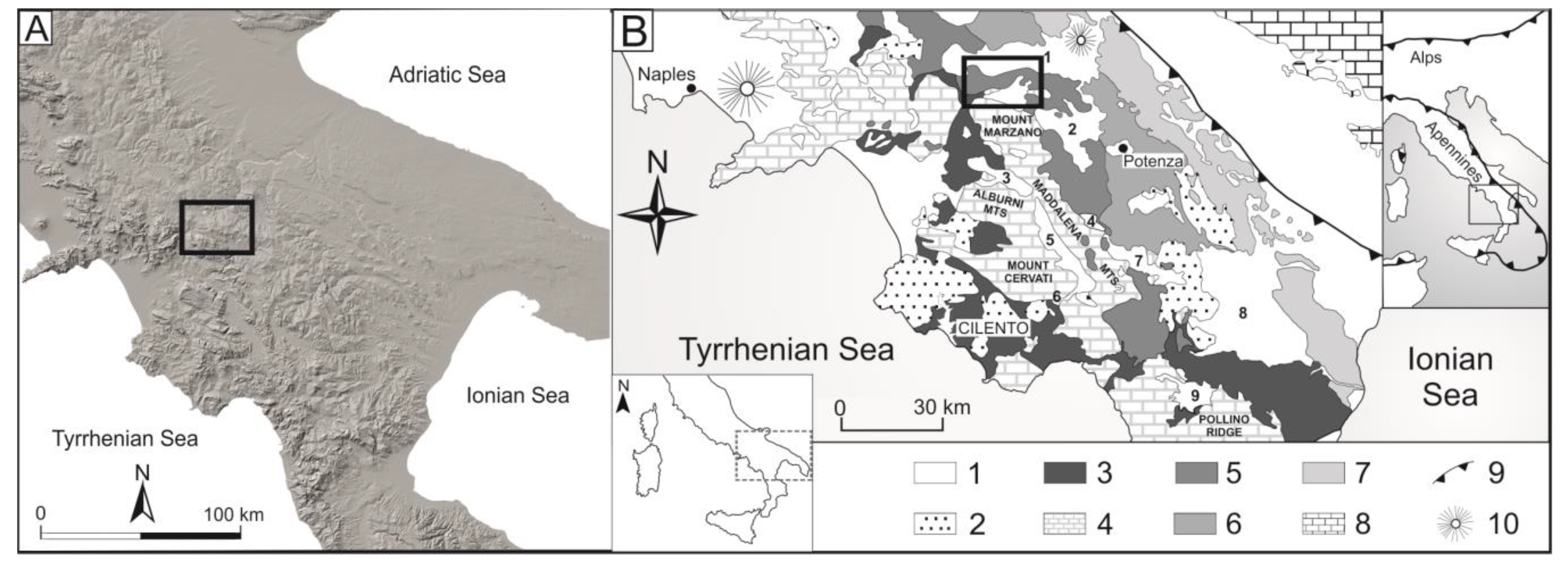
The test area is located in the southern sector of the Ofanto Basin, an intermontane tectonic depression of the axial-outer belt of the southern Apennines (Figure 1). The southern Apennines are a north-east verging fold-and-thrust belt, derived from the deformation of the western border of the Apulian plate [39,40]. Starting from the late Oligocene, the thrust belt involved the shallow- and deep-water sedimentary deposits of the African passive margin and Neogene-Pleistocene syntectonic and foredeep deposits [41]. The thrust front migrated progressively toward the north-east and was followed by a coeval back-arc extension [42], which is responsible for the opening of the Tyrrhenian sea and the extensional and strike-slip tectonics affecting the inner and axial domains of the chain [43,44]. Fold and thrust tectonics was responsible for the creation of different satellite basins, Pliocene in age, which are mainly located in the axial-outer belt of the chain. The latest stage of tectonic evolution of the chain is characterized by regional uplift and extensional faulting which occurred in Quaternary times and promoted the development of longitudinal and transversal intramontane depression in the axial-inner sectors of the belt [44,45,46].
The Ofanto basin is one of the larger intramontane depressions of the chain. It is an E–W trending structural low developed on poly-deformed Cretaceous to Miocene limestones, clays and sandstones of the Irpinian and Lagonegro units [47,48]. The basin is filled by a thick Pliocene to Pleistocene clastic succession (i.e., about 1000 m), made by marine to continental clay, sandstone and conglomerate that unconformably overlying the deformed pre-Pliocene bedrock [47,49]. The infill is intensely deformed by synsedimentary Pliocene-Quaternary folding and faulting and covers an elongate area of about 350 km2 along the present-day course of the Ofanto river [47].
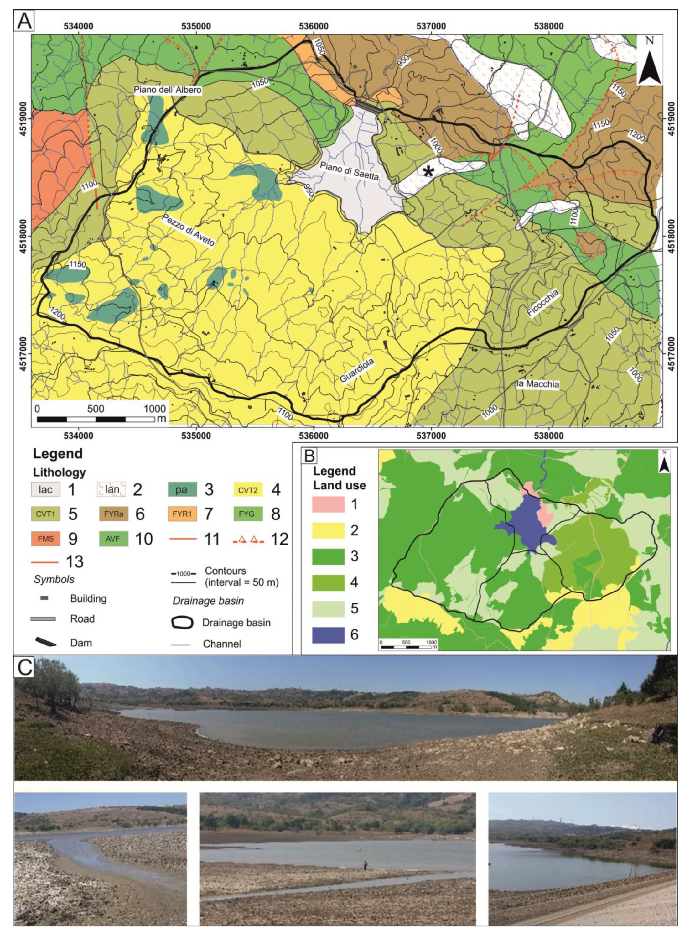
The study area is located in the headwaters of a small catchment drained by the Ficocchia stream, a tributary of the middle reach of the Ofanto River. The catchment is located in an upland area of the right-side of the Ofanto valley and is carved in a Cretaceous to Miocene bedrock succession composed by Lagonegro units, Sicilide calcareous-clay deposits and flysch deposits of Miocene syntectonic basins [47]. The upper Miocene deposits of the Castelvetere Formation. are the widespread rocks of the study area: they are mainly constituted by coarse- to medium-grained light brown sandstone with rare intercalation of lens of conglomerate (CVT1, Figure 2a) passing upward to silt and marly clay (CVT2, Figure 2a) containing decametric blocks of calcareous olistoliths (pa, Figure 2a). This succession unconformably overlies the Lagonegro tectonic units, which crop out in the north-eastern sectors of the study area. Lagonegro units are also represented by lower–middle Cretaceous siliceous marls and shales and upper Cretaceous to Oligocene marls and shales with calcarenites and calcirudites of the Flysch Rosso Formation. Lower Cretaceous varicoloured clays and marly clay (AVF, Figure 2a) and, subordinately, marls and shales with calcarenites and calcirudites (FMS, Figure 2a) also outcrop in the northern sectors of the study area [47]. Landslide deposits and reservoir sediments represent the youngest deposits of the study area.
3. Materials and Methods
The prediction ability of the LEM-based sedimentary budget estimation has been evaluated using a source to sink approach. In fact, a comparison between the total amount of eroded sediment volumes and the amount of sediment storage within the reservoir has been carried out in a relatively short-time period (i.e., about 20 years). A geographical information system (GIS)-supported statistical analysis of the spatial distribution of the erosion/deposition processes has been carried out and allowed us to reconstruct the spatial distribution of the topographic changes and the catchment sectors where erosion processes are more developed.
3.1. Sediment Storage in the Artificial Reservoir
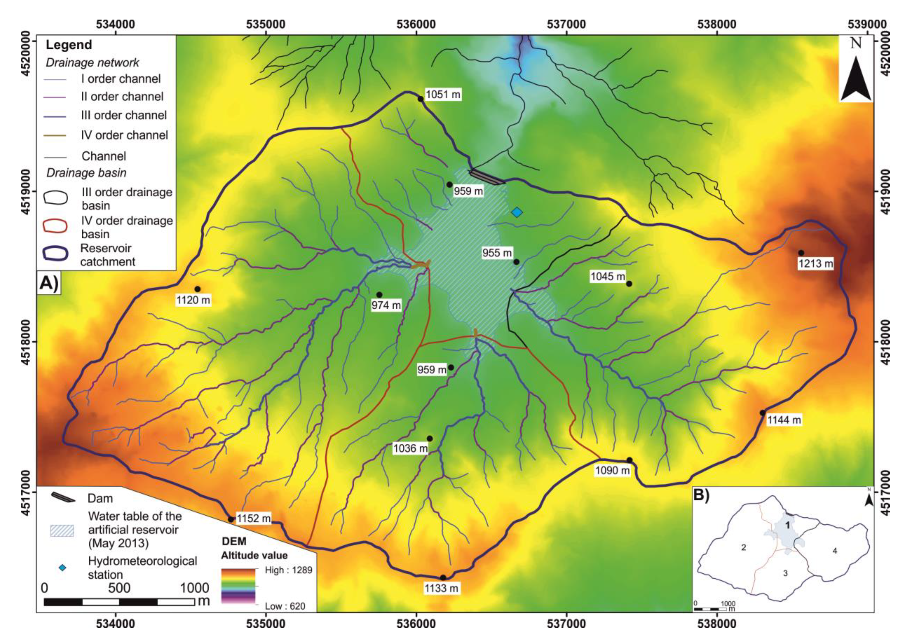
From 1988 to 1989, the EIPLI (Agency for the Development of the Irrigation and Agricultural Transformation, Ministry of Agricultural, Food and Forestry Policies) built up an earth dam (i.e., the Saetta dam) at the outlet of a small catchment located in the headwater sectors of the Ficocchia stream. The catchment of the artificial reservoir drains an area of about 9 km2 (Figure 3).
After about 18 years of dam activity, a bathymetric and seismo-acoustic survey was performed during a one-day field campaign in 1 September 2007, which allowed us to collect about 500 bathymetric points [50]. Horizontal control points have been extensively acquired by a Real Time Kinematic-Global Position System (RTK-GPS LEICA 1200 station whereas the elevation of the ground control point was referred to the estimated height of the reservoir water level. The amount of the sediment volumes stored in the dam was reconstructed on the basis of the comparison between the pre-existing topography and the sediment volumes estimated by the depth of the reservoir infill. Then, the reservoir sedimentation based on bathymetric and seismo-acoustic surveys was used in order to estimate the mean annual sediment deposition for the 1989–2007 period and a map of the sediment thickness has been created from the geostatistical interpolation of the collected bathymetric points [50]. Bathymetric survey was integrated by a geotechnical core drilling program [50], which allowed us to define the sediment density useful to define the specific sediment yield.
3.2. Caesar-Lisflood Landscape Evolution Model (LEM): Model Description and Parameterization
The Caesar–Lisflood LEM simulates landscape changes using a hydrological model to generate spatially distributed runoff, which is propagated on a regular grid of cells (i.e., the DEM of the study area) to estimate flow depths and velocities. This hydrodynamic model is used to modify elevations and estimates fluvial erosion and deposition within an active layer with peculiar grain-size features. Slope processes and soil creep are also included in the simulation [51]. In this work, the model has been used in the catchment mode with no internal influxes other than rainfall. The input data of the model includes DEM of the catchment, grain sizes, rainfall data, bedrock depth and value of Manning coefficient [35].
The model requires a rainfall precipitation input to generate runoff over the catchment, which controls the fluvial and hillslope processes and drives erosion and deposition for the modelled time step [35,51]. The modified topography becomes the starting point for the next time step. Flow depths and velocity are calculated from discharges between cells using Manning’s equation. These flow depths and velocities are then used to simulate the transport and deposition of sediment. Caesar estimates sediment transport over nine grain-size fractions, which can be transported either as bed load or as suspended load, depending on the user specification. Caesar provides the [52] or the [53] equations to estimate sediment transport.
Slope processes are also included, with mass movement when a critical slope angle threshold is exceeded, together with soil creep. These allow material from slopes to be fed into the fluvial system as well as the input from landslides and soil creep. After the fluvial erosion/deposition and slope process amounts are calculated, the elevations and grain size properties of the cells are updated. Outputs of the model are the elevation changes across the whole modelled topography as well as water discharges and sediment fluxes at the outlet over time.
An accurate definition of both the input data and model parameters is crucial to obtain a reliable predictive model. In order to provide a representative picture of the study area, the input parameters have been accurately derived from lithological, climate and land-use features of the Ficocchia stream catchment.
A synoptic scheme of the input data and model parameterization is reported in Table 1. Hourly rainfall data have been extracted from an hydro-meteorological station located at the outlet of the catchment (Figure 3). Available rainfall record covers a 22-year period ranging from 1994 to 2016 whereas the elapsed time between the dam construction and the bathymetric survey is about 17 years. Thus, the model has been set using a 17-year record (i.e., 1 January 1994–31 December 2011) of the hourly rainfall data.
Starting from a high-resolution DEM (i.e., grid cell of 5 m) of the study area deriving by a light detection and ranging (LIDAR) survey (http://rsdi.regione.basilicata.it/rbgeoserver2016/rsdi_wcs/dtm_5m/wcs), we have defined the bedrock depth through a detailed analysis of the outcropping lithological units. Firstly, a lithological map has been drawn from literature data and new field surveys (Figure 2). Field-based measurements of the soil depth have been done for the different lithological units and a mean estimation of soil thickness and bedrock depth has been reconstructed. This kind of information has been summarized in a soil thickness map (see Section 4.2), which has been used to define both the bedrock depth and grain-size features within the shallower active layer where erosion and deposition processes can occur. According to the estimated thickness of the soil depth for the different lithological units, an isopach map of the soil thickness has been derived for the different lithological units of the study area (see Section 4.1). Then, the bedrock map has been reconstructed using a GIS-supported subtraction between the reconstructed soil thickness and the DEM-deriving altitude data.
A recent work by [38] highlighted that there are only a limited number of parameters with a high degree of influence on the Caesar–Lisflood results. In particular, the application of sensitivity analysis suggests that model results are strongly influenced by the sediment transport formula and Manning coefficient. For this reason, these parameters have been carefully selected. Einstein’s sediment transport equation [52] was developed based on (predominantly) sand based laboratory channels and have been here chosen according to the grain-size features of the study area.
4. Results
4.1. Geomorphological Features
Landscape features of the study area are strictly related to the tectonic evolution and relief growth of this sector of the chain, which controlled in turn the distribution of the outcropping deposits. Landscape is featured by E–W trending morpho-structural ridges and thrust sheets, which are mainly carved in Cretaceous-to-Miocene pelagic deposits (Figure 2a). These landforms are transversally incised by a IV-order drainage basin (i.e., the Ficocchia stream), located in the right-side of the Ofanto river at an altitude ranging from 942 and 1242 m a.s.l. (Figure 3). The drainage basin of the artificial reservoir includes three small catchments of low hierarchical order, which are arranged in a sub-dendritic pattern. Drainage divide of the catchment of the southern sector shows an elongate shape and is developed on a gentle topography related to remnants of low-relief erosional land-surfaces [49]. Headwater channels of the southernmost sectors exhibit a moderate degree of hierarchization (Figure 3) and are featured by a higher gradient than the lower reaches. Fluvial processes related to the channel incision are the main geomorphological processes of the study area and represent the main controlling factors of the sediment flux. In fact, minor shallow landslides and small earthflows can be only observed in the eastern sectors of the catchment, where clay-rich lithological units crop out.
Land use of the study area deriving by a digital inventory of the Basilicata Region (http://rsdi.regione.basilicata.it) is shown in Figure 2b. Land use map roughly follows the classification scheme of the III level of the Corine Land Cover project [56] and highlights a clear prevalence of the semi-natural areas. Natural grasslands and sclerophyllous vegetations (frame 4 and 7 in Figure 2b) cover about the 80% of the total area; minor extent of agricultural areas and urban areas as buildings and roads cover the rest of the study area.
4.2. Regional Climate Setting and Local Rainfall Distribution
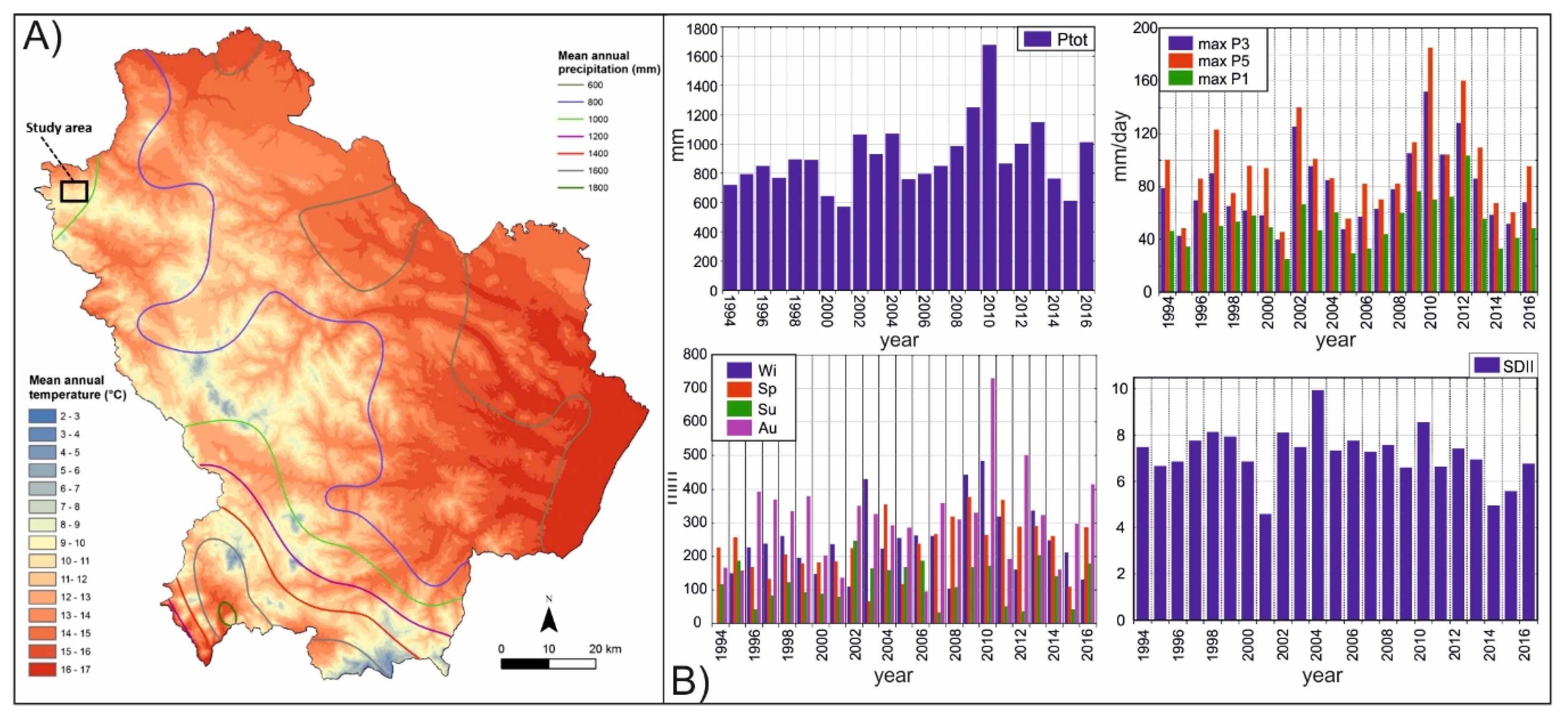
Statistical analysis of historical temperature and rainfall data has been performed using the daily rainfall data from a meteorological station located about 20 km to the west of the study area (i.e., Pescopagano weather station, rainfall record: 1951–2010). Climate record highlights a typical Mediterranean-type climate setting with dry summers and cold winters and peaks of extreme weather events in the autumn. The yearly average temperature ranges from 11.6 °C to 14.5 °C, with an average maximum between 18.6 °C and 24.5 °C during summer and an average minimum ranging between 3.2 °C and 8.0 °C during winter [57]. Considering the long-term variation of the temperature, Tmin shows upward trends in winter, spring and summer, whereas it shows downward trends in autumn, especially in the last normal 1981–2010, while Tmax also shows upward trends in spring and summer, whereas it tends to decrease during winter and autumn. A general upward tendency on warm days, warm nights, tropical nights, summer days and very warm days after 1971 is shown in [57]. The majority of cold extremes, i.e., very cold nights, cold days, cold nights and frost days showed negative trends, thus confirming the overall warming trend in the Basilicata region.
The average annual rainfall of the study area over the period 1951–2010 is higher than 1000 mm year−1 (Figure 4a). According to [58], the annual and seasonal total precipitation indicated a general downward trend over the 1951–2000 period, mainly due to the autumn–winter decrease of precipitation. In the last decade, rainfall record showed an increase in total rainfall and precipitation intensity and a small decrease in dry spell lengths [58]. Such a recent trend is due to multi-day extreme precipitations rather than to single-day precipitation. The increase in intensity/frequency of multi-days extreme events has led to the growth of severe soil loss and landslide events [59,60], not only in autumn and winter but even in the early spring [61].
Analysis of the shorter-term rainfall record (1994–2016) of the hydro-meteorological station of the artificial reservoir has been carried out through the estimation of several annual and seasonal precipitation indices [62]. As previously described in the Section 3.2, rainfall observations do not cover the overall time interval between the dam construction and the bathymetric survey. In fact, the hourly rainfall record starts about four years after the dam construction. In order to perform a LEM-based erosion estimation covering the same time-interval of the reservoir sediment storage, we decide to perform a 17-year simulation scenario starting from the available rainfall record (i.e., 1 January 1994–31 December 2011). Seasonal data show that the rains are mainly concentrated in the autumn and winter periods, with an average annual precipitation of 908 mm (Figure 4b). The maximum annual precipitation of 1674 mm occurred in 2010, which also represent the period with the greatest number of rainy days. A minimum of the cumulative annual rainfall of 569 mm has been recorded in 2001.
The cumulative precipitation over 5 days (P5) is for the most part represented by the amount of rain that falls in the first 24 h (P1) and in some cases in the first three days (P3). This highlights the role and the decisive contribution of extreme events, concentrated mostly in a few hours on the first day of rain, in the erosion processes active in this basin.
4.3. Reservoir Sediment Storage
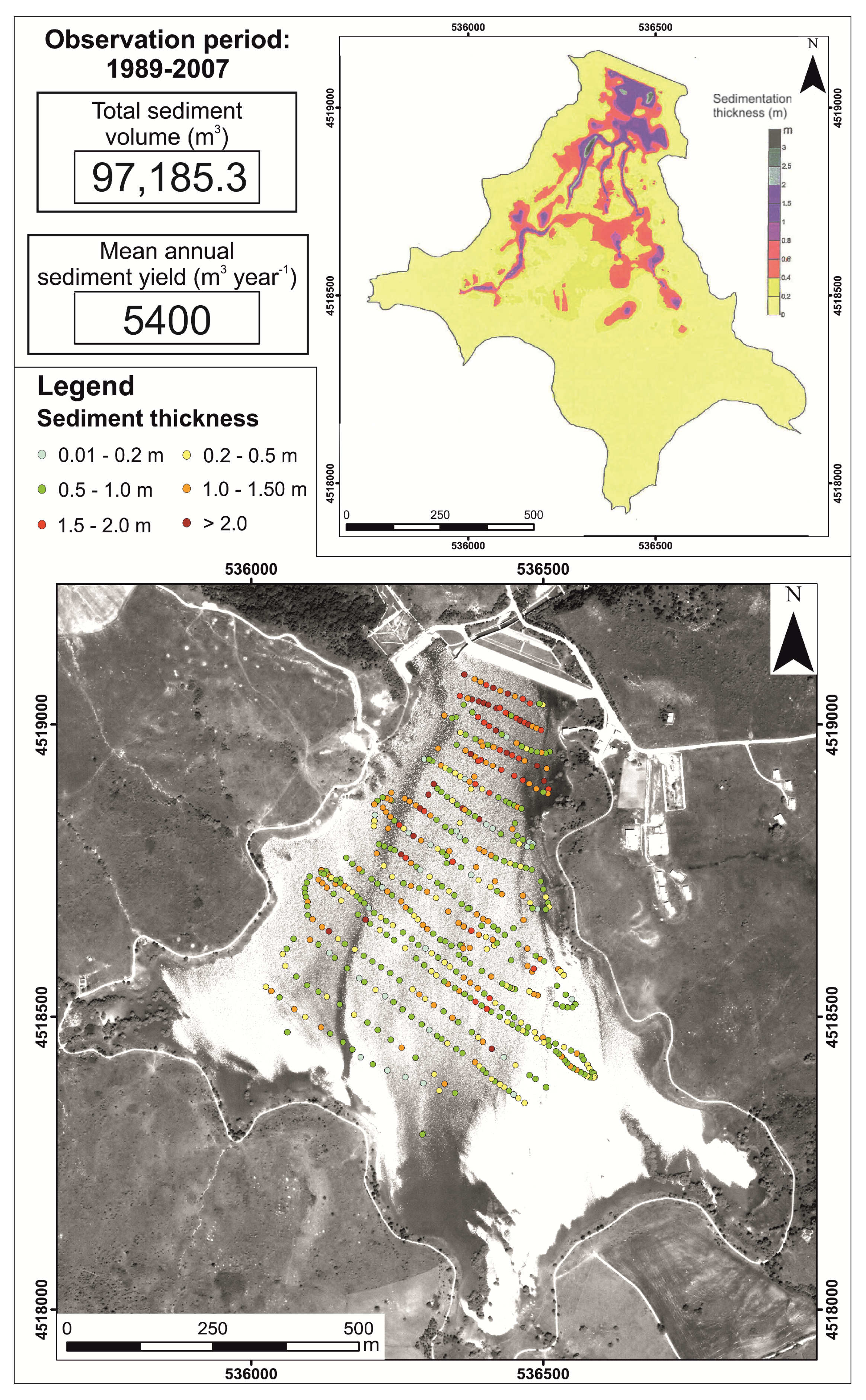
Historical data of sedimentation in the Saetta reservoir (i.e., 18 years) allowed an estimation of the total sedimentation in the reservoir in about 97,185.3 m3 (Figure 5).
The mean annual sediment yield is equal to 5400 m3/year. Grain-size analysis of the core samples acquired on the reservoir bottom indicate that the reservoir sediment infill is mainly constituted by silt and mud deposits. The bulk density of these sediments is 1.1 g/cm−3. Using this bulk density value, a mean annual specific sediment yield of 491.8 Mg km−2 year−1 can be reconstructed.
4.4. Caesar–Lisflood LEM
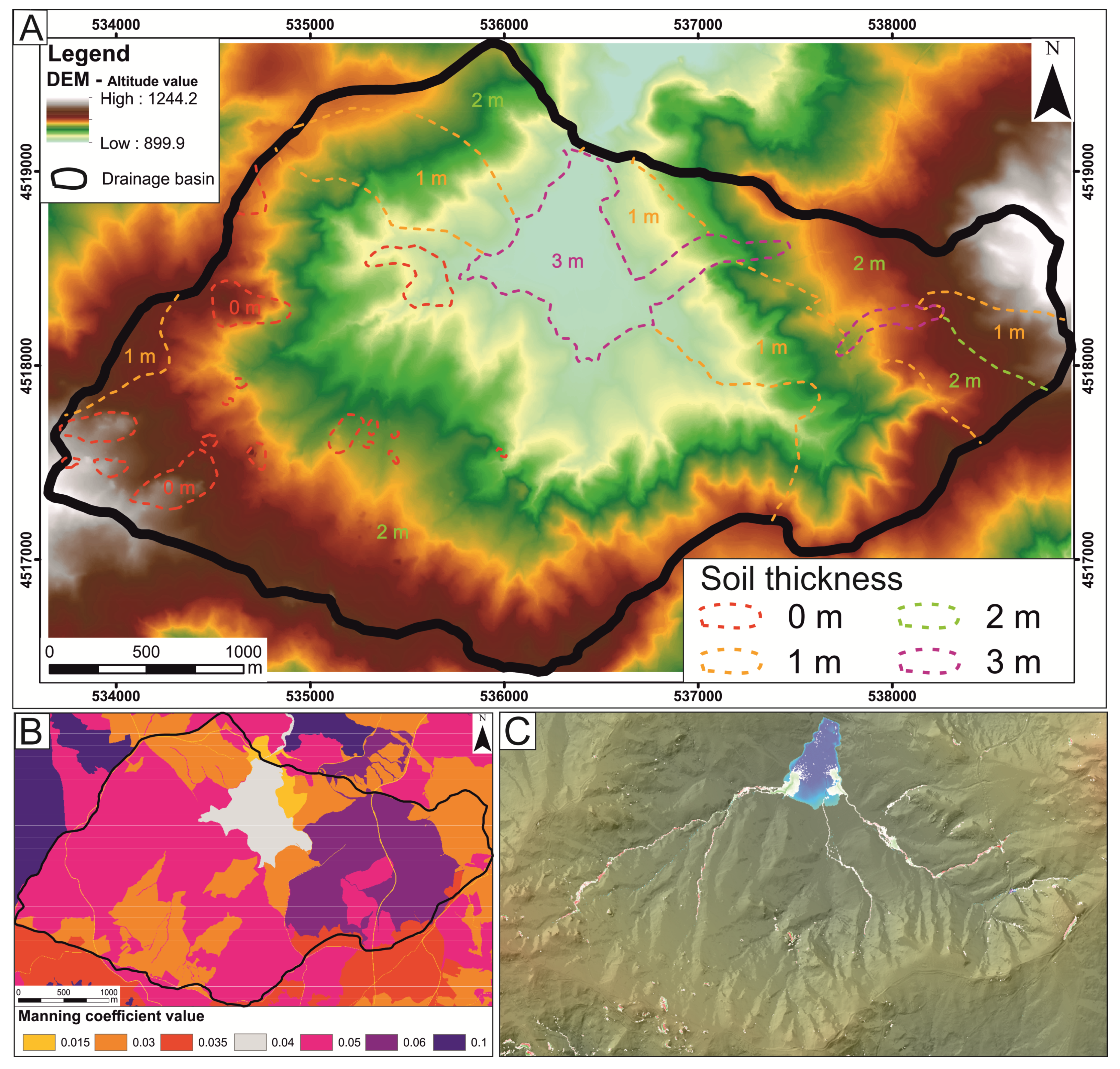
Caesar-Lisflood simulation outputs are analysed in a GIS environment in order to investigate the spatial distribution of erosion and deposition and its relationships with lithology, land use and geomorphological features. Figure 6 provides an overview of the main input and output data of the model. Figure 6a shows the DEM of the study area and the isopachs of the soil thickness. The contour map exhibits the maximum soil thickness of 3 m where Holocene deposits crop out whereas the bedrock has the same altitude of the DEM in correspondence of the carbonate rock outcrop (Figure 6a). A soil thickness ranging from 1 to 2 m has been reconstructed in the sectors featured by the other lithological units.
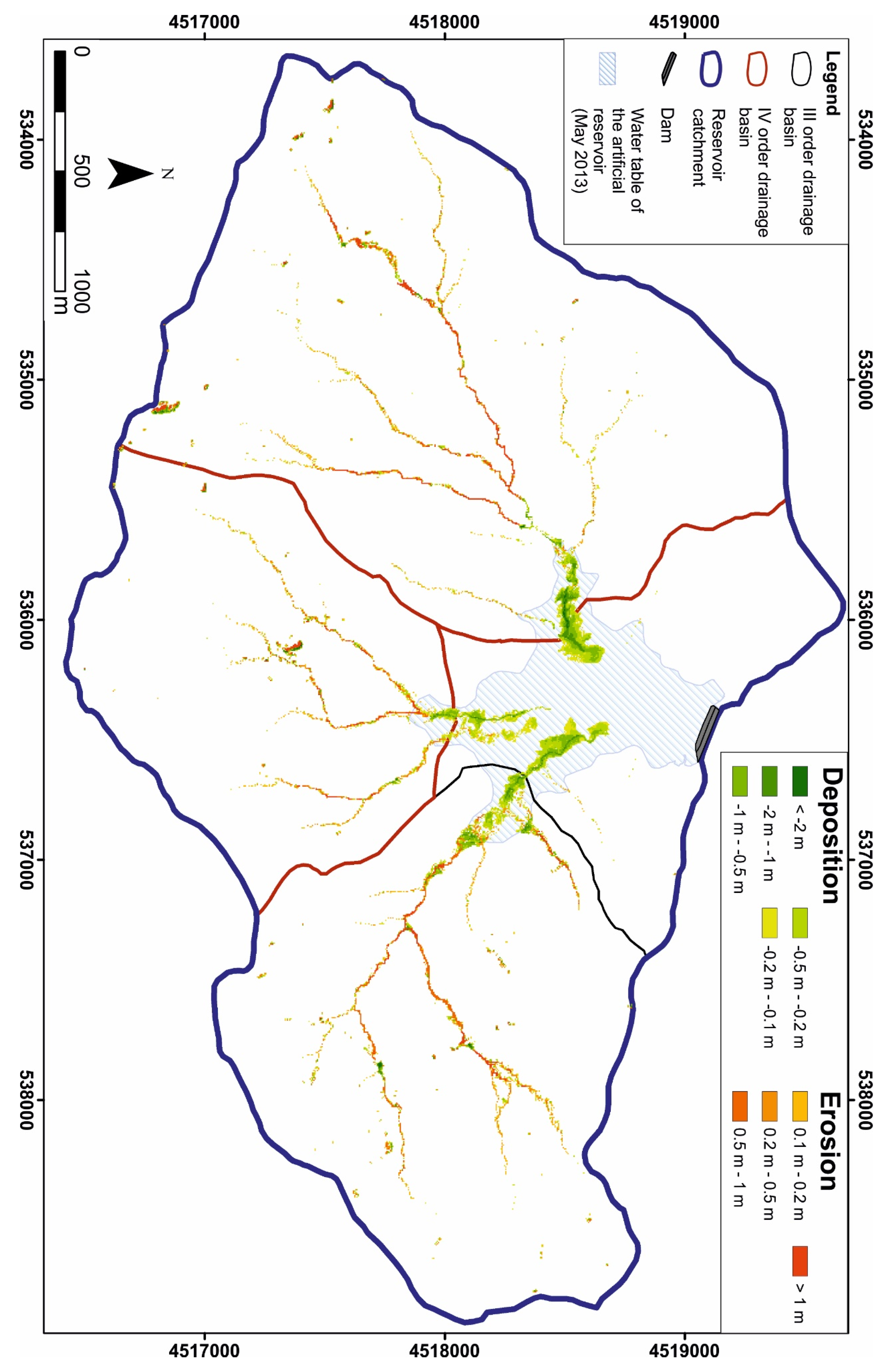
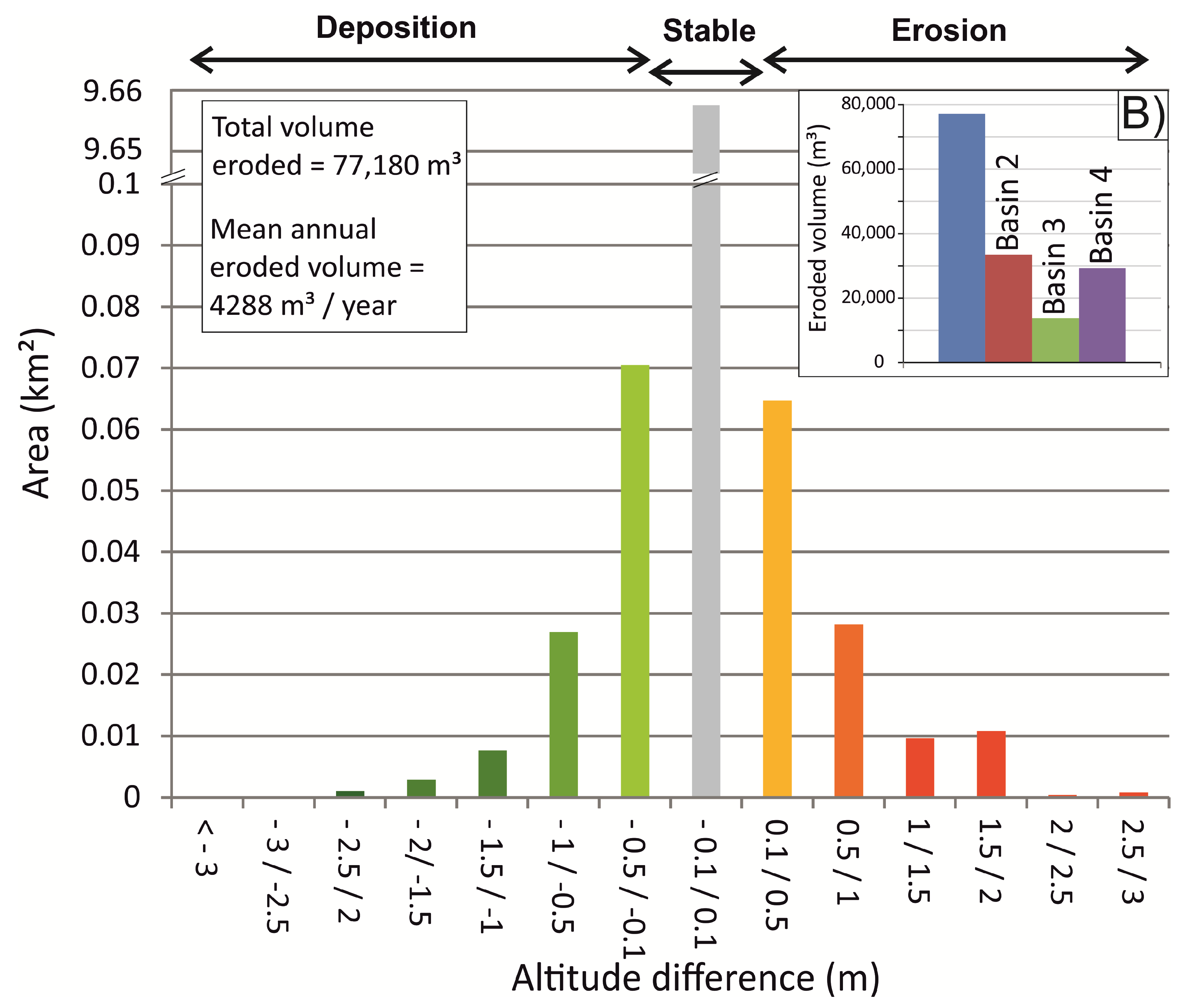
Figure 7 shows the results of the elevation changes caused by erosion and deposition after an 18-year simulation. The total amount of erosion predicted by Caesar–Lisflood LEM is equal to 77,180 m3, which correspond to a mean annual erosion volumes of 4288 m3/year.
Approximately 44.0% of the total amount of sediment eroded comes from the IV-order drainage basin (i.e drainage basin 2, Figure 8) whereas the smaller easternmost catchment contributes to the total sediment yield with a similar value (38%, drainage basin 4, Figure 8). Caesar–Lisflood simulation predicts topographic changes for an area of about 0.23 km2, which represent 2.3% of the total catchment area. Maximum depth of erosion is 3.8 m whereas erosion areas with a value ranging from 0.1 to 0.5 m are the prevalent class of the altitude difference map (i.e., about the 56% of the area affected by erosion, Figure 8).
Visual inspection of the LEM difference map indicates that erosion processes are mainly developed along the channels of the drainage network, which promoted the incision and the main topographic changes of the study area. Deposition cells are almost totally localized in the artificial reservoir, thus suggesting a value of sediment delivery ratio higher than 0.9 and a high degree of sediment connectivity. Local decreases of the channel gradient controlled the occurrence of minor deposition zones in the middle reach of the fluvial net. Results also predict a minor role of hillslope processes on the sediment yield of the study area.
5. Discussion and Concluding Remarks
LEM-based quantitative evaluation of the sediment budget of the Ficocchia drainage basin has been compared to a decadal-scale estimation of the deposition volumes in the Saetta reservoir. This kind of approach allowed us to verify the ability of the Caesar–Lisflood LEM to predict topographic changes, geomorphological processes and sediment flux in an upland catchment of the southern Apennine chain at a short-term temporal scale (i.e., 18 years).
A Caesar–Lisflood LEM requires a limited amount of input data (i.e., hourly rainfall record, DEM and soil particle size) for the simulation than traditional soil erosion models and many works have demonstrated its high potential to solve issue of sediment budget estimation, past and future landscape changes and analysis of geomorphological processes at different spatial and temporal scales [35,36,37,51]. Nevertheless, model applications are rather rare and limited to areas where a large amount of multiproxy data are available. The excessive number of parameters that are difficult to assess and assume as spatially and temporally homogeneous maybe represents the first reason for the rare application of such an approach. A recent work [38] investigated in detail the response of the Caesar–Lisflood LEM to the variation of the model parameters, testifying that only some parameters exert a relevant influence on the model results. In particular, most of them like Manning coefficient, sediment transport formula and grain size distributions can be accurately defined by detailed field measurements. In this work, we test for the first time the prediction ability of the Caesar–Lisflood LEM in a mountain catchment of the southern Italian Apennines. The model provided a reasonable estimation of erosion processes of 4288 m3 year−1, which is about 20% lower than the estimated annual sedimentation volumes from the bathymetric survey. The general good accordance between source-sink data testifies the reliability of the model results and highlights a high potential of a similar approach to solve issue of short-term landscape modification and sediment budget.
Then, the validation of the short-term prediction ability and the introduction of parameterisation (Table 1) for a complex Mediterranean-type landscape open a promising research field in applied geomorphology.
Results of the model appear to be in accordance also with the geomorphological evidences and spatial distribution of landforms and deposits revealed by multitemporal analysis of orthophotos and maps. In fact, geomorphological evidence such as V-shape of the channels and absence of slope and alluvial deposits along the channels well fit with the model results and confirm that channel incision are the main geomorphological processes controlling the sedimentation of the study area. Annual sediment yield from Caesar–Lisflood simulation is not linear and its variation (i.e., about the 15% of the long-term mean value) shows a positive correlation to the occurrence of extreme climate events. In particular, the model predicts erosion volumes of 5032 m3 and 4952 m3 for the 2010 and 2012, respectively. Thus, these peaks of annual sediment yield coincide with two years characterized by the occurrence of rainfall concentrated in a few days with very high intensity during the autumn season, as demonstrated by the analysis of the rainfall data (Figure 4).
In general, the comparison between erosion volumes from LEM simulation and field-based sedimentation data demonstrated a good prediction ability of the Caesar–Lisflood simulation although the model results seem to underestimate the field-based estimation of reservoir sedimentation. Estimation of sedimentation volume from bathymetric surveys could be affected by analytical errors which are hard to quantify, such as errors in ground control points and interpolation procedures of raw data. Nevertheless, we can reasonably argue that they introduce a negligible error in the mean annual estimation of sediment volume based on an 18-year history of the reservoir. Assuming a good degree of quality of the reservoir sedimentation data and a low impact of possible other source errors, results of our simulation suggest that the LEM-based estimation of sediment yield slightly underestimates the amount of sediment accumulation in the dam. This misfit could be attributed to the following concomitant factors: (i) a tendency of the Caesar–Lisflood LEM to underestimate slope processes. Creep and landslides are modelled as an instantaneous material movement related to overcoming a threshold and this relatively simple formulation could not be able to fully capture the hillslope processes of the study area. This issue has been already observed (see for example [35,63]) and could partly explain the slight difference between LEM-based sediment yield and sedimentation data. The crucial role of landslide phenomena (see [60] for some more details about the features and spatial distribution of landslide processes in the southern Apennine chain) in the increase of the sediment storage within a reservoir has been already demonstrated [1] and the earth-flow affecting the eastern sector of the artificial reservoir (see Figure 2) could represent a key element to reconcile modeling and field data; (ii) human-induced water-level oscillations of the reservoir have not been considered in the simulation; a lowering of the local base-level can promote fluvial incision and increase of sediment yield. Future works should deal with this possible source of model errors in order to improve the ability of the Caesar–Lisflood LEM to simulate complex landscapes subjected a human-induced variation of the base-level.
The encouraging results presented here testify that a Caesar–Lisflood LEM can represent an effective approach to estimate the sediment yield in Mediterranean-type landscape and its application in unmonitored landscapes can help to unravel the short-term morpho-dynamics of mountain catchments and the role of fluvial and hillslope processes in geomorphological evolution.
Author Contributions
Conceptualization, D.G.; methodology, D.G.; software, D.G.; validation, D.G.; formal analysis, D.G.; investigation, D.G., M.L.; resources, D.G., M.L.; data curation, D.G.; writing—original draft preparation, D.G.; writing—review and editing, D.G., M.L.; supervision, D.G., M.L.; project administration, D.G., M.L.; funding acquisition, M.L.
Funding
This research received no external funding.
Acknowledgments
We would like to thank the two anonymous referees for their useful comments and suggestions, which helped us to improve the manuscript. Moreover, we are grateful to Ing. Giovanni Di Trapani, manager of the Agency for the Development of the Irrigation and Agricultural Transformation E.I.P.L.I., Ministry of Agricultural, Food and Forestry Policies) for his technical and logistical support.
Conflicts of Interest
The authors declare no conflict of interest.
References
- Lazzari, M.; Gioia, D.; Piccarreta, M.; Danese, M.; Lanorte, A. Sediment yield and erosion rate estimation in the mountain catchments of the Camastra artificial reservoir (Southern Italy): A comparison between different empirical methods. CATENA 2015, 127, 323–339. [Google Scholar] [CrossRef]
- Borrelli, P.; Märker, M.; Panagos, P.; Schütt, B. Modeling soil erosion and river sediment yield for an intermountain drainage basin of the Central Apennines, Italy. CATENA 2014, 114, 45–58. [Google Scholar] [CrossRef]
- D’Oleire-Oltmanns, S.; Marzolff, I.; Peter, K.D.; Ries, J.B. Unmanned aerial vehicle (UAV) for monitoring soil erosion in Morocco. Remote Sens. 2012, 4, 3390–3416. [Google Scholar] [CrossRef]
- de Vente, J.; Poesen, J.; Verstraeten, G.; Van Rompaey, A.; Govers, G. Spatially distributed modelling of soil erosion and sediment yield at regional scales in Spain. Glob. Planet. Chang. 2008, 60, 393–415. [Google Scholar] [CrossRef]
- Capolongo, D.; Pennetta, L.; Piccarreta, M.; Fallacara, G.; Boenzi, F. Spatial and temporal variations in soil erosion and deposition due to land-levelling in a semi-arid area of Basilicata (Southern Italy). Earth Surf. Process. Landf. 2008, 33, 364–379. [Google Scholar] [CrossRef]
- Amore, E.; Modica, C.; Nearing, M.A.; Santoro, V.C. Scale effect in USLE and WEPP application for soil erosion computation from three Sicilian basins. J. Hydrol. 2004, 293, 100–114. [Google Scholar] [CrossRef]
- Merritt, W.S.; Letcher, R.A.; Jakeman, A.J. A review of erosion and sediment transport models. Environ. Model. Softw. 2003, 18, 761–799. [Google Scholar] [CrossRef]
- Tanyaş, H.; Kolat, Ç.; Süzen, M.L. A new approach to estimate cover-management factor of RUSLE and validation of RUSLE model in the watershed of Kartalkaya Dam. J. Hydrol. 2015, 528, 584–598. [Google Scholar] [CrossRef]
- Fernández, C.; Vega, J.A. Evaluation of the rusle and disturbed wepp erosion models for predicting soil loss in the first year after wildfire in NW Spain. Environ. Res. 2018, 165, 279–285. [Google Scholar] [CrossRef] [PubMed]
- Aiello, A.; Adamo, M.; Canora, F. Remote sensing and GIS to assess soil erosion with RUSLE3D and USPED at river basin scale in southern Italy. CATENA 2015, 131, 174–185. [Google Scholar] [CrossRef]
- Onori, F.; de Bonis, P.; Grauso, S. Soil erosion prediction at the basin scale using the revised universal soil loss equation (RUSLE) in a catchment of Sicily (southern Italy). Environ. Geol. 2006, 50, 1129–1140. [Google Scholar]
- Brown, A.G.; Carey, C.; Erkens, G.; Fuchs, M.; Hoffmann, T.; Macaire, J.-J.; Moldenhauer, K.-M.; Walling, D.E. From sedimentary records to sediment budgets: Multiple approaches to catchment sediment flux. Geomorphology 2009, 108, 35–47. [Google Scholar] [CrossRef]
- Jha, A.; Schkade, U.; Kirchner, G. Estimating short-term soil erosion rates after single and multiple rainfall events by modelling the vertical distribution of cosmogenic 7Be in soils. Geoderma 2015, 243–244, 149–156. [Google Scholar] [CrossRef]
- Polyakov, V.O.; Nearing, M.A.; Stone, J.J.; Holifield Collins, C.D.; Nichols, M.H. Quantifying decadal-scale erosion rates and their short-term variability on ecological sites in a semi-arid environment. CATENA 2016, 137, 501–507. [Google Scholar] [CrossRef]
- Mabit, L.; Benmansour, M.; Walling, D.E. Comparative advantages and limitations of the fallout radionuclides 137Cs, 210Pbex and 7Be for assessing soil erosion and sedimentation. J. Environ. Radioact. 2008, 99, 1799–1807. [Google Scholar] [CrossRef]
- Hancock, G.R.; Lowry, J.B.C.; Coulthard, T.J.; Evans, K.G.; Moliere, D.R. A catchment scale evaluation of the SIBERIA and CAESAR landscape evolution models. Earth Surf. Process. Landf. 2010, 35, 863–875. [Google Scholar] [CrossRef]
- Porto, P.; Walling, D.E. Using 137Cs and Pbex measurements to document erosion rates for different time windows in a small catchment in southern Italy. Hydrol. Process. 2013, 27, 297–302. [Google Scholar]
- Porto, P.; Walling, D.E. Use of caesium-137 measurements and long-term records of sediment load to calibrate the sediment delivery component of the SEDD model and explore scale effect: Examples from southern Italy. J. Hydrol. Eng. 2015, 20. [Google Scholar] [CrossRef]
- Beven, K. Changing ideas in hydrology—The case of physically-based models. J. Hydrol. 1989, 105, 157–172. [Google Scholar] [CrossRef]
- del Monte, M.; Vergari, F.; Brandolini, P.; Capolongo, D.; Cevasco, A.; Ciccacci, S.; Conoscenti, C.; Fredi, P.; Melelli, L.; Rotigliano, E.; et al. Multi-method evaluation of denudation rates in small mediterranean catchments. In Engineering Geology for Society and Territory—Volume 1: Climate Change and Engineering Geology; Springer: Cham, Switzerland, 2015; pp. 563–567. [Google Scholar]
- Ciccacci, S.; Fredi, F.; Palmieri, E.L.; Pugliese, F. Contributo dell’analisi geomorfica quantitativa alla valutazione dell’entita dell’erosione nei bacini fluviali. Boll. Della Soc. Geol. Ital. 1980, 99, 455–516. [Google Scholar]
- Gioia, D.; Martino, C.; Schiattarella, M. Long- to short-term denudation rates in the southern Apennines: Geomorphological markers and chronological constraints. Geol. Carpathica 2011, 62, 27–41. [Google Scholar] [CrossRef]
- Grauso, S.; Pasanisi, F.; Tebano, C.; Grillini, M.; Peloso, A. Investigating the Sediment Yield Predictability in Some Italian Rivers by Means of Hydro-Geomorphometric Variables. Geosciences 2018, 8, 249. [Google Scholar] [CrossRef]
- De Vente, J.; Poesen, J.; Bazzoffi, P.; Van Rompaey, A.; Verstraeten, G. Predicting catchment sediment yield in Mediterranean environments: The importance of sediment sources and connectivity in Italian drainage basins. Earth Surf. Process. Landf. 2006, 31, 1017–1034. [Google Scholar] [CrossRef]
- Mulder, T.; Syvitski, J.P.M. Climatic and morphologic relationships of rivers: Implications of sea-level fluctuations on river loads. J. Geol. 1996, 104, 509–523. [Google Scholar] [CrossRef]
- Poesen, J.; Nachtergaele, J.; Verstraeten, G.; Valentin, C. Gully erosion and environmental change: Importance and research needs. CATENA 2003, 50, 91–133. [Google Scholar] [CrossRef]
- Pieri, L.; Bittelli, M.; Wu, J.Q.; Dun, S.; Flanagan, D.C.; Pisa, P.R.; Ventura, F.; Salvatorelli, F. Using the Water Erosion Prediction Project (WEPP) model to simulate field-observed runoff and erosion in the Apennines mountain range, Italy. J. Hydrol. 2007, 336, 84–97. [Google Scholar] [CrossRef]
- Terranova, O.; Antronico, L.; Coscarelli, R.; Iaquinta, P. Soil erosion risk scenarios in the Mediterranean environment using RUSLE and GIS: An application model for Calabria (southern Italy). Geomorphology 2009, 112, 228–245. [Google Scholar] [CrossRef]
- Zingaro, M.; Refice, A.; Giachetta, E.; D‘Addabbo, A.; Lovergine, F.; De Pasquale, V.; Pepe, G.; Brandolini, P.; Cevasco, A.; Capolongo, D. Sediment mobility and connectivity in a catchment: A new mapping approach. Sci. Total Environ. 2019, 672, 763–775. [Google Scholar] [CrossRef]
- Cappadonia, C.; Coco, L.; Buccolini, M.; Rotigliano, E. From Slope Morphometry to Morphogenetic Processes: An Integrated Approach of Field Survey, Geographic Information System Morphometric Analysis and Statistics in Italian Badlands. Land Degrad. Dev. 2016, 27, 851–862. [Google Scholar] [CrossRef]
- Brandolini, P.; Pepe, G.; Capolongo, D.; Cappadonia, C.; Cevasco, A.; Conoscenti, C.; Marsico, A.; Vergari, F.; Del Monte, M. Hillslope degradation in representative Italian areas: Just soil erosion risk or opportunity for development? Land Degrad. Dev. 2018, 29, 3050–3068. [Google Scholar] [CrossRef]
- Aucelli, P.P.C.; Conforti, M.; Della Seta, M.; Del Monte, M.; D’Uva, L.; Rosskopf, C.M.; Vergari, F. Multi-temporal Digital Photogrammetric Analysis for Quantitative Assessment of Soil Erosion Rates in the Landola Catchment of the Upper Orcia Valley (Tuscany, Italy). Land Degrad. Dev. 2016, 27, 1075–1092. [Google Scholar] [CrossRef]
- Piacentini, T.; Galli, A.; Marsala, V.; Miccadei, E. Analysis of soil erosion induced by heavy rainfall: A case study from the NE Abruzzo Hills Area in Central Italy. Water (Switzerland) 2018, 10, 1314. [Google Scholar] [CrossRef]
- Coulthard, T.J.; Neal, J.C.; Bates, P.D.; Ramirez, J.; de Almeida, G.A.M.; Hancock, G.R. Integrating the LISFLOOD-FP 2D hydrodynamic model with the CAESAR model: Implications for modelling landscape evolution. Earth Surf. Process. Landf. 2013, 38, 1897–1906. [Google Scholar] [CrossRef]
- Coulthard, T.J.; Hancock, G.R.; Lowry, J.B.C. Modelling soil erosion with a downscaled landscape evolution model. Earth Surf. Process. Landf. 2012, 37, 1046–1055. [Google Scholar] [CrossRef]
- Coulthard, T.J.; van de Wiel, M.J. Modelling long term basin scale sediment connectivity, driven by spatial land use changes. Geomorphology 2017, 277, 265–281. [Google Scholar] [CrossRef]
- Hancock, G.R.; Coulthard, T.J.; Martinez, C.; Kalma, J.D. An evaluation of landscape evolution models to simulate decadal and centennial scale soil erosion in grassland catchments. J. Hydrol. 2011, 398, 171–183. [Google Scholar] [CrossRef]
- Skinner, C.J.; Coulthard, T.J.; Schwanghart, W.; Van De Wiel, M.J.; Hancock, G. Global sensitivity analysis of parameter uncertainty in landscape evolution models. Geosci. Model Dev. 2018, 11, 4873–4888. [Google Scholar] [CrossRef]
- Pescatore, T.; Renda, P.; Schiattarella, M.; Tramutoli, M. Stratigraphic and structural relationships between Meso-Cenozoic Lagonegro basin and coeval carbonate platforms in southern Apennines, Italy. Tectonophysics 1999, 315, 269–286. [Google Scholar] [CrossRef]
- Noguera, A.M.; Rea, G. Deep structure of the Campanian-Lucanian Arc (Southern Apennine, Italy). Tectonophysics 2000, 324, 239–265. [Google Scholar] [CrossRef]
- Patacca, E.; Scandone, P. Geology of the Southern Apennines. Boll. Della Soc. Geol. Ital. Suppl. 2007, 7, 75–119. [Google Scholar]
- Malinverno, A.; Ryan, W.B.F. Extension in the Tyrrhenian Sea and shortening in the Apennines as result of arc migration driven by sinking of the lithosphere. Tectonics 1986, 5, 227–245. [Google Scholar] [CrossRef]
- Cinque, A.; Patacca, E.; Scandone, P.; Tozzi, M. Quaternary kinematic evolution of the southern Apennines. Relationships between surface geological features and deep lithospheric structures. Ann. Geophys. 1993, 36, 249–260. [Google Scholar]
- Schiattarella, M.; Giano, S.I.; Gioia, D. Long-term geomorphological evolution of the axial zone of the Campania-Lucania Apennine, southern Italy: A review. Geol. Carpathica 2017, 68, 57–67. [Google Scholar] [CrossRef]
- Giano, S.I.; Gioia, D.; Schiattarella, M. Morphotectonic evolution of connected intermontane basins from the southern Apennines, Italy: The legacy of the pre-existing structurally controlled landscape. Rend. Lincei 2014, 25, 241–252. [Google Scholar] [CrossRef]
- Gioia, D.; Schiattarella, M.; Mattei, M.; Nico, G. Quantitative morphotectonics of the Pliocene to Quaternary Auletta basin, southern Italy. Geomorphology 2011, 134, 326–343. [Google Scholar] [CrossRef]
- Schiattarella, M.; Romeo, M.; Marino, M.; Giannandrea, P. Pliocene to Quaternary evolution of the Ofanto Basin in southern Italy: An approach based on the unconformity-bounded stratigraphic units. Ital. J. Geosci. 2014, 133, 27–44. [Google Scholar]
- Casciello, E.; Esestime, P.; Cesarano, M.; Pappone, G.; Snidero, M.; Verges, J. Lower plate geometry controlling the development of a thrust-top basin: The tectonosedimentary evolution of the Ofanto basin (Southern Apennines). J. Geol. Soc. 2013, 170, 147–158. [Google Scholar] [CrossRef]
- Labella, R.; Capolongo, D.; Giannandrea, P.; Giano, S.I.; Schiattarella, M. Morphometric analysis of fluvial network and age constraints of terraced surfaces of the Ofanto basin, Southern Italy. Rend. Lincei 2014, 25, 253–263. [Google Scholar] [CrossRef]
- Bazzoffi, P. Progetto REL: Attività tecnico-scientifiche “Assistenza tecnica e supporto agli enti concessionari nel settore dell’uso irriguo delle risorse idriche”, Rilievi batimetrici e sedimentologici dell’invaso Saetta; Centro per l’Agrobiologia e la Pedologia, CREA: Rome, Italy, 2008. [Google Scholar]
- Coulthard, T.J.; van de Wiel, M.J. Climate, tectonics or morphology: What signals can we see in drainage basin sediment yields? Earth Surf. Dyn. 2013, 1, 13–27. [Google Scholar] [CrossRef]
- Einstein, H.A. The Bed-Load Function for Sediment Transportation in Open Channel Flows. Soil Conserv. Serv. 1950, 1026, 1–31. [Google Scholar]
- Peter, R.W.; Joanna, C.C. Surface-based Transport Model for Mixed-Size Sediment. J. Hydraul. Eng. 2003, 129, 120–128. [Google Scholar]
- Ding, Y.; Jia, Y.; Sam, S.Y.W. Identification of Manning’s Roughness Coefficients in Shallow Water Flows. J. Hydraul. Eng. 2004, 130, 501–510. [Google Scholar] [CrossRef]
- Phillips, J.V.; Tadayon, S. Selection of Manning’s Roughness Coefficient for Natural and Constructed Vegetated and Non-Vegetated Channels, and Vegetation Maintenance Plan Guidelines for Vegetated Channels in Central Arizona; Report 2006-5108; U.S. Geological Survey: Reston, VA, USA, 2006.
- Büttner, G. CORINE Land Cover and Land Cover Change Products. In Land Use and Land Cover Mapping in Europe: Practices & Trends; Manakos, I., Braun, M., Eds.; Springer: Dordrecht, The Netherlands, 2014; pp. 55–74. [Google Scholar]
- Piccarreta, M.; Lazzari, M.; Pasini, A. Trends in daily temperature extremes over the Basilicata region (southern Italy) from 1951 to 2010 in a Mediterranean climatic context. Int. J. Climatol. 2015, 35, 1964–1975. [Google Scholar] [CrossRef]
- Piccarreta, M.; Pasini, A.; Capolongo, D.; Lazzari, M. Changes in daily precipitation extremes in the Mediterranean from 1951 to 2010: The Basilicata region, southern Italy. Int. J. Climatol. 2013, 33, 3229–3248. [Google Scholar] [CrossRef]
- Lazzari, M.; Gioia, D. Regional-scale landslide inventory, central-western sector of the Basilicata region (Southern Apennines, Italy). J. Maps 2016, 12, 852–859. [Google Scholar] [CrossRef]
- Lazzari, M.; Gioia, D.; Anzidei, B. Landslide inventory of the Basilicata region (Southern Italy). J. Maps 2018, 14, 348–356. [Google Scholar] [CrossRef]
- Clarke, M.L.; Rendell, H.M. Hindcasting extreme events: The occurrence and expression of damaging floods and landslides in Southern Italy. Land Degrad. Dev. 2006, 17, 365–380. [Google Scholar] [CrossRef]
- WMO. Calculation of Monthly and Annual 30-Year Standard Normals; WCDP No. 10, WMO-TD/No. 341; WMO: Geneva, Switzerland, 1989. [Google Scholar]
- Hoober, D.; Svoray, T.; Cohen, S. Using a landform evolution model to study ephemeral gullying in agricultural fields: The effects of rainfall patterns on ephemeral gully dynamics. Earth Surf. Process. Landf. 2017, 42, 1213–1226. [Google Scholar] [CrossRef]
Figure 1.
(A) Location of the study area in the frame of the southern Italian landscape. (B) Geological sketch map of the southern Apennines. The study area is represented in the box. Legend: (1) Pliocene to Quaternary clastic deposits and volcanic products; (2) Miocene syntectonic deposits; (3) Cretaceous to Oligocene ophiolite-bearing internal units; (4) Mesozoic–Cenozoic shallow-water carbonates of the Apennines platform; (5) lower–middle Triassic to Miocene shallow-water and deep-sea successions of the Lagonegro-typeMonte Arioso unit; (6)Mesozoic to Miocene deep-sea successions of the Lagonegro-type Groppa d’Anzi unit; (7) Cretaceous to Miocene deep-sea successions of the Lagonegro-type Campomaggiore unit; (8) Mesozoic–Cenozoic shallow-water carbonates of the Apulian platform; (9) thrust front of the chain; (10) volcanoes.

Figure 2.
Physical features of the study area. (A) Geological map of the study area (modified from [47]). Legend: (1) Fine-grained sediments of lacustrine environment (lac, Holocene) (2) Landslide deposits (lan, Holocene) (3) Decametric blocks of mudstone (pa, Upper Miocene); (4) Silt and marly clay (CVT2, Upper Miocene); (5) Coarse- to medium-grained light brown sandstone with rare intercalation of 1 to 6 thick lens of polygenic conglomerate (CVT1, Upper Miocene); (6) Calcareous breccia and grey shale (FYRa, Lower Cretaceous-Oligocene); (7) Chert, marly clay with intercalation of calcarenites and calcareous breccia (FYR1, Lower Cretaceous-Oligocene); (8) Light-grey and greenish shale with intercalation of thin beds of marls and marly limestone (FYG, Lower Cretaceous); (9) Alternance of calcarenite, calcilutite with nodular chert and varicoloured clay (FMS, Upper Cretaceous-Eocene); (10) Varicoloured clay (AVF, Lower Cretaceous); (11) High-angle fault (dashed if uncertain); (12) Thrust (dashed if uncertain); (13) Stratigraphic contact. The asterisk highlights a landslide representing a probable key-element in reservoir sediment flux. (B) Land use map. Legend: (1) Anthropic surfaces and roads; (2) Arable lands; (3) Sclerophyllous vegetation; (4) Broad-leaved and mixed forests; (5) Natural grasslands; (6) Water courses and water bodies. (C) Panoramic views showing the artificial reservoir and the surrounding sectors.

Figure 3.
(A) Drainage network of the study area and relative hierarchization according to the Strahler’s orders. Hydro-meterological station (coordinates: 40.8207° N; 15.4338° E) is also shown. (B) Numbering of the drainage basin.
Figure 3.
(A) Drainage network of the study area and relative hierarchization according to the Strahler’s orders. Hydro-meterological station (coordinates: 40.8207° N; 15.4338° E) is also shown. (B) Numbering of the drainage basin.

Figure 4.
Regional and local climate setting. (A) Climate map of the Basilicata region showing the mean annual temperature and rainfall for the 1951–2010 period (Source: Pescopagano weather station); (B) Precipitation indices deriving by the hourly rainfall record of the dam weather station. Legend: Ptot: annual rainfall; annual maximum rainfall for 1 (P1), 3(P3) and 5(P5) days. Wi: Winter; Sp: Spring; Su: Summer; Au: Autumn. SDII: simple daily intensity index representing the ratio between the total annual precipitation and the number of annual rainy days.

Figure 5.
Bathymetric survey carried out 18 years after the building of the dam. Sedimentation volume has been reconstructed by comparing a pre-dam topography (year: 1987) with the interpolated map of the sediment thickness deriving from the results of the bathymetric survey (September 2007).
Figure 5.
Bathymetric survey carried out 18 years after the building of the dam. Sedimentation volume has been reconstructed by comparing a pre-dam topography (year: 1987) with the interpolated map of the sediment thickness deriving from the results of the bathymetric survey (September 2007).

Figure 6.
Examples of the input and output data of the Caesar-Lisflood simulation scenario. (A) Digital elevation model (DEM) of the study area (spatial resolution: 5 m) and isopachs of the soil thickness extracted by geostatistical interpolation of the field-survey measurements. (B) Spatial distribution of the Manning coefficient values deriving by the land use map. (C) Intermediate output of the simulation (31 December 1995) showing: (i) the river water levels (white tones); (ii) erosion (red tones) and deposition (green tones) pattern; (iii) reservoir water level (blue tones).

Figure 7.
Elevation difference map deriving by the Caesar–Lisflood landscape evolution model (LEM).

Figure 8.
Histogram showing the distribution of the erosion/deposition classes deriving from the geographical information system (GIS)-supported analysis of the altitude difference map.
Figure 8.
Histogram showing the distribution of the erosion/deposition classes deriving from the geographical information system (GIS)-supported analysis of the altitude difference map.


Table 1.
Model parameters.
| Number | Caesar–Lisflood Parameter | Value |
|---|---|---|
| 1 | Grainsizes (m) | 0.0005, 0.001, 0.002, 0.004, 0.008, 0.016, 0.032, 0.064, 0.128 |
| 2 | Grainsize proportions (total 1) | 0.20, 0.18, 0.12, 0.06, 0.03, 0.03, 0.1, 0.25 |
| 3 | Rainfall timestep | hourly |
| 4 | Sediment transport law | Einstein |
| 5 | Max erode limit (m) | 0.01 |
| 6 | Active layer thickness (m) | 0.1 |
| 7 | Lateral edge smoothing passes | 40 |
| 8 | Manning coefficient | 0.015–0.1—Land-use map |
| 9 | Soil creep/diffusion value | 0.0025 |
| 10 | Slope failure threshold | 40 |
| 11 | Vegetation critical stress | 100 |
Table 2.
Manning coefficient.
| Number | Land-Use Cover | Manning Coefficient |
|---|---|---|
| 1 | Anthropic surfaces and roads | 0.015 |
| 2 | Arable lands | 0.035 |
| 3 | Sclerophyllous vegetation | 0.05 |
| 4 | Broad-leaved and mixed forests | 0.1 |
| 5 | Natural grasslands | 0.03 |
| 6 | Water courses and water bodies | 0.04 |
© 2019 by the authors. Licensee MDPI, Basel, Switzerland. This article is an open access article distributed under the terms and conditions of the Creative Commons Attribution (CC BY) license (http://creativecommons.org/licenses/by/4.0/).
Share and Cite
MDPI and ACS Style
Gioia, D.; Lazzari, M. Testing the Prediction Ability of LEM-Derived Sedimentary Budget in an Upland Catchment of the Southern Apennines, Italy: A Source to Sink Approach. Water 2019, 11, 911. https://doi.org/10.3390/w11050911
AMA Style
Gioia D, Lazzari M. Testing the Prediction Ability of LEM-Derived Sedimentary Budget in an Upland Catchment of the Southern Apennines, Italy: A Source to Sink Approach. Water. 2019; 11(5):911. https://doi.org/10.3390/w11050911
Chicago/Turabian StyleGioia, Dario, and Maurizio Lazzari. 2019. "Testing the Prediction Ability of LEM-Derived Sedimentary Budget in an Upland Catchment of the Southern Apennines, Italy: A Source to Sink Approach" Water 11, no. 5: 911. https://doi.org/10.3390/w11050911
Note that from the first issue of 2016, this journal uses article numbers instead of page numbers. See further details here.