The Use of Hydrodynamic Models in the Determination of the Chart Datum Shape in a Tropical Estuary
by
 , ,
, ,
Carlos Zapata
1,2,* ,
,
Araceli Puente
2,
Andrés García
2, 
Javier García-Alba
2 and 
Jorge Espinoza
1 1
Department of Hydrography, Instituto Oceanográfico de la Armada (INOCAR), Guayaquil 090208, Ecuador
2
Environmental Hydraulics Institute, Universidad de Cantabria, 39005 Santander, Spain
*
Author to whom correspondence should be addressed.
Water 2019, 11(5), 902; https://doi.org/10.3390/w11050902
Submission received: 7 March 2019
/
Revised: 17 April 2019
/
Accepted: 20 April 2019
/
Published: 29 April 2019
(This article belongs to the Section Hydraulics and Hydrodynamics)
Abstract
:Estuaries are transitional environments with ideal conditions for port construction and navigation. They represent a challenge to hydrographic services due to the dynamics of the seabed and the tidal wave deformation. The bottom slope, the convergence of the channels, and the nonlinear effects produced by the bottom friction produce variation in both the tidal range and the location of the chart datum (CD). In this study, sea level data series obtained from the nodes of the mesh of a hydrodynamic model (virtual tide gauges) were used to calculate the harmonic constituents, form factor, asymmetry, and estuary type. The final chart datum surface, obtained from the hydrodynamic model, was used to determine the separation values between zones and also the number of tidal zones in an estuarine system. It was found that in a complex hydrodynamics scenario, the use of the ellipsoidal referenced surveying (ERS) method is more convenient than traditional tidal zoning survey. In the ERS method, once the CD model is complete, it must be attached to the ellipsoid directly. Finally, the variation of the CD in different scenarios (due to anthropogenic action) was assessed.
1. Introduction
Estuaries are complex transitional environments [1], as they constitute the interface between ocean and river environments as well as marine and terrestrial systems. As a result, they provide a significant variety of physical, chemical, and geomorphological environmental conditions [2,3]. They are ideal locations for the construction of ports, harbors, and shipyards, since they provide appropriate conditions for navigation, maneuvering, and the sheltering of ships [4,5].
Estuaries represent a unique challenge for hydrographic services due to the dynamics of the seabed and the variation of the tidal wave, which is generated in the ocean, crosses the continental shelf, and reaches the estuaries [6]. The bottom friction, full and partial reflection, geometry, and seasonal river discharge of the estuaries determine the tidal range, the magnitude of the tidal currents, and the importance of the harmonic constituents of the tidal wave [7,8]. Characterization of the tide (amplitude and phase patterns of the main tidal constituents, form factor, and tidal asymmetry) provides important information for hydrographic activities. Tidal distortion influences navigability in estuarine channels and the geomorphological evolution of estuaries [9]. Characterization of the tide could be done by a hydrodynamic modelling or data-driven approach (DDA) [10]. The hydrodynamic models produce a numerical solution of one or more of the governing differential equations of continuity, momentum, and energy of fluid [11,12], while the DDA helps us to find coherent patterns of temporal behavior that could be used to characterize physical processes [10].
The determination of the chart datum (CD) is also derived from the characterization of the tide. The CD is the reference level to which the depths refer (level = 0), and it is used for the tide correction in a hydrographic survey. Due to the varying tidal characteristics, a large number of implementations of CD exist, such as mean lower low water springs (MLLWS), mean lower low water (MLLW), mean low water (MLW), low water (LW), lowest astronomical tide (LAT), and mean low water springs (MLWS) [13]. The spatial variation of the tidal range and the bottom slope in rivers [14] causes a change in the location of the CD. For example, in Ecuador, the variation of the CD between two stations located 75 km apart along the coast is 0.02 m, while along the access channel to the main port of Ecuador, the change of the CD between two stations separated by the same distance is 0.8 m.
In a hydrographic survey for tidal correction, two methods could be used: First, tidal zoning (TZ) rests on the assumption that the water level in a zone has a fixed magnitude and phase relationship to the measured water level at a nearby tide gauge station (TGS). However, this method has known inaccuracies, and it produces a discontinuity when crossing from zone to zone [15]. Zoning uncertainty can be reduced by increasing the number of stations in the survey area [16]. Second, ellipsoidal referenced surveying provides a direct measurement of the sea floor to the ellipsoid, as established by Global Navigation Satellite System (GNSS) observations, and a translation of the reference from the ellipsoid to the geoid and/or a CD [16].
The development of continuous hydrographic datums has been a topic of interest in the international hydrographic community [17]. The UK Hydrographic Office sponsored the Vertical Offshore Reference Frames project [18], with the aim of providing a global surface of LAT. This project takes a large-scale approach, merging offshore satellite altimetry with hydrodynamics and a large database of tide gauge records [18,19]. A global LAT surface was determined by an optimized thin-plate interpolation procedure (TPS) using a global coastline, the global ocean tide model DTU10 (0.125° resolution), and a tide gauge database.
The VDatum application was developed by the National Ocean Service (NOS) for transforming bathymetric/topographic data among 28 tidal, orthometric, and ellipsoidal vertical datums [20,21]. VDatum does not include either large-scale hydrodynamic models or satellite altimetry offshore models [17]. VDatum requires high-resolution bathymetric and shoreline data gathered in the region of interest and hydrodynamic models to simulate tidal propagation. The results are used to compute tidal datums fields. These modeled tidal datums are compared with the observed tidal datums, and the model–data differences are spatially interpolated using a Laplacian interpolation [20].
The Canadian Hydrographic Service is leading the Continuous Vertical Datum for Canadian Waters project. The main goal of this project is to develop continuous separation surfaces (SEPs) between traditional hydrographic datums and the Canadian Spatial Reference System. This is achieved through the selective integration of both model and observational datasets. The vertical separation model is one of the main issues to fix in order to carry out ellipsoidal referenced surveying [16,17].
All these actions represent a big step towards the use of ERS. Even though interest in the use of ERS has increased, the traditional tidal zoning method is still widely used. In this study, a survey was carried out on the members of the Southeast Pacific Regional Hydrographic Commission and Brazil. It was found that all these countries use the tidal zoning method in coastal zones, and some of these countries use ERS in very specific areas.
In an estuary, if the convergence is stronger than the friction, the tidal wave is amplified; if the friction is stronger than the convergence, the tidal wave is damped [22]. Therefore, the tide amplitude could considerably change along the estuary. In this scenario, the tidal correction that is made in a hydrographic survey becomes complicated, since if we use the traditional TZ method, the number of TGSs must increase to adequately represent the shape of the CD and reduce the uncertainty. An excessive number of tide stations would cause a logistical problem. On the other hand, if the ERS method is used in a medium where hydrodynamics becomes complex, a reliable way to determine the separation model must be found.
Hydrodynamic models are valuable tools to simulate the currents, water levels, temperature, and salinity of the flow through an estuarine system [23]. Their accuracy and reliability depend on the correctness of the setup of boundary conditions, bathymetry data, the mathematical representation of physical processes, numerical algorithms, the representation of the bathymetry on the grid and driving forces, calibration, and validation analysis [24,25]. In estuarine waters, a high-resolution hydrodynamic model can be used to simulate the sea level elevation and to compute the tidal data in each node of the grid [21]. The values of CD could be used in both methods of tide correction.
The aim of this study is to use a hydrodynamic model to: characterize the tide of a tropical estuary; determine the form of CD; evaluate the suitability of the use of ERS in this environment, where the tide is affected by the effects of convergence and friction; and assess the behavior of the CD in different scenarios, modifying the configuration of the model.
2. Study Area
The Gulf of Guayaquil covers an area of 12,000 km2 and forms the largest estuarine ecosystem on the Pacific coast of South America [26]. It is located mostly in the coast of Ecuador and a small part in the coast of Perú. More than 20 rivers flow into the Gulf of Guayaquil, generating a total basin area of 51,230 km2. The basin of the Guayas River is the largest and drains an area of 32,800 km2. It is also the most significant source of freshwater in the Gulf [27,28].
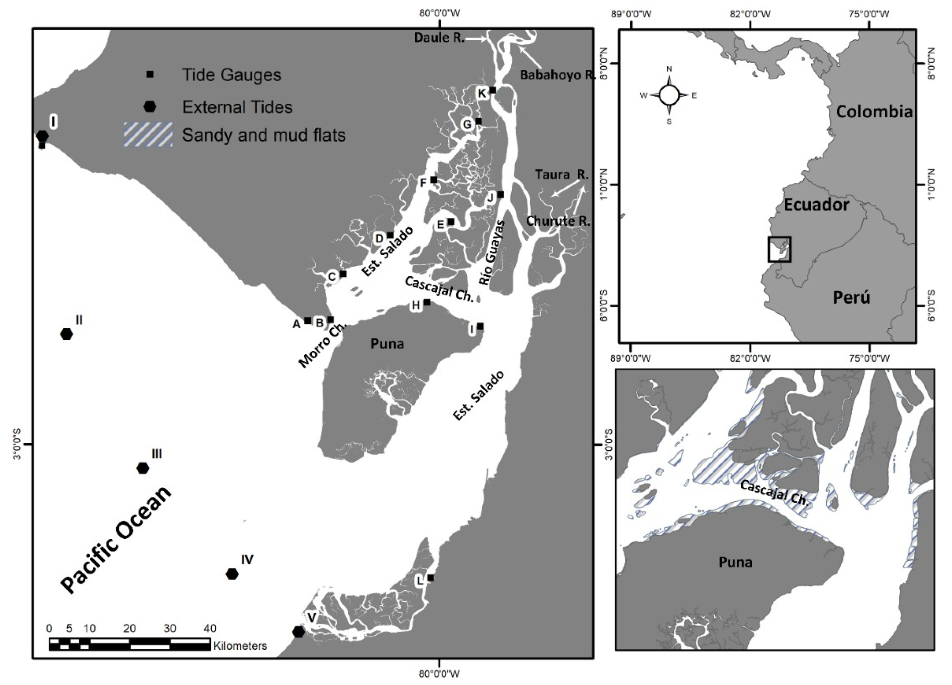
The Gulf of Guayaquil is naturally divided into an outer estuary and an inner estuary. The outer estuary originates near the western side of Puna Island (80°15′ W) and ends along the 81° W meridian, while the inner estuary extends from the tide mark of the Guayas River to the north coast of Puna Island [27,28]. Within the inner estuary, three sub-estuaries can be distinguished, although there are no defined limits among them: the Guayas River estuary, which is mainly influenced by the river of the same name; the Estero Salado, located on the west side, which lacks local freshwater sources and receives wastewater, mostly from the city of Guayaquil; and, to the east, the Churute estuary, which receives freshwater discharges from the Churute and Taura rivers [28], as shown in Figure 1.
The port of the Guayaquil city, located in the Estero Salado, is the most important port in Ecuador, and together with the port terminals situated in both the Guayas River and in the Estero Salado, manages approximately 80% of the non-oil dealer cargo nationally [29]. The design draft of the access channel to the maritime port is 7.5 m under any tide condition and 9.75 m during high tide. In the outer estuary, the tidal range varies from 1.5 m at neap tides to 2.3 m at spring tides. In the inner estuary, the amplitude increases gradually from 2.5 m to 3.6 m near the city of Guayaquil and the maritime port [30].
3. Methods
3.1. Hydrodynamic Modeling
To model the variation of the water level in the estuarine system, The Delft3D-Flow module of the open-source model Delft3D was used. The Delft3D-FLOW module solves the nonlinear three-dimensional (3D) or two-dimensional shallow water equations (averaged depth, 2DH). For this study, the 2DH formulation was utilized [23,31].
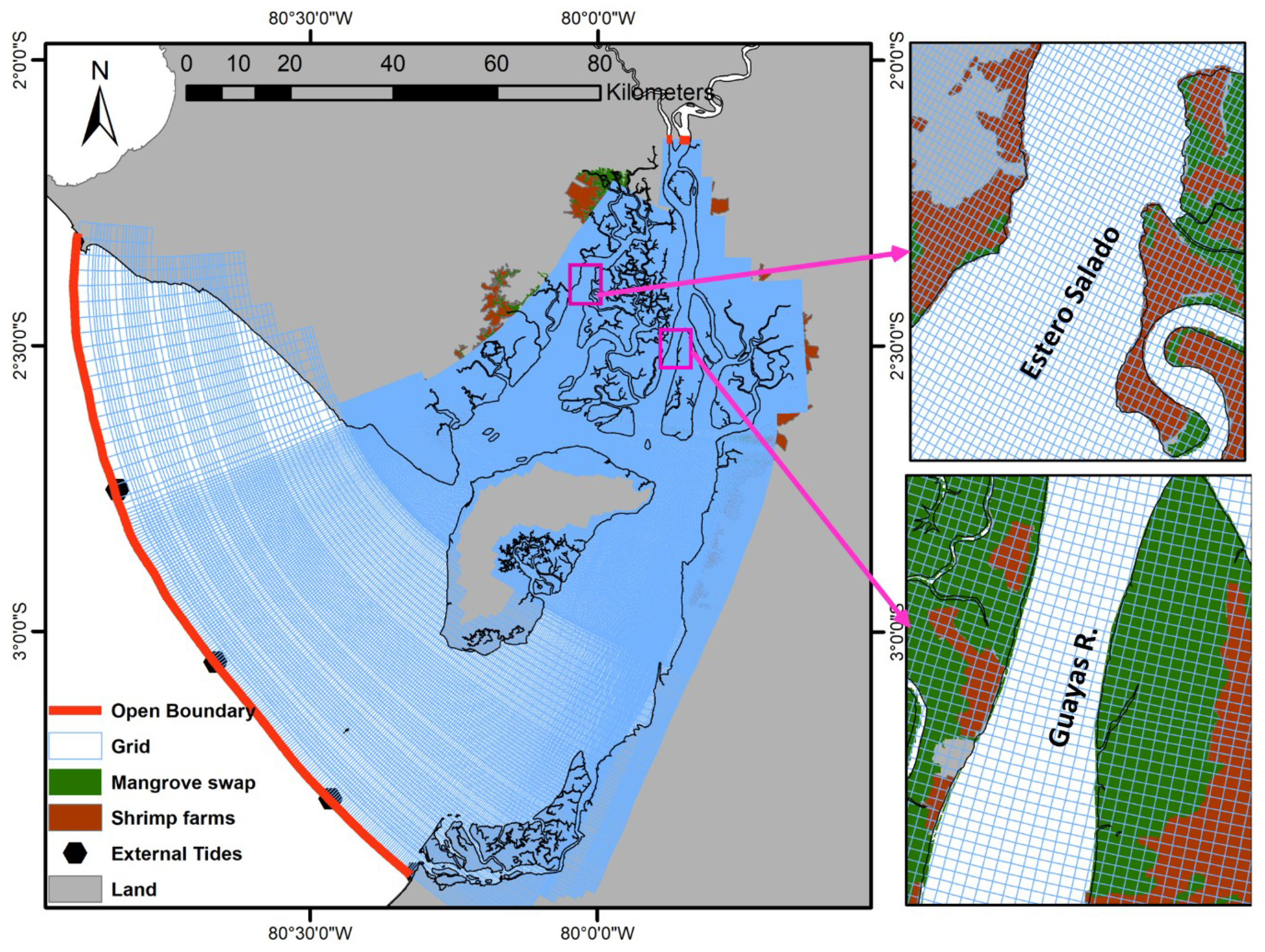
For the simulation, a structured mesh of 517 × 297 (153,549 nodes) was constructed. The cell size varied from 95 to 260 m in the inner estuary and from 260 to 3200 m in the outer estuary. This mesh covered both water bodies and mangrove zones. The model domain contained open boundaries at the seaward and landward ends. Landwards, the model has two open boundaries, which are the discharge areas of the Babahoyo and Daule rivers, as shown in Figure 2. The rivers’ discharge data were obtained from the hydrological information of the Meteorology and Hydrology Institute. The seaward boundary extension is 146 km. This boundary was subdivided into four segments of approximately equal lengths to analyze the behavior of the harmonic constants along the main channels in the study area. The tide information for these segments was obtained from the TPXO 7.2 global model [32].
The bathymetric surface in the inner estuary was obtained with the following surveys: two single-beam echosounder bathymetry surveys (SBES) carried out in the Estero Salado and Guayas River in 2009, at a scale of 1:5000; a SBES carried out in the small channels, located between Estero Salado and Guayas River, in 2005 at scale 1:4000; and several SBES carried out in the Jambelí channel between 2005 and 2014 at different scales. For the outer estuary, the bathymetry was compiled from some SBESs, nautical charts IOA 107 and 108, and SBESs collected by the US National Oceanic and Atmospheric Association. The land elevation was obtained from a combination of the SIG TIERRAS digital elevation model (DEM) and SRTM 1 arcsecond global elevation. The SIG TIERRAS DEM has a spatial resolution of 4 m2 [33]. Both bathymetric and land information were in reference to the mean sea level.
For the calibration of the hydrodynamic model, information from 12 TGSs from 1984 was used, as shown in Figure 1. These stations were installed by the Oceanographic Institute of the Navy as part of a project to study the causes of sedimentation in the navigation channel [30]. This year was chosen as it was the only period when water levels were measured throughout the entire estuarine system for one year, which allowed us to gain a clearer idea of the results of the model calibration. The 2009 information of the sea level elevation from the available TGSs was used to validate the model.
The time step selected for the simulations was 0.5 min. The parameters used in the model calibration are the bottom stress, represented in the Manning–Chezy formulation, and the horizontal eddy viscosity and diffusivity. In this calibration, a mesh with different values of eddy viscosity and diffusivity was used. To calculate the value of the eddy viscosity in each node mesh, the equation was used, where is the size length, is the typical speed, and K is a calibration constant, the range of which is from 0.05 to 0.15. The horizontal eddy diffusivity is calculated with: , where is the Schmidt number, the range of which is from 0.7 to 1.
Several simulations with a period of four months were performed, adjusting the Manning coefficient, calibration constant, and Schmidt number to optimize the adjustment between the model results and the observations of the sea surface level. The percentage variation of the root-mean-square error (%RMSE) (Equation (1)) and the Skill criterion (Equation (2)) were used to calibrate the model:
where are the observed and predicted water levels, respectively, is the number of observations made, and ΔR is the tide range. When the %RMSE is less than 5%, the calibration is considered excellent; when it is between 5–10%, it is considered very good [9].
Skill is based on the coincidence between the observed and modeled values, as shown in Equation (2). A Skill score equal to 1 corresponds to a perfect forecast; excellent, when Skill > 0.65; very good, 0.5 < Skill < 0.65; good, 0.20 < Skill < 0.5; poor, Skill < 0.2 [34,35]. The model is equal to the mean of the observations when the Skill score is 0 [9].
3.2. Tide Characterization of an Estuary
Tidal dynamics in an estuary are very complex. The analysis of the behavior of the main astronomical constituents along the estuary becomes fundamental to understanding the factor ruling its tidal dynamics. In this study, we follow a widely used approach to determine and analyze the amplitude and phase patterns of the main tidal constituents as well as the form factor and dominance type [9,36,37]. For this analysis, the semidiurnal harmonics M2, N2, and S2, which are the most energetic both in the continent and estuaries (they contain approximately 75% of the tidal signal) [36], were chosen. The diurnal constituents K1 and O1 and the overtide constituents M4 and M6 were also selected for this study [38]. The analysis of these constituents allows us to determine several important indicators of the tide, such as form factor, tide asymmetry, and ebb/flood dominance.
3.2.1. Analysis of the Harmonic Constituents in the Tide Gauge Stations and Each Mesh Node of the Hydrodynamic Model
The variation of the tide height can be expressed as follows [39] (Equation (3)):
where is the water level at time (t); is the mean sea level over a certain time period; m is the number of constituents; is the nodal amplitude factor; is the local tidal amplitude of a constituent; is the frequency of the constituent j; are nodal and Greenwich arguments for tidal constituent j; is the epoch (phase lag) of tidal constituent j relative to the moon’s transit over the tide station; and B = is the change of the water level induced by other dynamic factors [7,37].
The tide gauge records of the year 1984 were used in order to calculate the harmonics in the TGSs. In the mesh nodes for harmonics analysis, the sea surface elevation obtained from four months of simulation was used. This period of time was selected since for harmonic analysis, the minimum observation span considered is the hourly height readings over one lunar month, i.e., about 29.5 days [18].
The amplitude and phase values of the harmonic constituents of both the gauge stations and the nodes in the grid were calculated with the software T_tide [40], which is based on a classical tidal harmonic analysis method [17]. The main harmonics of the observed data and model results were compared [9].
3.2.2. Form Factor
The form factor (F) was used to determine the type of tide in the estuarine system. It is defined as the ratio between the diurnal constituents (K1, O1) and semidiurnal constituents (M2, S2) (Equation (4)):
3.2.3. Tide Asymmetry
The asymmetry of the tide is often described by the difference or relationship between the duration of the rising tide (flow) and the descending tide (ebb). If the flood period is shorter, the asymmetry of the vertical tide is flood-dominant. If the ebb period is shorter, the asymmetry is ebb-dominant. The reasoning behind this is that a shorter flood duration implies stronger flood velocities (peak) and therefore higher transport rates in the flood direction, or vice versa [42].
The asymmetry of the tide is induced by the nonlinear propagation mechanism of the tide [9]. Asymmetry is commonly described as the distortion of the tidal wave. The dominant constituent is M2, and M4 is the main constituent of the harmonic M2 and is mainly generated by nonlinear interactions [38]. The nonlinear transfer of energy by friction, continuity, and advection intensifies M4 and other overtides. The constituent M4, along with other harmonics of a higher order, is responsible for the distortion of the tidal wave. M4 has also been found to be the main contributor to the distortion of tides in coastal areas [43].
A comparison of the constituent M4 and the constituent M2 can be used as an indicator of the degree of distortion and asymmetry of the tides. The degree of distortion caused by the constituent M6 must also be considered, because M6 is important in the bottom friction effects analysis [9]. Friedrichs and Aubrey [43] proposed Equations (5) and (6) to describe the tide:
where is the amplitude ratio; > 0.01 indicates a significant distortion in the tide wave.
where shows the phase. For both and , if , the flow is flood-dominant. If the flow is ebb-dominant. This relationship is an indicator of sediment transport. If the estuary is flood-dominant, the transport of sediment is towards the interior of the estuary. In contrast, if the estuary is ebb-dominant, sediment tends to be transported out of the estuary.
3.3. Chart Datum Determination
The CD is the plane of reference to which soundings and drying heights on a chart are referred. It is usually taken to correspond to a low water stage of the tide [44]. Each country has its own level of reduction. In the case of Ecuador, the MLWS is the CD used. The MLWS is the average height of the low waters of spring tides during a time period [45].
A one-year water level prediction was carried out with the values of the harmonics, both in the gauge stations and in the mesh nodes of the hydrodynamic model. The T_tide software was used for these predictions. The CD in each tide gauge station, as well as for each of the nodes of the grid, was calculated using Equation (7):
where is the low water at the time of spring tide , and is the number of low water tides at the time of spring tide over a period of one year. The information of the CD in each node of the mesh was interpolated using the inverse distance weighting (IDW) method. A 2D surface of the CD was obtained.
Hydrodynamic models are very sensitive to bathymetric information [46]. For this reason, even though a suitable calibration of the hydrodynamic model is reached, the magnitudes of the CD could be underrepresented or overrepresented when contrasted with the CD of the tide gauges. The offset of the CD was calculated by subtracting the value of the CD in the tide gauge from the modeled CD. The values of the offsets were spatially interpolated through the entire mesh using the tension spline method. These corrections were then added to the original CD surface so as to provide a more accurate representation of the CD:
where is the final CD surface; is the original CD surface, computed using the data obtained from the hydrodynamic model; and are the modeled offsets. This surface was validated with TGSs located in both the Estero Salado and Guayas River. These stations were not used in the determination of the surface corrector.
3.4. Assessment of the Tide Correction Methods
In the hydrographic surveys, the charted depth or reduced depth (D) is calculated by taking four components into consideration, as shown in Equation (9):
D = OD − H + dyn_draft − WL
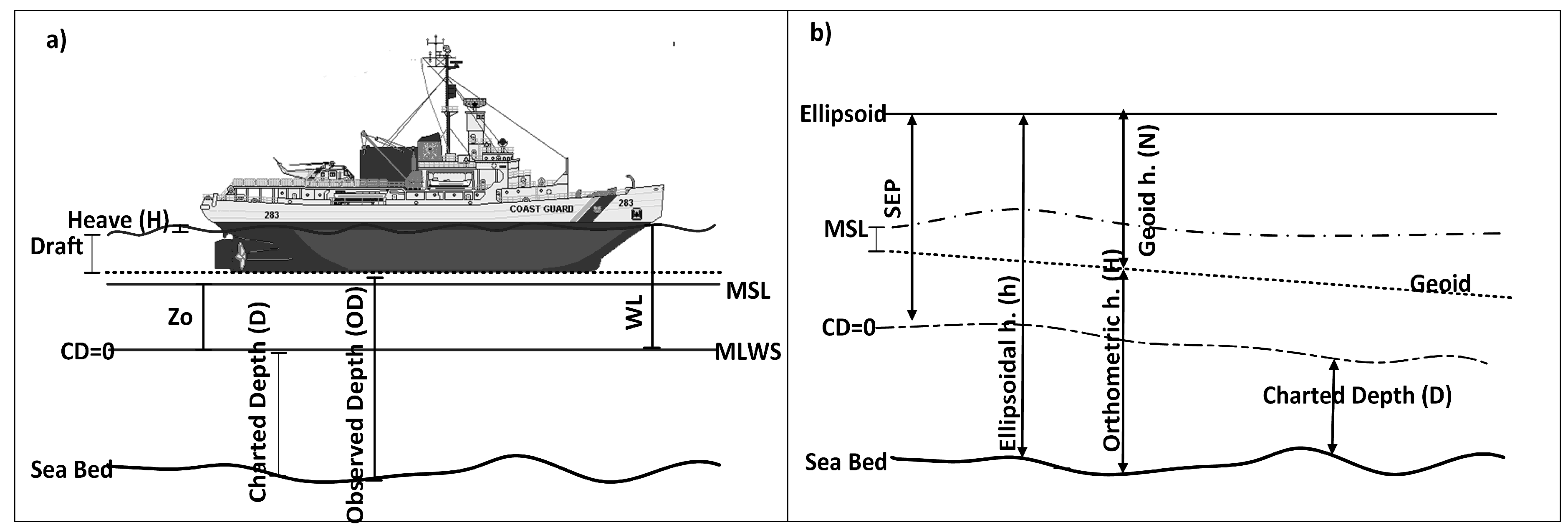
The observer depth (OD) is obtained by measuring the echo-sounder, to which a series of corrections are made; the dynamic draft (dyn_draft) considers the squat, draft, and load variation; heave (H) considers the vertical movement of the vessel; and the water level (WL) represents the water height over the CD, as shown in Figure 3a.
The uncertainty associated with the charted depth is calculated by the law of propagation of variance, combining the individual variance of each component [47] (Equation (10)):
where is the total variance associated with the observed depth, is the total dynamic draft uncertainty, is the total variance of the heave, and is the total variance associated with the water level. The uncertainty value of the CD is a subcomponent of the . The International Hydrographic Office (IHO) [48] and NOS [49] manuals establish that the allowable error contribution for tides and water levels to the total survey error budget typically falls between 0.20 m and 0.45 m. The total error of the tides and water levels can be considered to have component errors of: (a) the measurement error, which should not exceed 0.10 m at the 95% confidence level; (b) the error in the computation of first reduction tidal datums and for the adjustment to 19-year periods for short-term stations; and (c) the error in the application of tidal zoning. Estimates for typical errors associated with tidal zoning are 0.20 m at the 95% confidence level. However, errors for this component can exceed 0.20 m if tidal characteristics are very complex.
One of the main challenges in hydrographic survey planning in an extensive and complex estuarine area is to determine the places where the principal and secondary tide gauges should be installed in order to reduce the water level uncertainty. In a hydrographic survey, the number of TGSs will depend on the tide correction method selected.
For the tidal zoning method, the number of TGSs is linked to the shape of the CD. If the CD shape is too complex, more tide gauges will be needed to reduce the uncertainty. However, in most cases, due to logistical limitations, not enough TGSs can be installed to provide direct control over all areas of a hydrographic survey [16]. Standard procedures for determining how far one tide station should be installed from the other in an estuary have not been developed. However, some hydrographic services have established an empirical specification based on the maximum variation of the CD between zones. For instance, the Directorate of Hydrography and Navigation has established the maximum difference between zones as 0.10 m [50].
In this study, the approach to reconstruct the river flow and determine the number of scenarios [51] was adapted to define the number of tidal zones in the estuaries. The CD profile of the navigable channels was extracted from the final CD surface. The CD values of the profile were grouped into n groups of CDs in order to reconstruct the profile. The higher the numbers of the groups, the more similar the reconstructed CD profile to the original profile. Thus, it is important to select a minimum number of CD groups. In this assessment, the evaluation of the correlation between the original CD profile and the reconstructed CD is proposed using the %RMSE as it is defined in Equation (1). The similarity between the original and the reconstructed CD can be qualified as good if %RMSE has a value between 5–10% and excellent for an %RMSE lower than 5%. Since, in the study area, at least a first-order hydrographic survey is required, a %RMSE value of 5% was selected.
The ERS method uses high-accuracy vertical GNSS and transformation models to replace traditional tidal correctors [16,52]. This method requires the definition of three models: ellipsoid, CD, and geoid, as shown in Figure 3b. The key aspects of this method are to determine the CD to geoid separation (N) and the height of the CD above the ellipsoid reference, i.e., separation surface (SEP) [52,53]. Figure 3b represents the three surfaces and the separation between the surfaces.
For small survey areas, a single value of the geoid/ellipsoid (N) separation and SEP, calculated at a tidal benchmark, could be sufficient. When working in a large survey area or areas with complex tides, one cannot treat the SEP as a constant, since the CD to geoid models become more complex [52]. To use ERS in these types of areas, Mills and Dodd [16] suggest three methods: the first method uses SEP observations at multiple locations around the survey area and interpolates between them; the second looks at a refinement of the first method, where the interpolation of the SEP between gauge locations is performed using a geoid model. The third method establishes the use of a hydrodynamic model to compute the different tidal data. In this study, the first and third methods will be assessed. To analyze the first method, CD surfaces will be constructed by interpolating the CD values obtained from both the tide stations and the tide points of the open contour condition using the IDW and tension spline (TPL) interpolation methods. The CD profile of the navigable channels will be extracted from these surfaces. The similarity level between these profiles and the profiles obtained with the CDF will be calculated using the %RMSE criteria.
3.5. Chart Datum in Different Scenarios
In addition to helping us solve the problem of CD, the hydrodynamic models help us to evaluate flooding events, coastal ecosystem responses to sea level rise, marine boundaries [25], and the impact of anthropogenic action in the aquatic habitats [54]. Some of these factors also affect the surface of the CD. In this study, two scenarios produced by the actions of human activities will be analyzed.
Scenario 1: Climate change represents a hazard to Guayaquil City, located in the north of the study area. Several solutions have been proposed for preparing Guayaquil against floods, which might occur in the future [55]. One of the solutions considered was the construction of a barrier in the Guayas River to reduce water levels and salt intrusion [55]. The effect that this barrier has on the CD surface will be evaluated.
Scenario 2: Mangrove trees could be present in tropical estuaries. The roughness of mangrove trees is much greater than that of mudflats and marshes [56]. An increased roughness coefficient of the riverbed reduces flow velocity and raises water surface levels [57]. Thus, the coverage alteration of the mangrove forest affects the CD surface. In the study area, the expansion of shrimp farms and city sprawl has led to the loss of 24% of mangrove coverage [58]. In this study, we will compute the effect in the CD if the mangrove coverage is removed from the estuarine system.
4. Results and Analysis
4.1. Simulation and Calibration of the Hydrodynamic Model
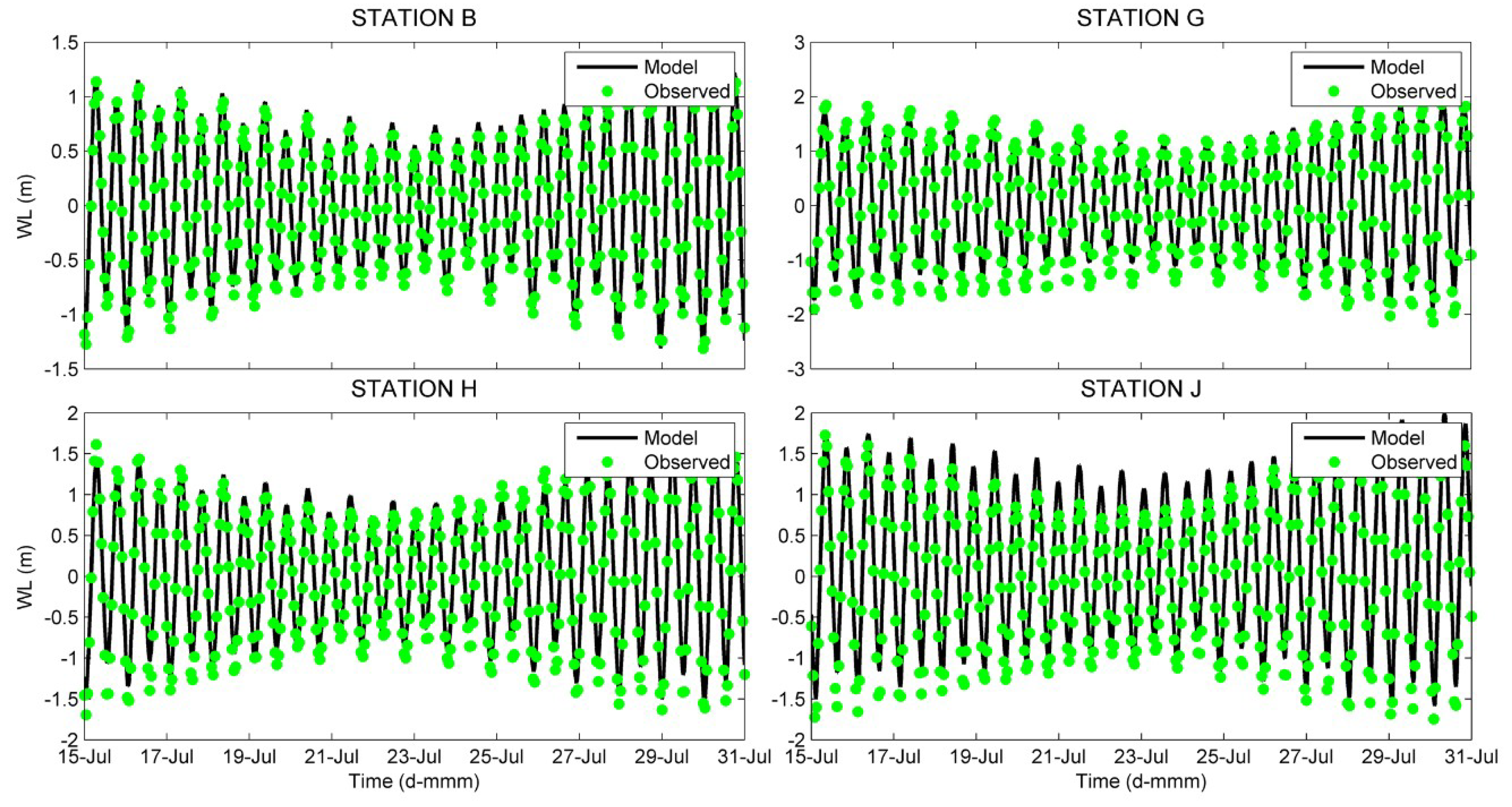
The best model results were achieved with a calibration constant and Schmidt number of 0.05 and 0.7, respectively. The Manning coefficient value selected for the mangrove swamp was 0.15, 0.0205 for the Estero Salado and Cascajal Channel, and 0.0195 for the Guayas River. The simulated water surface fluctuations at the four stations (B, G, H, and J) are compared with the observed data, as shown in Figure 4.
Table 1 shows the final calibration and validation values of both the %RMSE and the Skill score. Both parameters range between excellent and very good, which indicates that the model adequately simulates the sea level.
4.2. Harmonic Constituent Analysis
Figure 5 shows the amplitude values of the main harmonic components calculated with the observed (square) and modeled (circle) time series. The stations located in the Estero Salado (B, C, D, F, and G), as well as those situated in the Guayas River (I, J, and K), show values of the constituents that are quite similar.
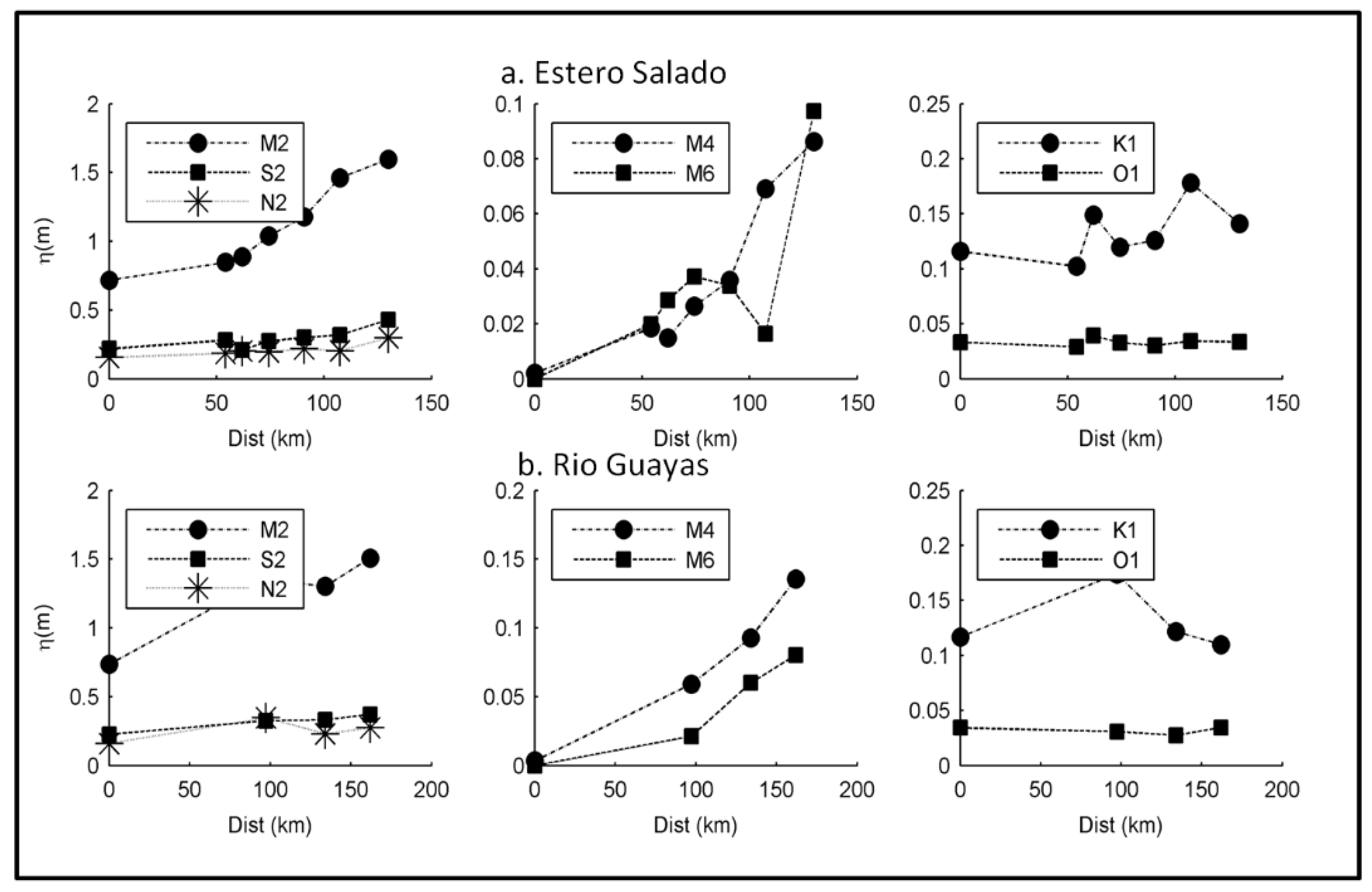
In Figure 6a, the behavior of the main constituents along the estuarine system can be observed. In the Estero Salado, the amplitude of M2 increases considerably from its mouth (at kilometer 50), while N2 and S2 increase gradually. The semidiurnal harmonics increase as the tidal wave enters the estuary, and the percentage increase of M2 is 82%. The amplitude of the overtide M4 decreases slightly, after the entrance of the tidal wave into the estuary, and later increases. M6 has a greater amplitude than M4 from the mouth of the estuary until approximately km 80, where it suddenly falls and then increases quickly. The generation of M4 is essentially due to the nonlinear effects in the continuity equation and the depth effect on the bottom friction, while M6 is mainly forced by bottom friction [9,59]. Figure 6a suggests that bottom friction is dominant from the mouth of the Estero Salado to the D station. The diurnal constituents show a slight growth from the mouth of the Estero Salado.
In the Guayas River (Figure 6b), the semidiurnal harmonics M2 and S2 increase from the shelf towards the interior of the river. Harmonic N2 has its maximum value near km 100 and then decreases. The M4 and M6 harmonics increase towards the interior of the Guayas River. The diurnal K1 harmonic has its maximum value near 100 km.
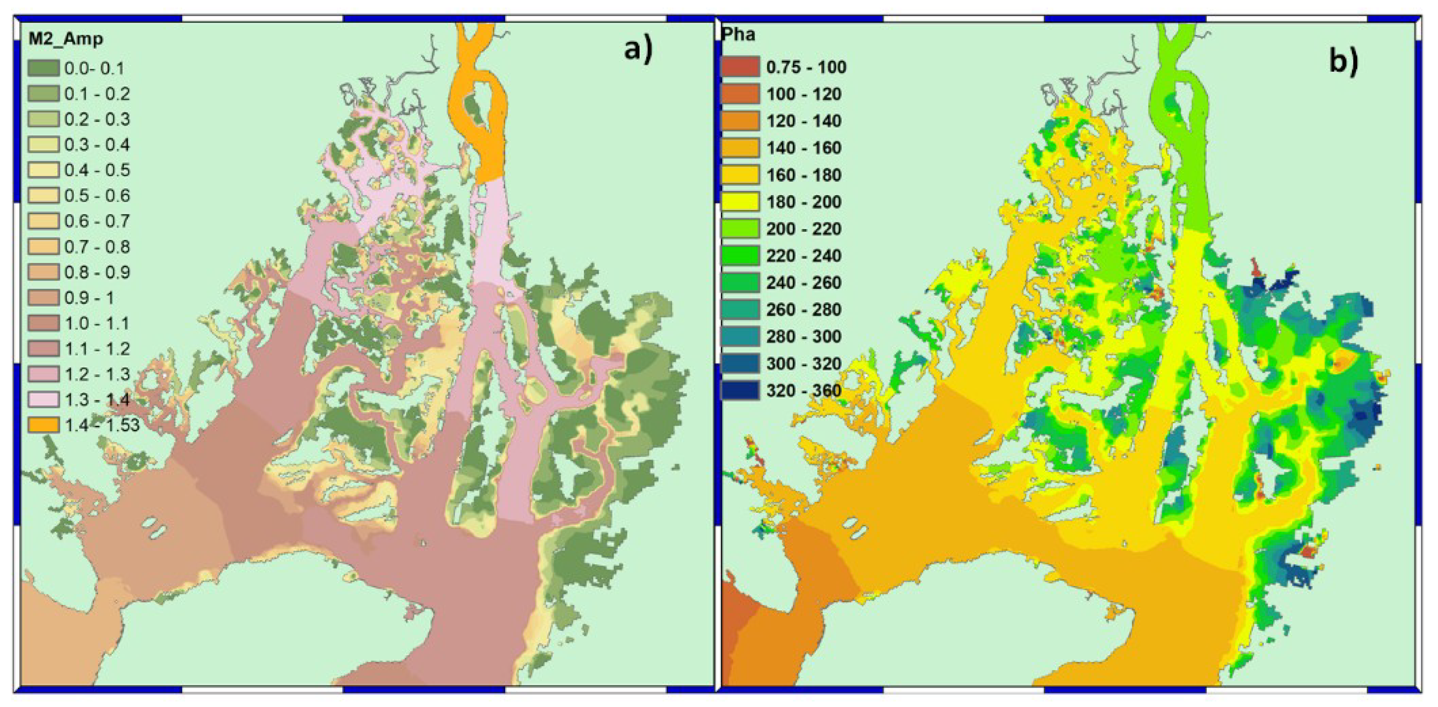
Both the amplification and damping of the tide in an estuary depend on the convergence of the banks and friction. If the effect of the convergence is greater than that of the friction, the tidal wave will be amplified. When the friction is greater than the convergence effect, the wave is attenuated [22,60]. Figure 7a, shows the harmonic M2 increase in magnitude along all the channels and shows a reduction in the mangrove area and in the shoal areas of the Cascajal Channel. This means that in the channel zones, the effect of convergence is more important, while in the mangrove zone, the effect of friction is greater.
In Figure 7b, it is observed how the phase of the harmonic M2 is strongly modified, which causes the propagation of the tidal wave to be delayed upstream due to the convergent morphology of the estuarine system and the variation of the water depth. These factors produce variations in the bottom friction, inducing a reduction in the propagation speed of the tide. In Figure 7b, it is observed that the phase near the entrance to the Estero Salado is ~130°, and in station G, it is ~175°, which means that the delay of the harmonic wave M2 is 1 h 33 min (~45°). This value is smaller than the delay of the tidal wave, which is 2 h 25 min.
4.3. Tide Characterization in the Estuarine System
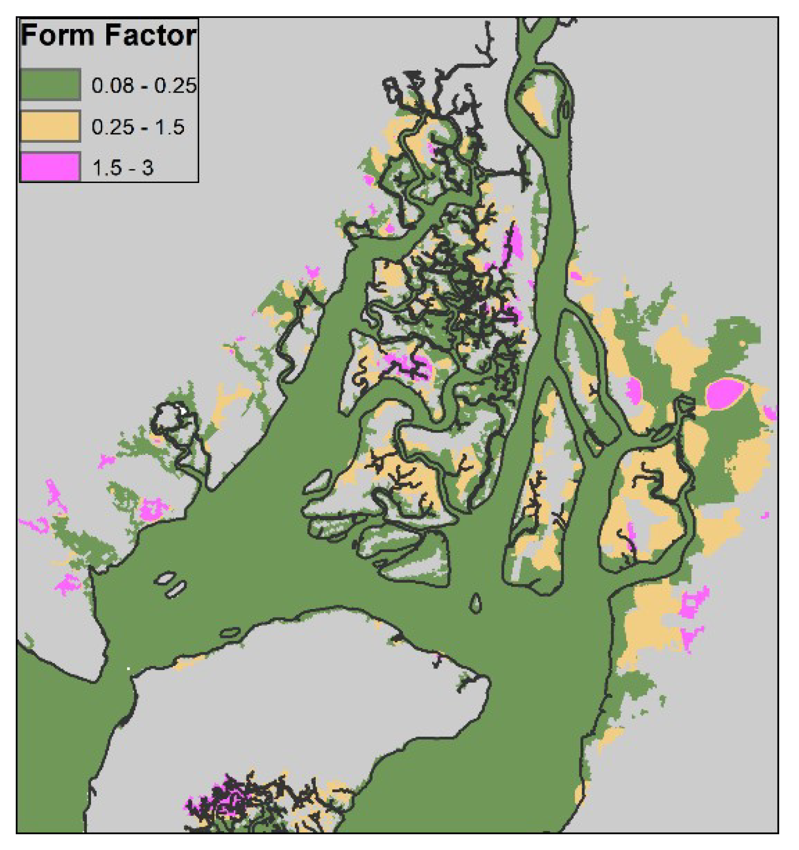
The form factor was calculated in each node of the mesh. The main and secondary channels have a semidiurnal tide, while in the mangrove area, zones with semidiurnal and mixed tides were found, as shown in Figure 8.
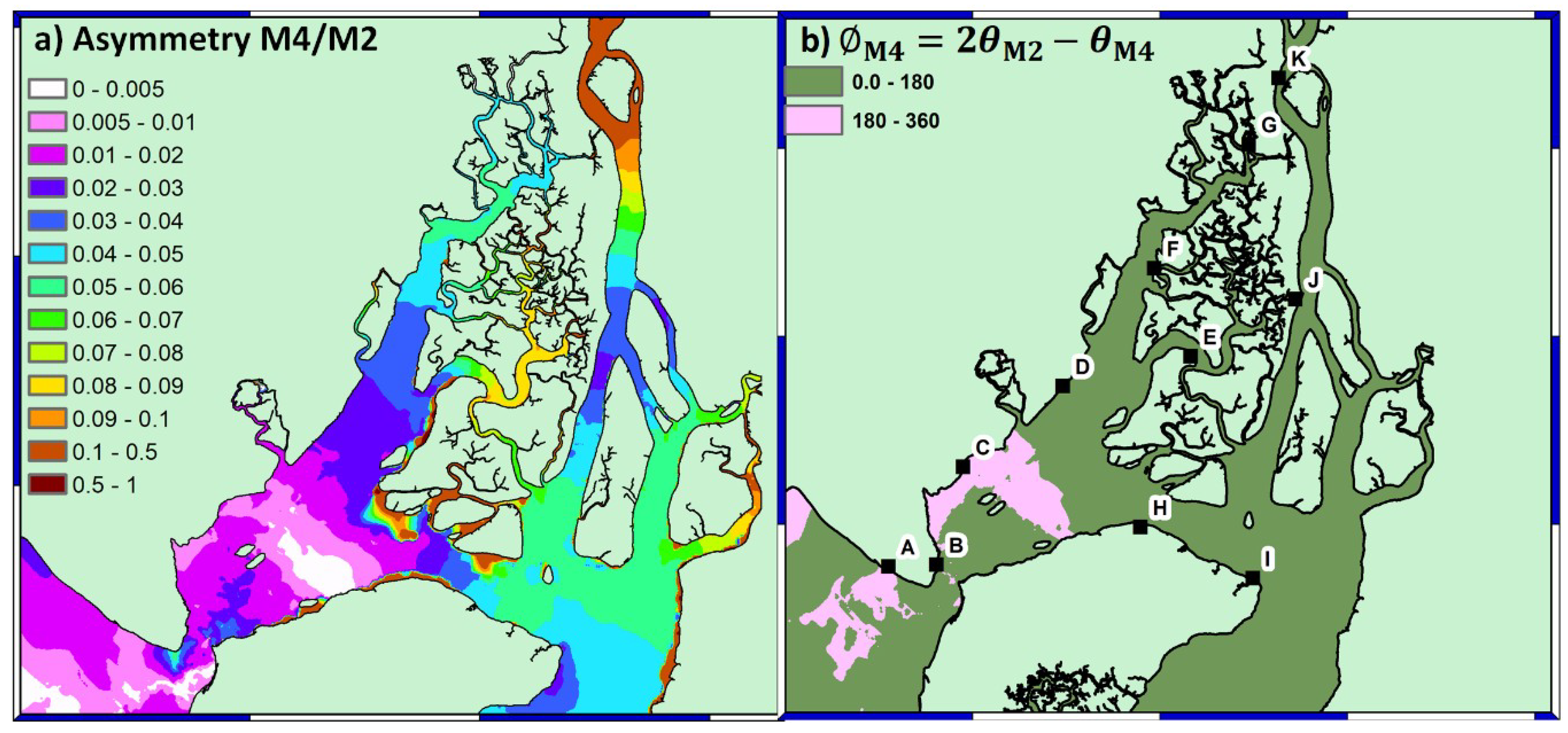
From Figure 9a, it can be seen that the Guayas River has higher values of asymmetry than the Estero Salado. The asymmetry difference indicates that the bed of the river has greater dynamics than the bed of the Estero Salado. From the analysis carried out in each TGS, it was determined that, except for stations A and G, the stations show a flow-dominant estuarine system. Figure 9b shows the analysis of the estuary type using the phase values of the harmonic constituents obtained in each node of the mesh. It is observed that the estuary system is mainly flood-dominant, which means that sedimentation mostly occurs towards the interior of the system. The ∅ values of stations C and G do not coincide with the analysis conducted at each tide gauge station.
Both the flood type and tidal asymmetry of an estuary have an effect on the navigability, due to their influence on the processes of erosion and accretion of the seabed. This has a direct consequence for the determination of both the critical depth [9,43] and the periodicity of hydrographic surveys.
In this case study, the results of the flood type and tidal asymmetry show that the Guayas River would present the most significant sedimentation problems. Therefore, hydrographic surveys should be carried out more frequently in this water body, with greater detail in the observations of sea level. Therefore, both asymmetry and type of flow could be used as new factors to estimate hydrographic risk [61].
4.4. Chart Datum Surface
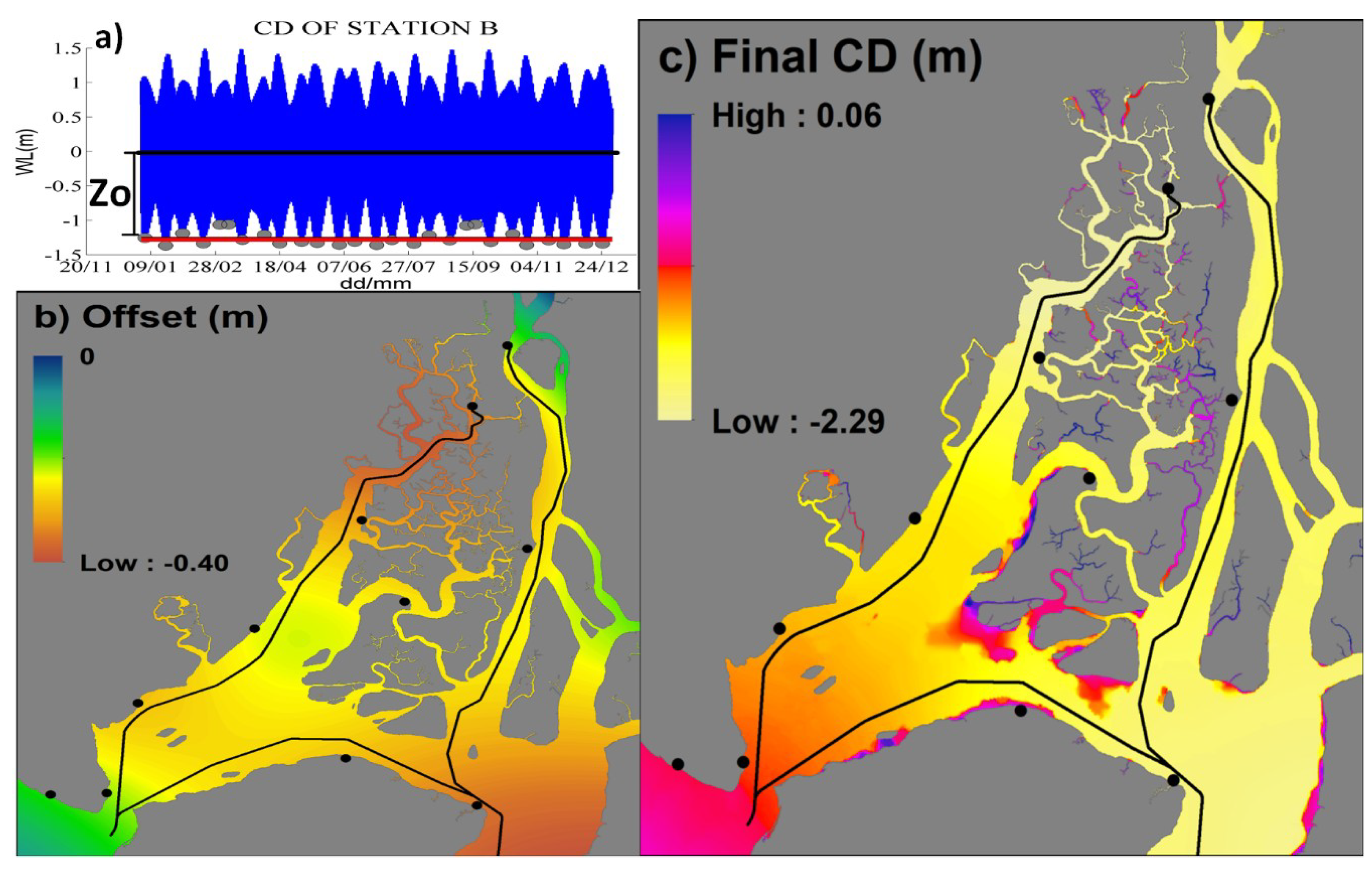
In Figure 10a, the gray circles indicate the lowest low water during each spring period in a year, while the solid black line represents the MLWS or the CD for station B. This value is not constant along the estuary due to the convergence, which amplifies the tidal wave, so the location of the CD changes in each tide station.
Table 2 shows the difference between the modeled CD surface and the CD of the tide gauges. The mean value of the CD offset is −0.204, and the standard deviation is 0.11. In the outer estuary (station A), the model calculates the vertical position of the CD accurately. In the inner estuary, the model underestimates the CD surface at all stations. The TGS offset grows from the inlet to the upper estuary in the Estero Salado. In the Guayas River, the offset values are similar.
There was some uncertainty regarding the data recorded at station E. For this reason, this station was not used to generate the offset surface in order to correct the original CD surface. Figure 10b shows the offset surface, and Figure 10c shows the CDF surface. The tension spline method generates a surface with offset values that make the surface pass exactly through the control points. Two temporal stations installed in 2009 were used to validate this surface.
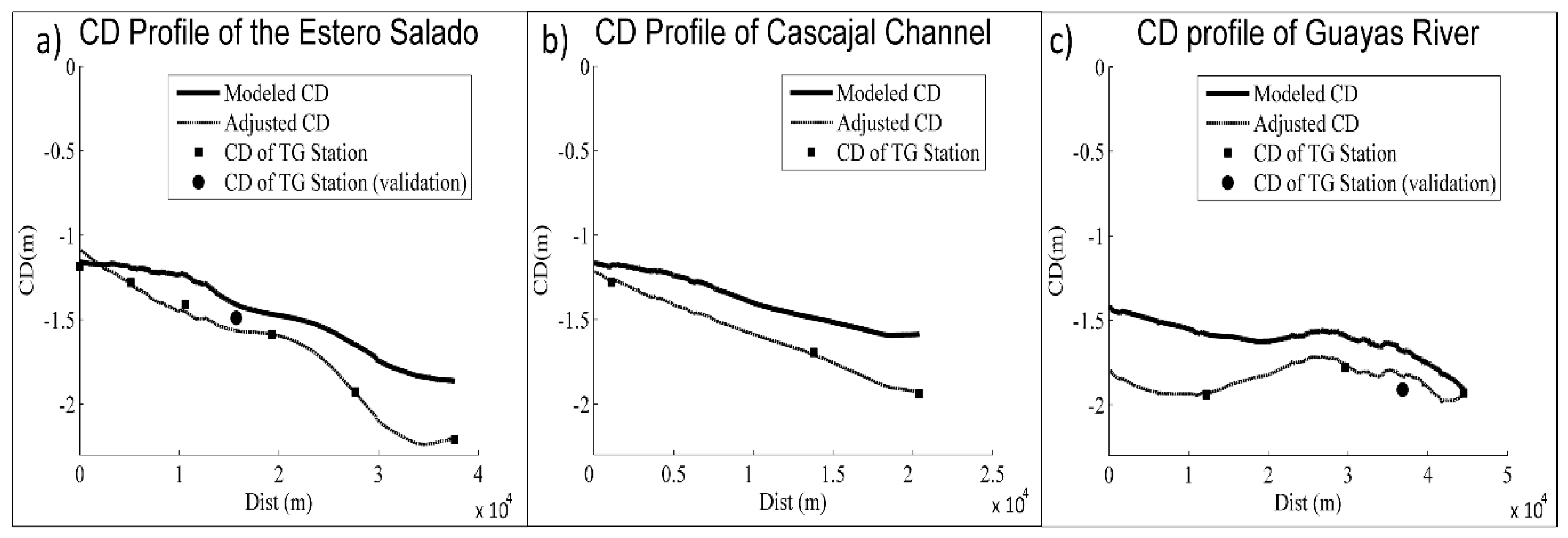
Both the modeled CD profile and the adjusted CD profile along the navigable channel in the Estero Salado, Cascajal Channel, and Guayas River are shown in Figure 11a–c. The black square represents the values of the CD obtained in the tide gauge station used to generate the offset surface and to calibrate the model. The black circles in Figure 11a,c represent the CD of the tide gauge used to validate the model. The difference in the CDs of these two TGSs with the adjusted CDF surface was ~7 cm.
It can be noted that the CD has neither a straight slope shape nor a zoning form. The real CD shape is a slightly negative slope with an undulating surface, due to the combined effect of the friction and the convergence that amplifies the tide.
4.5. Assessment of the Tide Reduction Methods
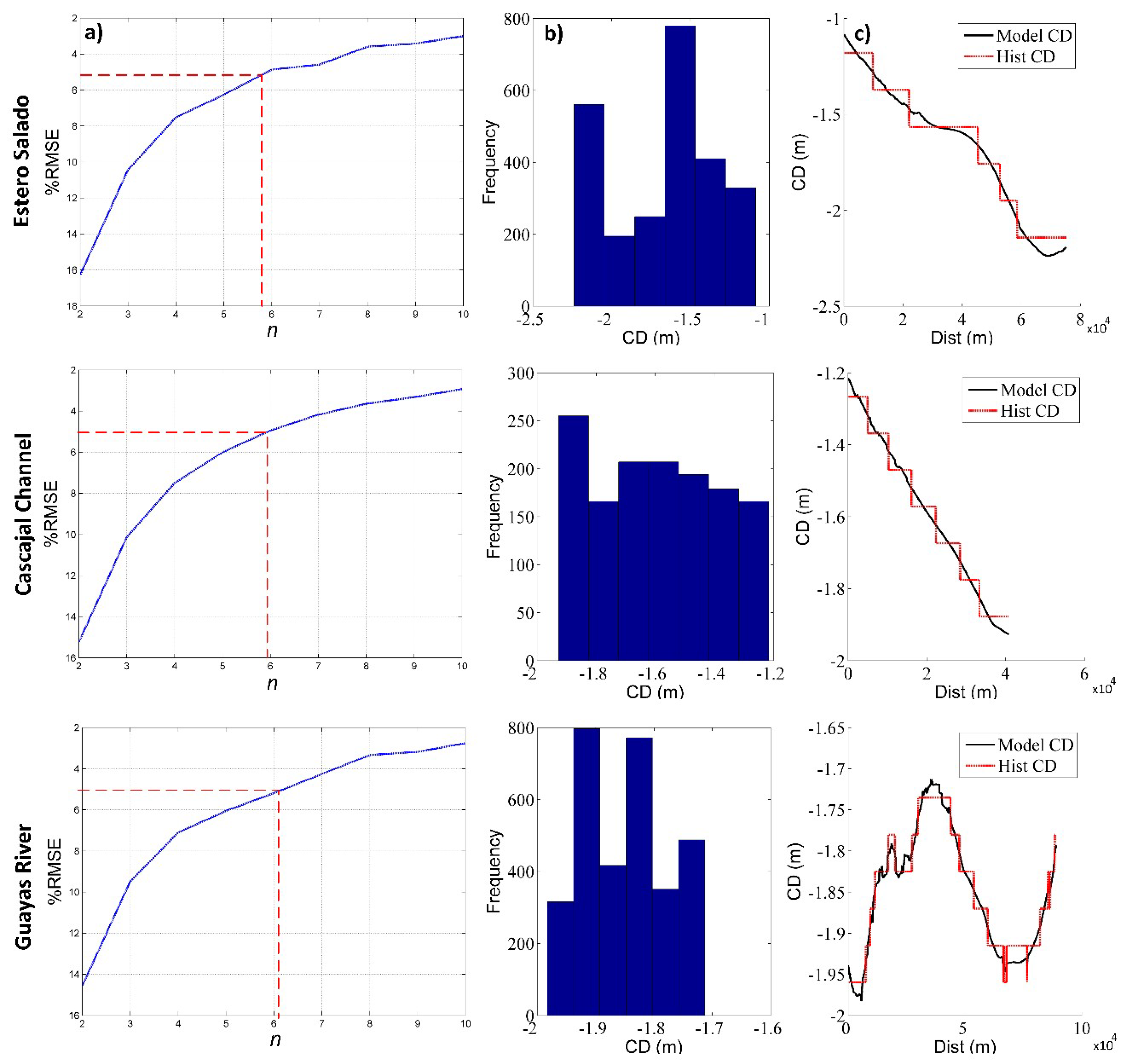
Through an iterative process, the value of n ~6 in the three water bodies was determined, as shown in Figure 12a. The bin width (Figure 12b) gives us the difference value between tidal zones. Due to the complexity of this estuarine system, three separation values between tidal zones have been found: Estero Salado = 0.19 m; Cascajal Channel = 0.11 m; and Guayas River = 0.049 m.
If the separation value determined for the Estero Salado were selected for the entire estuarine system, the shape of the CD in the other two bodies of water would not be reproduced adequately, and errors would therefore be introduced into the final depths. If the value determined for the Guayas River were selected for the entire estuarine system, an excessive number of tidal zones in the Estero Salado and Cascajal Channel would be established. Thus, the hydrographic survey will require an excessive logistical effort.
Using the tidal zoning method, the Estero Salado and Cascajal Channel will require six tidal zones, while the Guayas River will require ~14 tidal zones, as shown in Figure 11c. For this reason, the establishment of tidal zones for hydrographic surveys of special and first orders is not very suitable for areas with complex tidal characteristics, due to the logistical effort that is required to install a network of tide gauges allowing for the proper reconstruction of the CD. Therefore, it would be convenient to consider the use of ERS for this type of environment.
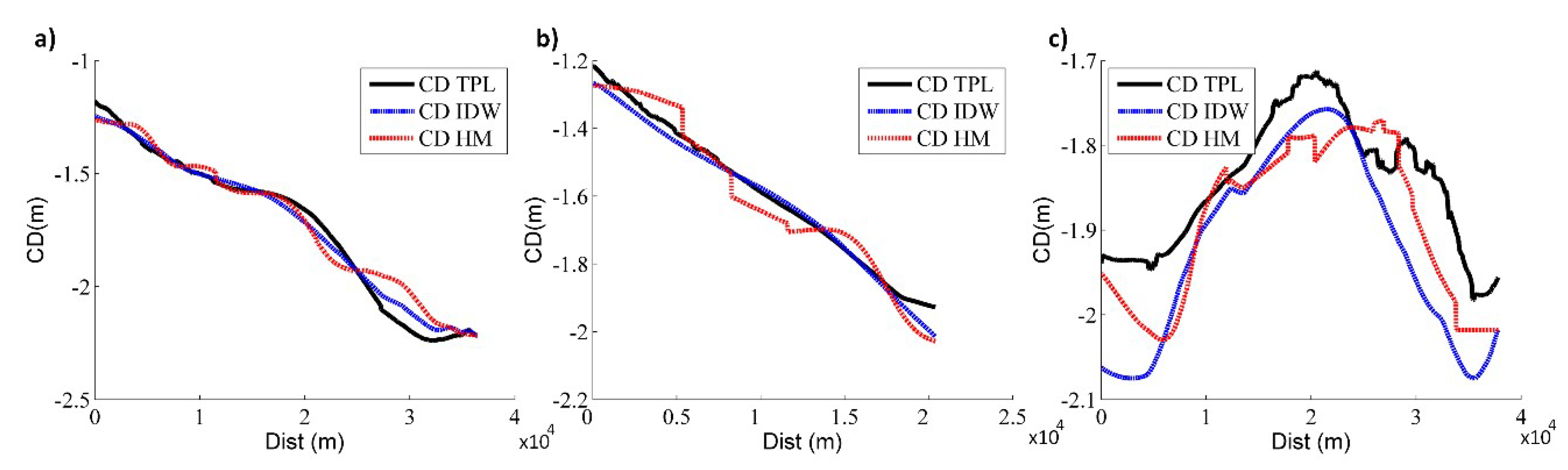
In order to use the ERS method, once the CD model is complete, it must be attached to the ellipsoid. In order to do this, GNSS data must be collected at tide station sites to determine the separation between the CD and ellipsoid. Additionally, the difference between ellipsoid and geoid must be determined, and then that between geoid and mean sea level, which is the reference level of the hydrodynamic model. If a hydrodynamic model is not available, to solve the SEP problem, the CD can be calculated by the interpolation from the CD of the different tidal gauge stations. Figure 13a–c shows the CD profiles calculated from both the hydrodynamic model and interpolation with the IDW and TPL methods.
Taking as a reference the CD calculated with the hydrodynamic model, Table 3 shows the differences between the CD profiles. The %RMSE values of the CD profiles obtained with the IDW and TPL interpolation methods are close to 5%, so it can be established that in these channels. The interpolation methods give a good level of reliability. However, in the Guayas River, the %RMSE increases to 23–33%, with a maximum difference between the surfaces of 11–17 cm, reducing the level of reliability.
In regions with complicated hydrodynamics, the use of hydrodynamic models to solve the SEP problem for an ERS survey is appropriate to reduce vertical uncertainty. The use of interpolation methods is an option that must be evaluated in each specific place. Once a suitable CD model is determined, tide stations will only be required as a backup for quality control and redundancy.
4.6. Evaluation of the CD in Different Scenarios
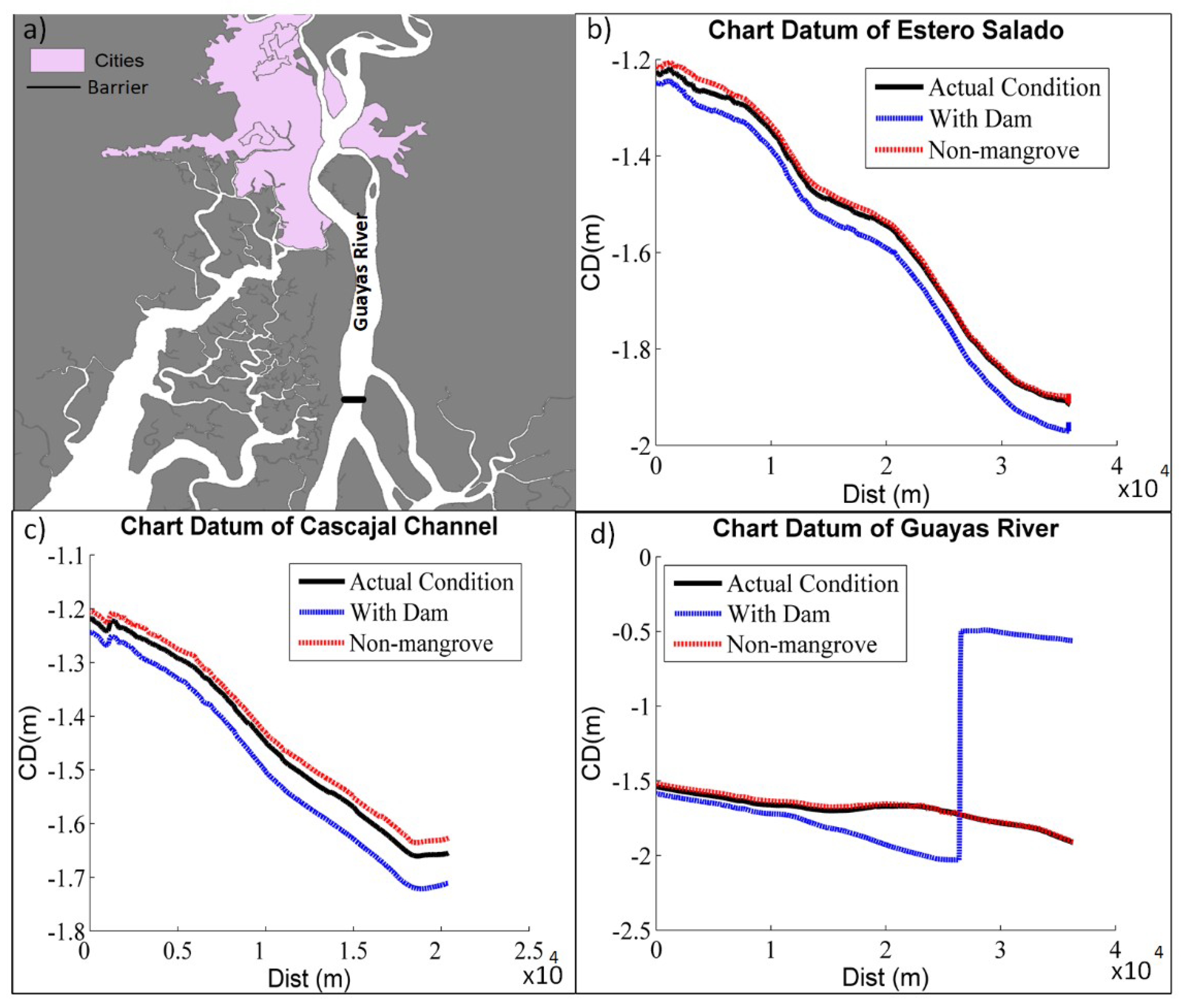
Figure 14 shows the profiles of the navigation channels in the current situation and the two scenarios, and Table 4 indicates the variation, in meters, between the current situation and both scenarios.
In Scenario 1, the barrier is situated downstream of Guayaquil City, at location A, as shown in Figure 14a. The CD has a different behavior upstream of the barrier than in the rest of the estuary (Figure 14b–d). Upstream, the CD rises to an average of 1.2802 m and the tide levels decrease substantially. Below the barrier, the reflection effect produced by the barrier is observed [8,9]. The CD initially has a considerable deepening of around 0.33 m and then reduces to 0.14 m in the rest of the estuary. This scenario could have both favorable and unfavorable effects on navigation in the study area, as some of the ships that navigate these channels require the benefit of the tide to pass through critical areas. In the channels located in the Estero Salado and Cascajal Channel, navigation will benefit from the effect of the barrier, while navigation in the Guayas River will be severely affected, since one of the critical areas is located upstream of the barrier, where the CD rises and the tide levels are reduced.
In Scenario 2, when the mangroves are removed from the study area, the profiles of the CD rise along the entire estuarine system (Figure 14b–d), which means that in this scenario, the water levels tend to decrease. The range of the average variation of the CD in the three channels is from 0.0279 to 0.0111 m. Therefore, the withdrawal of mangrove coverage will have little effect on the CD.
The main use of the CD is in the navigation. Hydrodynamic models allow us to build a local or global continuous and seamless CD surface. This information is used to reduce the uncertainty of a hydrographic survey and produce a better bathymetric surface such us the navigation surface. Besides, the CD surface from hydrodynamic models can be used to improve the safety of navigation. The variation of the vertical position of the CD can be used as an indicator of the anthropogenic action in the navigation. If the CD goes upward, the tide levels are reduced, and vice versa.
Another main use is the international maritime boundary delimitation. The internal waters, territorial waters, and maritime zones are measured from the baselines. The base line can be normal, straight, or a combination of both. The baseline corresponds to low water [62]. The precise definition of the chart datum is crucial to define the low water line. The accuracy of the vertical datum depends on the length of the tidal records and the remoteness of the area to be delimited from the tide gauge stations [45]. Once the CD is calculated in the study area, either a geodetic/topographic or bathymetric survey could be used to calculate the low water for both straight and normal baselines.
The determination of the baseline has two main problems. First, some places are of difficult access. Therefore, both geodetic and bathymetric surveys cannot be carried out. Second, adjacent or opposite states may use different levels to establish their baselines; this could produce discontinuities [45].
The use of hydrodynamic models to establish the CD helps us to solve these problems. A suitable high-resolution grid along the coast can be used to determine the CD at each node of the grid. The baseline can be calculated by interpolating this information. We can produce both nationally and internationally seamless CD surfaces that would facilitate more effective sharing of vertical data to resolve problems of marine cadasters and claims to sovereignty [17].
5. Sources of Uncertainty in the Hydrodynamic Model
Hydrodynamic models have numerous sources of uncertainty. One of the main sources of uncertainty is the bathymetric information. Cea and Frech [46] showed that the calibration that incorporates bathymetric uncertainty could be significantly more efficient than a classic calibration based only on the adjustment of a bed friction coefficient.
In the study area, there are three problems related to the bathymetry. First, in the area located between the Morro, Cascajal, and Jambelí channels, there is an extensive sand and mudflat zone, as shown in Figure 1. There is no DEM for these areas, so in order to generate the elevation model for the hydrodynamic model, an interpolation using the expert criteria was carried out. Due to the difficulty of access (being surrounded by mangroves and water) and its extension for future works, the use of high-resolution Laser Imaging Detection and Ranging (LIDAR) surveys is recommended. The use of these technologies has improved the results of the hydrodynamic models [38].
Second, in the inner estuary, there are large intertidal zones covered by mangroves, and the DEM for these zones has not been validated.
6. Conclusions
The use of a hydrodynamic model allowed us to evaluate the change in the main harmonic constituents, form factor, asymmetry, and the type of dominance over the entire estuary. These parameters show that this is mainly a flood-dominant estuarine system, with important residual sediment transport, especially in the Guayas River.
If the tidal zoning method is chosen for tide corrections, the selection of a single value to establish the difference between tide zones could be inappropriate. To achieve a reliable representation of the three CD values in this estuarine system, one will be required for each channel. The ERS method is more suitable for these types of zones. Tidal zoning is acceptable in low-dynamic areas; however, in a complex hydrodynamic scenario, the ERS is likely to produce better results.
The anthropogenic action in the estuarine system could change the location of the CD. In Scenario 1, the variation of the location is minimal, while in Scenario 2, the location of the CD varies considerably. Therefore, the installation of a barrier in the estuary has a strong impact on its hydrodynamics, on the CD location, and in the navigation.
Author Contributions
The following contributions were made to this paper: conceptualization, C.Z., A.G, A.P., and J.G.-A.; methodology, C.Z.; investigation, C.Z.; supervision, A.G., A.P., and J.G.-A.; validation, A.G., A.P., and J.E.; writing—original draft preparation, C.Z and J.E.; writing—review and editing, all authors.
Funding
This article was financed by the Oceanographic Institute of the Ecuadorian Navy.
Conflicts of Interest
The authors have declared that no conflict of interests exist.
Abbreviation
| Abbreviation | Meaning |
| CD | Chart datum |
| ERS | Ellipsoidal referenced surveying |
| DDA | Data-driven approach |
| MLLWS | Mean lower low water springs |
| LWS | Low water spring |
| MLLW | Mean lower low water |
| MLW | Mean low water |
| LW | Low water |
| LAT | Lowest astronomical tide |
| MLWS | Mean low water springs |
| MSL | Mean sea level |
| TZ | Tidal zoning |
| TGS | Tide gauge station |
| GNSS | Global navigation satellite system |
| TPS | Thin-plate interpolation |
| NOS | National Ocean Service |
| SEP | The height of the CD above the ellipsoid reference |
| SBES | Single-beam echosounder bathymetry surveys |
| DEM | Digital elevation model |
| %RMSE | The percentage variation of the root-mean-square error |
| Observed water levels | |
| Predicted water levels | |
| Average observed water levels | |
| ΔR | Tide range |
| The number of observations made | |
| Water level at time t | |
| Mean sea level overt a certain time period | |
| Nodal amplitude | |
| Local tide amplitude | |
| Frequency of the constituent | |
| Nodal argument | |
| Greenwich argument | |
| Phase lag | |
| Change of the water level induced by other dynamic factors | |
| F | Form factor |
| Amplitude ratio | |
| Type of flow | |
| Phase | |
| IDW | Inverse distance weighted |
| CDF | Final chart datum |
| Original chart datum | |
| Modeled offsets | |
| D | Charted depth |
| OD | Observer depth |
| dyn_draft | Dynamic draft |
| WL | Water level |
| H | Heave |
| Total variance associated with the observed depth | |
| Total dynamic draft uncertainty | |
| Total variance of the heave | |
| Total variance associated with the dynamic draft | |
| Total variance associated with the water level | |
| IHO | International Hydrographic Office |
| N | Geoid separation |
| Zo | Distance between the CD and MSL |
| TPL | Tension spline |
| n | Number of groups |
| LIDAR | Laser Imaging Detection and Ranging |
References and Notes
- Thrush, S.F.; Townsend, M.; Hewitt, J.E.; Davies, K.; Lohrer, A.M.; Lundquist, C.; Cartner, K. The Many Uses and Values of Estuarine Ecosystems; Manaaki Whenua Press: Lincoln, New Zealand, 2013. [Google Scholar]
- McLusky, D.S.; Elliott, M. The Estuarine Ecosystem. Ecology, Threats and Management; Oxford University Press: Oxford, UK, 2005; ISBN 9780198530916. [Google Scholar]
- Carvalho, T.M.; Fidélis, T. The relevance of governance models for estuary management plans. Land Use Policy 2013, 34, 134–145. [Google Scholar] [CrossRef]
- Lomonaco, P.; Medina, R. Harbour and Inlet Navigation-Sedimentation Interference: Morphodynamics and Optimun Desing. In Proceedings of the 12th Canadian Coastal Conference, Dartmouth, NS, Canada, 6–9 November 2005. [Google Scholar]
- ABP Research. Good Practice Guidelines for Ports and Harbours Operating within or Near UK European Marine Sites; ABP Research & Consultancy Ltd.: Southampton, UK, 1999. [Google Scholar]
- Arjun, S.; Nair, L.S.; Shamji, V.R.; Kurian, N.P. Tidal constituents in the shallow waters of the southwest Indian coast. Mar. Geod. 2010, 33, 206–217. [Google Scholar]
- Parker, B. Tidal Analysis and Prediction; NOAA, NOS Center for Operational Oceanographic Products and Services: Silver Spring, MD, USA, 2007. [Google Scholar]
- Díez-Minguito, M.; Baquerizo, A.; Ortega-Sánchez, M.; Ruiz, I.; Losada, M.A. Tidal Wave Reflection From the Closure Dam in the Guadalquivir Estuary (Sw Spain). Coast. Eng. Proc. 2012, 1, 58. [Google Scholar] [CrossRef]
- Dias, J.M.; Valentim, J.M.; Sousa, M.C. A numerical study of local variations in tidal regime of Tagus estuary, Portugal. PLoS ONE 2013, 8, e80450. [Google Scholar]
- Armenio, E.; De Serio, F.; Mossa, M. Analysis of data characterizing tide and current fluxes in coastal basins. Hydrol. Earth Syst. Sci. 2017, 21, 3441–3454. [Google Scholar] [CrossRef] [Green Version]
- Mazzoleni, M. Improving Flood Prediction Assimilating Uncertain Crowdsourced Data into Hydrologic and Hydraulic Models; TU Delft and UNESCO-IHE: Delft, The Netherlands, 2016. [Google Scholar]
- Papanicolaou, A.; Elhakeem, M.; Wardman, B. Calibration and Verification of a 2D Hydrodynamic Model for Simulating Flow around Emergent Bendway. J. Hydraul. Eng. 2011, 137, 75–89. [Google Scholar] [CrossRef]
- Kwanten, M.; Elema, I. Consequences of change from MLLWS to LAT. Hydro Int. 2007, 11. Available online: https://www.hydro-international.com/content/article/converting-nl-chart-datum (accessed on 15 May 2018).
- USACE. Hydrographic Surveying; USACE: Washington, DC, USA, 2003. [Google Scholar]
- Hess, K.; Schmalz, R.; Zervas, C.; Collier, W. Tidal Constituent and Residual Interpolation (TCARI): A New Method for the Tidal Correction of Bathymetric Data; U.S. Department of Commerce, National Oceanic and Atmospheric Administration, National Ocean Service, Office of Coast Survey, Coast Survey Development Laboratory: Silver Spring, MD, USA, 1999.
- Mills, J.; Dodd, D. Ellipsoidally Referenced Surveying for Hydrography; International Federation of Surveyors (FIG): Copenhagen, Denmark, 2014; ISBN 9788792853097. [Google Scholar]
- Robin, C.; Nudds, S.; MacAulay, P.; Godin, A.; De Lange Boom, B.; Bartlett, J. Hydrographic Vertical Separation Surfaces (HyVSEPs) for the Tidal Waters of Canada. Mar. Geod. 2016, 39, 195–222. [Google Scholar]
- Turner, J.F.; Iliffe, J.C.; Ziebart, M.K.; Jones, C. Global Ocean Tide Models: Assessment and Use within a Surface Model of Lowest Astronomical Tide. Mar. Geod. 2013, 36, 123–137. [Google Scholar] [CrossRef] [Green Version]
- Slobbe, D.C.; Sumihar, J.; Frederikse, T.; Verlaan, M.; Klees, R.; Zijl, F.; Farahani, H.H.; Broekman, R. A Kalman Filter Approach to Realize the Lowest Astronomical Tide Surface. Mar. Geod. 2018, 41, 44–67. [Google Scholar]
- Myers, E.P. Review of progress on VDatum, a vertical datum transformation tool. In Proceedings of the MTS/IEEE OCEANS, Washington, DC, USA, 17–23 September 2005; Volume 2005, pp. 1–7. [Google Scholar]
- Yang, Z.; Myers, E.; White, S. The Chesapeake and Delaware Bays VDatum Development, and Progress Towards a National VDatum. In Proceedings of the 2007 Hydro Conference, Norfolk, VA, USA, 20–22 February 2007; pp. 1–19. [Google Scholar]
- Savenije, H.; Veling, E. Relation between tidal damping and wave celerity in estuaries. J. Geophys. Res. C Ocean. 2005, 110, 1–10. [Google Scholar] [CrossRef]
- Manual, D.F. 3D/2D Modelling Suite for Integral Water Solutions; Deltares: Delft, The Netherlands, 2014. [Google Scholar]
- Hodges, B.R. Hydrodynamical Modeling. In Reference Module in Earth Systems and Environmental Sciences; Elias, S.A., Ed.; Elsevier: Amsterdam, The Netherlands, 2014. [Google Scholar]
- Myers, E.; Wong, A.; Hess, K.; White, S.; Spargo, E.; Feyen, J.; Yang, Z.; Richardson, P.; Auer, C.; Sellars, J.; et al. Development of a National Vdatum, and Its Application To Sea Level Rise in North Carolina. In Proceedings of the 2005 Hydro Conference, San Diego, CA, USA, 29–31 March 2005; pp. 1–25. [Google Scholar]
- Cucalón, E. Oceanographic Characteristics off the Coast of Ecuador. A Sustain. Shrimp Maric. Ind. Ecuador; Coastal Resources Center: Narragansett, RI, USA, 1989; pp. 186–194. [Google Scholar]
- Stevenson, M.R. Variaciones Estacionales en el Golfo de Guayaquil, un Estuario Tropical. Bol. Cient. y Tec. Inst. Nac. Pesca del Ecuador; Instituto Nacional de Pesca: Guayaquil, Guayas, Ecuador, 1981. [Google Scholar]
- Twilley, R.R.; Cárdenas, W.; Rivera-Monroy, V.H.; Espinoza, J.; Suescum, R.; Armijos, M.M.; Solórzano, L. The Gulf of Guayaquil and Guayas River Estuary, Ecuador. Ecol. Stud. 2001, 144, 245–263. [Google Scholar]
- Castro, T. Sistema Portuario Ecuatoriano; MTOP: Quito, Pichincha, Ecuador, 2016. [Google Scholar]
- INOCAR, DELFT. Estudios hidrográficos, oceanográficos y geológicos para resolver los probles de sedimentación en el canal de acceso al Puerto Marítimo de Guayaquil y en el área de la Esclusa (Río Guayas - Estero Cobina); INOCAR: Guayaquil, Ecuador, 1984. [Google Scholar]
- Lesser, G.R.; Roelvink, J.A.; van Kester, J.A.T.M.; Stelling, G.S. Development and validation of a three-dimensional morphological model. Coast. Eng. 2004, 51, 883–915. [Google Scholar] [CrossRef]
- Egbert, G.D.; Erofeeva, S.Y. Efficient inverse modeling of barotropic ocean tides. J. Atmos. Ocean. Technol. 2002, 19, 183–204. [Google Scholar] [CrossRef]
- Mancero, H.; Toctaguano, D.S.; Tacuri, C.A.; Kirby, E.; Tierra, A. Evaluación de Modelos Digitales de Elevación Obtenidos por Diferentes Sensores Remotos; ESPE: Quito, Pichincha, Ecuador, 2015; pp. 1–6. [Google Scholar]
- Allen, J.I.; Somerfield, P.J.; Gilbert, F.J. Quantifying uncertainty in high-resolution coupled hydrodynamic-ecosystem models. J. Mar. Syst. 2007, 64, 3–14. [Google Scholar] [CrossRef]
- Wu, H.; Zhu, J.; Shen, J.; Wang, H. Tidal modulation on the Changjiang River plume in summer. J. Geophys. Res. Ocean. 2011, 116, 1–21. [Google Scholar] [CrossRef]
- Díez-Minguito, M.; Baquerizo, A.; Ortega-Sánchez, M.; Navarro, G.; Losada, M.A. Tide transformation in the Guadalquivir estuary (SW Spain) and process-based zonation. J. Geophys. Res. Ocean. 2012, 117, 1–14. [Google Scholar] [CrossRef]
- Sheng, L.; Tong, C.; Lee, D.-Y.; Zheng, J.; Shen, J.; Zhang, W.; Yan, Y. Propagation of tidal waves up in Yangtze Estuary during the dry season. J. Geophys. Res. Ocean. 2015, 120, 1152–1172. [Google Scholar]
- Moore, R.D.; Wolf, J.; Souza, A.J.; Flint, S.S. Morphological evolution of the Dee Estuary, Eastern Irish Sea, UK: A tidal asymmetry approach. Geomorphology 2009, 103, 588–596. [Google Scholar] [CrossRef] [Green Version]
- Schureman, P. Manual of Harmonic Analysis and Prediction of Tides; United States Government Printing Office: Washington, DC, USA, 1958.
- Pawlowicz, R.; Beardsley, B.; Lentz, S. Classical Tidal Harmonic Analysis Including Error Estimates in MATLAB using T_tide. Comput. Geosci. 2002, 6, 929–937. [Google Scholar] [CrossRef]
- Joseph, A. Investigating Seafloors and Oceans from Mud Volcanoes to Giant Squid; Elsevier: Amsterdam, The Netherlands, 2017; ISBN 978-0-12-809357-3. [Google Scholar]
- Stark, J.; Smolders, S.; Meire, P.; Temmerman, S. Impact of intertidal area characteristics on estuarine tidal hydrodynamics: A modelling study for the Scheldt Estuary. Estuar. Coast. Shelf Sci. 2017, 198, 138–155. [Google Scholar] [CrossRef]
- Friedrichs, C.T.; Aubrey, D.G. Non-linear Tidal Distortion in Shallow Well-mixed Estuaries: A Synthesis. Estuar. Coast. Shelf Sci. 1988, 27, 521–545. [Google Scholar] [CrossRef]
- IHO. Diccionario Hidrográfico S 32; IHB: Monaco, 1996; Available online: https://www.iho.int/iho_pubs/standard/S-32/S-32-SPA.pdf (accessed on 10 March 2018).
- IOC; IHO; AIG. Manual Sobre los Aspectos Técnicos de la Convención de las Naciones Unidas sobre el Derecho del Mar, 1982. PE 51; IHB: Monaco, 2006; Available online: https://www.iho.int/iho_pubs/CB/C_51_SPA.pdf (accessed on 10 March 2018).
- Cea, L.; French, J.R. Bathymetric error estimation for the calibration and validation of estuarine hydrodynamic models. Estuar. Coast. Shelf Sci. 2012, 100, 124–132. [Google Scholar] [CrossRef]
- Hare, R. Depth and Position Error Budgets for Multibeam Echosounding. Int. Hydrogr. Rev. 1995, 72, 37–69. [Google Scholar]
- IHO. Manual on Hydrography; IHB: Monaco, 2005; Available online: https://www.iho.int/iho_pubs/CB/C13_Index.htm (accessed on 10 March 2018).
- NOS. NOS Hydrographic Surveys Specifications and Deliverables; NOAA: Silver Spring, MD, USA, 2016. Available online: https://nauticalcharts.noaa.gov/publications/docs/standards-and-requirements/specs/hssd-2016.pdf (accessed on 11 March 2018).
- Borba, C. Saludos y consulta. 17 September 2018. [Email].
- Rodríguez Benítez, A.J.; Álvarez Díaz, C.; García Gómez, A.; García-Alba, J. Methodological approaches for delimitating mixing zones in rivers: Establishing admissibility criteria and flow regime representation. Environ. Fluid Mech. 2018, 18, 1–30. [Google Scholar] [CrossRef]
- Sanders, P. RTK Tide Basics. Hydro Int. 2008, 7, 5–7. [Google Scholar]
- Dodd, D.; Mills, J. Ellipsoidally referenced surveys: Issues and solutions. Int. Hydrogr. Rev. 2011, 1, 19–30. [Google Scholar]
- Allen, J.; Holt, J.; Blackford, J.; Proctor, R. Error quantification of a high-resolution coupled hydrodynamic-ecosystem coastal-ocean model: Part 2. Chlorophyll-a, nutrients and SPM. J. Mar. Syst. 2007, 68, 381–404. [Google Scholar] [CrossRef]
- Stenfert, J.; Rubain, R.; Tutein, R.; Joosten, S. Flood Risk Guayaquil; TUDelft: Delft, The Netherlands, 2016. [Google Scholar]
- Lee, H.Y.; Shih, S.S. Impacts of vegetation changes on the hydraulic and sediment transport characteristics in Guandu mangrove wetland. Ecol. Eng. 2004, 23, 85–94. [Google Scholar] [CrossRef]
- Shih, S.S.; Hsieh, H.L.; Chen, P.H.; Chen, C.P.; Lin, H.J. Tradeoffs between reducing flood risks and storing carbon stocks in mangroves. Ocean Coast. Manag. 2015, 105, 116–126. [Google Scholar] [CrossRef]
- Zapata, C.; Puente, A.; García, A.; Garcia-Alba, J.; Espinoza, J. Assessment of ecosystem services of an urbanized tropical estuary with a focus on habitats and scenarios. PLoS ONE 2018, 13, e0203927. [Google Scholar] [CrossRef]
- Cáceres, M. Observations of cross-channel structure of flow in an energetic tidal channel. J. Geophys. Res. 2003, 108, 3114. [Google Scholar] [CrossRef]
- Savenije, H. Salinity and Tides in Fluvial Estuaries; Delft University of Technology: Delft, The Netherlands, 2012. [Google Scholar]
- Riding, J.; Rawson, A. South-West Pacific Regional Hydrography Program: LINZ Hydrography Risk Assessment Methodology; Land Information New Zealand: Wellington, New Zealand, 2015. [Google Scholar]
- UNCLOS. United Nations Convention on the Law of the Sea; United Nations: New York, NY, USA, 1982; pp. 7–208. [Google Scholar]
Figure 1.
The right upper figure shows the location of the Guayaquil Gulf (the black box) in the Pacific coast of South America. The left figure shows the estuarine system, the tide gauge stations and the external tides. The right lower figure shows the location of the sandy and mud flats in the Cascajal Channel.

Figure 2.
Numerical model domain and grid.

Figure 3.
(a) Location of the chart datum in a survey; (b) chart datum (CD), geoid, and ellipsoid relationships for ellipsoidal referenced surveying (ERS). Zo: the distance between the CD and mean sea level; WL: water level; MSL: mean sea level; MLWS: mean low water springs; SEP: separation surface; h.: ellipsoidal height; N: geoid height; D: charted depth; OD: observed depth.

Figure 4.
Comparison of the observed (green dots) and simulated (solid black line) water levels at stations B, G, H, and J.
Figure 4.
Comparison of the observed (green dots) and simulated (solid black line) water levels at stations B, G, H, and J.

Figure 5.
Comparison of the amplitude of tidal harmonics determined from the observed and predicted sea surface elevation, at various estuary stations located both in the Estero Salado and the Guayas River.
Figure 5.
Comparison of the amplitude of tidal harmonics determined from the observed and predicted sea surface elevation, at various estuary stations located both in the Estero Salado and the Guayas River.

Figure 6.
Amplitude of the tidal harmonics along (a) the Estero Salado (stations III, A, B, C, D, F, and G) and (b) the Guayas River (stations IV, I, J, and K).
Figure 6.
Amplitude of the tidal harmonics along (a) the Estero Salado (stations III, A, B, C, D, F, and G) and (b) the Guayas River (stations IV, I, J, and K).

Figure 7.
Amplitude (a) and phase (b) of the tidal harmonic M2.

Figure 8.
Form factor of the estuarine system.

Figure 9.
Asymmetry of the tide (a) and type of flow (flood in green and ebb in pink) (b) of the estuarine system. The black boxes represent the tide gauge stations.
Figure 9.
Asymmetry of the tide (a) and type of flow (flood in green and ebb in pink) (b) of the estuarine system. The black boxes represent the tide gauge stations.

Figure 10.
Chart datum of tide station B (a), offset surface (b), and final chart datum (CD) surface (c). The black lines represent the navigational channels and the black points represent de tide gauge stations.
Figure 10.
Chart datum of tide station B (a), offset surface (b), and final chart datum (CD) surface (c). The black lines represent the navigational channels and the black points represent de tide gauge stations.

Figure 11.
CD profiles of (a) the Estero Salado, (b) the Cascajal Channel, and (c) the Guayas River.
Figure 11.
CD profiles of (a) the Estero Salado, (b) the Cascajal Channel, and (c) the Guayas River.

Figure 12.
Tidal zoning establishment. (a) Variation of %RMSE as a function of the number of CD groups of the three water bodies (b) Frequency of the CD at each group of the three water bodies; (c) Real series of CD versus reconstructed series of the three water bodies.
Figure 12.
Tidal zoning establishment. (a) Variation of %RMSE as a function of the number of CD groups of the three water bodies (b) Frequency of the CD at each group of the three water bodies; (c) Real series of CD versus reconstructed series of the three water bodies.

Figure 13.
Modeled and interpolated CD profiles for (a) the Estero Salado, (b) the Cascajal Channel, and (c) the Guayas River. TPL: tension spline; IDW: inverse distance weighting; HM: Hydrodynamic modelling.
Figure 13.
Modeled and interpolated CD profiles for (a) the Estero Salado, (b) the Cascajal Channel, and (c) the Guayas River. TPL: tension spline; IDW: inverse distance weighting; HM: Hydrodynamic modelling.

Figure 14.
CD profiles in different scenarios. (a) Location of the bar; (b) the Estero Salado profiles; (c) the Cascajal Channel profiles; (d) the Guayas River profiles.
Figure 14.
CD profiles in different scenarios. (a) Location of the bar; (b) the Estero Salado profiles; (c) the Cascajal Channel profiles; (d) the Guayas River profiles.


Table 1.
Calibration and validation values of the hydrodynamic model.
| Calibration (1984) | Validation (2009) | |||
|---|---|---|---|---|
| Station | Skill | %RMSE | Skill | %RMSE |
| A | 1 | 3.27 | 0.98 | 6.19 |
| B | 0.98 | 6.42 | 0.98 | 6.19 |
| C | 0.98 | 5.88 | - | - |
| D | 0.98 | 6.28 | - | - |
| E | 0.98 | 6.28 | - | - |
| F | 0.98 | 6.48 | - | - |
| G | 0.98 | 5.95 | 0.98 | 7.12 |
| H | 0.99 | 4.75 | - | - |
| I | 0.97 | 6.89 | 0.99 | 4.89 |
| J | 0.99 | 5.41 | - | - |
| K | 0.98 | 5.96 | 0.98 | 6.13 |
| L | 0.99 | 3.49 | 0.99 | 3.98 |
Table 2.
Chart datum offset values along the estuarine system.
| Station | CD TGS (m) | CD of the Model (m) | TGS Offset (m) |
|---|---|---|---|
| A | −1.1886 | −1.196 | 0.0074 |
| B | −1.2806 | −1.193 | −0.0876 |
| C | −1.4703 | −1.247 | −0.2233 |
| D | −1.5879 | −1.46 | −0.1279 |
| E | −1.9591 | −1.55 | −0.4091 |
| F | −1.9286 | −1.647 | −0.2816 |
| G | −2.2164 | −1.877 | −0.3394 |
| H | −1.6948 | −1.479 | −0.2158 |
| I | −1.94 | −1.589 | −0.351 |
| J | −1.7796 | −1.602 | −0.1776 |
| K | −1.93 | −1.86 | −0.07 |
| L | −1.5014 | −1.32 | −0.1814 |
| Mean | −0.204775 | ||
| Standard deviation | 0.119627304 | ||
Table 3.
Difference between the modeled and interpolated CD profiles in the navigation channels.
| CD Profiles | Estero Salado | Cascajal Channel | Guayas River | ||||||
|---|---|---|---|---|---|---|---|---|---|
| Max Diff (m) | Mean Diff (m) | %RMSE (m) | Max Diff (m) | Mean Diff (m) | %RMSE (m) | Max Diff (m) | Mean Diff (m) | %RMSE (m) | |
| CD_HM − CD_TPL | 0.0633 | −0.005 | 4% | 0.0876 | 0.0154 | 4% | 0.1722 | 0.0751 | 33% |
| CD_HM − CD_IDW | 0.1053 | −0.0184 | 7% | 0.1003 | 0.01 | 7% | 0.1153 | 0.0464 | 23% |
Table 4.
CD variation in different scenarios.
| CD Profiles | Estero Salado | Cascajal Channel | Guayas River | |||
|---|---|---|---|---|---|---|
| Max Diff (m) | Mean Diff (m) | Max Diff (m) | Mean Diff (m) | Max Diff (m) | Mean Diff (m) | |
| Dam − Actual cond. | −0.0621 | −0.0435 | −0.0625 | −0.0482 | −0.3313 | −0.1430 |
| Non-mangrove − Actual cond. | 0.0252 | 0.0111 | 0.0279 | 0.0204 | 0.0278 | 0.0150 |
© 2019 by the authors. Licensee MDPI, Basel, Switzerland. This article is an open access article distributed under the terms and conditions of the Creative Commons Attribution (CC BY) license (http://creativecommons.org/licenses/by/4.0/).
Share and Cite
MDPI and ACS Style
Zapata, C.; Puente, A.; García, A.; García-Alba, J.; Espinoza, J. The Use of Hydrodynamic Models in the Determination of the Chart Datum Shape in a Tropical Estuary. Water 2019, 11, 902. https://doi.org/10.3390/w11050902
AMA Style
Zapata C, Puente A, García A, García-Alba J, Espinoza J. The Use of Hydrodynamic Models in the Determination of the Chart Datum Shape in a Tropical Estuary. Water. 2019; 11(5):902. https://doi.org/10.3390/w11050902
Chicago/Turabian StyleZapata, Carlos, Araceli Puente, Andrés García, Javier García-Alba, and Jorge Espinoza. 2019. "The Use of Hydrodynamic Models in the Determination of the Chart Datum Shape in a Tropical Estuary" Water 11, no. 5: 902. https://doi.org/10.3390/w11050902
Note that from the first issue of 2016, this journal uses article numbers instead of page numbers. See further details here.