Combining TRIGRS and DEBRIS-2D Models for the Simulation of a Rainfall Infiltration Induced Shallow Landslide and Subsequent Debris Flow


Department of Civil Engineering National Taiwan University, No.1, Sec.4, Roosevelt Rd., Taipei 10617, Taiwan
*
Author to whom correspondence should be addressed.
Water 2019, 11(5), 890; https://doi.org/10.3390/w11050890
Submission received: 6 March 2019
/
Revised: 5 April 2019
/
Accepted: 24 April 2019
/
Published: 28 April 2019
(This article belongs to the Special Issue Water-Induced Landslides: Prediction and Control)
Abstract
:TRIGRS revealed the responses of the total pressure heads and factors of safety with a depth change under a rainfall infiltration occurring on the Daniao tribe’s hill. The depth distribution of the collapsed zone could be identified under the condition where the factors of safety Fs = 1, and the results could calculate the area and volume. Afterward, DEBRIS-2D used TRIGRS’s results to assess the hazard zone of the subsequent debris flow motion. In this study, the DTM variation analysis results from both of before and after the Daniao tribe’s landslide are used to validate TRIGRS’s simulation, the area and the volume of the collapse zone within 8% and 23% errors, respectively. The real disaster range was depicted from the aerial photo used to validate the hazard zone simulation of DEBRIS-2D within 25% errors. In spite of that, the hazard zone from the simulation still included the real disaster range. The combining method for a rainfall infiltration induced a shallow landslide and subsequent debris flow, which was well-matched on a real disaster range on the Daniao tribe’s hill. Therefore, we believe that the TRIGRS and DEBRIS-2D combining methods would provide a better solution for an assessment of a rainfall infiltration inducing shallow landslide and subsequent debris flow motion. TRIGRS could, therefore, provide the area and depth distribution of the collapsed zone, and DEBRIS-2D could use TRIGRS’s results for subsequent debris flow hazard assessment. Furthermore, these results would be of great help in the management of slope disaster prevention.
1. Introduction
Many physical models have been developed for a field debris flow hazard assessment over the past 20 years. O’Brien and Julien [1] used a quadratic rheological model to simulate a high concentration flow and developed a 2-D finite difference model, FLO-2D. The application of FLO-2D in the field hazard assessment of debris flow or flooding is still widely published in many studies. DEBRIS-2D is another physical model that was originally developed by Liu and Huang [2]. This model adopted a depth integral form of conservation law under a long wave approximation in the plug flow region, which was verified by a 1-D analysis solution, laboratory testing and a field case. DEBRIS-2D is one of the models that shows a rare application, where the computed hazard zoning was performed well before the occurrence of the debris flow event in Taiwan [3]. As these models are becoming more complete, there have been more works of literature that show the results of real debris flow hazard zones, and have matched the predictions quite well. Nevertheless, although the numerical simulation is considered a better approach, the challenges for real engineering projects lie in the uncertainties of the input data. The choice of the input variables, such as the total volume of the debris flow and the location of distribution, are still the most difficult tasks in these simulations.
Piccarreta et al. [4] have used data from 55 precipitation stations with complete daily time series during the period 1951–2010 and analyzed the changes in precipitation extremes for the Basilicata region in southern Italy. In Basilicata, the increase in intensity/frequency of multi-days extreme events has led to the growth of severe flooding and landslide events. It is recognized that extreme rainfall is one of major reasons that causes a landslide. One of the major results of recent studies is the definition of empirical rainfall thresholds. Lazzari et al. [5] have used a variety of information sources and investigated the role of antecedent rainfall. The study listed 97 rainfalls triggering landslide events and established information about landslide locations, landslide periods, rainfall duration and rainfall intensity using the statistics. Lazzari and Piccarreta [6] have presented a landslide disaster event triggered by extreme rainfall that occurred in Montescaglioso, southern Italy. The heavy rains and floods caused a powerful and spectacular landslide event because of the anthropic removal of the old drainage network. Lazzari et al. [7] have explored the role of antecedent soil moisture on the critical rainfall intensity-duration thresholds highlighting its critical impact. This study was carried out using a record of 326 landslides that occurred in the last 18 years in the Basilicata region, Southern Italy. Besides the rainstorm intensity and duration, the study also derived the antecedent moisture conditions using a parsimonious hydrological model.
The rainfall-infiltration is one of the major reasons for triggering a landslide or a debris flow. Collins and Znidarcic [8] have provided a procedural method concerning the effects of both negative and positive pore water pressures when rainfall-induced a slope failure on the stability of initially unsaturated slopes. The formulation was used to predict the factor of safety change for a slope subject to infiltration, and serves as a baseline analysis method for evaluating potentially unstable soil slopes that are subject to surface infiltration and explains the various triggering mechanisms that may occur based on individual combinations of the slope geometry, soil strength, and infiltration parameters. Conte and Tronconea [9] have combined an analytical solution to evaluate the change in pore water pressure due to rainfall infiltration and could be useful for an analysis of shallow landslides that are triggered by rainfall infiltration in unsaturated soil. The study by Conte et al. [10] is based on a simple sliding block model and proposes a preliminary evaluation of landslide mobility. The study directly relates landslide movements to rain recordings and provides an evaluation of landslide mobility on the basis of groundwater level measurements. This study allows future displacement scenarios to be predicted from expected rainfall scenarios. As rainfall infiltrates a hill, the water content increases in the soil and results in the groundwater table rising. It is generally recognized that rainfall-infiltration induced landslides are caused by increased pore pressures and seepage forces. Alonso et al. [11] have analyzed the behavior of an instrumented unstable slope in a profile of weathered, over consolidated clay. The study integrated the field investigation data and laboratory tests, coupled with the hydro mechanical model of the slope, which were used to compute slope deformations and the variation of safety with time. The study through the actual rainfall records and comparison of measurements and calculations illustrates the nature of the slope instability and the complex relationships between mechanical and hydraulic factors. Conte and Troncone [12] based their study on the infinite slope model and take advantage of an analytical solution to evaluate the changes in pore pressure at the potential failure surface directly from the pore pressure measurements at a piezometer that is installed above this surface. This study proposed the stability analysis of clayey slopes subjected to pore pressure changes. Conte and Troncone [13] based their study on some analytical expressions that relate rain to the groundwater regime as modified by the trenches, and a sliding rigid block model for an evaluation of landslide movements. This method can be used for predicting the effects of the drains on the mobility of the landslides characterized by a length much greater than the depth of the sliding surface, and the evidence shows that the deformations are essentially concentrated within a distinct shear zone located at the base of the unstable soil mass. The result could be used when evident synchronism between precipitation and groundwater level changes is observed, as it often occurs owing to the presence of ground fissures, cracks, and preferential drainage pathways through which water rapidly seeps into the slope. There are many studies that have explained a large reduction of shear strength due to liquefaction or semi-liquefaction and induced the soil liquefaction or failure; a major effect that results from slope failure is that pore pressure increases and makes the soil’s effective stress decrease [14]. Ali et al. [15] have revealed the influence of the spatial variability of the saturated hydraulic conductivity and the nature of triggering mechanisms on the infinite slope and assessed the risk of rainfall inducing landslides. The results showed that a slope failure would occur due to a generation of positive pore water pressure, and the length of the slope is a parameter with maximal risk from the spatial correlation analysis. Conte et al. [16] have analyzed a landslide that occurred at Maierato (Calabria, Southern Italy) after a long period of rainfall. This analysis is based on the field investigated data after the landslide and accounted for the strain softening behavior of the soil. The results showed the Maierato landslide reactivation was caused by a significant increase in groundwater level.
TRIGRS is a well-known model designed for modeling the potential occurrences of shallow landslides by incorporating the transient pressure response to rainfall and downward infiltration processes [17,18]. The infiltration modules of TRIGRS are based on Iverson’s [14] linearized solution of Richard’s equation for a case of surface fluxes within time-varying and variable intensities. Because the infiltration models apply to saturated initial conditions and the flow is in the linear range of Darcy’s law, the hydraulic diffusivity is approximately constant. The TRIGRS model was used for the assessment of a rainfall infiltration induced large range landslide, which has been widely published in many works of literature. However, the works without this model usually demonstrate the subsequent motion of the collapsed mass. As a hill collapse occurs, the collapsed mass mixes with enough water and becomes a debris flow that moves downslope. Many researchers have used this coupled methodology into a debris flow mobilization from a shallow landslide in recent years. Chiang et al. [19] have combined a landslide susceptibility model in landslide predicting, an empirical model to select debris flow initiation points among predicted landslide area and a debris flow model to simulate the spread and inundated region of failed materials from the identified source areas. Hsu et al. [20] have integrated the HSPF, TRIGRS and FLO-2D models for predicting soil erosion and shallow landslide and debris flow spreading. Gomes et al. [21] have combined two physical models of SHALSTAB and FLO-2D to model debris flow spreading area. Wang et al. [22] have combined the limit equilibrium theorem and 2-D depth integral model to assess landslide and the debris flow process. Although these coupled methodologies have provided a solution for the debris flow from rainfall infiltration induced shallow landslide, these results were impossible to realize for a large scale hazard zone and usually weakly validated for such larger scale disasters. This is because the geographical data is available, but never in high precision, and the validated data is always difficult to obtain. Therefore, this is one of the reasons that we need to consider more precision on a smaller scale and must validate the physical process from landslide prediction and debris flow simulation combining model.
This study combines the TRIGRS and DEBRIS-2D models into a simulation of a rainfall infiltration induced landslide and subsequent debris flow motion. TRIGRS is a model well known for estimating a collapse region from rainfall infiltration but without an appearance of subsequent motion. DEBRIS-2D has many successful applications in the hazard zone simulation of debris flow but needs the inputs of the depth distribution and the volume of a collapsed zone. Therefore, the TRIGRS model is used to estimate unstable mass on the hill and provide the collapsed depth distribution and initial volume for the debris flow simulation, and DEBRIS-2D is applied to simulate the subsequent motion of collapsed mass and assess the hazard zone. The combining model will use a simulation of a real case of a rainfall infiltration induced shallow landslide and debris flow during the Typhoon Morakot on the Daniao tribe’s hill in eastern Taiwan. Next, the detail data of investigation after the disaster of Daniao tribe will be used for the inputs provided and for validation of the simulation.
2. Environment Information and TRIGRS Inputs
2.1. Description of Environment
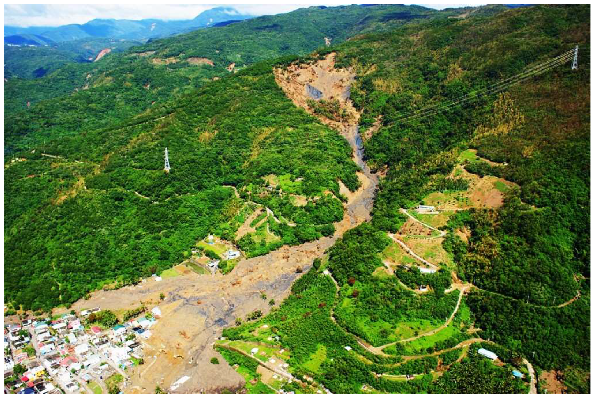
During August 2009, Typhoon Morakot struck Taiwan and caused a considerable sediment disaster in the Daniao stream watershed of Taitung. A shallow landslide and debris flow from rainfall infiltration inducing occurred on the upstream watershed of the Daniao tribe, which was named Taitung DF097. The 2 m × 2 m grid Digital Terrain Model (DTM), before the disaster, applied to the topographic analysis, whose area approximately equaled 52.38 ha; the elevation was distributed from 60 m to 480 m, the slope was distributed from 0° to 52.8°, and the two major directions of the slope pointed to East and East-South. The aerial picture of the disaster is shown in Figure 1. The investigated results of the hazard zone appeared in existing outcrops, and the crushed materials were distributed on both sides. The volume of the hillside collapse exceeded 300,000 m3 and the watershed of almost 14.85 ha was buried [23].
2.2. Geological Properties
The 10 boreholes were drilled to understand the geological characteristics of the collapsed zone, whose soil samples were taken from the split tube samplers, and all of the samples were subjected to a soil properties test in a laboratory. The drilled results had two stratums that exist underground, and whose constructions were inhomogeneous. The geological profile is shown in Figure 2, and the geological characteristics of the collapsed region are shown in Table 1. According to the fundamentals of the Plasticity Chart from Casagrande, the soil type of the collapsed zone could be classified as part of the inorganic clays of low plasticity soil (CL-ML).
2.3. Short Term Water Table Monitoring
The boreholes were also used for the short term monitoring of water tables from 1 July 2010 to 30 September 2010, as shown in Figure 3. In the absence of rainfall, the collapsed zone, borehole BH-3 monitoring results are shown in the water tables around the landslide, which are almost preserved statically at 4.56 m underground. The water table starts to rise when a rainfall in excess 15.5 mm/h occurs. A weekly rainfall occurred from 12 July 2010 to 29 July 2010, and the water tables raised to 2.86 m underground. Next, a maximal rainfall of 63 mm/h occurred at 08:00 on 8 September 2010, and the water tables showed the maximum values of 0.49 m underground.
2.4. Model Inputs
The environmental information all comes from the model inputs, where topographic data are from 2 m × 2 m DTM analysis results; the hyetograph is from Typhoon Morakot rainfall record, and we set the initial infiltration rate Iz = 0 because an infiltration is ignored before a rainfall occurs. The friction angle is selected at a minimal value of inorganic clays in low plasticity soil equal to 18° [24] and the cohesive value is 22 kPa [25]; the hydraulic conductivity of silty clay loam is Ks = 2.382 × 10⁻⁷ m/s [26]; the diffusivity value using D0 = 4.764 × 10⁻⁵ m2/sec is about 200 times of the saturated hydraulic conductivity Ks [27]; the geological parameters are all taken from Table 1. According to the results of that boreholes, the maximal failure depth set 12.65 m underground is equal to the first stratum depth, and the initial water table is from the BH-3 monitoring result, which equals 4.56 m underground.
3. Analysis of Rainfall Infiltration Induced Shallow Landslide
3.1. Rainfall Infiltration
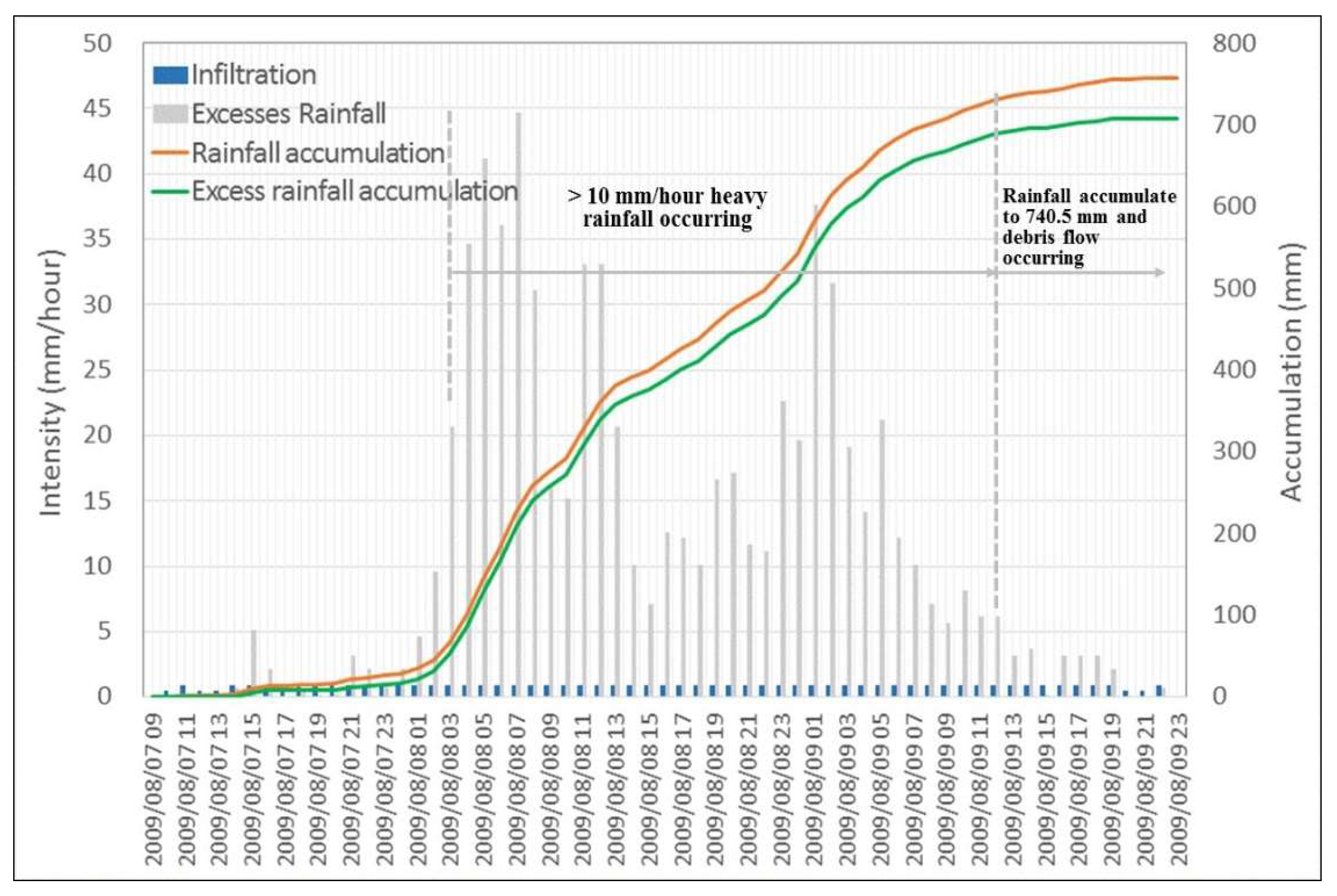
The variable Iz means an infiltration rate; P means the rainfall intensity, RU means the upstream runoff, RD means downstream runoff, and KS means the hydraulic conductivity of soil in saturation. The rainfall infiltration modules of TRIGRS [17,18] have shown that the rainfall would completely infiltrate under a P + RU < KS condition, the infiltration rate Iz = P + RU, and without downstream runoff, RD occurs under this condition. Then, the infiltration rate Iz = KS under P + RU > KS condition, and the downstream runoff RD = P + RU –KS would occur. In this study, rainfall infiltration induced a shallow landslide and debris flow case for the Daniao tribe, and Typhoon Morakot produced heavy rainfall from 09:00 7 August 2009 to 03:00 10 August 2009. The rainstorm accumulated 758 mm in 62 h, and the maximal rainfall intensity reached 45.5 mm/h at 06:00 7 August 2009. The rainstorm accumulation reached 740.5 mm at 15:00 8 August 2009 and induced considerable landslides and debris flow [28]. Because of the Typhoon Morakot’s heavy rainfall, the intensity of the rainfall P was smaller than hydraulic conductivity KS, which only appeared at 1, 3, 5, 8, 59 and 60 h, and the rainfall intensity was all greater than the hydraulic conductivity KS at other times. The hyetography of rainfall infiltration analysis during Typhoon Morakot Struck appears in Figure 4.
3.2. Total Pressure Head Response
The TRIGRS model considers the ground surface boundary with an infiltration rate and a finite depth Zmax as an impermeable boundary, and based on the linear solution of the Richard Equation by Iverson [14], we found a groundwater head φ expressed in Equation (1) [17,18]:
where the first term of the right hand side of Equation (1) means the steady parts, and whose remaining parts represent the transient parts. The equation is used to estimate the water table from a rainfall infiltration, and the equation applies where hydraulic properties are uniform. t is the time variable, Z = z/cos θ is a special variable in vertical coordinate direction (where z is a special variable in slope normal coordinate direction, which means a failure depth on an incline plane), d is an initial depth of the water table measured in Z direction in steady state, dLZ means the depth of an impermeable basal boundary measured in the Z direction, β = λ cos θ, where λ = cos θ – (Iz/Kz)LT, and in which Kz is a hydraulic conductivity in the Z direction and Iz is an initial surface flux, Inz is a surface flux of a given intensity in nth time interval, D1 = D0 cos 2θ (where D0 is the saturated hydraulic diffusivity), a script LT means long term, a script N means total number interval, a form of H(t – tn) is Heavy side function, and a form of the function ierfc means:
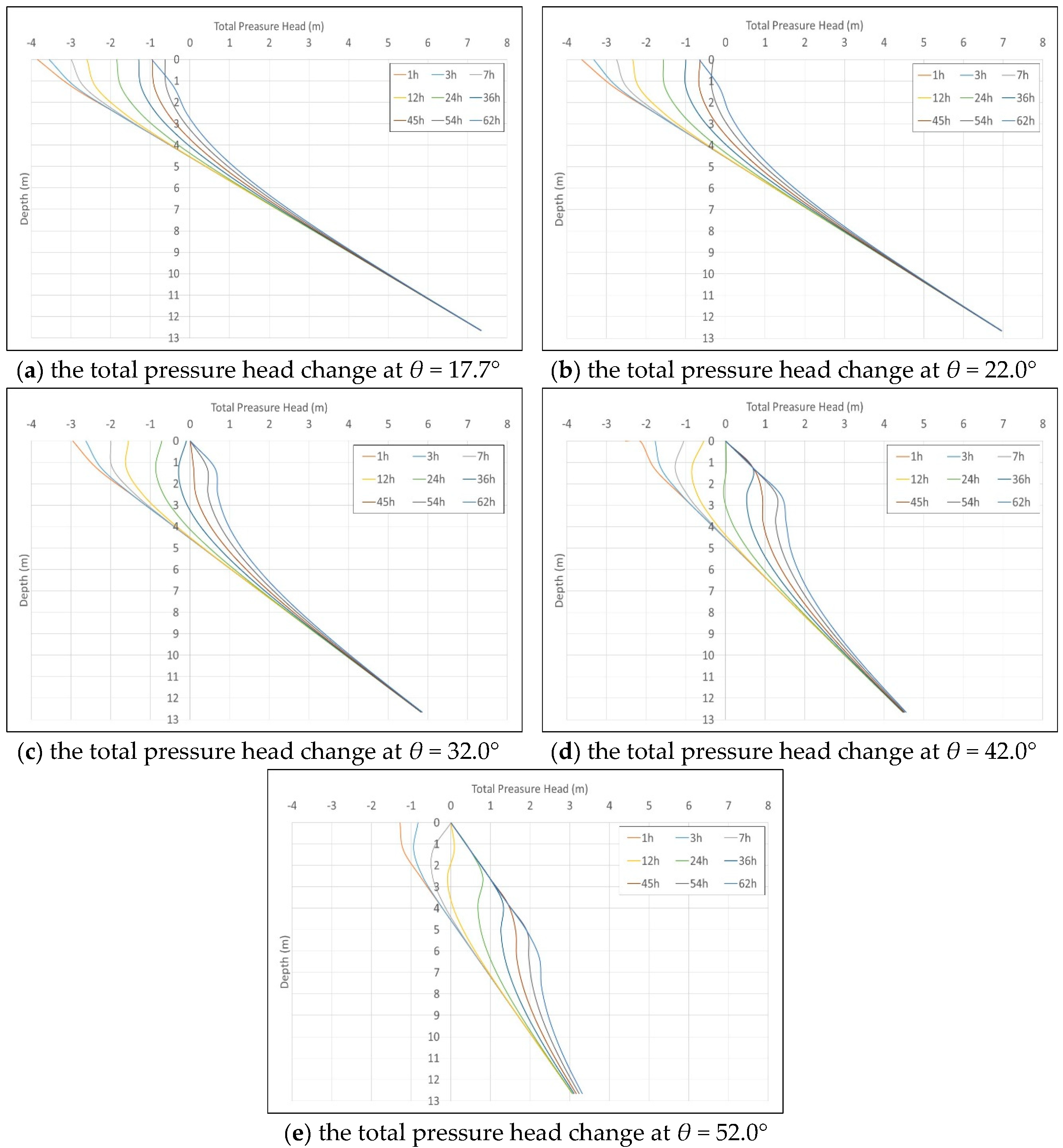
The TRIGRS model is employed as an assessment of the rainfall infiltration that induced a shallow landslide on the Daniao tribe’s hillslope when Typhoon Morakot struck. Figure 5a–e shows the total pressure head change in 1, 3, 7, 12, 24, 36, 45, 54, and 62 h as the slope θ = 17.7°, 22°, 32°, 42°, and 52°, respectively. Because Inz/KZ = 0 before a rainfall occurs, Equation (1) appears as φ = (Z − d) cos2θ, and the total pressure head of groundwater almost maintains a steady state. As a rainfall infiltration has begun to occur, the steady state almost maintains itself until a time equal to 1 h, and the total pressure head is almost similar to a hydrostatic distribution (see the orange color lines in Figure 5a–e). Subsequently, a rainfall infiltration occurs in Inz/KZ > 0, and the β and transient terms of Equation (1) will increase. Therefore, the rainfall infiltration leading to the suction pressure head tends to be smaller in unsaturated regions of soil, and the water table tends to rise (see Figure 5a–e. The phenomena implies that the water content of soil tends to saturate.
Figure 5a shows a total pressure head change significantly increasing as a rainfall infiltration occurs as the slope θ = 17.7°. The total pressure head increased from 0 m to 0.9 m at location Z = 4.56 m (the position of the initial water table), the suction pressure head changed from −3.84 m to −0.62 m at location Z = 0.01 m (near the ground surface), and the groundwater table (the free surface of groundwater) significantly raised from 4.56 m to 2.73 m underground. Figure 5b shows that an analogous total pressure head change occurred at θ = 22°. The total pressure head increased from 0 m to 0.93 m at a location Z = 4.56 m, the suction pressure head changed from −3.62 m to −0.66 m at location Z = 0.01 m, and the groundwater table almost raised from 4.56 m to 2.07 m underground. Comparing both results of Figure 5a,b shows the total pressure head and the water table with higher responses in the more steep zone of the hillside.
Figure 5c–e shows the total pressure head change as rainfall infiltration occur at the slope θ = 32°, 42°, and 52°, respectively. These results have shown that the suction pressure heads gradually reduce and the water tables gradually raise to the ground surface. At a location Z = 0.01, suction pressure heads changed from −2.96 m to 0 m as θ = 32°, from −2.15 m to 0 m as θ = 42° and from −1.28 m to 0 m as θ = 52°. At locations θ = 32°, 42° and 52°, the groundwater tables respectively raised to the ground surface at 45 h, 36 h, and 24 h, and the suction pressure heads dissipated at the same time.
3.3. Safety Factor Response
The TRIGRS model considers a rectangular Cartesian coordinate system with its origin at an arbitrary point on the ground. The x points to the down slope, the y points to tangents the topographic contour, and z normal points to x − y plane, which points into the slope. The model was adopted to an infinite-slope stability analysis model by Iverson [14], where ϕ is a friction angle, θ is a slope angle, C is the cohesion of soil, γw means a unit weight of water, γS is a unit weight of soil, and φ is a groundwater pressure head. FS expresses the failure of the infinite slope, which is characterized by the ratio of resisting basal Coulomb friction to gravitationally induced downslope basal driving stress and called the factor of safety is shown in Equation (3) [17,18]. As the rainfall infiltration (Inz/KZ > 0) would cause the total pressure head of groundwater φ to rise, and the hill would tend to be unstable (FS < 1).
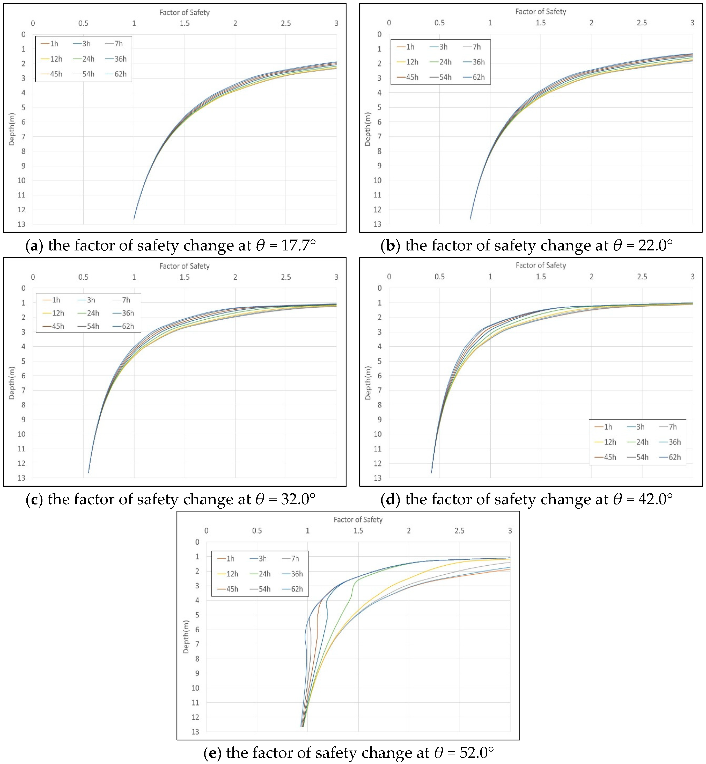
The TRIGRS model is applied to an assessment of the rainfall infiltration that induced a shallow landslide on the Daniao tribe’s hillslope during Typhoon Morakot struck. Figure 6 shows the value of the safety factors that changed in 1, 3, 7, 12, 24, 36, 45, 54, and 62 h, where θ = 17.7°, 22°, 32°, 42°, and 52°. The value of the safety factors would reduce with rainfall infiltration. This phenomena implied the hillside would tend to unstable. Figure 6a shows a factor of safety FS changed at θ = 17.7° due to a rainfall infiltration, where the safety factor were all maintained in FS > 1 during a rainfall infiltration, the result implied that the hillslope were all maintained in a stable state where the slopes satisfied the θ ≤ 17.7° condition. The collapse occurred where the slopes satisfied θ > 17.7° condition, and where the depths were reduced as the slopes increased on the zone that satisfied the θ ≤ 45° condition, but an inverse result occurred as the slope’s θ > 45°. This is because the driving force’s term included a tan θ function (the denominator of Equation (3)). This result implied that the driving force would increase where the slope satisfied θ ≤ 45°, but would reduce where the slope satisfied θ > 45°. Figure 6b–e shows that the factors of safety changed due to a rainfall infiltration at θ = 22°, 32°, 42°, and 52°, and the collapse (FS < 1) occurred at depths that were greater than 8.22 m, 4.09 m, 2.55 m, and 5.68 m, respectively. The results demonstrate such phenomena, too.
3.4. Validation of Potential Collapse Zone
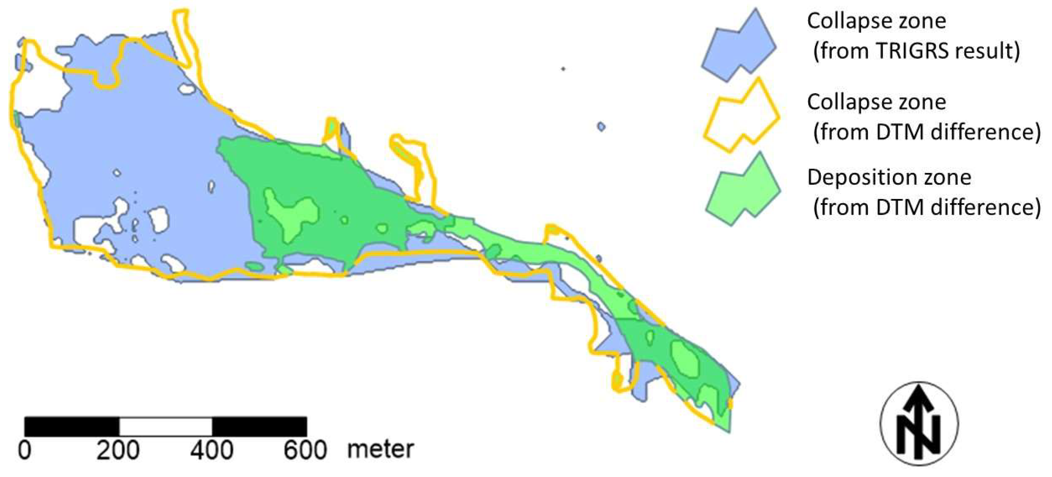
The Taitung branch office of the Soil and Water Conservation Bureau in Taiwan [23] has a record about the difference of the DTM analysis results between before and after the Daniao tribe’s landslide due to Typhoon Morakot, and this information is used to validate the result from the TRIGRS simulation. Figure 7 shows a comparison of the collapse zones, both from the DTM analysis and TRIGRS simulation.
The DTM difference analysis results reveal the terrain with an increase or reduction. The terrain increase range is represented by the green colored block in Figure 7, which is a deposited zone of the landslide. The deposited area equals 26,096 m2, and the deposited volume equals 93,574 m3. The collapsed zone is the region with terrain reduction, whose range is where a yellow color line is included in Figure 7. The collapse area equals 77,969 m2 and the collapsed volume equals 319,875 m3 (without including the deposited zone).
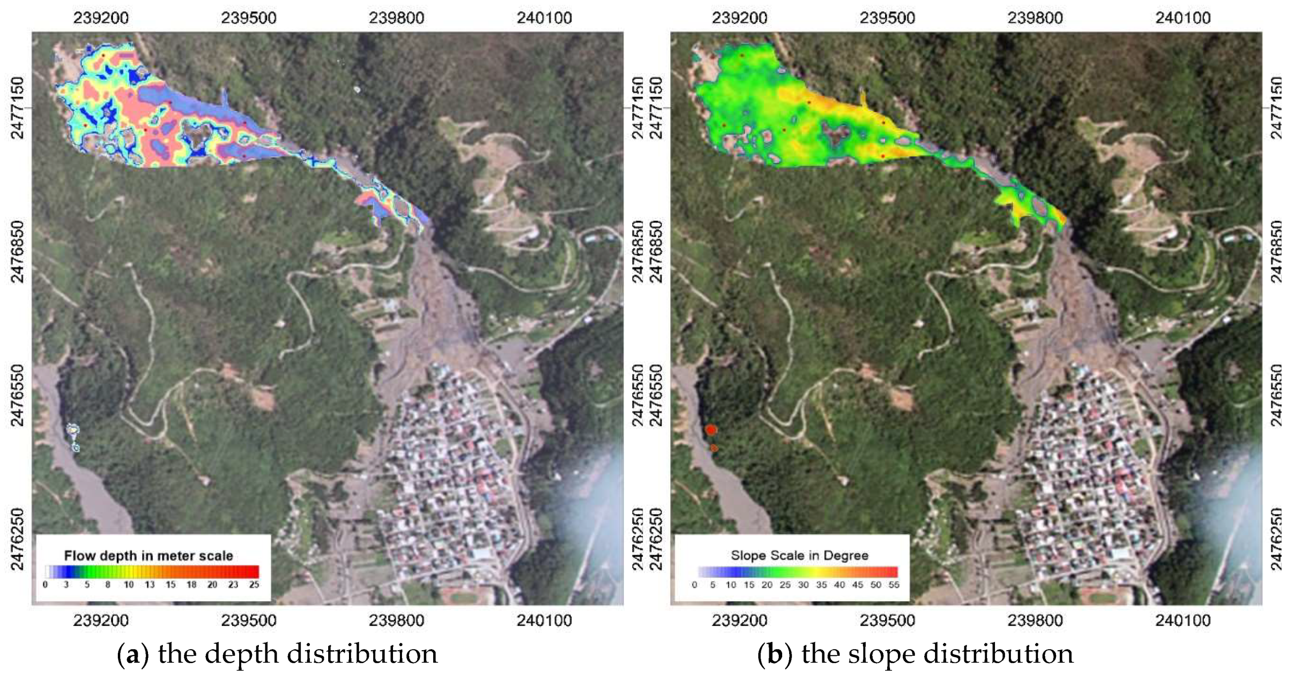
The results of the TRIGRS simulation have revealed the relationships of the total pressure head changes and the factor of safety change with depth. In this study, a threshold condition Fs = 1 is applied to identify the collapsed zone from the simulated TRIGRS results. The collapsed area from TRIGRS’s result with 71,672 m2 is represented by the blue colored block in Figure 7, whose distributions of depth and slope on the collapsed zone are shown in Figure 8a,b, respectively. Therefore, the depth distribution and area of the collapse zone used to calculate the collapsed volume is 391,894 m3 (without including the deposited zone). Therefore, the TRIGRS simulated results are shown with 8% errors for the collapsed area and 23% errors for the collapse volume, compared to the DTM analysis results.
4. Analysis of Subsequent Motion of Collapsed Mass
4.1. Debris Flow Spreading Model and Inputs
The hillside collapsed when factors of safety FS < 1; then, the collapsed mass mixed with enough water and became a debris flow that moved to a downslope. A physical model, DEBRIS-2D, is used to analyze the subsequent motion of the collapsed mass. The DEBRIS-2D model is an adopted depth integral form of the conservation law under long wave approximation in the plug flow region, which was originally developed by Liu and Huang [2]. DEBRIS-2D has an inclined coordinate system, where x coincides with the flow direction, y tangents to a topographical contour direction and z is normal at the x − y plane and points to the depth direction. The velocity components in the x, y directions are u and v respectively, θ is the inclined angle, τ0 is the yield stress, and H = h − B is the flow depth (where h is the free surface and B is the natural bottom of the debris flow). The momentum equations, in conservative form, are shown in Equations (4) and (5), and the continuity equation is shown in Equation (6).
In this study, the DEBRIS-2D model is employed as an assessment of the subsequent motion of the collapsed mass on the upstream of the Daniao tribe. The grid size used was 2 m × 2 m DTM for numerical computation and the time step was established as 0.04 s. The initial velocities when a hillside just fails were u = 0 and v = 0. The TRIGRS result provided the initial volume as 528,063 m3, and the initial depth H distributed on the upstream of Daniao tribe as in Figure 5a. The three unknowns H, u, and v could be solved from three independent Equations (4)–(6).
4.2. Description of Debris Flow Motion
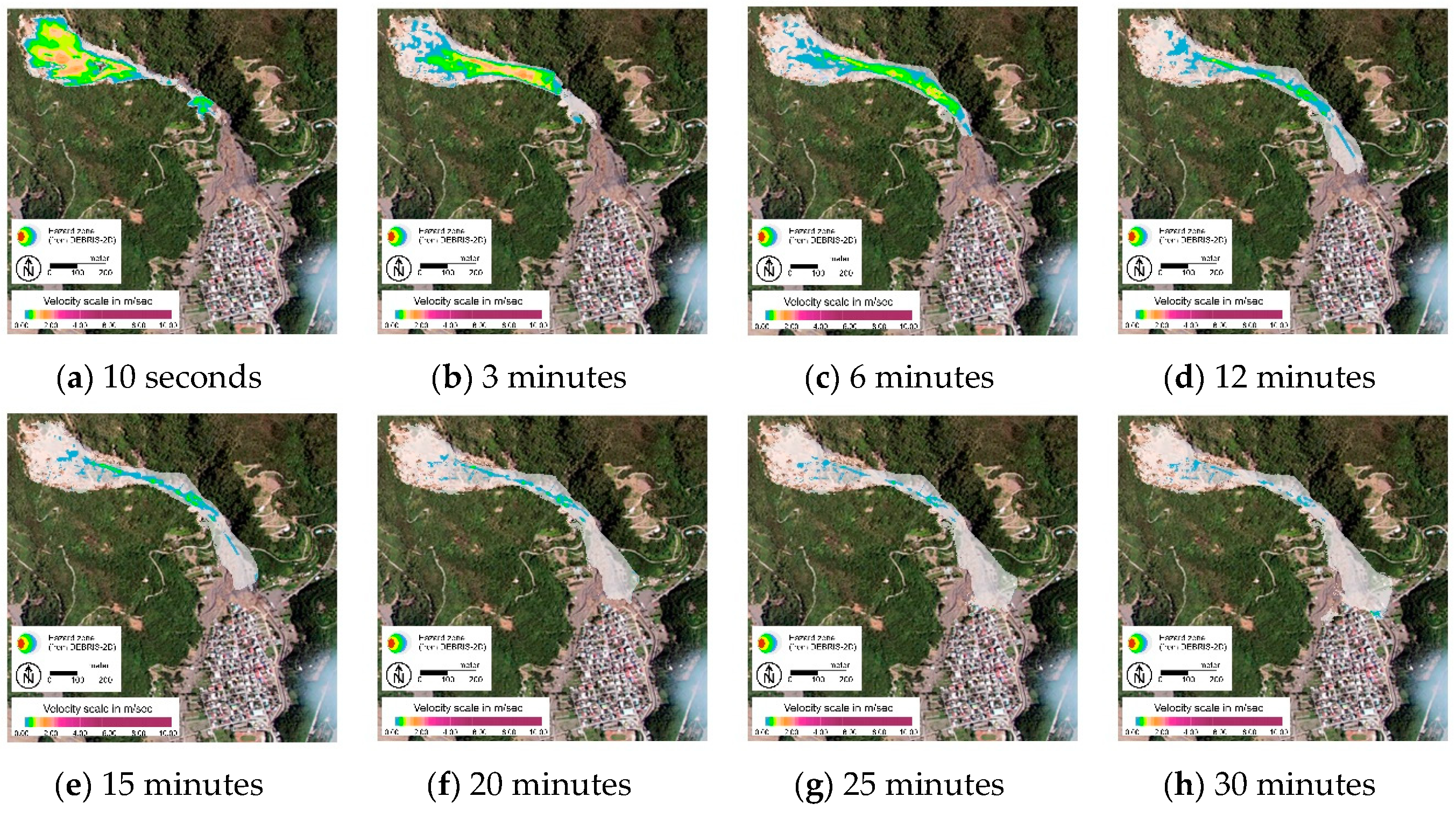
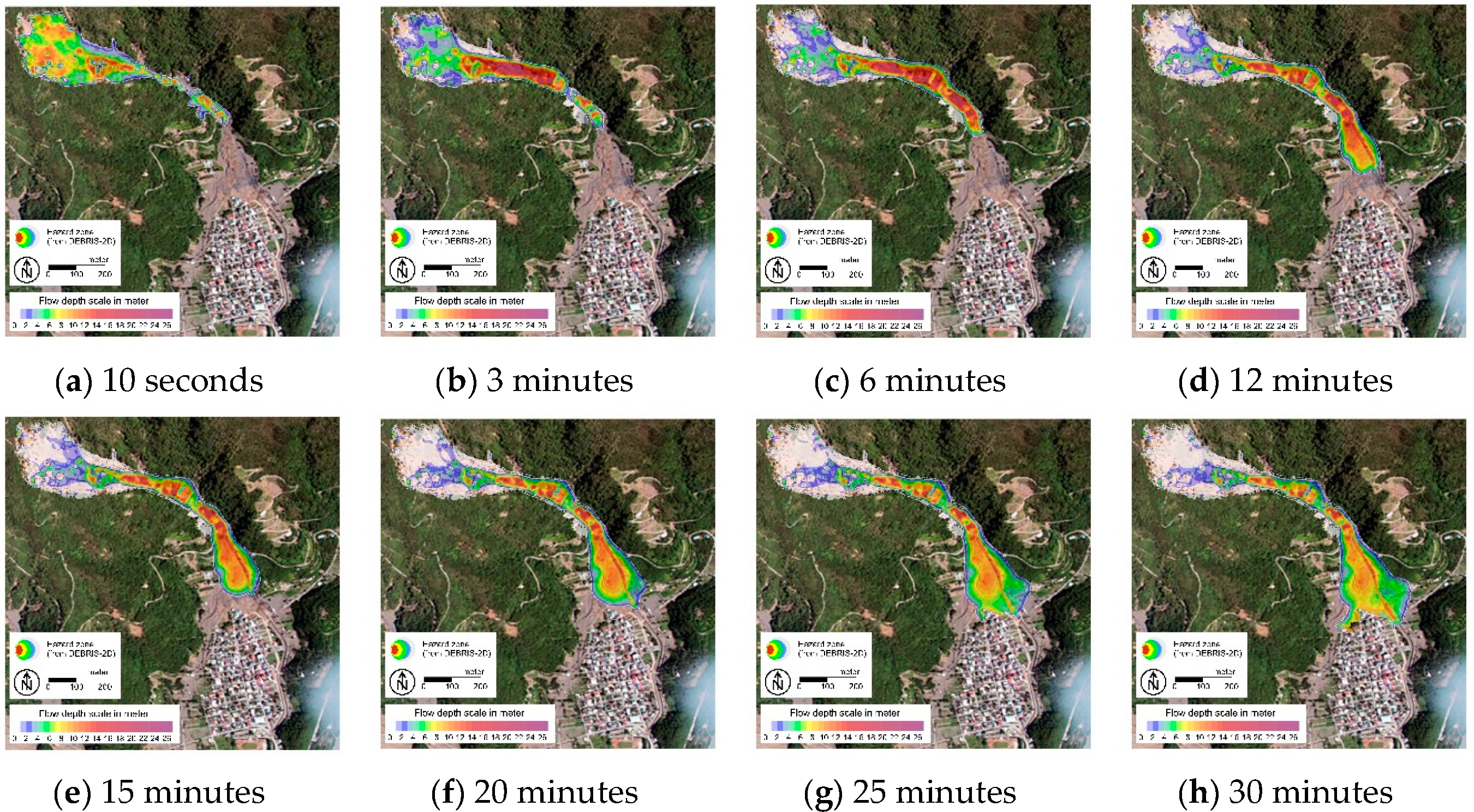
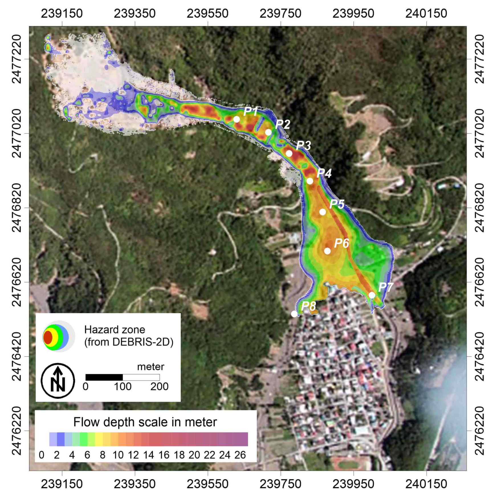
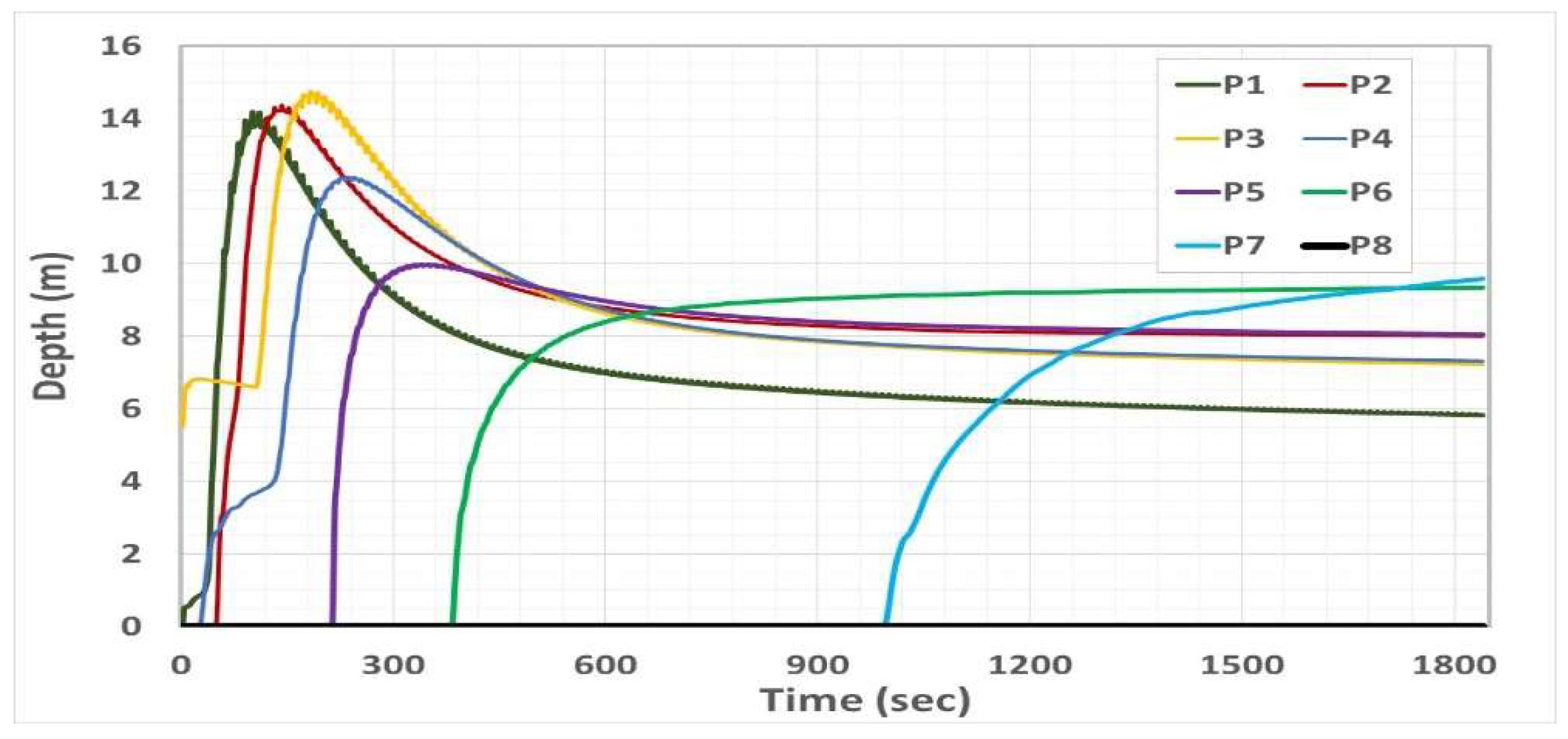
The DEBRIS-2D results show the distributions of velocity and depth as debris flow motion at 10 s and 3, 6, 12, 15, 20, 25, 30 min, which are shown in Figure 9 and Figure 10, respectively. The final deposition of debris flow occurred at 1840 s, as shown in Figure 11. The eight specific points on a valley (see Figure 11, points P1 to P8) are used to record the velocity and depth change as debris flow spreads. The debris flow velocities that changed with time are shown in Figure 12, and the depths that changed with time are shown in Figure 13.
The P1 is located on the upstream of the master check dam (see Figure 11, P1 position). The Debris flow arrives at P1 almost at 28 s and the depth rapidly accumulates. The debris flow depth accumulated to 6.2 m with a velocity that equaled 1.9 m/s at 49 s, and over the check-dam flow to a downstream. The debris flow reached maximal velocity 3.0 m/s as time equaled 67 s and appeared to rapidly reduce afterward (see Figure 12, P1 line), and the depth of debris flow accumulated to a maximum of 14.2 m at 90 s (see Figure 13, P1 line). Figure 9b and Figure 10b show the distributions of velocity and depth as debris flowed over the check dam at 180 s (equal to 3 min). At the P1 position, because of the contraction of the terrain and the countercheck of the dam, the debris flow almost stopped after 1500 s (equal to 25 min) (see Figure 9g,h) and the depth almost remained at 6 m (see Figure 10g,h)
The P2 is located between the master check-dam and minor-check dam (see Figure 11, P2 position). The debris flow arrived at P2 at a time equal to 53 s, and the debris flow crossed the minor check-dam with a flow velocity of 0.40 m/s and a flow depth of 8.2 m at 86 s, then flowed to the downstream. The debris flow reached a maximal depth of 14.3 m, which occurred at 132 s (see Figure 13, P2 line), and a maximal velocity of 1.43 m/s occurred at 139 s (see Figure 12, P2 line). The velocity of the debris flow was almost smaller than 0.01 m/s (see Figure 12, P2 line), and the depth remained at 8.3 m (see Figure 13, P2 line), which occurred at 672 s and the motion almost stopped. Figure 9b–d and Figure 10b–d show the distributions of velocities and depths of the process.
The P3 is located at a gap in the midstream valley (see Figure 11, P3 position). The bend collapsed mass accumulated with 5.6 m in the P3 position, whose mass start motion has a velocity of 0.71 m/s and flowed to the downstream, with a flow velocity smaller than 0.01 m/s after 34 s (see Figure 12, P3 line), and the depth almost remained at 6.6 m until the time equaled 113 s (see Figure 13, P3 line). Afterward, the upstream debris flow arrived at the P3 position (see Figure 9c and Figure 10c, and the flow velocity rapidly rose to a maximal velocity of 1.58 m/s at 160 s (see Figure 12, P3 line), and the flow depth rapidly increased to a maximal depth 14.7 m at 191 s (see Figure 13, P3 line). The flow velocity reduced, then, to 0.01 m/s at a time equal to 850 s, the debris flow tended to stop (see Figure 12, P3 line), and the depth reduced from 8.5 m to 7.3 m (see Figure 13, P3 line and Figure 10e–h).
The P4 is located on the upstream of the valley mouth (see Figure 11, P4 position). Two components of the debris flow have crossed the P4 position. The first component reaches the P4 position at 35 s and with a velocity of 0.1 m/s and a depth of 1.4 m. The secondary component reaches the P4 position at 129 s with a velocity 0.2 m/s and a depth 3.9 m (see Figure 12 and Figure 13, P4 line). The flow velocity rapidly rose to a maximal value of 1.89 m/s at 187 s, and respectively reduces to 1 m/s, 0.5 m/s, and 0.3 m/s as the time equaled to 375 s, 631 s, and 1064 s (see Figure 9d–f). Afterward, the velocity reduced very slowly until the time equaled to 1840 s, and the flow velocity reduced from 0.3 to 0.21 m/s (see Figure 9g,h). The depth of the debris flow rapidly increased to a maximal value of 12.4 m at 234 s and reduced smaller than 9 m at 554 s (see Figure 10c,d). Afterward, the depth became sluggish until the time equaled to 1840 s, and the flow depth reduced from 9 to 7.31 m (see Figure 10 e–h).
Locations P5 and P6 are located on the valley mouth (see Figure 11, P5 and P6 positions). The debris flow crossed the P5 and P6 positions at 216 and 389 s, respectively. The flow velocity reached a maximal value of 0.96 m/s at P5 at a time equal to 226 s (see Figure 12, P5 line), and 0.42 m/s at P6 at a time equal to 399 s (see Figure 12, P6 line). At the P5 position, the flow depth rapidly accumulated to a maximal depth of 9.97 m from 216 to 330 s, and then appeared to mildly reduce. The final depth was almost maintained at 8 m (see Figure 13, P5 line). At the P6 position, the flow depth rapidly accumulated to 8.40 m from 389 to 602 s; then, the flow depth was maintained and gently accumulated to a maximal value of 9.34 m at 1840 s (see Figure 13, P6 line). Because the terrain became broad, the debris flow fan started to become revealed (see Figure 10d–h), and the flow velocity abated significantly (see Figure 9d–h). On the P5 and P6 positions, the flow velocities reduced smaller than 0.1 m/s, respectively, at 973 and 753 s, and the motion almost stopped.
The debris flow arrived at the Daniao tribe almost at 20 min (see Figure 9f), because the buildings obstructed the debris flow attacks, the plug occurred at the upstream of the Daniao tribe, and the depth accumulates almost at 8 to 10 m (see Figure 10f–h; Figure 11). Then, the debris flow overflowed to both sides. The P7 and P8 are located on both sides of the Daniao tribe (see Figure 11, P7 and P8 positions). Two components of the debris flow crossed P7. The first component came from the upstream ditch, and the debris flow component arrived at P7 at 994 s (see Figure 10f and Figure 12, P7 line). The second component is the overflow from the upstream of the Daniao tribe, which almost occurred at 20 to 25 min (see Figure 9f,g). The maximal velocity of debris flow of 0.23 m/s appeared at 1073 s (see Figure 12, P7 line); the flow depth maintained accumulation ot the P7 position and the maximal depth of 9.57 m occurred at 1840 s (see Figure 13, P7 line). Afterward, the velocity of the debris flow reduced to 0.03 m/s and almost stopped (see Figure 12, P7 line). On the other side, the debris flow stopped before arriving at the P8 position, and the upstream accumulation depth was almost 2 to 6 m (see Figure 11).
4.3. Validation of Hazard Zone
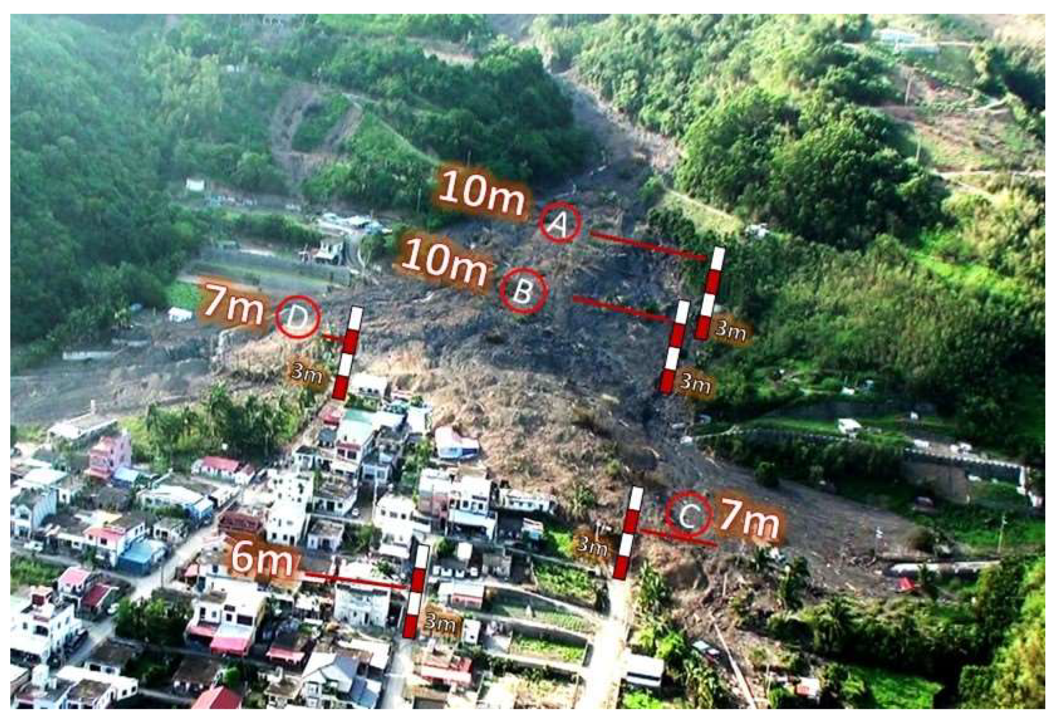
The aerial photo after the Daniao tribe’s disaster and the investigated results would be used to validate the simulated results from DEBRIS-2D. The interlaced line composed of red and yellow colors was used to depict the disaster range from the aerial map and overlapped the DEBRIS-2D simulated result (colored contours) for comparison, as shown in Figure 14. The depicted result shows that the range of the debris flow of the disaster was 117,480 m2; the DEBRIS-2D result appeared in the hazard zone with 146,316 m2 and with a 25% positive error relative to the real hazard zone. In spite of that, the hazard zone from the DEBRIS-2D simulation could almost include the real disaster range. Figure 15 shows a photo of the Daniao tribe’s debris flow fan, and we used the features of the landscape in the photo as the scale for estimating the deposited depth of the debris flow. Roughly estimated, the deposited depths were 10 m, 10 m, 7 m, and 7 m on the A, B, C, and D location, respectively (see Figure 15). However, the DEBRIS-2D results are shown at 10 m, 10 m, 8 m and 6 m on the locations (see Figure 14).
5. Conclusions
This study combines the TRIGRS and DEBRIS-2D models to simulate rainfall infiltration inducing a shallow landslide and the subsequent motion of debris flow. The combining model is applied to a real disaster case analysis of the Daniao tribe hill, and all parameters input into the model were obtained from field measurements and monitoring.
TRIGRS revealed that the total pressure head and safety factor changed according to rainfall infiltration, and show that the free surface of groundwater gradually raises to the ground surface during a rainfall infiltration. The phenomena implies that the water content of soil is gradually saturated. At the same time, the suction pressure head in the unsaturated region dissipates, and the groundwater pressure head increases. The changes of the safety factor processes show that the safety factor reduces. The hillside collapse occurred when the safety factor reduced to Fs = 1, and the collapse zone and collapse depth were identified by the locations that would satisfy the condition Fs = 1. Therefore, TRIGRS revealed the collapsed zone as well as failure depth distribution.
Afterward, DEBRIS-2D adopted the TRIGRS’s results for simulation of the subsequent motion of debris flow and hazard zone assessment. In this study, we set up eight specific points on a valley to measure velocity and depth of debris flow. The simulation showed that the debris flow appeared at a higher speed on the steep region of a valley during the beginning of motion; as the debris flow crossed the check dam or gaps in the upstream valley, the flow velocities reduced very significantly, and depth accumulation occurred. Afterward, the debris flow ran out of the valley mouth, and the debris flow spread to both sides. The flow velocities almost dissipated, and the debris flow fan formed. The hazard zone simulation from DEBRIS-2D matches the actual disaster region well. However, DEBRIS-2D could not reveal an actual situation where the check dam was destroyed by debris flow.
The area and volume of the collapse zone from the TRIGRS simulation within 8% and 23% errors from a comparison of the DTM variation analysis of before and after a landslide. Further, the debris flow hazard zone of DEBRIS-2D simulation was within 25% errors from the comparison of a disaster aerial photo. The combining model applied to the simulation of a rainfall infiltration induced landslide and, subsequently, the model was applied to the debris flow of Daniao tribe disaster case, a real disaster range with a nearly 75% match. In spite of this match, the hazard zone from the simulation still included a real disaster range, the simulated results that were well-matched with the real case of the Daniao tribe.
Therefore, we believe that the combining method of the study would provide a better solution for disaster assessment. Two contributions of our work are: (1) to identify the collapsed zone and map the mapping of the hazard zone’s subsequent motion. (2) These results have potential application in large range sediment disaster prediction and would be of great help in the management of slope disaster prevention.
Author Contributions
Y.-C.H. performed the works of: Conceptualization, Data curation, Formal analysis, Investigation, Methodology, Project administration, Resources, Software, Validation, Writing—original draft, and Writing—review & editing; K.-F.L. assisted the work of: Supervision.
Funding
This research was supported by Soil and Water Conservation Bureau (SWCB) in Taiwan through Grant No.108AS-10.10.1-SB-S3, and partial support by Ministry of Science and Technology (MOST) in Taiwan through Grant No. 107-2625-M-002-015.
Acknowledgments
The authors wish to thank the Taitung Branch office of the Soil and Water Conservation Bureau in Taiwan for providing information. We would also like to thank the anonymous reviewers for their valuable remarks and comments that greatly improved the quality of the paper.
Conflicts of Interest
The authors declare no conflict of interest.
References
- O’Brien, J.S.; Julien, P.Y.; Fullerton, W.T. Two-dimensional water flood and mudflow simulation. J. Hydraul. Eng. 1993, 119, 224–261. [Google Scholar] [CrossRef]
- Liu, K.F.; Huang, M.C. Numerical simulation of debris flow with application on hazard area mapping. Comput. Geosci. 2006, 10, 221–240. [Google Scholar] [CrossRef]
- Tsai, M.P.; Hsu, Y.C.; Li, H.C.; Shu, H.M.; Liu, K.F. Application of simulation technique on debris hazard zone delineation: A case study in the Daniao tribe, Eastern Taiwan. Nat. Hazards Earth Syst. Sci. 2011, 11, 3053–3062. [Google Scholar] [CrossRef]
- Piccarreta, M.; Pasini, A.; Capolongo, D.; Lazzari, M. Changes in daily precipitation extremes in the Mediterranean from 1951 to 2010: The Basilicata region, Southern Italy. Int. J. Climatol. 2013, 33, 3229–3248. [Google Scholar] [CrossRef]
- Lazzari, M.; Piccarreta, M.; Capolongo, D. Landslide triggering and local rainfall thresholds in Bradanic Foredeep, Basilicata region (Southern Italy). Landslide Sci. Pract. 2013, 2, 671–676. [Google Scholar] [CrossRef]
- Lazzari, M.; Piccarreta, M. Landslide disasters triggered by extreme rainfall events: The case of Montescaglioso (Basilicata, Southern Italy). Geosciences 2018, 2, 377. [Google Scholar] [CrossRef]
- Lazzari, M.; Piccarreta, M.; Manfreda, S. The role of antecedent soil moisture conditions on rainfall-triggered shallow landslides. Nat. Hazards Earth Syst. Sci. 2018. [Google Scholar] [CrossRef]
- Collins, B.D.; Znidarcic, D. Stability analyses of rainfall induced landslides. J. Geotech. Geoenviron. Eng. 2004, 130, 362–372. [Google Scholar] [CrossRef]
- Conte, E.; Troncone, A. A method for the analysis of soil slips triggered by rainfall. Geotechnique 2012, 62, 187–192. [Google Scholar] [CrossRef]
- Conte, E.; Donato, A.; Troncone, A. A simplified method for predicting rainfall-induced mobility of active landslides. Landslides 2017, 14, 35–45. [Google Scholar] [CrossRef]
- Alonso, E.E.; Gens, A.; Delahaye, C.H. Influence of rainfall on the deformation and stability of a slope in overconsolidated clays: A case of study. Hydrogeol. J. 2003, 11, 174–192. [Google Scholar] [CrossRef]
- Conte, E.; Troncone, A. Stability analysis of infinite clayey slopes subjected to pore pressure changes. Geotechnique 2012, 62, 87–91. [Google Scholar] [CrossRef]
- Conte, E.; Troncone, A. A performance-based method for the design of drainage trenches used to stabilize slopes. Eng. Geol. 2018, 239, 158–166. [Google Scholar] [CrossRef]
- Iverson, R.M. Landslide triggering by rain infiltration. Water Resour. Res. 2000, 36, 1897–1910. [Google Scholar] [CrossRef] [Green Version]
- Ali, A.; Huang, J.; Lyamin, A.V.; Sloan, S.W.; Griffiths, D.V.; Cassidy, M.J.; Li, J. Simplified quantitative risk assessment of rainfall-induced landslides modelled by infinite slopes. Eng. Geol. 2014, 179, 102–116. [Google Scholar] [CrossRef]
- Conte, E.; Donato, A.; Pugliese, L.; Troncone, A. Analysis of the Maierato landslide (Calabria, Southern Italy). Landslides 2018, 15, 1935–1950. [Google Scholar] [CrossRef]
- Baum, R.L.; Savage, W.Z.; Godt, J.W. TRIGRS—A Fortran Program for Transient Rainfall Infiltration and Grid-Based Regional Slope-Stability Analysis; US Geological Survey Open-File Report; US Geological Survey: Reston, VA, USA, 2002.
- Baum, R.L.; Godt, J.W.; Savage, W.Z. Estimation the timing and location of shallow rainfall-induced landslides using a model for transient, unsaturated infiltration. J. Geophys. Res. 2010, 115, F03013. [Google Scholar] [CrossRef]
- Chiang, S.H.; Chang, K.T.; Mondini, A.C.; Tsai, B.W.; Chen, C.Y. Simulation of event-based landslides and debris flows at watershed level. Geomorphology 2012, 138, 306–618. [Google Scholar] [CrossRef]
- Hsu, S.M.; Wen, H.Y.; Chen, N.C.; Hsu, S.Y.; Chi, S.Y. Using an integrated method to estimate watershed sediment yield during heavy rain period: A case study in Hualien County, Taiwan. Nat. Hazards Earth Syst. Sci. 2012, 12, 1949–1960. [Google Scholar] [CrossRef]
- Gomes, R.A.T.; Guimaraes, R.F.; Carvalho Júnior, O.A.; Fernandes, N.F.; Amaral, E.V., Jr. Combining spatial models for shallow landslides and debris flows prediction. Remote Sens. 2013, 5, 2219–2237. [Google Scholar] [CrossRef]
- Wang, C.; Marui, H.; Furuya, G.; Watanabe, N. Two integrated models simulating dynamic process of landslide using GIS. Landslide Sci. Pract. 2013, 3, 389–395. [Google Scholar] [CrossRef]
- The Planning of Conservation and Investigation in the Watershed of Daniao Stream; Taitung Branch Office of Soil and Water Conservation Bureau in Taiwan: Taitung County, Taiwan, 2011. (In Chinese)
- Geotechdata.info: Angle of Friction. Available online: http://geotechdata.info/parameter/angele-of- friction.html (accessed on 14 September 2013).
- Geotechdata.info: Cohesion. Available online: http://geotechdata.info/parameter/cohesion (accessed on 15 December 2013).
- Rawls, W.J.; Brakensiek, D.L. A procedure to predict Green Ampt infiltration parameters. In Advances in Infiltration; ASAE Publication: St Joseph, MI, USA, 1983; pp. 102–112. [Google Scholar]
- Liu, C.N.; Wu, C.C. Mapping susceptibility of rainfall triggered shallow landslides using a probabilistic approach. Environ. Geol. 2008, 55, 907–915. [Google Scholar] [CrossRef]
- Investigate Report of Debris Flow Disaster on Daniao Tribe; Taitung Branch office of Soil and Water Conservation Bureau in Taiwan: Taitung County, Taiwan, 2009. (In Chinese)
Figure 1.
Aerial photo of a sediment disaster on the Daniao tribe in eastern Taiwan.

Figure 2.
The geological profile of the collapsed region on the upstream of Daniao tribe.

Figure 3.
A short term monitoring of water tables from 1 July 2010 to 30 September 2010.

Figure 4.
Hyetography of rainfall infiltration.

Figure 5.
The total pressure heads change due to a rainfall infiltration at 1, 3, 7, 12, 24, 36, 45, 54, and 62 h where slopes equal to 17.7°, 22°, 32°, 42°, and 52°.
Figure 5.
The total pressure heads change due to a rainfall infiltration at 1, 3, 7, 12, 24, 36, 45, 54, and 62 h where slopes equal to 17.7°, 22°, 32°, 42°, and 52°.

Figure 6.
The factors of safety change due to rainfall infiltration at 1, 3, 7, 12, 24, 36, 45, 54, and 62 h where slopes equal to 17.7°, 22°, 32°, 42°, and 52°.
Figure 6.
The factors of safety change due to rainfall infiltration at 1, 3, 7, 12, 24, 36, 45, 54, and 62 h where slopes equal to 17.7°, 22°, 32°, 42°, and 52°.

Figure 7.
The comparison of collapse zone.

Figure 8.
The distributions of depth and slope on a potential collapse zone.

Figure 9.
The velocity distributions results of debris flow spreading from the DEBRIS-2D simulation.
Figure 9.
The velocity distributions results of debris flow spreading from the DEBRIS-2D simulation.

Figure 10.
The depth distributions results of debris flow spreading from the DEBRIS-2D simulation.

Figure 11.
The final deposition of the debris flow.

Figure 12.
The velocities changed with time on the specific points.

Figure 13.
The depths changed with time on the specific points.

Figure 14.
The comparison of the hazard zone.

Figure 15.
The photo of the Daniao tribe’s debris flow fan.


Table 1.
Geological Characteristics of the Daniao Tribe’s Landslide.
| Soil Layer | Distributed Depth (m) | Material Constituted | SPT Number (N) | Unit Weight (ton/m3) | Water Content (%) | Porosity Ratio | Liquid Limit LL (%) | Plasticity Index PI (%) |
|---|---|---|---|---|---|---|---|---|
| Brown clastic rock, concrete, gray sand backfill layer | From 0.00 m to 12.65 m underground | Collapse, Backfill layer | 8–>100 | 2.11–2.28 | 6.7–12.7 | 0.26–0.43 | 17.2–19.2 | 6.8–8.7 |
| Average 62.2 | Average 2.21 | Average 8.9 | Average 0.32 | Average 18.5 | Average 8 | |||
| Brown, gray, black and gray broken slate, shear gouge, and rust-strained quartz | From 0.75 m to 50 m underground | Broken Slate | 50–>100 | 1.86–2.20 | 8.5–9.8 | 0.31–0.57 | 17.6–19.5 | 6.8–9.5 |
| Average 69.0 | Average 2.03 | Average 9.0 | Average 0.45 | Average 18.4 | Average 8 |
© 2019 by the authors. Licensee MDPI, Basel, Switzerland. This article is an open access article distributed under the terms and conditions of the Creative Commons Attribution (CC BY) license (http://creativecommons.org/licenses/by/4.0/).
Share and Cite
MDPI and ACS Style
Hsu, Y.-C.; Liu, K.-F. Combining TRIGRS and DEBRIS-2D Models for the Simulation of a Rainfall Infiltration Induced Shallow Landslide and Subsequent Debris Flow. Water 2019, 11, 890. https://doi.org/10.3390/w11050890
AMA Style
Hsu Y-C, Liu K-F. Combining TRIGRS and DEBRIS-2D Models for the Simulation of a Rainfall Infiltration Induced Shallow Landslide and Subsequent Debris Flow. Water. 2019; 11(5):890. https://doi.org/10.3390/w11050890
Chicago/Turabian StyleHsu, Yu-Charn, and Ko-Fei Liu. 2019. "Combining TRIGRS and DEBRIS-2D Models for the Simulation of a Rainfall Infiltration Induced Shallow Landslide and Subsequent Debris Flow" Water 11, no. 5: 890. https://doi.org/10.3390/w11050890
Note that from the first issue of 2016, this journal uses article numbers instead of page numbers. See further details here.