Spatial Characteristics and Temporal Evolution of Chemical and Biological Freshwater Status as Baseline Assessment on the Tropical Island San Cristóbal (Galapagos, Ecuador)

 , ,
, ,  ,
,
Abstract
:1. Introduction
2. Materials and Methods
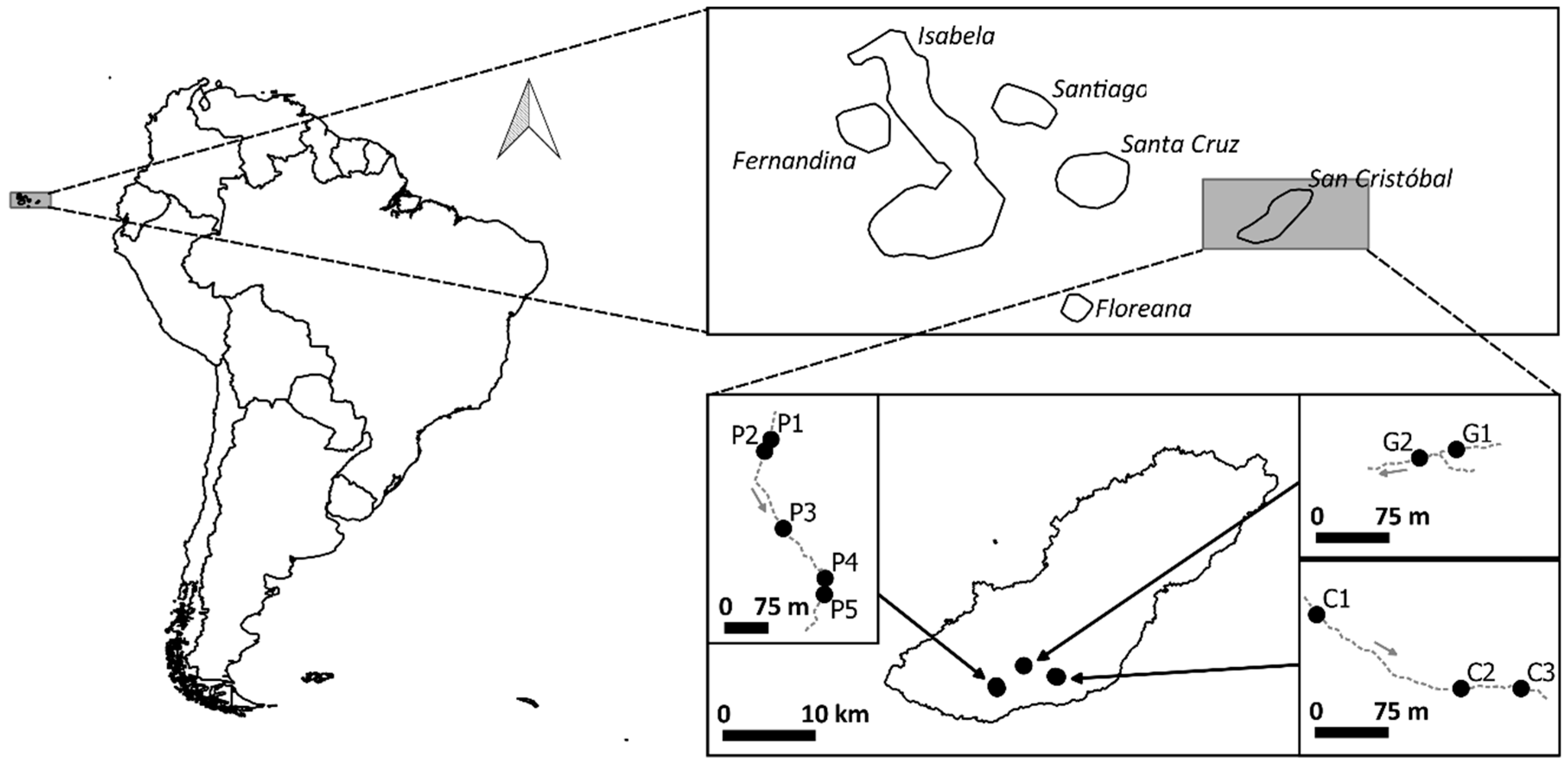
2.1. Site Description and Data Collection
2.2. Data Exploration and Analysis
3. Results
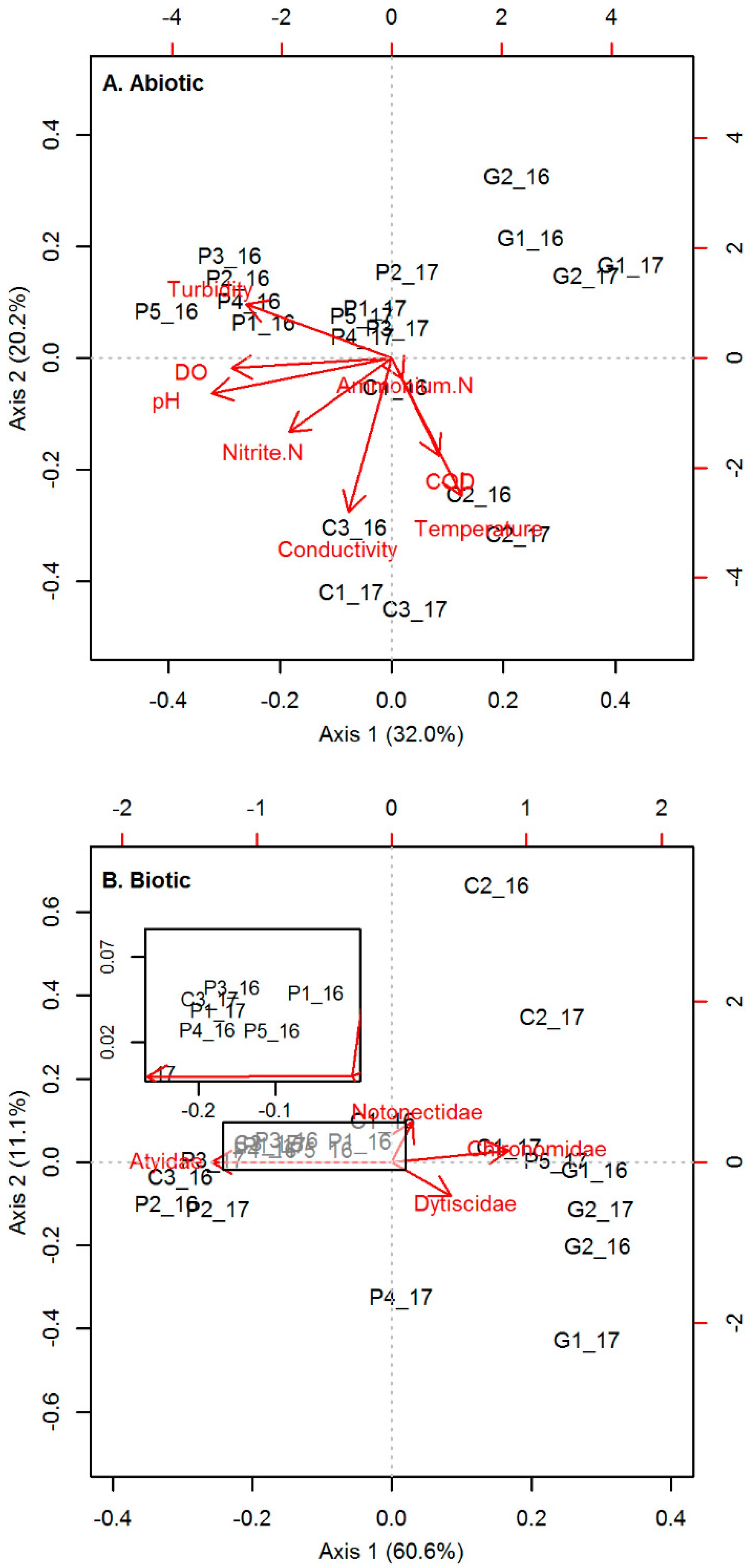
3.1. Baseline Data and Spatial Analysis
3.1.1. Abiotic Conditions
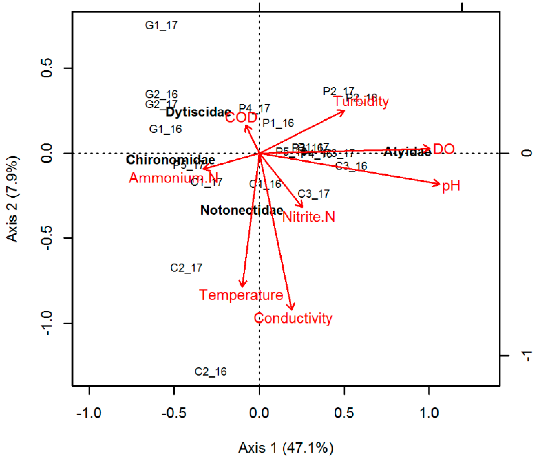
3.1.2. Biotic Conditions
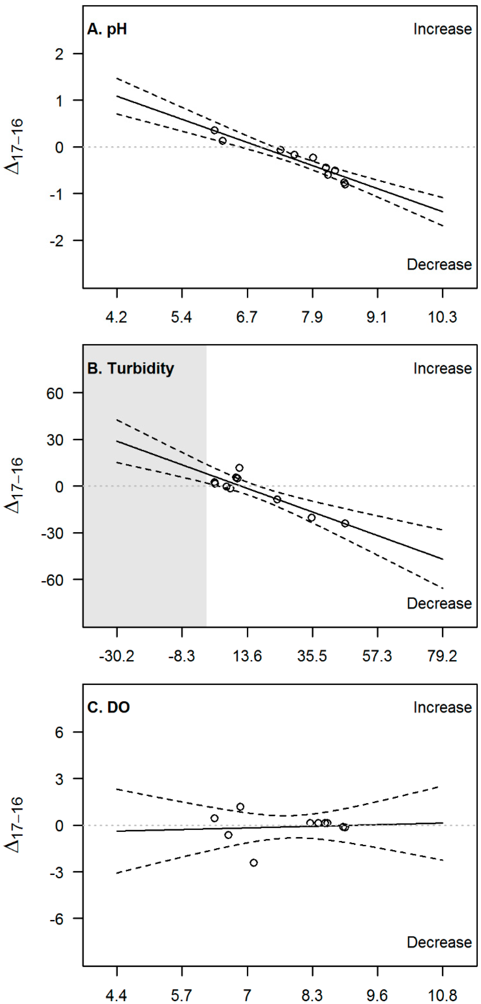
3.2. Temporal Evolution
4. Discussion
4.1. Baseline Data and Spatial Analysis
4.2. Temporal Evolution and Implications
5. Conclusions
Author Contributions
Funding
Acknowledgments
Conflicts of Interest
Appendix A

| Variable | Technique | Remark(s) |
|---|---|---|
| Temperature | Probe | 2016: YSI V6920; 2017: Aquaread AP5000 |
| Conductivity | Probe | 2016: YSI V6920; 2017: Aquaread AP5000 |
| pH | Probe | 2016: YSI V6920; 2017: Aquaread AP5000 |
| Dissolved oxygen | Probe | 2016: YSI V6920; 2017: Aquaread AP5000 |
| Turbidity | 2016: Turbidimeter 2017: Probe | 2016: Hach 2017: Aquaread AP5000 |
| Chemical oxygen demand | Test kit code 2415815 | Hach, limits: 0.7–40.0 mgO2 L−1; follows EPA 5220 D |
| Ammonia-nitrogen | Test kit code 114752 | Merck, limits: 0.010–3.00 mg N L−1; follows EPA 350.1, APHA 4500-NH3 F, ISO 7150-1, and DIN 38406-5 |
| Nitrite-nitrogen | Test kit code 114776 | Merck, limits: 0.002–1.00 mg N L−1; follows EPA 354.1, APHA 4500-NO2-B, and DIN EN 26 777 |
| Nitrate-nitrogen | Test kit code 109713 | Merck, limits: 0.1–25.0 mg N L−1; follows DIN 38405-9 |
| Orthophosphate-phosphorus | Test kit code 114848 | Merck, limits: 0.0025–5.00 mg P L−1; follows EPA 365.2 + 3, APHA 4500-P E, and DIN EN ISO 6878 |
Appendix B
| Taxon | TS | 2016 | 2017 | ||||||||||||||||||
|---|---|---|---|---|---|---|---|---|---|---|---|---|---|---|---|---|---|---|---|---|---|
| P1 | P2 | P3 | P4 | P5 | C1 | C2 | C3 | G1 | G2 | P1 | P2 | P3 | P4 | P5 | C1 | C2 | C3 | G1 | G2 | ||
| Atyidae | 8 | 253 | 349 | 366 | 191 | 313 | 88 | 1 | 636 | 221 | 341 | 595 | 8 | 2 | 13 | 3 | 96 | ||||
| Lymnaeidae | 8 | 2 | 1 | ||||||||||||||||||
| Palaemonidae | 8 | 1 | |||||||||||||||||||
| Planorbidae | 8 | 1 | 1 | 8 | 2 | 3 | |||||||||||||||
| Coenagrionidae | 7 | 2 | 2 | 15 | 6 | 3 | 23 | ||||||||||||||
| Hyalellidae | 7 | 98 | 46 | 7 | 60 | ||||||||||||||||
| Simuliidae | 7 | 1 | 4 | 2 | 1 | 4 | 50 | 2 | |||||||||||||
| Veliidae | 7 | 11 | 44 | 6 | 10 | 25 | 3 | ||||||||||||||
| Aeshnidae | 6 | 5 | 3 | 2 | 10 | 1 | 2 | 1 | 1 | 15 | 9 | 12 | 2 | 1 | |||||||
| Dugesiidae | 6 | 1 | |||||||||||||||||||
| Pleidae | 6 | 2 | |||||||||||||||||||
| Staphylinidae | 6 | 1 | |||||||||||||||||||
| Ceratopogonidae | 5 | 1 | |||||||||||||||||||
| Gyrinidae | 5 | 12 | 14 | 31 | 9 | 1 | 3 | 3 | 3 | 2 | |||||||||||
| Mesoveliidae | 5 | 3 | |||||||||||||||||||
| Notonectidae | 5 | 15 | 25 | 1 | |||||||||||||||||
| Hydrophilidae | 3 | 1 | 1 | 5 | 3 | 1 | 6 | 6 | 5 | 2 | 2 | ||||||||||
| Chironomidae | 2 | 346 | 1 | 159 | 56 | 198 | 145 | 13 | 9 | 683 | 120 | 84 | 27 | 57 | 7 | 327 | 175 | 115 | 22 | 168 | 37 |
| Tubificidae | 1 | 1 | 1 | 1 | 2 | 6 | 7 | ||||||||||||||
| Dytiscidae | - | 1 | 1 | 1 | 29 | 26 | 7 | 3 | 3 | 1 | 5 | 230 | 7 | ||||||||
| Lumbricidae | - | 5 | 6 | 10 | 10 | ||||||||||||||||
| Lumbriculidae | - | 9 | 8 | 4 | 7 | 11 | 9 | 9 | 12 | 7 | |||||||||||
References
- Hughes, S.J.; Malmqvist, B. Atlantic Island freshwater ecosystems: challenges and considerations following the EU Water Framework Directive. Hydrobiologia 2005, 544, 289–297. [Google Scholar] [CrossRef]
- White, I.; Falkland, T. Management of freshwater lenses on small Pacific islands. Hydrogeol. J. 2010, 18, 227–246. [Google Scholar] [CrossRef]
- Malmqvist, B.; Nilsson, A.N.; Baez, M. Tenerife’s freshwater macroinvertebrates: Status and threats (Canary Islands, Spain). Aquat. Conserv. Mar. Freshwater Ecosyst. 1995, 5, 1–24. [Google Scholar] [CrossRef]
- Self, R.M.; Self, D.R.; Bell-Haynes, J. Marketing tourism in the galapagos islands: Ecotourism or greenwashing? Int. Bus. Econ. Res. J. 2010, 9, 111–125. [Google Scholar] [CrossRef]
- Ramírez, A.; De Jesús-Crespo, R.; Martinó-Cardona, D.M.; Martínez-Rivera, N.; Burgos-Caraballo, S. Urban streams in Puerto Rico: What can we learn from the tropics? J. N. Am. Benthol. Soc. 2009, 28, 1070–1079. [Google Scholar] [CrossRef]
- Sahin, V.; Hall, M.J. The effects of afforestation and deforestation on water yields. J. Hydrol. 1996, 178, 293–309. [Google Scholar] [CrossRef]
- Peck, S.B. Diversity and zoogeography of the non-oceanic Crustacea of the Galápagos Islands, Ecuador (excluding terrestrial Isopoda). Can. J. Zool. 1994, 72, 54–69. [Google Scholar] [CrossRef]
- Malmqvist, B.; Rundle, S. Threats to the running water ecosystems of the world. Environ. Conserv. 2002, 29, 134–153. [Google Scholar] [CrossRef]
- Bass, D. A Comparison of Freshwater Macroinvertebrate Communities on Small Caribbean Islands. Bioscience 2003, 53, 1094–1100. [Google Scholar] [CrossRef]
- Li, T.; Li, S.; Liang, C.; Bush, R.T.; Xiong, L.; Jiang, Y. A comparative assessment of Australia’s Lower Lakes water quality under extreme drought and post-drought conditions using multivariate statistical techniques. J. Cleaner Prod. 2018, 190, 1–11. [Google Scholar] [CrossRef]
- Rakotondrabe, F.; Ndam Ngoupayou, J.R.; Mfonka, Z.; Rasolomanana, E.H.; Nyangono Abolo, A.J.; Ako Ako, A. Water quality assessment in the Bétaré-Oya gold mining area (East-Cameroon): Multivariate Statistical Analysis approach. Sci. Total Environ. 2018, 610–611, 831–844. [Google Scholar] [CrossRef]
- Ferrier, R.C.; Edwards, A.C.; Hirst, D.; Littlewood, I.G.; Watts, C.D.; Morris, R. Water quality of Scottish rivers: spatial and temporal trends. Sci. Total Environ. 2001, 265, 327–342. [Google Scholar] [CrossRef]
- Forio, M.A.E.; Lock, K.; Radam, E.D.; Bande, M.; Asio, V.; Goethals, P.L.M. Assessment and analysis of ecological quality, macroinvertebrate communities and diversity in rivers of a multifunctional tropical island. Ecol. Indic. 2017, 77, 228–238. [Google Scholar] [CrossRef]
- Damanik-Ambarita, M.N.; Lock, K.; Boets, P.; Everaert, G.; Nguyen, T.H.T.; Forio, M.A.E.; Musonge, P.L.S.; Suhareva, N.; Bennetsen, E.; Landuyt, D.; et al. Ecological water quality analysis of the Guayas river basin (Ecuador) based on macroinvertebrates indices. Limnologica—Ecol. Manag. Inland Waters 2016, 57, 27–59. [Google Scholar] [CrossRef]
- Leclerc, C.; Courchamp, F.; Bellard, C. Insular threat associations within taxa worldwide. Sci. Rep. 2018, 8, 6393. [Google Scholar] [CrossRef] [PubMed]
- Kura, N.U.; Ramli, M.F.; Ibrahim, S.; Sulaiman, W.N.A.; Aris, A.Z.; Tanko, A.I.; Zaudi, M.A. Assessment of groundwater vulnerability to anthropogenic pollution and seawater intrusion in a small tropical island using index-based methods. Environ. Sci. Pollut. Res. 2015, 22, 1512–1533. [Google Scholar] [CrossRef] [PubMed]
- UNESCO. World Heritage Centre. Available online: https://whc.unesco.org/ (accessed on 15 April 2019).
- Hennessy, E.; McCleary, A.L. Nature’s Eden? The Production and Effects of ‘Pristine’ Nature in the Galápagos Islands. Island Stud. J. 2011, 6, 131–156. [Google Scholar]
- Dirección del Parque Nacional Galápagos & Observatorio de Turismo de Galápagos. Informe Anual de Visitantes a las áreas Protegidas de Galápagos del año 2017; Dirección del Parque Nacional Galápagos: Galápagos, Ecuador, 2018. [Google Scholar]
- Brown, J.H.; Lomolino, M.V. Concluding remarks: historical perspective and the future of island biogeography theory. Glob. Ecol. Biogeogr. 2001, 9, 87–92. [Google Scholar] [CrossRef]
- Riebesell, U.; Bach, L.T.; Bellerby, R.G.J.; Monsalve, J.R.B.; Boxhammer, T.; Czerny, J.; Larsen, A.; Ludwig, A.; Schulz, K.G. Competitive fitness of a predominant pelagic calcifier impaired by ocean acidification. Nat. Geosci. 2017, 10, 19–23. [Google Scholar] [CrossRef]
- Bermúdez, J.R.; Riebesell, U.; Larsen, A.; Winder, M. Ocean acidification reduces transfer of essential biomolecules in a natural plankton community. Sci. Rep. 2016, 6. [Google Scholar] [CrossRef]
- Ruttenberg, B.I.; Haupt, A.J.; Chiriboga, A.I.; Warner, R.R. Patterns, causes and consequences of regional variation in the ecology and life history of a reef fish. Oecologia 2005, 145, 394–403. [Google Scholar] [CrossRef]
- Valdebenito, H. A Study Contrasting Two Congener Plant Species: Psidium guajava (Introduced Guava) and P. galapageium (Galapagos Guava) in the Galapagos Islands. In Understanding Invasive Species in the Galapagos Islands: From the Molecular to the Landscape; Torres, M.d.L., Mena, C.F., Eds.; Springer International Publishing: Cham, Switzerland, 2018; pp. 47–68. [Google Scholar]
- Trueman, M.; Standish, R.J.; Hobbs, R.J. Identifying management options for modified vegetation: Application of the novel ecosystems framework to a case study in the Galapagos Islands. Biol. Conserv. 2014, 172, 37–48. [Google Scholar] [CrossRef]
- Colinvaux, P.A. Reconnaissance and Chemistry of the Lakes and Bogs of the Galapagos Islands. Nature 1968, 219, 590. [Google Scholar] [CrossRef]
- Howmiller, R. Studies on Some Inland Waters of the Galapogos. Ecology 1969, 50, 73–80. [Google Scholar] [CrossRef]
- Galápagos Conservancy. Galápagos Conservancy. Available online: https://www.galapagos.org/ (accessed on 12 March 2018).
- Trueman, M.; d’Ozouville, N. Characterizing the Galapagos terrestrial climate in the face of global climate change. Galapagos Res. 2010, 67, 26–37. [Google Scholar]
- De Pauw, N.; Vanhooren, G. Method for biological quality assessment of watercourses in Belgium. Hydrobiologia 1983, 100, 153–168. [Google Scholar] [CrossRef]
- Roldán, G. Bioindicación de la calidad del agua en Colombia. Propuesta para el uso del método BMWP/Col; Universidad de Antioquia: Medellín, Colombia, 2003. [Google Scholar]
- Álvarez Arango, L.F. Metodología para la utilización de los macroinvertebrados acuáticos como indicadores de la calidad del agua; Instituto de Investigación de Recursos Biológicos Alexander von Humboldt: Bogotá, Colombia, 2005; p. 138. [Google Scholar]
- Shannon, C.E. A Mathematical Theory of Communication. Bell Syst. Tech. J. 1948, 27, 379–423. [Google Scholar] [CrossRef]
- Spellerberg, I.F.; Fedor, P.J. A tribute to Claude Shannon (1916–2001) and a plea for more rigorous use of species richness, species diversity and the ‘Shannon–Wiener’ Index. Glob. Ecol. Biogeogr. 2003, 12, 177–179. [Google Scholar] [CrossRef]
- R Core Team. R: A Language and Environment for Statistical Computing, 3.3.1; R Foundation for Statistical Computing: Vienna, Austria, 2016. [Google Scholar]
- RStudio Team. RStudio: Integrated Development for R; 0.99.903; RStudio, Inc.: Boston, MA, USA, 2015. [Google Scholar]
- Legendre, P.; Legendre, L. Numerical Ecology; Elsevier: Oxford, UK, 2012; Volume 24. [Google Scholar]
- Ter Braak, C.J.F.; Prentice, I.C. A Theory of Gradient Analysis. In Advances in Ecological Research; Academic Press: Cambridge, MA, USA, 2004; Volume 34, pp. 235–282. [Google Scholar]
- Legendre, P.; Gallagher, E.D. Ecologically meaningful transformations for ordination of species data. Oecologia 2001, 129, 271–280. [Google Scholar] [CrossRef]
- Oksanen, J.; Blanchet, F.G.; Friendly, M.; Kindt, R.; Legendre, P.; McGlinn, D.; Minchin, P.R.; O’Hara, R.B.; Simpson, G.L.; Solymos, P.; et al. Vegan: Community Ecology Package, R Package Version 2.4-6. Available online: https://CRAN.R-project.org/package=vegan (accessed on 31 January 2018).
- Kindt, R. Biodiversity R: Package for Community Ecology and Suitability Analysis, R Package Version 2.9-2. Available online: https://cran.r-project.org/web/packages/BiodiversityR/index.html (accessed on 15 February 2018).
- USEPA. Quality Criteria for Water, EPA 440/5-86-001; United States Environmental Protection Agency: Washington, WA, USA, 1986.
- USEPA. National Primary Drinking Water Regulations. In EPA 816-F-09-004; United States Environmental Protection Agency, Ed.; USEPA: Washington, WA, USA, 2009; pp. 1–7. [Google Scholar]
- Nguyen, T.H.T.; Boets, P.; Lock, K.; Forio, M.A.E.; Van Echelpoel, W.; Van Butsel, J.; Utreras, J.A.D.; Everaert, G.; Granda, L.E.D.; Hoang, T.H.T.; et al. Water quality related macroinvertebrate community responses to environmental gradients in the Portoviejo River (Ecuador). Ann. Limnol. Int. J. Limnol. 2017, 53, 203–219. [Google Scholar] [CrossRef]
- Peck, S.B.; Kukalová-Peck, J. Origin and biogeography of the beetles (Coleoptera) of the Galápagos Archipelago, Ecuador. Can. J. Zool. 1990, 68, 1617–1638. [Google Scholar] [CrossRef]
- Peck, S.B. The dragonflies and damselflies of the Galapagos islands, Ecuador (Insecta: Odonata). Psyche 1992, 99, 309–321. [Google Scholar] [CrossRef]
- Harrison, I.; Abell, R.; Darwall, W.; Thieme, M.L.; Tickner, D.; Timboe, I. The freshwater biodiversity crisis. Science 2018, 362, 1369. [Google Scholar] [CrossRef] [PubMed]
- Leigh, C. Dry-season changes in macroinvertebrate assemblages of highly seasonal rivers: responses to low flow, no flow and antecedent hydrology. Hydrobiologia 2013, 703, 95–112. [Google Scholar] [CrossRef]
- Marchant, R.; Hehir, G. The use of AUSRIVAS predictive models to assess the response of lotic macroinvertebrates to dams in south-east Australia. Freshwater Biol. 2002, 47, 1033–1050. [Google Scholar] [CrossRef]


| Variable (Unit) | Basin | 2016 | 2017 | ||||||||
|---|---|---|---|---|---|---|---|---|---|---|---|
| Mean | sd | Min | Max | nBDL | Mean | sd | Min | Max | nBDL | ||
| Temperature (°C) | P | 18.6 | 0.1 | 18.6 | 18.7 | - | 20.5 | 0.1 | 20.3 | 20.6 | - |
| C | 20.5 | 1.1 | 19.3 | 21.5 | - | 21.0 | 0.6 | 20.5 | 21.6 | - | |
| G | 18.7 | 0.4 | 18.4 | 19.0 | - | 19.7 | 0.5 | 19.3 | 20.0 | - | |
| Mean | 19.2 | 1.0 | 18.4 | 21.5 | - | 20.5 | 0.6 | 19.3 | 21.6 | - | |
| Conductivity (µS cm−1) | P | 84 | 21 | 72 | 122 | - | 63 | 7 | 58 | 72 | - |
| C | 139 | 15 | 129 | 156 | - | 126 | 3 | 124 | 130 | - | |
| G | 77 | 11 | 69 | 84 | - | 38 | 5 | 34 | 42 | - | |
| Mean | 99 | 32 | 69 | 156 | - | 77 | 36 | 34 | 130 | - | |
| pH (-) | P | 8.32 | 0.17 | 8.15 | 8.51 | - | 7.59 | 0.09 | 7.48 | 7.72 | - |
| C | 7.59 | 0.31 | 7.30 | 7.91 | - | 7.41 | 0.21 | 7.23 | 7.64 | - | |
| G | 6.14 | 0.11 | 6.06 | 6.21 | - | 6.43 | 0.09 | 6.37 | 6.49 | - | |
| Mean | 7.67 | 0.90 | 6.06 | 8.51 | - | 7.30 | 0.48 | 6.37 | 7.64 | - | |
| Dissolved oxygen (mg O2 L−1) | P | 8.66 | 0.23 | 8.39 | 8.92 | - | 8.69 | 0.09 | 8.54 | 8.77 | - |
| C | 7.15 | 0.97 | 6.36 | 8.23 | - | 7.77 | 0.84 | 6.82 | 8.39 | - | |
| G | 6.88 | 0.35 | 6.63 | 7.13 | - | 5.30 | 0.96 | 4.62 | 5.98 | - | |
| Mean | 7.85 | 0.99 | 6.36 | 8.92 | - | 7.74 | 1.45 | 4.62 | 8.77 | - | |
| Turbidity (NTU) | P | 25.3 | 15.6 | 10.2 | 46.4 | - | 18.4 | 4.1 | 14.8 | 23.7 | - |
| C | 6.4 | 3.6 | 2.7 | 9.9 | - | 8.5 | 5.8 | 4.1 | 15.1 | - | |
| G | 5.3 | 3.7 | 2.6 | 7.9 | - | 5.8 | 1.0 | 5.1 | 6.5 | - | |
| Mean | 15.6 | 14.7 | 2.6 | 46.4 | - | 12.9 | 7.1 | 4.1 | 23.7 | - | |
| COD (mg O2 L−1) | P | 6.8 | 2.5 | 2.7 | 9.2 | 0 | 7.7 | 1.1 | 5.8 | 8.9 | 0 |
| C | 4.8 | 2.2 | 2.8 | 7.1 | 0 | 16.7 | 4.0 | 13.6 | 21.2 | 0 | |
| G | 3.8 | 0.1 | 3.7 | 3.9 | 0 | 14.0 | 2.5 | 12.2 | 15.7 | 0 | |
| Mean | 5.6 | 2.3 | 2.7 | 9.2 | 0 | 11.6 | 4.8 | 5.8 | 21.2 | 0 | |
| Ammonium (mg N L−1) | P | 0.076 | NA | 0.076 | 0.076 | 4 | 0.066 | 0.046 | 0.014 | 0.100 | 2 |
| C | 0.048 | 0.012 | 0.039 | 0.056 | 1 | 0.074 | 0.072 | 0.023 | 0.125 | 1 | |
| G | 0.038 | 0.016 | 0.027 | 0.049 | 0 | 0.064 | NA | 0.064 | 0.064 | 1 | |
| Mean | 0.049 | 0.020 | 0.027 | 0.076 | 5 | 0.069 | 0.044 | 0.014 | 0.125 | 4 | |
| Nitrite (mg N L−1) | P | 0.026 | 0.006 | 0.020 | 0.037 | 0 | 0.006 | 0.003 | 0.002 | 0.010 | 0 |
| C | 0.017 | 0.002 | 0.016 | 0.019 | 0 | 0.020 | 0.018 | 0.006 | 0.040 | 0 | |
| G | 0.012 | 0.001 | 0.011 | 0.013 | 0 | 0.008 | 0.001 | 0.007 | 0.009 | 0 | |
| Mean | 0.021 | 0.010 | 0.011 | 0.037 | 0 | 0.011 | 0.011 | 0.002 | 0.040 | 0 | |
| Nitrate (mg N L−1) | P | NA | NA | NA | NA | 5 | 0.52 | 0.39 | 0.24 | 0.96 | 2 |
| C | 0.67 | NA | 0.67 | 0.67 | 2 | 0.88 | 0.25 | 0.67 | 1.16 | 0 | |
| G | NA | NA | NA | NA | 2 | 0.59 | 0.02 | 0.57 | 0.60 | 0 | |
| Mean | 0.67 | NA | 0.67 | 0.67 | 9 | 0.67 | 0.30 | 0.24 | 1.16 | 2 | |
| Orthophosphate (mg P L−1) | P | 0.68 | 0.67 | 0.16 | 1.43 | 0 | 0.021 | NA | 0.021 | 0.021 | 4 |
| C | 0.29 | 0.21 | 0.15 | 0.53 | 0 | NA | NA | NA | NA | 3 | |
| G | 0.12 | NA | 0.12 | 0.12 | 1 | NA | NA | NA | NA | 2 | |
| Mean | 0.49 | 0.54 | 0.12 | 1.43 | 1 | 0.021 | NA | 0.021 | 0.021 | 9 | |
| Basin | Code | Richness | BMWP_Col | Diversity | |||
|---|---|---|---|---|---|---|---|
| 2016 | 2017 | 2016 | 2017 | 2016 | 2017 | ||
| Toma de la Policía | P1 | 10 | 7 | 42 | 28 | 1.18 | 0.91 |
| P2 | 5 | 8 | 22 | 29 | 0.53 | 0.91 | |
| P3 | 6 | 7 | 28 | 28 | 0.91 | 0.48 | |
| P4 | 5 | 6 | 24 | 26 | 0.73 | 1.65 | |
| P5 | 9 | 11 | 37 | 51 | 0.86 | 0.94 | |
| Mean | 7 | 7.8 | 30.6 | 32.4 | 0.842 | 0.978 | |
| Chino | C1 | 10 | 9 | 49 | 41 | 1.15 | 0.96 |
| C2 | 4 | 7 | 16 | 30 | 0.94 | 1.10 | |
| C3 | 4 | 7 | 18 | 33 | 0.33 | 1.13 | |
| Mean | 6 | 7.7 | 27.7 | 34.7 | 0.807 | 1.063 | |
| Cerro Gato | G1 | 6 | 8 | 26 | 34 | 0.34 | 1.02 |
| G2 | 6 | 3 | 25 | 8 | 0.89 | 0.53 | |
| Mean | 6 | 5.5 | 25.5 | 21 | 0.615 | 0.775 | |
| Total | Min | 4 | 3 | 16 | 8 | 0.33 | 0.48 |
| Max | 10 | 11 | 49 | 51 | 1.18 | 1.65 | |
| Mean | 6.5 | 7.3 | 28.7 | 30.8 | 0.786 | 0.964 | |
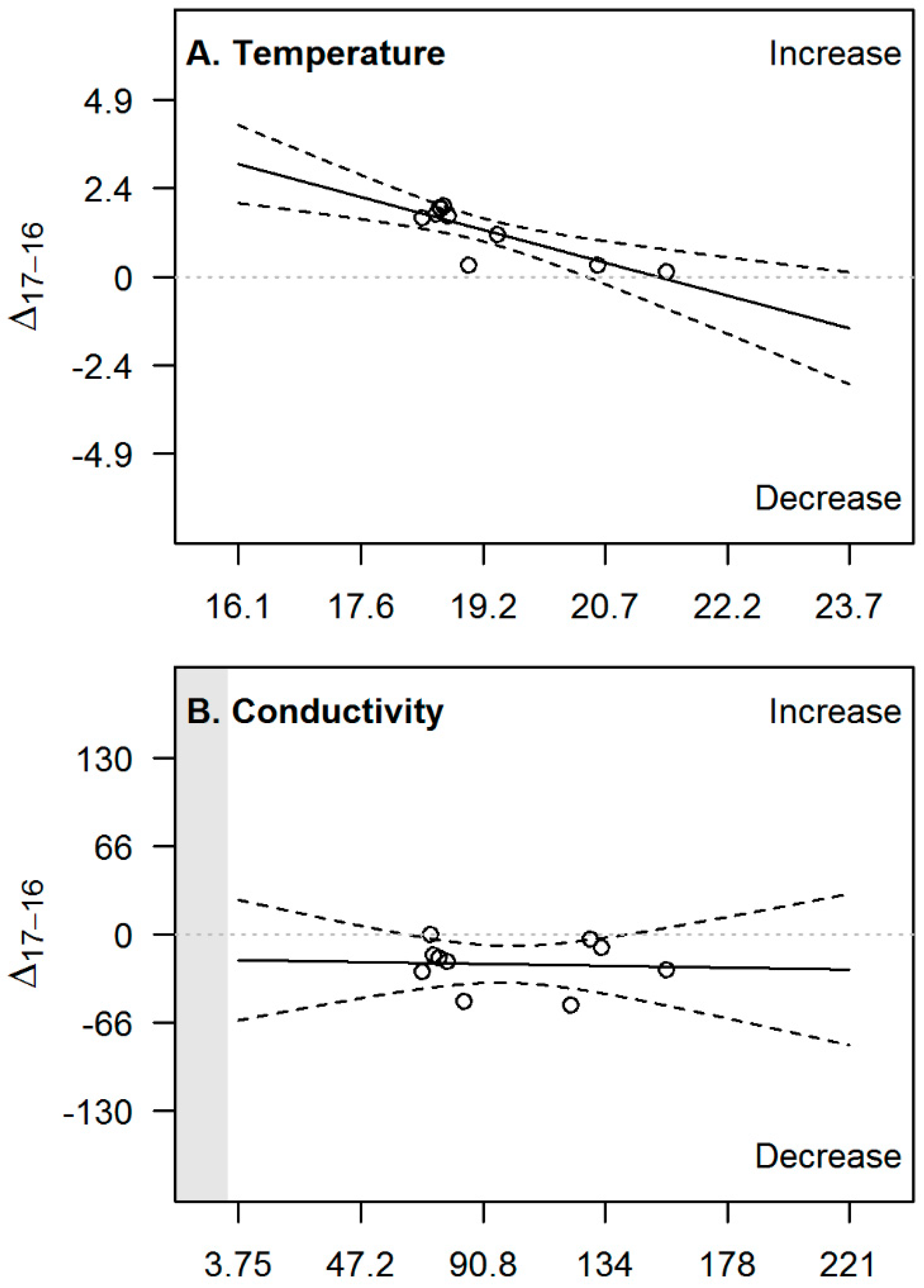
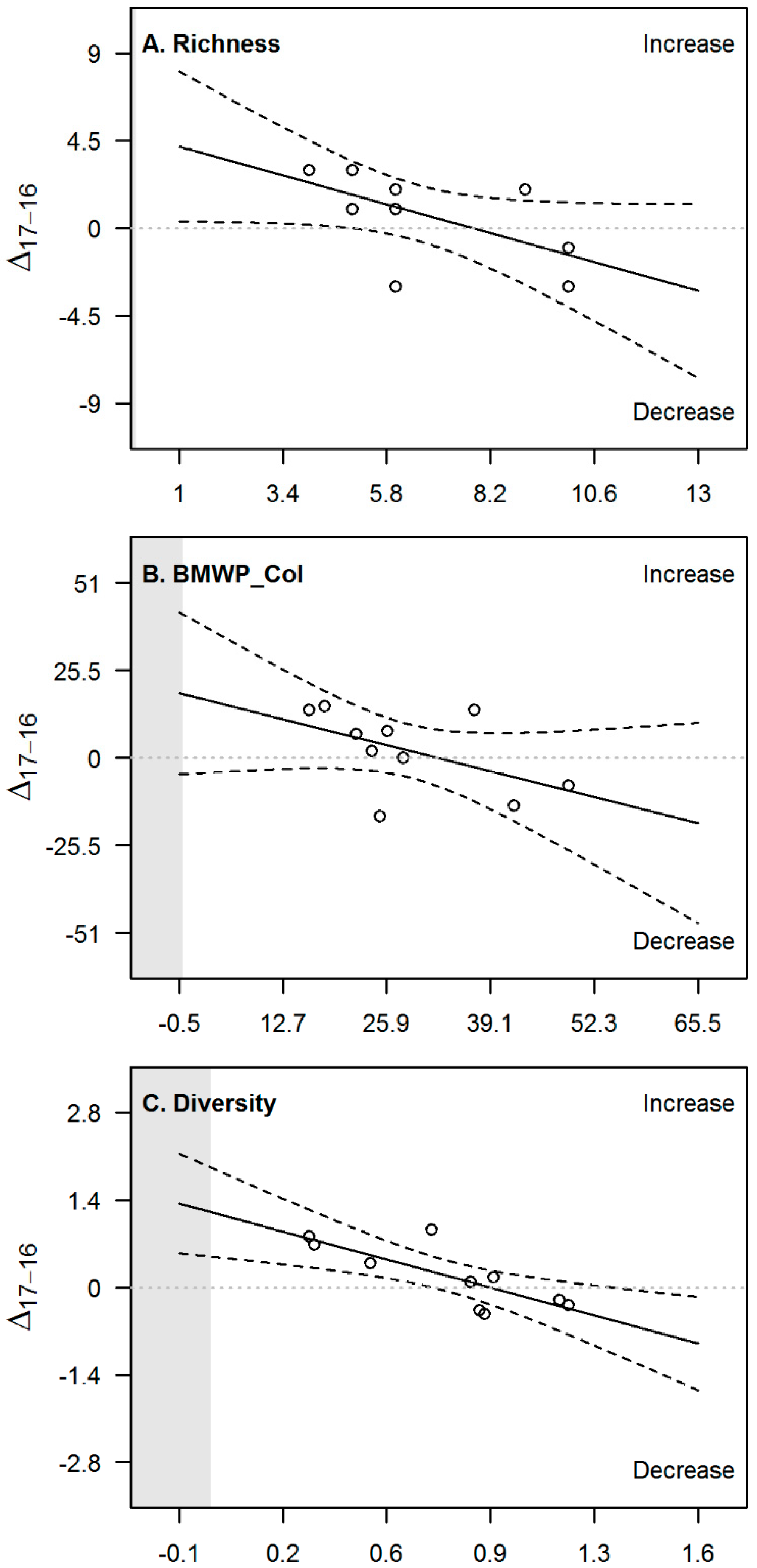
| Variable | Slope | p-Value | R2 | CI 2.5% | CI 97.5% |
|---|---|---|---|---|---|
| pH | −0.49 *** | 0.00002 | 0.90 | −0.61 | −0.36 |
| Turbidity | −0.66 *** | 0.0005 | 0.79 | −0.93 | −0.38 |
| DO | 0.085 | 0.8 | 0.01 | −0.71 | 0.88 |
| Temperature | −0.59 ** | 0.003 | 0.68 | −0.92 | −0.26 |
| Conductivity | −0.032 | 0.9 | 0.00 | −0.48 | 0.42 |
| Richness | −0.62 | 0.06 | 0.37 | −1.30 | 0.03 |
| BMWP_Col | −0.57 | 0.1 | 0.27 | −1.30 | 0.19 |
| Diversity | −1.30 ** | 0.008 | 0.61 | −2.1 | −0.44 |
© 2019 by the authors. Licensee MDPI, Basel, Switzerland. This article is an open access article distributed under the terms and conditions of the Creative Commons Attribution (CC BY) license (http://creativecommons.org/licenses/by/4.0/).
Share and Cite
Van Echelpoel, W.; Forio, M.A.E.; Van der heyden, C.; Bermúdez, R.; Ho, L.; Rosado Moncayo, A.M.; Parra Narea, R.N.; Dominguez Granda, L.E.; Sanchez, D.; Goethals, P.L.M. Spatial Characteristics and Temporal Evolution of Chemical and Biological Freshwater Status as Baseline Assessment on the Tropical Island San Cristóbal (Galapagos, Ecuador). Water 2019, 11, 880. https://doi.org/10.3390/w11050880
Van Echelpoel W, Forio MAE, Van der heyden C, Bermúdez R, Ho L, Rosado Moncayo AM, Parra Narea RN, Dominguez Granda LE, Sanchez D, Goethals PLM. Spatial Characteristics and Temporal Evolution of Chemical and Biological Freshwater Status as Baseline Assessment on the Tropical Island San Cristóbal (Galapagos, Ecuador). Water. 2019; 11(5):880. https://doi.org/10.3390/w11050880
Chicago/Turabian StyleVan Echelpoel, Wout, Marie Anne Eurie Forio, Christine Van der heyden, Rafael Bermúdez, Long Ho, Andrea Mishell Rosado Moncayo, Rebeca Nathaly Parra Narea, Luis E. Dominguez Granda, Danny Sanchez, and Peter L. M. Goethals. 2019. "Spatial Characteristics and Temporal Evolution of Chemical and Biological Freshwater Status as Baseline Assessment on the Tropical Island San Cristóbal (Galapagos, Ecuador)" Water 11, no. 5: 880. https://doi.org/10.3390/w11050880