Water Footprint of Crops on Rhodes Island


Department of Spatial Planning and Development, Faculty of Engineering, Aristotle University of Thessaloniki, 54124 Thessaloniki, Greece
*
Author to whom correspondence should be addressed.
Water 2019, 11(5), 1084; https://doi.org/10.3390/w11051084
Submission received: 7 April 2019
/
Revised: 19 May 2019
/
Accepted: 21 May 2019
/
Published: 24 May 2019
(This article belongs to the Section Water Use and Scarcity)
Abstract
:The aim of this paper is to evaluate the water footprints (WFs) of all the main crops on Rhodes island at a municipal unit (MU) scale, as well as for the area of the island as a whole. WF estimations are made with a distinction of rainfed and irrigated crops, using CROPWAT 8.0. Rainfed crops and the drip irrigation method are predominant in the study area, which faces water scarcity issues. Furthermore, a reduction factor in plant coefficients is introduced, to adapt to the drip irrigation technique. From the findings obtained, useful conclusions are drawn regarding the most water-demanding crops, but also the type of their WF component (blue/green/gray). In all categories of crops, there are large fluctuations across MUs, mainly due to the different yields. Higher WF values occur for rainfed and irrigated olives, which constitute the predominant crop, followed by hard and soft wheat. WF is a useful indicator identifying which crops require improvement or restructuring in a study area, and quantifies the exact volumes of water, which is a useful element in the formulation of agricultural policy in the context of sustainable water resources management.
1. Introduction
Farmers determine the levels of blue water withdrawn through irrigation and green water consumption through the ways in which the rainwater is captured in crop and fodder production [1]. Farmers, as the initial part of the supply chain, can be informed and trained in order to adopt water-conserving irrigation technologies, soil improvement methods, the optimized use of pesticides or chemical fertilizers, and shifting water usage to more water-efficient crops according to the water scarcity of their area, by changing their cropping patterns [2]. According to Kauffman et al. [3], an increase of the green water quantity in agriculture procedures can be achieved with proper soil and water management (reduced erosion/surface runoff/soil evaporation), which leads to increased rainwater infiltration into the rootable soil (increased green water) and an increase of groundwater recharge through percolation (increasing the volume of blue water).
The water footprint (WF) is an environmental indicator that takes into account the total amount of direct and indirect freshwater consumed and polluted in the full supply chain [4]. WF can take into account geographical differences in water availability and capture water return flows and the indirect amount of virtual water [5], and incorporate them into marketable products for their production, leading to a more comprehensive water consumption analysis. The WF is a multidimensional indicator which does not simply refer to the water volume used, as is the case for the ‘virtual water content’ of a product, but also contains further spatial and temporal information that makes it explicit where the WF is located, what source of water is used, and when the water is used [4].
According to Turner [6], in the year 2000, agriculture accounted for 70% of water withdrawals and 93% of water consumption worldwide, where consumption refers to the withdrawal net of return flows and evaporation. By estimating the blue-water component (irrigation) in agricultural production activities, approaches can be identified to reduce its consumption, while the proper management of green water (rainfall) consumed in agricultural processes leads to greater amounts of available rainwater to support natural vegetation and biodiversity. According to Falkenmark and Rockström [7], global food production consumes around 6800 km3 year−1 worldwide (as green water flow through evapotranspiration). Of this amount, 1800 km3 year−1 are consumed through the distribution of water in blue waters (return to rivers, lakes, and underground reserves) in irrigated crop production, while the remaining 5000 km3 year−1 represents the consumption of green water in global rainfed farming, which is applied to 80% of agricultural land.
According to the Water Framework Directive (WFD) [8], the river basin is considered the appropriate scale regarding water resources management; however, Hoekstra [9] argues that many water problems are extended beyond local levels and are linked to international trade. According to Hoekstra et al. [4], WF can be estimated at multiple levels, such as river basins; municipalities; provinces; or other administrative units, products, consumers, businesses etc. WF projects within geographical delineated areas have been performed at administrative unit and river basin levels [10]. Several studies have examined the WF of several crops at multiple scales [11,12,13,14,15,16,17,18,19]. WF studies have been conducted at a regional [13,16,20,21], national [22], and river basin scale [15,19]. Hoekstra and Hung [23] quantified the volumes of virtual water related to international crop trade flows between nations in the period 1995–1999. Mekonnen and Hoekstra [24] rated green, blue, and gray WFs from 126 crops around the world for the period 1996–2005, with a high spatial resolution. In Greece, WF applications have implemented evolving agricultural products at both an administrative and river basin level [19,20,25]. Zoumides et al. [17] presented a spatiotemporal model that was used to assess the blue and green WF of crop production in Cyprus for the period 1995–2009 and quantified the difference between the results of advanced global water use assessments, in order to compare global versus local crop WFs. Aldaya et al. [26] examined the strategic importance of green water in international crop trade and showed that the use of green water, which has a lower opportunity cost, for the production of crops generally has less negative environmental externalities than the use of blue water. According to Liu et al. [27], gray WF assessments have overwhelmingly been focused on N-related loads to freshwater and only a few studies have considered multiple pollutants, such as N, P, COD (chemical oxygen demand), and NH4 (ammonium).
Regarding the economic value of crops produced, Zoumides et al. [18] and Mellios et al. [19] examined the WF of crop production along with the economic perspective of trade in Cyprus (period 1995–2009) and exports in Greece, downscaled to the River Basin District (RBD) level, respectively. Zoumides et al. [18], in order to enhance the policy relevance of the WF, employed a supply use approach related to crop products along with two complementary indicators, namely the economic productivity of crop water use and a temporally explicit blue-water scarcity index. Mellios et al. [19] examined the exported virtual crop water per value ratio. Aldaya et al. [21] evaluated the WF of cotton, wheat, and rice in Central Asia using the CROPWAT model and included the concept of economic blue-water productivity to assess the production value, expressed as the market price per cubic meter of water, consumed when producing the commodity.
This study attempts to analyze the blue, green, and gray WFs of all the main crops on Rhodes island, with a separation of rainfed and irrigated ones, for the period 2000–2014 and per municipal unit (MU) for the year 2013. Calculations for a wide range of crops and per growing season (summer potato/spring/winter) and more specifically for all the main crops in the study area are performed in a small-scale region (Rhodes), where administrative and RBD boundaries are identical due to the island’s status. Green water consumption significance is emphasized in the study area, where, due to water scarcity issues, rainfed crops and the drip irrigation method are predominant. Moreover, a reduction factor is introduced in the plant coefficients, which are incoming data in the CROPWAT software (Land and Water Development Division of FAO, Rome, Italy) used for simulations, to adapt the drip irrigation technique. Soil characteristics include the influence of mechanical soil composition and soil organic matter and take into account further separation into a similar soil category (loam). The gray WF, which is widely evaluated for the pollutant nitrogen (N) and less commonly for phosphate (P2O5), includes further examination for the pollutant potassium (K) applied to the field by fertilization. Furthermore, a sensitivity analysis is performed, to examine the effect of a and cnat values on the gray WF estimations and kc fluctuations in a range of ±15%, to investigate blue and green WF variations.
2. Materials and Methods
2.1. Study Area and Data Sources
Rhodes administratively belongs to the South Aegean region and is considered a distinct river basin of the RBD of the Aegean Islands. As a requirement of the Water Framework Directive by Government Gazette 2019/17.9.2015, the River Basin Management Plan of the RBD of the Aegean Islands was approved, and with the Government Gazette (GG) B 4677/29.12.2017, the RBMP GR 14-Water Department of the Aegean has been updated. According to the River Basin Management Plan of the Aegean Sea, the Aegean islands have been experiencing water scarcity for three decades, mainly on the smaller islands and extending to the larger ones. Rhodes had a population of 115,490 in 2011, according to the Hellenic Statistical Authority (ELSTAT) [28], while in 2001 and 1991, it had a population of 115,334 and 96,159 inhabitants, respectively. Rhodes is the largest island in the Dodecanese and the fourth largest in Greece after Crete, Evia, and Lesvos. The study area spreads over an area of 1398 km2 and its shape is oblong, with a maximum length of 77 km and a maximum width of 37 km. Administratively, the municipality of Rhodes is subdivided into the following MUs: Rhodes, Archangelos, Atavyros, Afantou, Ialysos, Kallithea, Kameiros, Lindos, South Rhodes, and Petaloudes.
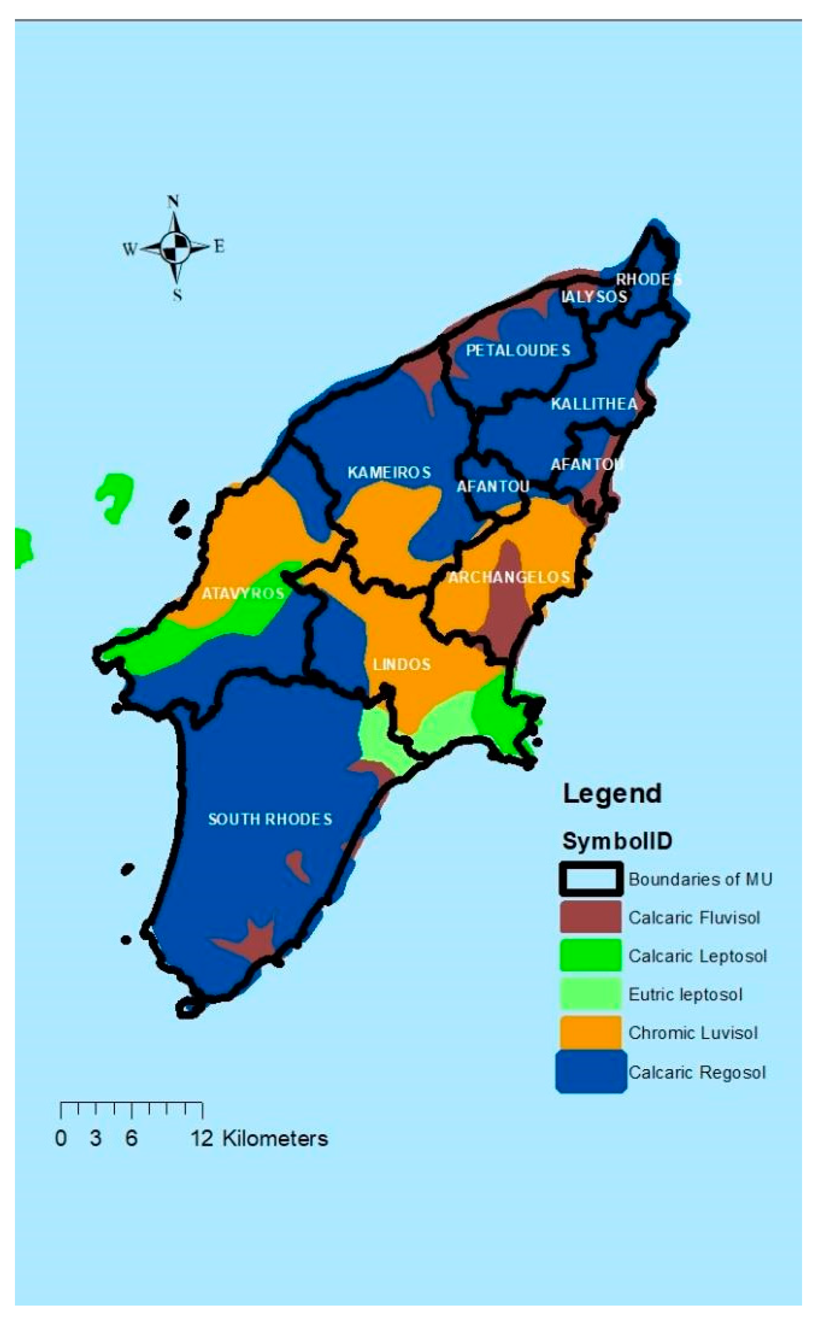
Figure 1 depicts the main categories of soils found on the island of Rhodes due to the international soil classification system ‘The World Reference Database (WRB)’, obtained from the European Soil Data Centre [29]. As the study area includes soils of the same class, an additional separation into soils was performed according to their mechanical composition. Mechanical soil composition properties were calculated from the ‘Harmonized World Soil Database Viewer Version 1.2’ [30], while the soil’s hydraulic properties were calculated with the Soil Water Characteristics software, which is included in the United States Department of Agriculture (USDA) ‘Spaw Hydrology’ model [31]. The map of the MU of Rhodes island was obtained from ‘AEGIS: a wildfire prevention and management information system’ [32]. In Figure 1, the predominant soils at an MU resolution are presented. In computations of the WFs per crop according to their distribution, four main categories of soils were considered: Calcaric Fluvisols, Calcaric Leptosols, Chromic Luvilos, and Calcaric Regosols (Eutric and Calcaric Leptosols have similar features).
The distribution of agricultural land was taken based on CORINE Land Cover 2012 [33]. Agricultural data of croplands and crop production were taken from ELSTAT (annual agricultural statistics). For crops with no high-resolution maps, data were obtained from the “Escalation maps of cultivation in Greece”, of the Ministry of Rural Development and Food. The study examines the WF of the following crops: irrigated/rainfed olives, citrus, irrigated grapes/rainfed grapes, vegetables, irrigated/rainfed rest annual crops (only for the year 2013), melons, spring/summer/winter potatoes, soft/hard wheat, barley, and fodder crops. According to the analytical harvested area of crops as derived from the processing of ELSTAT data of the year 2013, the most widespread crop on the island of Rhodes is the olive groves (67%), followed by hard wheat (8%) and fodder crops (6%) [28]. The estimation methodology involves a spatial analysis that uses the ARCMap software (Environmental Systems Research Institute, Redlands, CA USA) through the formation of new layers, including combined information of soil characteristics per crop and per MU.
For the estimation of WFs, crops were divided into those that are rainfed and irrigated, taking into account ELSTAT data and according to the Directorate General of Regional Agricultural Economy and Veterinary of the Region of South Aegean. The most prevalent crop on the island is that of rainfed olive trees, with the largest area in the MU of Archangel MU, while the second most prevalent is hard wheat, with the largest area in the MU of South Rhodes.
Meteorological data for the period 2000–2014 at a monthly resolution were obtained from the meteorological station of the Hellenic National Meteorological Service (HNMS), which is based in the MU of Rhodes. Based on climatic data, the CROPWAT 8.0 [34] software calculated the reference evapotranspiration (ETo) with the FAO Penman-Monteith method [35].
The analysis was performed by calculating the WFs of the catchment area of Rhodes as a whole for the period 2000–2014 (due to recent data availability) and per MU for 2013 (due to the availability of data and CORINE Land Cover 2012 proximity).
The gray WF refers to the volume of water needed to dilute a certain amount of pollution such that it meets ambient water quality standards or is equivalent to natural background concentrations [4]. WF (for the pollutants of nitrogen (N), phosphate (P2O5), and potassium (K) applied to the field by fertilization) was obtained based on the Greek Ministerial Decision No 38295/2007 concerning “Quality of water for human consumption”. The maximum permitted value for nitrate ions (NO3) is 50 mg L−1, which is equivalent to 11.3 mg L−1; as nitrate-nitrogen (NO3-N), following Chapagain et al. [36]. The calculation was made by considering nitrate-nitrogen, as nitrate is one part nitrogen plus three parts oxygen, with nitrogen accounting for only 22.6% of the nitrate ion.
Due to limited surface adsorbents (mainly streams) and surface runoff rates of the applied quantity, according to the first revision of the RBMP GR 14-Water Department of the Aegean, (GG B 4677/29.12.2017), the gray WF for surface systems is considered to be negligible and the calculations concern underground water systems.
Natural concentration (cnat) in a receiving water body is the concentration in the water body that would occur if there were no human disturbances in the catchment [4]. Data for the natural concentration (cnat) of pollutants were received according to the Government Gazette (GG) B 4677/29.12.2017 (RBMP GR 14-Water Department of the Aegean) and from the bibliography according to Chapman [37]. The amount of pollutant WF concerns the amount of pollutants of nitrogen (N), phosphate (P2O5), and potassium (K) applied to the field by fertilization. The quantities of recommended fertilization per crop type and the fertilizer absorption rates (with a value range of 80–90%, depending on the crop) were derived from the Government Gazette 2019/17.9.2015 (the River Basin Management Plan of the RBD of the Aegean Islands).
2.2. Methodology
Through the calculation framework developed by Hoekstra et al. [4], the total WFs of crops were calculated as the sum of the three components of green (Equation (1)), blue (Equation (2)), and gray (Equation (3)) water consumption. The aforementioned methodology was chosen because it is a widespread standalone approach that provides volumetric WFs considering the three water volume components (blue, green, and gray) in terms of water resources management. The estimations were performed following a combination methodology of excel spreadsheets, ARCMap [38] software (new layers of spatial units were created from the layers of land uses and geological backgrounds), and CROPWAT 8.0 simulation software. The aforementioned simulation software, used to estimate the water consumption of crops on the island, is a high-reliability program developed by the Food and Agriculture Organization of the United Nations (FAO) and widely used for many years [39,40,41,42]. The ‘irrigation schedule CROPWAT option’ is used in order to calculate the actual evapotranspiration, which instead of taking into account effective precipitation, includes a soil water balance which keeps track of the soil moisture content over time using a daily time step, employing incoming monthly climate data in WF calculations. The four basic input data categories to CROPWAT are related to climate, rainfall, soil type, and crop characteristics.
To adapt to drip irrigation, which is mostly applied to the study area, a reduction factor was introduced in the process of calculating single plant coefficients (Equation (8)), as incoming data of CROPWAT 8.0. In addition, plant coefficients (kc) and the critical depletion fraction (p) were adapted to the climatic data of the study area, taking into account each plant growing season climate (Equations (8) and (9)).
The calculation of the green WF of a crop applies as follows [4]:
where CWUgreen is the green water used per unit area of a crop (m3 ha−1) and Y is the crop yield (t ha−1).
The green water consumed during the crop growth expresses the contribution of rainfall required to cover the water needs of each crop. CWUgreen is determined by the evapotranspiration requirements at all stages of plant growth, taking into account available soil moisture.
The blue WF can be estimated by reference [4]
where CWUblue is the volume of blue water used per unit of cultivation (m3 ha−1) and Y is the yield of the crop (t ha−1).
The gray water refers to the theoretical volume of water required to dilute the pollution load resulting from the use of agrochemicals [4]. Gray WF is only considered for the most polluting component (critical pollutant: WFgray = MAX from WFgray(P2O5); WFgray(N); WFgray(K), as the volume of water required to reduce the concentration of the critical pollutant to permissible levels is sufficient to dissolve the other pollutants) and can be derived according to the following Equation (4):
where a is the percentage of pollutant entering the system (%), AR is the amount of pollutant used per unit area of a crop (kg ha−1), cmax is the maximum permissible concentration of the pollutant per unit volume of water (kg m−3), cnat is the natural concentration of the pollutant per unit volume of water (kg m−3), and Y is the crop yield (t ha−1).
The calculation of reference evaporation (ETo) was derived from the F.A.O. Penman–Monteith method, given by the following relationship [35]:
where ETo is the reference evapotranspiration (mm day−1), Rn is the net radiation at the crop surface (equivalent radiation in mega joules per square meter per day: MJ m−2 day−1), G is the soil heat flux density (MJ m−2 day−1), T is the mean daily air temperature at a 2 m height (°C), u2 is the wind speed at a 2 m height (m s−1), es is the saturation vapor pressure (kPa), ea is the actual vapor pressure (kPa), es−ea is the saturation vapor pressure deficit (kPa), ∆ is the slope vapor pressure curve (kPa °C−1), and γ is the psychrometric constant (kPa °C−1).
Equation (5) [35] was used for the adjustment of wind speed data to the height of 2 m above the ground surface:
where u2 is the wind speed 2 m above the ground surface (m s−1), uz is the wind speed measured z m above the ground surface (m s−1), and z is the height of measurement above the ground surface (m) [35].
where ETc is the crop evapotranspiration (mm day−1), kc is the crop coefficient [dimensionless], and ETo is the reference crop evapotranspiration (mm day−1).
According to Allen et al. [35], the calculation of actual evaporation (ETa—evapotranspiration in non-ideal conditions) is calculated according to Equation (7):
where ETa is the actual evapotranspiration (mm day−1), ETo is the evaporation of the reference crop (mm day−1), kc is the crop coefficient [dimensionless], and ks is the coefficient referring to the soil moisture status or other factors (such us soil salinity) with values of 0 < ks ≤ 1.
Plant kc values, as well as the duration of the four growth phases for each crop, were obtained from Papazafeiriou [43] and from the FAO technical datasheet [35]. Incoming data to CROPWAT concerning the root depth (RD) with a differentiation among rainfed and irrigated conditions, critical depletion fraction (p), yield response factor (ky), and crop height were derived from the CROPWAT software libraries and from the FAO-56 tables [32]. The critical depletion fraction for every crop was readjusted depending on the ETC evapotranspiration for each crop growth stage, following FAO-56 [35].
In addition, plant coefficients kc,mid and kc,end were also adapted to the climatic data of the study area, taking into account each plant growing season climate and each year separately, as the values given by Allen et al. [35] refer to climate with a mean RHmin of 45% and wind speed of 2 m s−1. The readjustment was made according to the following relationship:
where kc(TAB) is the value for kc,mid and kc,end (when ≥ 0.45) taken from the tables of FAO-56 [35]; u2 is the mean value for daily wind speed at a 2 m height over grass, during the late season or mid-season growth stage (m s−1), for 1 m s−1 ≤ u2 ≤ 6 m s−1; RHmin is the mean value for daily minimum relative humidity during the late or mid-season stage (%), for 20% ≤ RHmin ≤ 80%; and h is the mean plant height during the late or mid-season stage (m), for 0.1 m ≤ h.
As mentioned above, due to the adaptation of the simulation software required to calculate the evapotranspiration for the drip irrigation method and in order to take account of the reduction in evaporation for this irrigation method, the planting factors for irrigated crops were adjusted, taking into account the reduction factor against Papazaferiou [44], according to which
where ETt is the evapotranspiration under drip irrigation conditions, ET is the evaporation diffusion calculated by various methods, and Pc is the percentage of the area covered by the projection on the soil of the foliage of the crop.
The coverage of soil according to the crops and the stages of their development were taken according to Papazafeiriou [44]. Considering the aforementioned approach (Equation (9)) for the drip irrigation method, the plant coefficients as incoming data in the simulation software for all irrigated crops were adjusted as a function of the specific irrigation technique used, expressed as the following equation:
Finally, according to the ‘irrigation schedule’ approach of CROPWAT and the Water Footprint Manual [4], Equations (11) (rainfed conditions), (12) and (13) (irrigated conditions) were used, where the total water evapotranspired (ETa) over the growing period was equal to what is called the ‘actual water use by crop’ in the CROPWAT. The green water evapotranspiration (ETgreen), the blue-water evapotranspiration (ETblue), and the total evapotranspiration, (ETa) were estimated based on the software outputs. For rainfed conditions, the following was applied:
For irrigated conditions, the following was applied:
ETblue = min (total net irrigation/actual irrigation requirement).
3. Results
3.1. WFs per MU for 2013
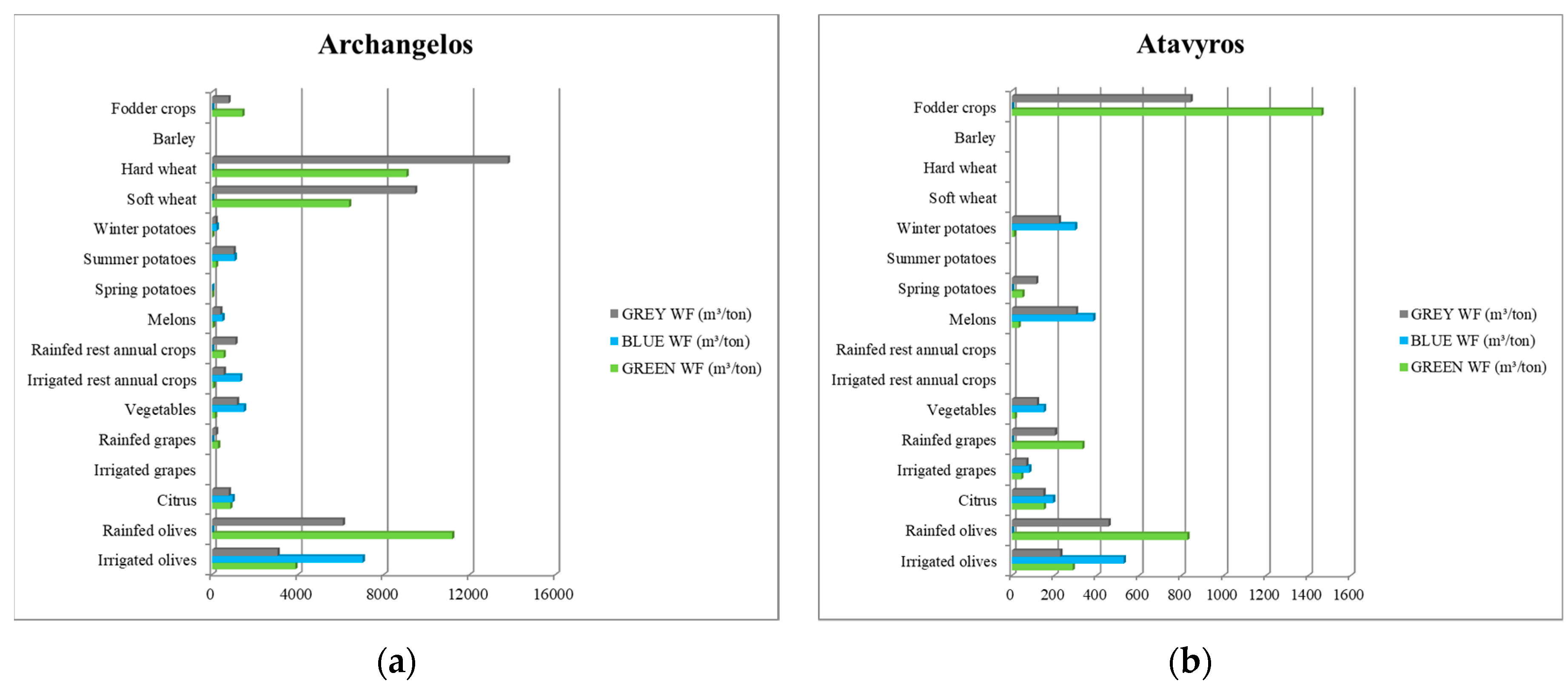
From the results obtained per MU, for the WF of the crops in m3 t−1, useful conclusions are drawn regarding the most demanding plantations, but also the type of water requirement (blue, green, and gray). Indicatively, the results obtained for Archangel and Atavyros MUs are presented in Figure 2. At the first aforementioned MU, the most demanding crops concerning green water use (m3 t−1) are rainfed olive trees and wheat (soft and hard), while regarding blue water use (m3 t−1), irrigated olive trees are the most consuming crops.
As depicted in Figure 2b in the MU of Atavyros, it is evident that the most demanding cultivation in green water use refers to fodder crops, followed by the rainfed olives, while in blue use, the most demanding are the irrigated olives, melons, and winter potatoes. In general, the resulting image at each MU differs, mainly depending on the type of prevailing crops and their respective yields.
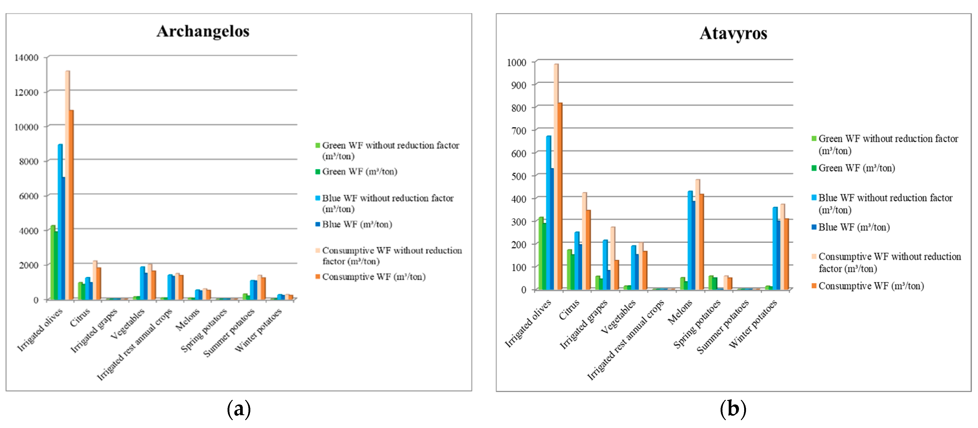
In Figure 3a,b, blue, green, and consumptive WFs in m3 t−1 are presented indicatively for the MUs of Archangelos and Atavyros, considering the calculations for the irrigated crops, with and without the inclusion of the reduction factor (Equation (14)) in the plant coefficients, in order to compare WF values.
Irrigated crops’ WFs in all MUs present higher values when the reduction factor is not included in the calculation of crop coefficients, with the scope of drip irrigation conditions adaptation. From the comparison of the prices, consumptive WFs in all cultures (apart from grapes, which have larger deviations, due to lighter foliage shading) show variations of 5–25%, while in blue WF, variations range from 5–30%. These fluctuations mainly depend on the percentage of foliage shading of the plantation, as in the tree crops, such as olive and citrus trees, it is consistently high throughout the growing season, while in the annual crops, it is differentiated by the vegetative growth stage.
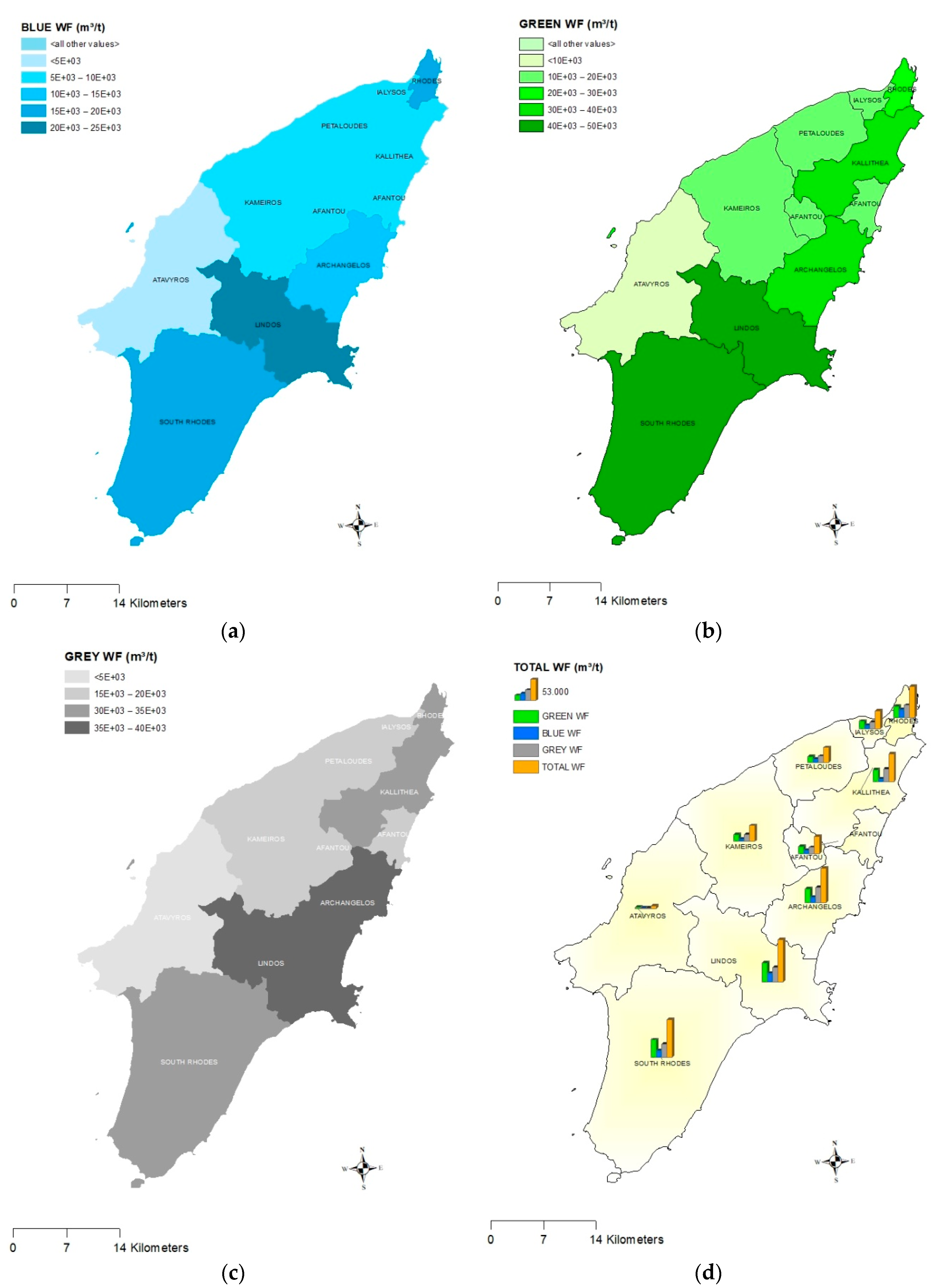
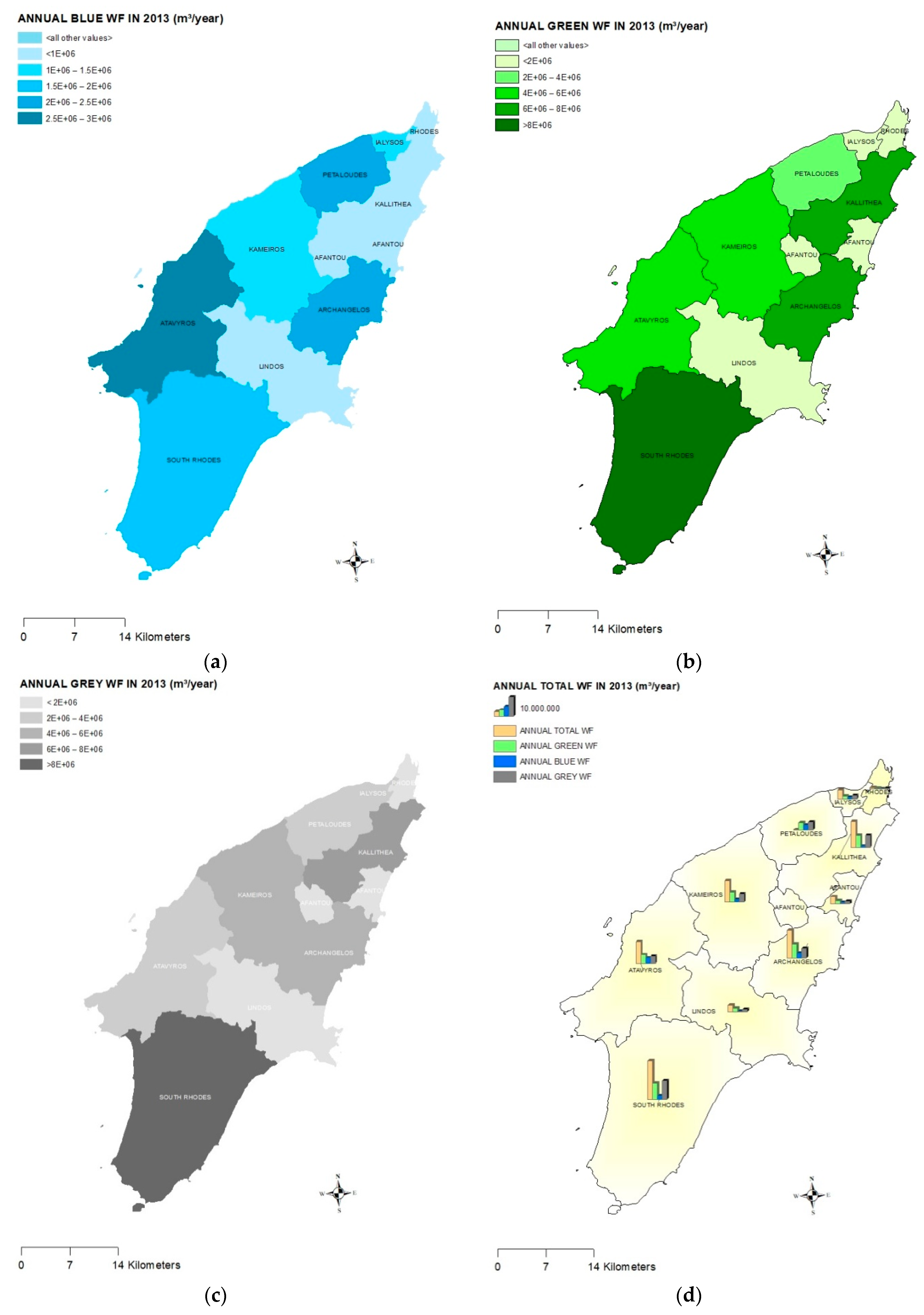
In the following Figure 4 and Figure 5, the green, blue, gray, and total WFs (m3 t−1) and the annual green, blue, gray, and total WFs (m3 year−1) for the year 2013 per MU are depicted, respectively. It is clear from Figure 4 and Figure 5 that the values of WFs in each MU differ, mainly depending on the type of prevailing crops and their respective yields.
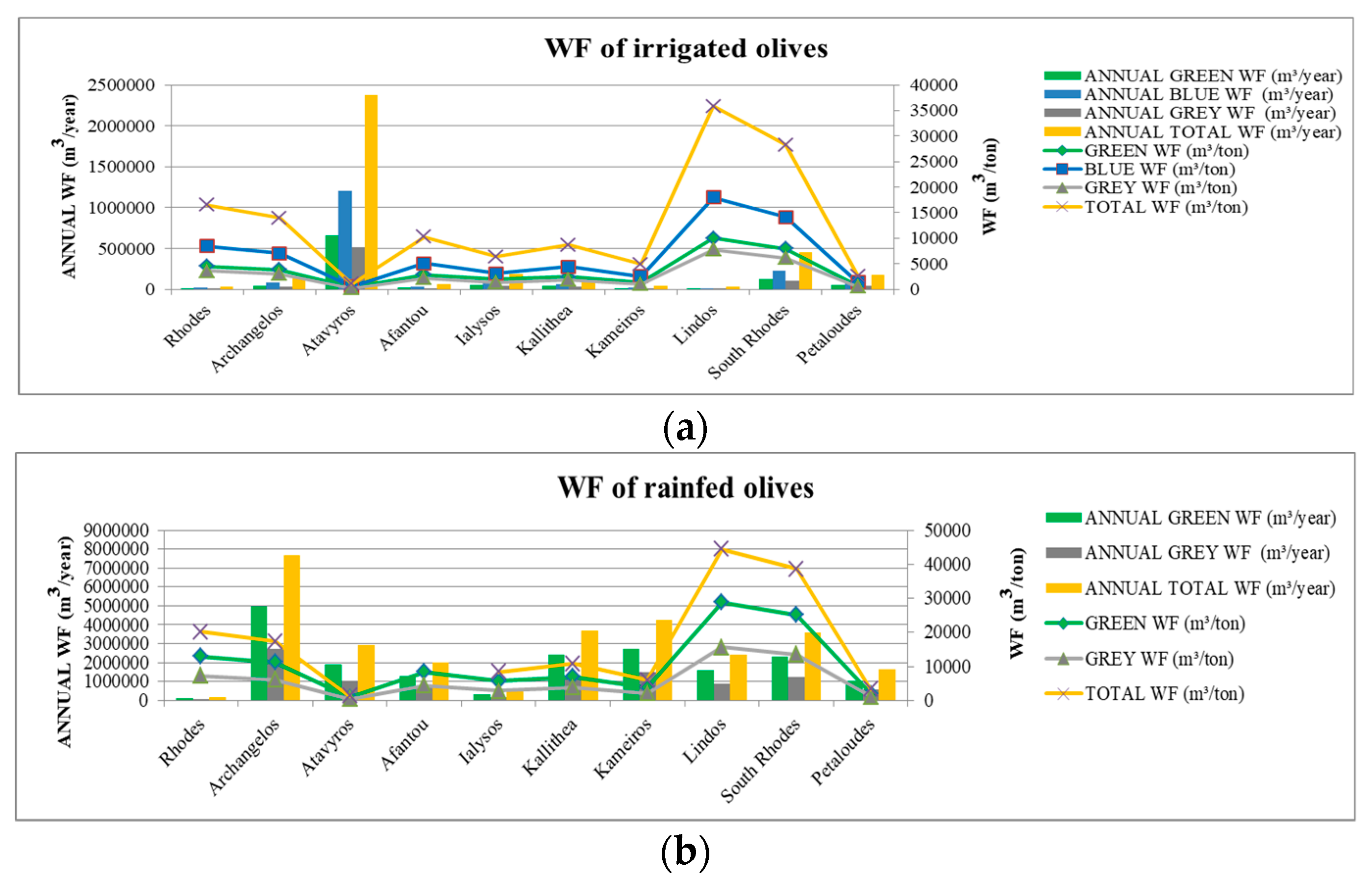
As presented in Figure 6a, for the cultivation of irrigated olive groves, the largest blue, green, gray, and total annual WF (m3 year−1) is shown in Atavyros, while the largest blue, green, gray, and total WF m3 t−1 is shown in Lindos. In Figure 8b, regarding the cultivation of rainfed olive groves, the largest green, gray, and total annual WF (m3 year−1) is depicted in Archangelos, while the largest green, gray, and total WF (m3 t−1) is shown in Lindos.
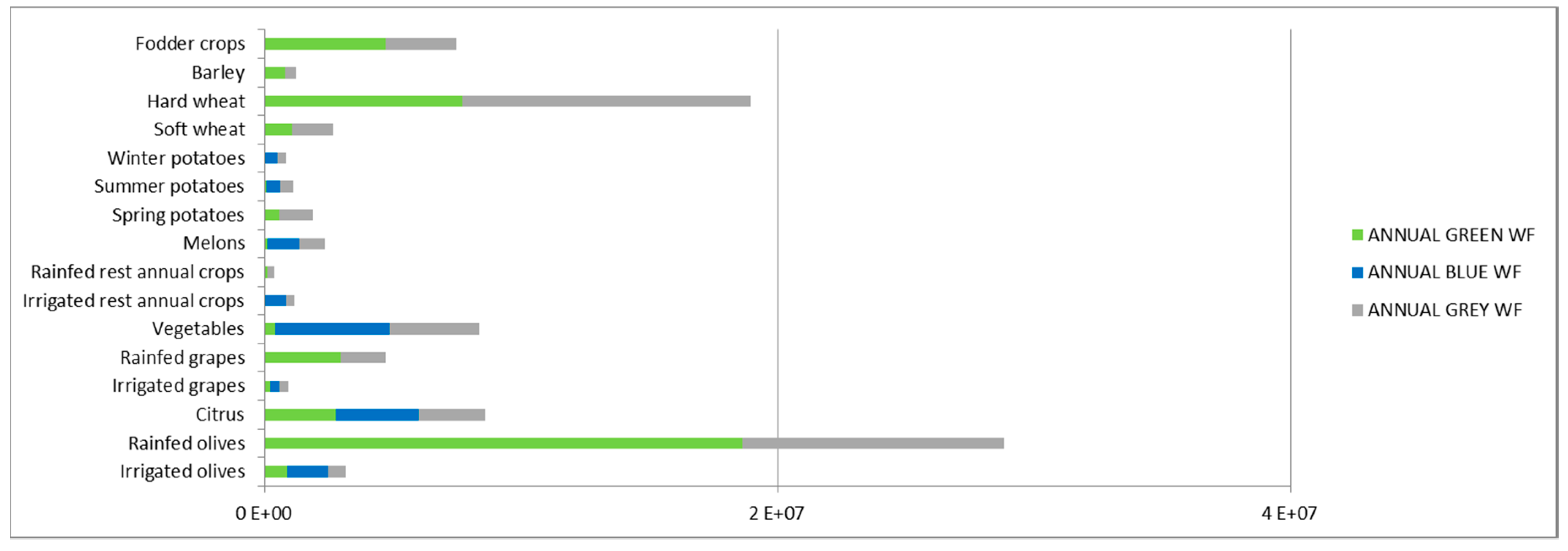
In Figure 7, the total annual blue, green, and gray WF (m3 year−1) for the Rhodes island per crop is presented. The largest total annual WF concerns rainfed olives, followed by hard wheat, fodder crops, vegetables, citrus, and rainfed grapes. The larger blue, green, and gray WF appears in vegetables, rainfed olive trees, and hard wheat, respectively.
The total annual consumption of the most common crops on the island of Rhodes for the year 2013 is estimated to be 13 MCM year−1 (blue component of WF) and 41 MCM year−1 (green component of WF), while the gray WF component is equal to 39 MCM year−1. The annual WF of crops calculated as the sum of the three components has a value of 93 MCM year−1.
3.2. Sensitivity Analysis
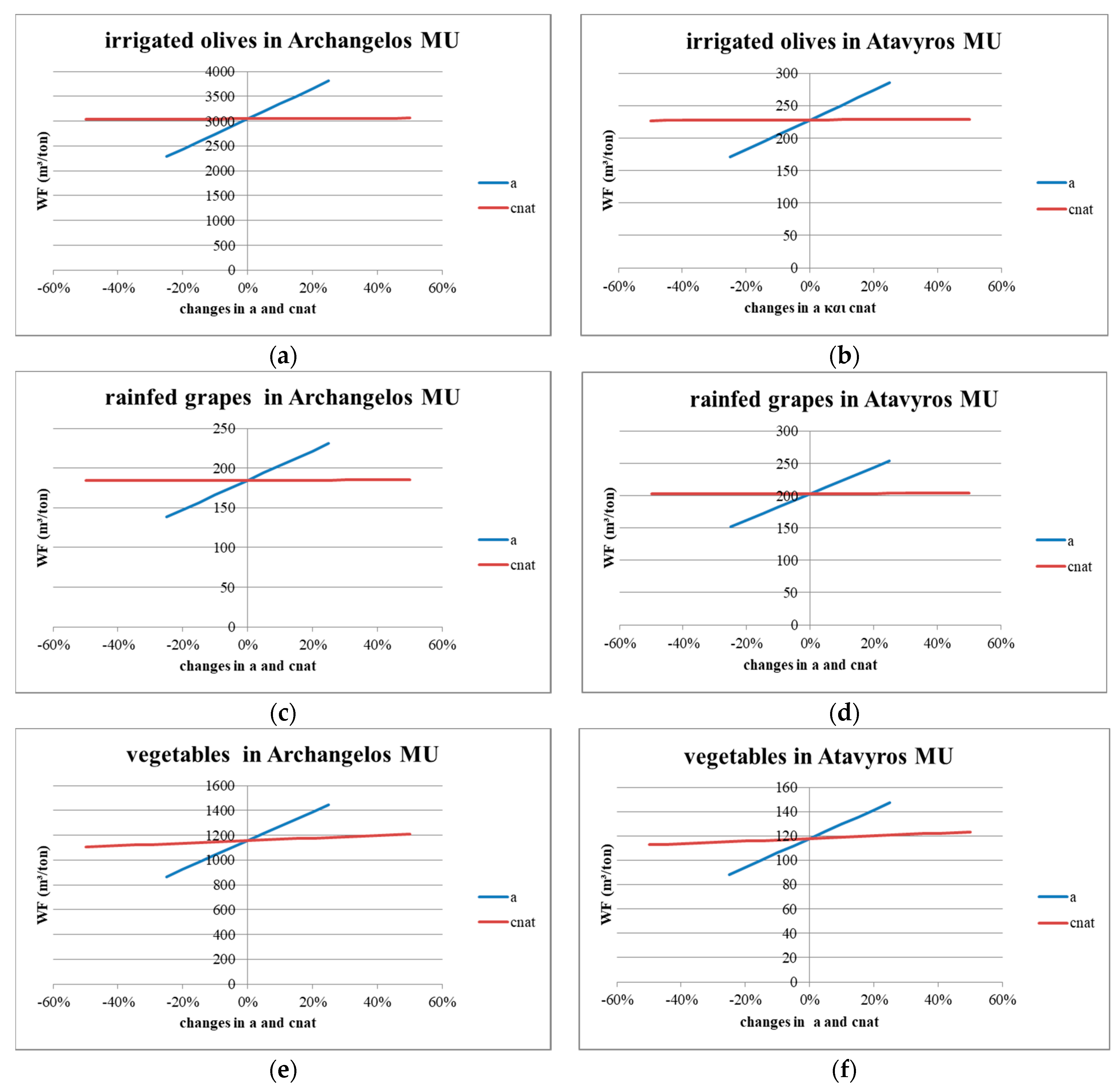
A sensitivity analysis was performed (i) to examine the effect of a and cnat values of Equation (3) on the gray WF estimations and (ii) to investigate the variability of kc in green and blue WFs. More specifically, keeping the other factors of Equation (3) constant, the gray WF for all the examined crops was re-calculated in each MU, with a fluctuation of ± 50% and ±25% in the cnat value and a value, respectively. The aforementioned variations have been taken in a manner that ranges in reasonable suspects, in accordance with the Government Gazette (GG) B 4677/29.12.2017, (RBMP GR 14-Water Department of the Aegean). According to Jagtap and Jones [45], the kc value for a certain crop can vary by 15% and following Zhuo et al. [15], with the adoption of this value, a sensitivity analysis can be performed considering kc values in a range of ±15% in order to investigate blue and green WF variations.
In Figure 8, indicative MUs of Archangelos and Atavyros are presented, regarding the irrigated olives, rainfed grapes, and vegetables. Gray WF results of the sensitivity analysis were assessed for the variability of a and cnat for every MU of the year 2013. The aforementioned crops are indicatively represented for the critical pollutant of nitrogen (N) for irrigated olives’ gray WF (Figure 8a,b), while critical pollutants of phosphate (P2O5) and potassium (K) refer to cultivations of rainfed grapes (Figure 8c,d) and vegetables (Figure 8e,f), respectively. According to Equation (3), variations of A and AR values directly and proportionally affect the gray WF, while the sensitivity analysis shows that the variability of gray water is more sensitive to a value compared with the cnat factor. Moreover, WF is more sensitive in cnat fluctuation when the critical pollutant is potassium (K) compared to the pollutants of nitrogen (N) and phosphate (P2O5).
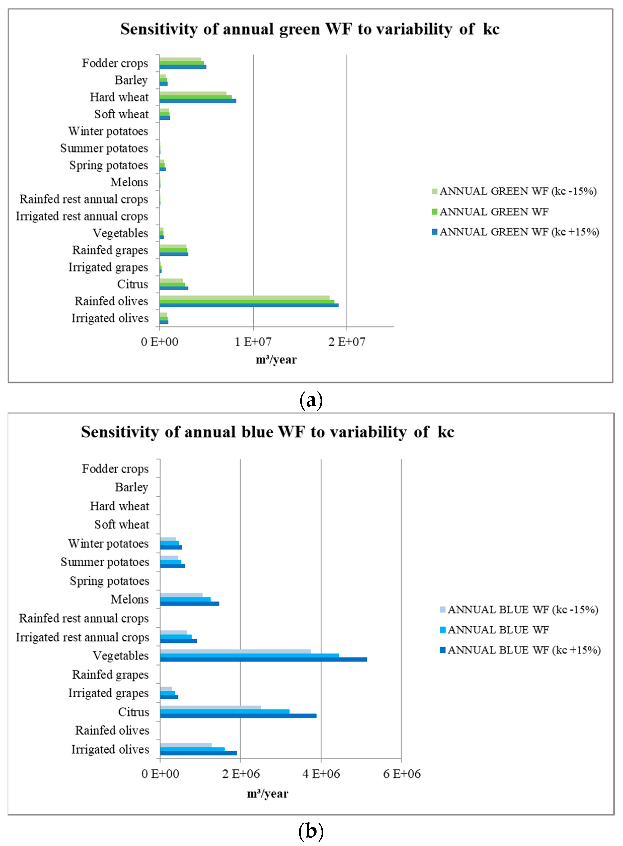
The sensitivity of annual green and blue WFs (m3 year−1) to ±15% variability of the kc input in CROPWAT WF estimations is presented in Figure 9a,b, respectively.
According to the sensitivity analysis performed, the total annual consumption of the most common crops on the island of Rhodes for the year 2013 regarding kc fluctuation of +15%/−15% is estimated to be 13 (+2/−3) MCM year−1 (blue component of WF) and 41 ± 2 MCM year−1 (green component of WF), while the gray WF component equals 39 ± 10 MCM year−1. The annual WF of crops calculated as the sum of the three components has a value of 93 (+14/−15) MCM year−1.
3.3. WFs for the Period 2000–2014
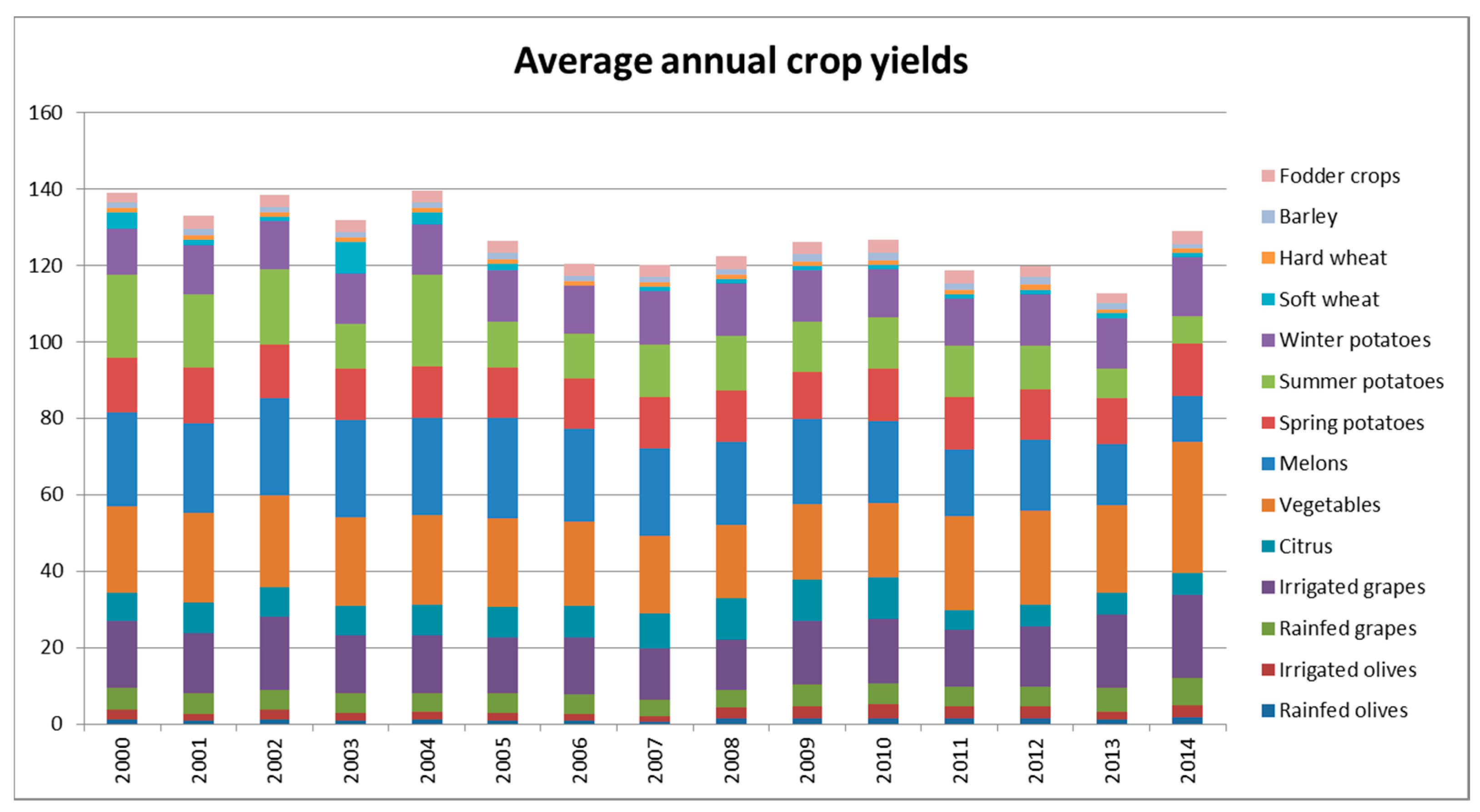
After processing ELSTAT data as presented in Figure 10, crops with large fluctuations in yields per year are mainly summer potatoes, fodder crops, and vegetables. The crops of vegetables, fodder, irrigated grapes, and potatoes exhibit the highest yields, while lower yields are mostly related to the non-irrigated crops.
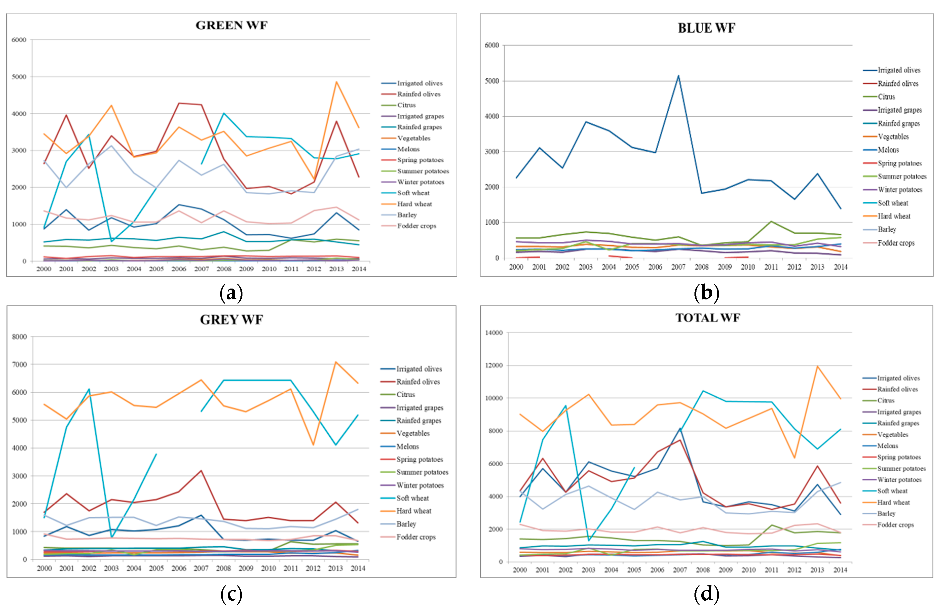
In the following Figure 11a,b,d, the results of all WF components (blue, green, and gray) in m3 t−1 are depicted for all crops, broken down into irrigated and rainfed ones for each separate year of the period 2000–2014.
More specifically, Figure 11a presents green WFs (m3 t−1) for all irrigated and rainfed crops, with larger values for the crops of hard and soft wheat, rainfed olives, barley, and rainfed grapes. In general, rainfed crops tend to exhibit larger green WFs compared to irrigated ones, mainly due to their smaller yields.
In Figure 11b, blue WFs (m3 t−1) are shown for all irrigated crops over the period 2000–2014 and it is obvious that the highest values and fluctuations concern the cultivation of irrigated olives, while the rest of the crops are below the value of 1000 m3 t−1 for all years.
The highest values of gray WF (m3 t−1) (Figure 11c) are related to the crops of hard and soft wheat, followed by crops of rainfed olive trees, barley, and rainfed grapes. Generally, rainfed crops present higher grey WFs compared to irrigated ones, mainly due to their small yields.
4. Discussion
From the results of the WF of the crops in m3 t−1 obtained per MU, useful conclusions are drawn regarding the most water-demanding crops, but also the type of water requirement. The WF of crops production exhibit significant differences on the MU level, mainly due to the different yields. There is a strong spatial dependence and heterogeneity in the distribution of the WF per MU.
WFs of rainfed and irrigated olives, which are the most widespread crops grown throughout the study area, prevail as higher values, followed by hard and soft wheat. In addition, significant differences appear between WFs of rainfed and irrigated crops.
In the irrigated crops of vegetables, melons, and winter potatoes, a very small green WF in relation to blue is observed, which reveals their high demand for irrigation water. Potatoes are cultivated in three different periods and depending on the different climates of each period, there is a significant difference between their green and blue WFs. Spring potatoes with greater green water availability show up zero blue WFs, while the reverse happens with the autumn and winter potatoes. In general, it is noted that green and grey WFs range at higher levels throughout the island, compared to blue WFs.
The maps of annual WFs (m3 year−1) indirectly indicate the crop production levels in tonnes per MU, but also depend on the levels of WF (m3 t−1) of the crops concerned. Therefore, an MU can exhibit small WFs (m3 t−1) because crops that are widespread in the area have low water requirements and/or high yields and have a high water consumption per year (m3 year−1) due to high production and/or vice versa.
The total annual consumption of the most common crops on the island of Rhodes for the year 2013 is estimated to be 13 MCM year−1 (blue component of WF) and 41 MCM year−1 (green component of WF), while the grey WF component equals 39 MCM year−1. The annual WF of crops calculated as the sum of the three components has a value of 93 MCM year−1.
Considering WF without the introduction of the reduction factor in irrigated crops for a comparison of the results, the total consumption of the blue component for the most common crops on the island of Rhodes for the year 2013 is estimated to be 14 MCM year−1 and that for the green component is 42 MCM year−1, and the gray balance is 39 MCM year−1. The total WF is equal to 95 MCM year−1, resulting in a deviation of 2 MCM year−1.
Crops with large fluctuations in yields per year are mainly summer potatoes, fodder crops, and vegetables. The crops of vegetables, fodder, irrigated grapes, and potatoes exhibit the highest yields, while lower yields are mostly related to the non-irrigated crops. The largest total WF is exhibited for the cultivation of hard wheat, followed by cultivations of soft wheat and olive trees (rainfed and irrigated), while larger values of consumption WFs (blue and green) concern the crops of irrigated olives followed by hard wheat, rainfed olives, soft wheat, and barley.
Through the analysis performed, evaluating the WF per MU for 2013 and WFs of Rhodes for the period 2000–2014, it is obvious that there is a variation in the values both in space and time. Yields vary considerably, even within the island, which significantly affects WF values.
According to Falkenmark and Rockström [7], there is an urgent need to focus on water investment in agricultural rainfed farming and this recognition requires the widening of current agricultural policy on water, which has been distorted for decades and only focuses on water for irrigation (blue component). In 2015, at an UN Summit, countries adopted the 2030 Agenda for Sustainable Development and its 17 Sustainable Development Goals, for the period 2015–2030 and according to Hoekstra et al. [46], goal 6 lacks any target on using green water more efficiently and on equitable sharing of water, even though the green water has more potential to be used productively in agriculture compared to blue-water resources. Green water use is often neglected because it has a lower opportunity cost than blue water [47]. According to Hess [48], the green water component of the WF of crops is important because it is helpful in the estimation of the total impact of crop production on the aquatic environment and the demonstration of the importance of rainfed agriculture on global agricultural production and food security, while it usually affects blue-water estimations and availability for other uses (such us domestic water supply or industry in a catchment).
The present investigation, distinguishing the rainfed from the irrigated crops and the WF into its components (blue, green, and gray water consumption), emphasizes the significance of green water, in an area where due to water scarcity, rainfed crops are very widespread. WF identifies which crops require improvement or restructuring in a study area and quantifies the exact volumes of water, which is a useful element in the formulation of agricultural policy in the context of sustainable water resources management.
Recently (in 2019), Hoekstra [49] proposed a generic and physically based method for green and blue water accounting in crop cultivation, in order to overcome ambiguities, such us the more accurate differentiating between green/blue water and their terminology, the distinction between E and T that stems from irrigation, and so on, in order to improve the estimation of irrigation water consumption, irrigation efficiency, and green and blue WFs in agriculture.
One limitation of the study regarding gray WF computation is that data for the natural concentration (cnat) of potassium were received from the bibliography according to Chapman [37] because the Government Gazette (GG) B 4677/29.12.2017 (RBMP GR 14-Water Department of the Aegean) only includes values for type-specific reference conditions for nitrogen and phosphate pollutants. Furthermore, due to the lack of real temporal and spatial data concerning the amount of pollutants of nitrogen, phosphate, and potassium applied to the field by fertilization of farmers, gray WF accounting is based on the recommended fertilization per crop type and the fertilizer absorption rates (with a value range of 80–90%, depending on the crop) from the Government Gazette 2019/17.9.2015 (the River Basin Management Plan of the RBD of the Aegean Islands). Another limitation of the study is the use of monthly climate data in WF calculations. Finally, it is mentioned that in the case of some crops such as vegetables, WF values refer to a group of cultivations according to the most representative crop. For example, tomato accounts for 70% of the vegetables and the rest of the vegetables only account for 0.02% of the crop distribution, so it is not considered a rough estimation.
Further research can be done regarding the sustainability assessment phase according to the Water Footprint Assessment Manual, including all the economic sectors of the study area. In addition, WF estimations according to daily climate data are proposed for further research. Moreover, a study on the WF of crop reduction through the modification of an island’s cropping pattern with the inclusion of an economic evaluation is suggested for future research.
Author Contributions
Conceptualization, S.S.; Methodology, S.S.; Software, S.S.; Validation, S.S., and D.V.; Writing-Original Draft Preparation, S.S.; Writing-Review & Editing, S.S and D.V.; Supervision, D.V.; Funding Acquisition, D.V.
Funding
This research received no external funding.
Acknowledgments
The authors wish to thank the reviewers and the editor for their valuable suggestions.
Conflicts of Interest
The authors declare no conflict of interest.
References
- Hoekstra, A.Y.; Martinez-Aldaya, M.; Avril, B. Proceedings of the ESF Strategic Workshop on Accounting for Water Scarcity and Pollution in the Rules of International Trade, Amsterdam, The Netherlands, 25–26 November 2010; Value of Water Research Report Series No. 54; UNESCO-IHE: Delft, The Netherlands, 2011. [Google Scholar]
- Symeonidou, S.; Vagiona, D. The role of the water footprint in the context of green marketing. Environ. Sci. Pollut. Res. 2018, 25, 26837–26849. [Google Scholar] [CrossRef]
- Kauffman, S.; Droogers, P.; Hunink, J.; Mwaniki, B.; Muchena, F.; Gicheru, P.; Bindraban, P.; Onduru, D.; Cleveringa, R.; Bouma, J. Green Water Credits–Exploring its potential to enhance ecosystem services by reducing soil erosion in the Upper Tana basin, Kenya. Int. J. Biodivers. Sci. Ecosyst. Serv. Manag. 2014, 10, 133–143. [Google Scholar] [CrossRef]
- Hoekstra, A.Y.; Chapagain, A.K.; Aldaya, M.M.; Mekonnen, M.M. The Water Footprint Assessment Manual: Setting the Global Standard; Earthscan: London, UK, 2011. [Google Scholar]
- Allan, J.A. Virtual Water: A Long Term Solution for Water Short Middle Eastern Economies? School of Oriental and African Studies (SOAS), University of London: London UK, 1997. [Google Scholar]
- Turner, R.K.; Georgiou, S.; Clark, R.; Brouwer, R.; Burke, J.J. Economic Valuation of Water Resources in Agriculture: From the Sectoral to a Functional Perspective of Natural Resource Management; Food & Agriculture Org: Rome, Italy, 2004; Volume 27. [Google Scholar]
- Falkenmark, M.; Rockström, J. The new blue and green water paradigm: Breaking new ground for water resources planning and management. J. Water Res. Plan. Manag. 2006. [Google Scholar] [CrossRef]
- European Commission, EU Water Framework Directive. 2010. Available online: http://ec.europa.eu/environment/pubs/pdf/factsheets/water-framework-directive.pdf (accessed on 15 November 2018).
- Hoekstra, A.Y. The Global Dimension of Water Governance: Why the River Basin Approach Is No Longer Sufficient and Why Cooperative Action at Global Level Is Needed. Water 2010, 3, 21–46. [Google Scholar] [CrossRef] [Green Version]
- Symeonidou, S.; Vagiona, D. Review of the Water Footprint Project within Geographically Delineated Area. J. Environ. Sci. Eng. B 2015, 4, 513–520. [Google Scholar] [CrossRef]
- Mekonnen, M.M.; Hoekstra, A.Y. A global and high-resolution assessment of the green, blue and grey water footprint of wheat. Hydrol. Earth Syst. Sci. 2010, 14, 1259–1276. [Google Scholar] [CrossRef] [Green Version]
- Chapagain, A.K. Globalisation of Water: Opportunities and Threats of Virtual Water Trade. Ph.D. Thesis, UNESCO-IHE, Institute for Water Education, Delft, The Netherlands, 2006. [Google Scholar]
- Bulsink, F.; Hoekstra, A.Y.; Booij, M.J. The water footprint of Indonesian provinces related to the consumption of crop products. Hydrol. Earth Syst. Sci. 2010, 14, 119–128. [Google Scholar] [CrossRef] [Green Version]
- Wang, Y.B.; Wu, P.T.; Engel, B.A.; Sun, S.K. Application of water footprint combined with a unified virtual crop pattern to evaluate crop water productivity in grain production in China. Sci. Total Environ. 2014, 497–498, 1–9. [Google Scholar] [CrossRef] [PubMed]
- Zhuo, L.; Mekonnen, M.M.; Hoekstra, A.Y. Sensitivity and uncertainty in crop water footprint accounting: A case study for the Yellow River basin. Hydrol. Earth Syst. Sci. 2014, 18, 2219–2234. [Google Scholar] [CrossRef]
- Gobin, A.; Kersebaum, K.C.; Eitzinger, J.; Trnka, M.; Hlavinka, P.; Takáč, J.; Kroes, J.; Ventrella, D.; Marta, A.D.; Deelstra, J.; et al. Variability in the water footprint of arable crop production across European regions. Water 2017, 9, 93. [Google Scholar] [CrossRef]
- Zoumides, C.; Bruggeman, A.; Zachariadis, T. Global versus local crop water footprints: The case of Cyprus. In Proceedings of the Solving Water Crisis: Common Action toward Sustainable Water Footprint, London, UK, 26 March 2012. [Google Scholar]
- Zoumides, C.; Bruggeman, A.; Hadjikakou, M.; Zachariadis, T. Policy-relevant indicators for semi-arid nations: The water footprint of crop production and supply utilization of Cyprus. Ecol. Indic. 2014, 43, 205–214. [Google Scholar] [CrossRef]
- Mellios, N.; Koopman, J.; Laspidou, C. Virtual Crop Water Export Analysis: The Case of Greece at River Basin District Level. Geosciences 2018, 8, 161. [Google Scholar] [CrossRef]
- Charchousi, D.; Tsoukala, V.K.; Papadopoulou, M.P. Benchmarking Methodologies for Water Footprint Calculation in Agriculture. Ph.D. Thesis, National Technical University of Athens, Athens, Greece, 2012. [Google Scholar]
- Aldaya, M.M.; Muñoz, G.; Hoekstra, A.Y. Water Footprint of Cotton, Wheat and Rice Production in Central Asia; Value of Water Research Report Series; UNESCO-IHE, Institute for Water Education: Delft, The Netherlands, 2010. [Google Scholar]
- Ercin, A.E.; Mekonnen, M.M.; Hoekstra, A.Y. Sustainability of national consumption from a water resources perspective: The case study for France. Ecol. Econ. 2013, 88, 133–147. [Google Scholar] [CrossRef]
- Hoekstra, A.Y.; Hung, P.Q. Virtual water trade. A quantification of virtual water flows between nations in relation to international trade. Int. Expert Meet. Virtual Water Trade 2002, 12, 1–244. [Google Scholar]
- Mekonnen, M.M.; Hoekstra, A.Y. The green, blue and grey water footprint of crops and derived crop products. Hydrol. Earth Syst. Sci. 2011, 15, 1577–1600. [Google Scholar] [CrossRef] [Green Version]
- Papadopoulou, M.P.; Marini, E.; Tsoukala, V.K. Is Water Footprint Assessment reliable in River Basin Scale? Eur. Water 2016, 56, 21–32. [Google Scholar]
- Aldaya, M.M.; Allan, J.A.; Hoekstra, A.Y. Strategic importance of green water in international crop trade. Ecol. Econ. 2010, 69, 887–894. [Google Scholar] [CrossRef] [Green Version]
- Liu, W.; Antonelli, M.; Liu, X.; Yang, H. Towards improvement of grey water footprint assessment: With an illustration for global maize cultivation. J. Clean. Prod. 2017, 147, 1–9. [Google Scholar] [CrossRef]
- Hellenic Statistical Authority (ELSTAT). Available online: http://www.statistics.gr/el/statistics/agr (accessed on 20 November 2017).
- Panagos, P.; Van Liedekerke, M.; Jones, A.; Montanarella, L. European Soil Data Centre: Response to European policy support and public data requirements. Land Use Policy 2012, 29, 329–338. [Google Scholar] [CrossRef]
- FAO; ISRIC. JRC: Harmonized World Soil Database (Version 1.2); FAO: Rome, Italy; IIASA: Laxenburg, Austria, 2012. [Google Scholar]
- Saxton, K.E.; Johnson, H.P.; Shaw, R.H. Modeling evapotranspiration and soil moisture. Trans. ASAE 1974, 17, 673–677. [Google Scholar] [CrossRef]
- Kalabokidis, K.; Ager, A.; Finney, M.; Athanasis, N.; Palaiologou, P.; Vasilakos, C. AEGIS: A wildfire prevention and management information system. Nat. Hazards Earth Syst. Sci. 2016, 16. [Google Scholar] [CrossRef]
- CORINE Land Cover 2012. Available online: http://www.data.gov.gr/dataset/xartes-kalypshs-ghs-corine-land-cover-gia-ta-eth-2006-and-2012 (accessed on 10 December 2016).
- Smith, M. CROPWAT: A Computer Program for Irrigation Planning and Management; Food & Agriculture Org: Rome, Italy, 1992; Volume 46. [Google Scholar]
- Allen, R.G.; Pereira, L.S.; Raes, D.; Smith, M. Crop evapotranspiration-Guidelines for computing crop water requirements-FAO Irrigation and drainage paper 56. FAO Rome 1998, 300, D05109. [Google Scholar]
- Chapagain, A.K.; Hoekstra, A.Y.; Savenije, H.H.G.; Gautam, R. The water footprint of cotton consumption: An assessment of the impact of worldwide consumption of cotton products on the water resources in the cotton producing countries. Ecol. Econ. 2006, 60, 186–203. [Google Scholar] [CrossRef]
- Chapman, D. Water Quality Assessments: A Guide to the Use of Biota, Sediments and Water in Environmental Monitoring, 2nd ed.; UNESCO/WHO/UNEP: Nairobi, Kenya, 1996. [Google Scholar]
- ESRI. ArcGIS Desktop: Release 10.3; Environmental Systems Research Institute: Redlands, CA, USA, 2009. [Google Scholar]
- Aldaya, M.M.; Martínez-Santos, P.; Llamas, M.R. Incorporating the water footprint and virtual water into policy: Reflections from the Mancha Occidental Region, Spain. Water Resour. Manag. 2010, 24, 941–958. [Google Scholar] [CrossRef]
- Chapagain, A.K.; Hoekstra, A.Y. Virtual Water Flows between Nations in Relation to Trade in Livestock and Livestock Products; Value of Water Research Report Series; UNESCO-IHE, Institute for Water Education: Delft, The Netherlands, 2003; Available online: https://waterfootprint.org/media/downloads/Report13.pdf (accessed on 2 March 2019).
- Ma, X.; Ma, Y. The spatiotemporal variation analysis of virtual water for agriculture and livestock husbandry: A study for Jilin Province in China. Sci. Total Environ. 2017, 586, 1150–1161. [Google Scholar] [CrossRef]
- Mekonnen, M.M.; Hoekstra, A.Y. National Water Footprint Accounts: The Green, Blue and Grey Water Footprint of Production and Consumption; Value of Water Research Report Series; UNESCO-IHE Institute for Water Education: Delft, The Netherlands, 2011; p. 50. [Google Scholar]
- Papazafeiriou, Z.G. Crop Water Requirements; Ziti Publications: Thessaloniki, Greece, 1999. [Google Scholar]
- Papazafeiriou, Z.G. Principles and Practice of Irrigation; Ziti Publications: Thessaloniki, Greece, 1998. [Google Scholar]
- Jagtap, S.S.; Jones, J.W. Stability of crop coefficients under different climate and irrigation management practices. Irrig. Sci. 1989, 10, 231–244. [Google Scholar] [CrossRef]
- Hoekstra, A.Y.; Chapagain, A.K.; Van Oel, P.R. Advancing Water Footprint Assessment Research: Challenges in Monitoring Progress towards Sustainable Development Goal 6. Water 2017, 9, 438. [Google Scholar] [CrossRef]
- Chapagain, A.K.; Hoekstra, A.Y.; Savenije, H.H.G. Water saving through international trade of agricultural products. Hydrol. Earth Syst. Sci. Discuss. 2006, 10, 455–468. [Google Scholar] [CrossRef] [Green Version]
- Hess, T. Estimating green water footprints in a temperate environment. Water 2010, 2, 351–362. [Google Scholar] [CrossRef]
- Hoekstra, A.Y. Green-blue water accounting in a soil water balance. Adv. Water Resour. 2019, 129, 112–117. [Google Scholar] [CrossRef]

Figure 2.
Blue, green, and gray WF (m3 t−1) for 2013 of (a) Archangelos MU and (b) Atavyros MU.

Figure 3.
Comparison of blue, green, and consumptive WF of irrigated crops, with and without inclusion of the reduction factor for the MU of (a) Archangelos and (b) Atavyros.
Figure 3.
Comparison of blue, green, and consumptive WF of irrigated crops, with and without inclusion of the reduction factor for the MU of (a) Archangelos and (b) Atavyros.

Figure 4.
Distribution of WF (m3 t−1) for 2013 per MU: (a) blue WF; (b) green WF; (c) gray WF; and (d) total WF.
Figure 4.
Distribution of WF (m3 t−1) for 2013 per MU: (a) blue WF; (b) green WF; (c) gray WF; and (d) total WF.

Figure 5.
Distribution of total annual WF (m3 year−1) for 2013 per MU: (a) total blue WF; (b) total green WF; (c) total gray WF; and (d) total WF.
Figure 5.
Distribution of total annual WF (m3 year−1) for 2013 per MU: (a) total blue WF; (b) total green WF; (c) total gray WF; and (d) total WF.

Figure 6.
WF (m3 t−1 and m3 year−1) per MU of (a) irrigated olives and (b) rainfed olives.

Figure 7.
Total annual blue, green, and gray WF (m3 year−1) for Rhodes island per crop.

Figure 8.
Sensitivity of gray WF to changes of a and cnat for 2013: (a) irrigated olives in Archangelos MU; (b) irrigated olives in Atavyros MU; (c) rainfed grapes in Archangelos MU; (d) rainfed grapes in Atavyros MU; (e) vegetables in Archangelos MU; and (f) vegetables in Atavyros MU.
Figure 8.
Sensitivity of gray WF to changes of a and cnat for 2013: (a) irrigated olives in Archangelos MU; (b) irrigated olives in Atavyros MU; (c) rainfed grapes in Archangelos MU; (d) rainfed grapes in Atavyros MU; (e) vegetables in Archangelos MU; and (f) vegetables in Atavyros MU.

Figure 9.
Sensitivity of annual WF (m3 year−1) to ±15% variability of kc: (a) annual green WF and (b) annual blue WF.
Figure 9.
Sensitivity of annual WF (m3 year−1) to ±15% variability of kc: (a) annual green WF and (b) annual blue WF.

Figure 10.
Average annual crop yields per year for the period 2000–2014 (t ha−1).

Figure 11.
WF (m3 t−1) for the period 2000–2014: (a) green WF; (b) blue WF; (c) gray WF; and (d) total WF.
Figure 11.
WF (m3 t−1) for the period 2000–2014: (a) green WF; (b) blue WF; (c) gray WF; and (d) total WF.


Table 1.
Average WFs for the period 2000–2014 (m3 t−1).
| Average Values (m3 t−1) | Blue WF | Green WF | Consumptive WF | Grey WF | Total WF |
|---|---|---|---|---|---|
| Irrigated olives | 2678.97 | 1022.57 | 3701.54 | 942.19 | 4643.73 |
| Rainfed olives | 0.00 | 2913.67 | 2913.67 | 1886.78 | 4800.45 |
| Citrus | 613.30 | 420.27 | 1033.57 | 426.57 | 1460.13 |
| Irrigated grapes | 181.82 | 84.24 | 266.06 | 125.94 | 392.00 |
| Rainfed grapes | 0.00 | 587.70 | 587.70 | 382.91 | 970.60 |
| Vegetables | 315.53 | 40.29 | 414.04 | 240.73 | 596.55 |
| Melons | 265.69 | 16.84 | 328.28 | 192.10 | 474.61 |
| Spring potatoes | 15.61 | 128.58 | 159.43 | 299.83 | 435.69 |
| Summer potatoes | 366.08 | 33.64 | 469.76 | 311.20 | 710.92 |
| Winter potatoes | 408.00 | 28.23 | 507.81 | 304.89 | 741.13 |
| Soft wheat | 0.00 | 2561.19 | 2561.19 | 4624.43 | 7185.62 |
| Hard wheat | 0.00 | 3336.72 | 3336.72 | 5737.63 | 9074.35 |
| Barley | 0.00 | 2394.84 | 2394.84 | 1378.64 | 3773.48 |
| Fodder crops | 0.00 | 1194.82 | 1194.82 | 762.72 | 1957.54 |
© 2019 by the authors. Licensee MDPI, Basel, Switzerland. This article is an open access article distributed under the terms and conditions of the Creative Commons Attribution (CC BY) license (http://creativecommons.org/licenses/by/4.0/).
Share and Cite
MDPI and ACS Style
Symeonidou, S.; Vagiona, D. Water Footprint of Crops on Rhodes Island. Water 2019, 11, 1084. https://doi.org/10.3390/w11051084
AMA Style
Symeonidou S, Vagiona D. Water Footprint of Crops on Rhodes Island. Water. 2019; 11(5):1084. https://doi.org/10.3390/w11051084
Chicago/Turabian StyleSymeonidou, Stella, and Dimitra Vagiona. 2019. "Water Footprint of Crops on Rhodes Island" Water 11, no. 5: 1084. https://doi.org/10.3390/w11051084
Note that from the first issue of 2016, this journal uses article numbers instead of page numbers. See further details here.