Exploring Explicit Delay Time for Volume Compensation in Feedforward Control of Canal Systems


1
State Key Laboratory of Water Resources and Hydropower Engineering Science, Wuhan University, Wuhan 430072, China
2
Department of Water Management, Delft University of Technology, 2600 GA Delft, The Netherlands
*
Author to whom correspondence should be addressed.
Water 2019, 11(5), 1080; https://doi.org/10.3390/w11051080
Submission received: 5 May 2019
/
Revised: 20 May 2019
/
Accepted: 21 May 2019
/
Published: 23 May 2019
(This article belongs to the Special Issue Environmental Hydraulics Research)
Abstract
:In the open channel control algorithm, good feed-forward controllers will reduce the transition time of the canal and improve performance. Feedforward control algorithms based on active storage compensation are greatly affected by delay time. However, there is no literature comparing the three most commonly used algorithms, namely volume step compensation, dynamic wave principle and water balance models, under the operation mode of constant water level downstream. In order to compare the existing three algorithms, and to avoid storage calculation by calculating the constant non-uniform water surface line or identification of relevant parameters, combined with the open channel constant gradient flow theory with the storage compensation algorithm, a delay time explicit algorithm is proposed in this study. Tested on the first canal pool of the American Society of Civil Engineers (ASCE) Test Canal 2, the performance of the delay time explicit algorithm is assessed and compared to that of the three conventional algorithms. In the current water intake plan, i.e., in the second hour, the intake begins to take 1.2 m3/s, and the upstream flow of the canal pool changes from 6 m3/s to 7.2 m3/s, among the three existing algorithms, the volume step compensation algorithm has better performance in terms of time to achieve stability, i.e., 1.25 h. The actual adjusted storage accounts for 99.6% of the target adjusted storage, which can basically meet the requirement of compensated storage of the canal pool. The delay time explicit algorithm only needs 1.47 h to stabilize the regulation system. The fluctuation of water level and discharge in the regulation process is small. The actual adjusted storage accounts for 99.6% of the target adjusted storage, which can basically meet the requirement of compensated storage for the canal pool. The delay time calculated by explicit algorithm can provide references for the determination of delay time in feedforward control.
1. Introduction
In China, the total annual water consumption for agriculture is 3.7 × 10¹¹ m3, accounting for 61% of the total water consumption for industry, agriculture, life and ecology [1]. However, the effective utilization coefficient of irrigation water is only 0.5 [2], and the potential of increasing agricultural production and saving water is still huge. One of the main ways to improve the water utilization efficiency of water conveyance is the automatic operation of the channel system. In the channel control algorithm, feedforward control algorithms adjust the input of the system in advance by predicting the possible state deviation in the future operation of the control system. This open-loop algorithm does not need to compare with the actual monitoring data of the channel operation. In order to solve the feedforwardcontrol problem of canals, gate stroking was proposed in 1969 [3]. According to the offtake discharges’ schedules, this method could determine the discharge variations of check structures by inverse solutions of unsteady open-channel flow equations. However, it was difficult to get a reasonable solution sometimes because it needs some extreme or unrealistic inflow variation, or no solution at all when calculating [4]. Nowadays, the open-loop algorithm of canals mainly considers the difference of stable storage in different flow states, and actively compensate the difference of storage through the opening and closing lag between gates [5]. Compared with gate stroking, this algorithm has an advantage in calculation, i.e., there is basically no extreme or unrealistic solution in the solution process. However, if the opening and closing lag time between gates is too small and the surge wave has not arrived when the intake gate is opened, the water supply will be insufficient, otherwise the water will be wasted and the excess water will be discharged through the downstream canal pool. Combined with the actual project, Wei simulated the influence of different feedforward control time on the water level fluctuation at the intake, and proposed a feedforward control time calculation method to effectively reduce the water level fluctuation at the intake [6]. In order to solve the nonlinear optimization problem with constraints on the gate movements in feedforward control, the sequential quadratic problem (SQP) method is used [7]. In order to shorten the time necessary to stabilize the new flow rate at the buffer reservoir in a traditional automated upstream controlled canal, the method is proposed which requires calculated, remote manual adjustments to all the canal check structure gate positions in addition to two flow rate changes made at the head of the canal, followed by a return to automated upstream control [8].
When designing feedforward control algorithm, the appropriate gate opening and closing lag time will improve the response speed and control quality of the canal system. However, when water waves propagate in canal pools, there are many complex phenomena, such as reflection, superposition and energy attenuation. It is difficult to accurately estimate the time when water waves propagate downstream [5]. The delay time can be calibrated by experiments, but it is different in different sizes of canal pools. If the delay time of each canal pool in multi-canal pools is calibrated, the calibration workload will be large, so it is necessary to explore the feedforward control algorithm with better control effect. At present, there are three typical feedforward control algorithms commonly used to determine the opening and closing lag time between gates: (1) the volume step compensation algorithm: the delay time of water wave from upstream to downstream can be deduced according to the change of flow and storage required by water demand [5]; (2) dynamic wave principle algorithm: the delay time of water wave propagation is estimated by using the characteristics of dynamic wave, i.e., the velocity of the flow and the wave velocity in the initial state of the canal pool [9]; (3) water balance model algorithm: simplifying the water intake and supply process of the canal pool into a linear superposition process; according to the principle of water balance, the calculation formula of optimal intake time is obtained, and the optimal intake time is obtained by identifying the parameters of the calculation formula so as to ensure that the storage capacity of the canal pool is compensated by the intake opening [10].
Theoretically, the optimal water intake time calculated by water balance model algorithm is the same as the delay time calculated by volume step compensation algorithm. However, the water balance model algorithm obtains the optimal water intake time by identifying the parameters of the canal pool, and the volume step compensation algorithm calculates the delay time by estimating the required volume’s change by assuming a constant non-uniform flow line relationship between the beginning and the end, in practice, it is necessary to discretize the canal system model to solve the water surface line. The accuracy of parameter identification and the error of surface line calculation will affect the results of the two algorithms. In general, the volume step compensation algorithm needs to calculate the storage of the canal pool according to the water demand, and then calculate the delay time. The calculation amount of storage will increase with the increment of the series canal pools. The dynamic wave principle algorithm needs to calculate the storage and determine the flow of the canal pool when the storage capacity is compensated according to the calculated lag time. When the volume compensation occurs, the problem of excessive flow regulation may be brought. The water balance model algorithm needs to separate the water intake and supply linearly according to the water demand, identify the corresponding parameter and then calculate the optimal water intake time. The workload of parameter identification will increase with the increase of the number of canal pools and the water demands. For most open channels, the change of water surface profile is small when the discharge changes. Moreover, most open channel sections are trapezoidal with regular shapes. Based on the theory of constant gradient flow in open channel and volume compensation algorithms, this paper intends to seek an algorithm, i.e., a delay time explicit algorithm, in order to calculate the delay time directly according to the geometric size and flow state of the canal pool by using linear formula, so as to avoid the workload caused by the calculation of storage and parameter identification of the above algorithms, and to provide a reference value for the calculation of delay time.
The downstream constant water level operation is widely used in channel control. It is the operation mode often adopted by many water transfer projects such as the middle line and the east line of China South-North Water Transfer Project. The control effects of the three algorithms (volume step compensation algorithm, dynamic wave principle algorithm, water balance model algorithm) in this mode of operation have not been compared by the literature. Further, the application of the delay time explicit algorithm needs to be discussed. Therefore, this paper will discuss the feedforward control algorithms for the downstream constant water level operation. Experiments can effectively measure the delay time of the canal pool. However, when using experiments to verify different delay time algorithms, the accuracy of experimental measurement will affect the comparison of different delay time algorithms. For example, when the bottom width of the canal pool is large, the measurement of flow and water level is difficult, and there are some errors in the measurement. However, the bottom width of the laboratory test canal is usually small, and the conclusion of the test should be further calibrated and discussed in the checking calculation of the large-scale canals. In the context of an engineering application, the numerical solution of one-dimensional unsteady flow in open channel is relatively mature and the calculation results are relatively reliable. The existing literatures exploring the delay time algorithm of canal pools mostly use numerical simulation to evaluate the effect of the algorithm [5,6,7,8,10]. Different delay time algorithms are discussed by numerical method in this paper. Based on the simulation and control software V1.0 [11], the article uses canal Pool 1 of the American Society of Civil Engineers (ASCE) Test Canal 2 [12] modeling to compare the differences of the four algorithms and recommends the algorithm with a better control effect.
2. Delay Time Algorithm
2.1. Volume Step Compensation Algorithm
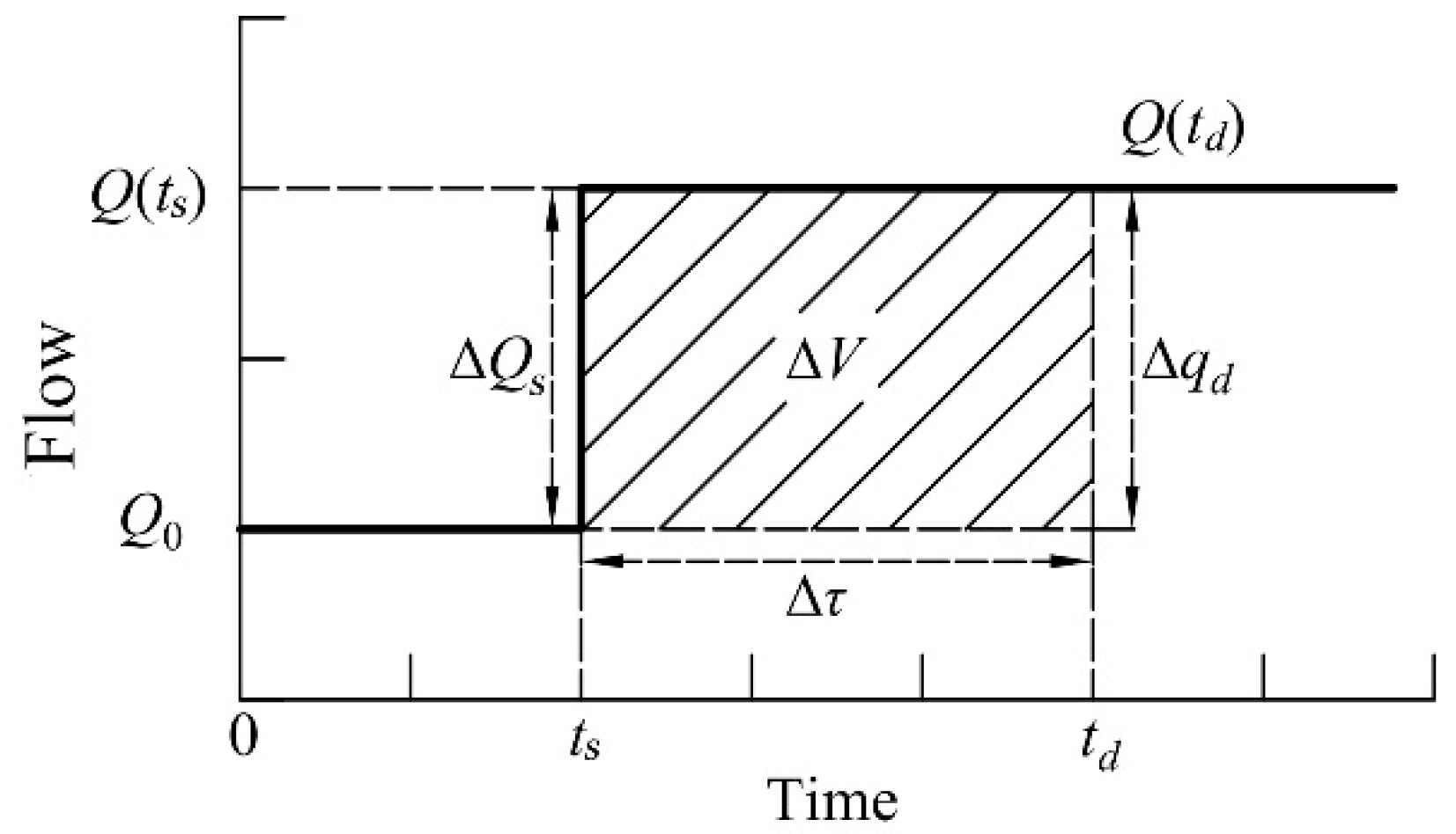
The calculation of canal pool’s storage is related to the geometric parameters, roughness, upstream and downstream boundary conditions of the canal pool, water intake plans and so on [5]. On this basis, the volume step compensation algorithm assumes that a series of intermediate stable states in the operation process exist. As shown in Figure 1, in the case of a single canal pool, according to the water intake plan, the flow should be changed by Δqd at td. From the assumed initial state, it can be deduced that the storage of the canal pool needs to be adjusted by ΔV, i.e., the initial flow Q0 is adjusted Q0 +ΔQs at ts. At td, the storage of the canal pool can be adjusted completely. The meaning of the volume step compensation is to adjust the discharge of the canal pool once in advance. When the intake begins to take water, the adjusted storage can satisfy the storage required by the current intake of the canal pool, and the flow need not be adjusted again. At this time, ΔQs is equal to Δqd. The delay time Δτ is the difference between ts and td. Its calculation is shown in Equation (1).
2.2. Dynamic Wave Principle Algorithm
The delay time of the volume step compensation algorithm is deduced according to the storage and flow required by currrent water demand of the canal pool. Even for a given canal pool, the delay time will vary with the different intake water. In the process of channel operation, when the downstream water demand plan is determined, the value of volume compensation is determined, but its realization is not the only way. For example, the storage compensation can be carried out with small flow change and a long delay time, and vice versa, with a large flow change and shorter delay time. The phenomenon of water wave lag is mainly related to the movement of water wave in the canal pool. Corriga [9] calculates the delay time by using the water wave characteristics of the initial state, as shown in Equation (2). Because the average velocity and wave velocity of the initial state are adopted without considering the attenuation of energy in the process of water wave propagation, the delay time calculated by the algorithm is the smallest [5] in the methods mentioned in this paper.
In Equation (2), ΔτDW is the delay time of dynamic wave principle calculation; L is the length of canal pool, (m); v0 is the initial average velocity of canal, (m/s); c0 is the initial average velocity, (m/s).
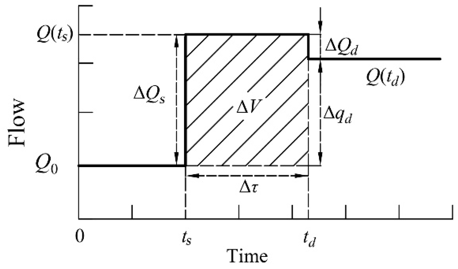
In the dynamic wave principle algorithm, the flow regulation can be deduced according to the ideal delay time [9] on the basis of known storage variation. In fact, the flow regulation is not equal to the target value, so there is secondary regulation, i.e., to adjust the flow to the target value after reaching the target time. As shown in Figure 2, the initial discharge Q0 of the canal pool is adjusted to Q(ts) at ts, and from ΔQd to the target value Q(td) at td. The purpose of secondary regulation is to avoid the waste of water when the intake opens and the inflow of the canal pool exceeds the flow required by the intake.
2.3. Water Balance Model Algorithm
When the downstream users have water requirements, the upstream canal pools will transport the corresponding water to the downstream and be used by the downstream users to complete the whole water distribution process. In the channel operation, downstream water intake produces upstream precipitation wave and upstream water supply produces upstream water wave, which is superimposed by non-linear superposition. It is difficult to determine feedforward control time when unsteady flow is used for calculation. In order to calculate the delay time, the analytical formula of downstream canal pool response is introduced into the algorithm, as shown in Equation (3) [13].
In the formula, q(x,t) is the flow at canal pool x at t, (m3/s); τ(x) is the delay time at canal pool x, (s); K(x) is the time parameter at canal pool x, (s). In order to determine the time of water intake, the process of water intake and supply is simplified to a linear equation and superimposed [10], as shown in Equations (4)–(6).
When t τ,
When τ < t < Tw,
When t Tw,
where K is the time constant introduced in the process of water wave propagation; Kp is the time parameter introduced by the change of downstream intake flow; qd(t) is the change of downstream flow at t time, (m3/s); δQu is the upstream water supply, (m3/s); kd is the flow coefficient, indicating the sensitivity of time parameter K to the influence of downstream flow and water level boundary, (m2/s); qw,0 is the downstream intake flow, (m3/s); Tw is the optimal intake time; a is the sudden drop of water level caused by intake, (s/m2), τ is the delay time of parameter identification of water balance model. In order to minimize the downstream discarded water, the upstream water supply quantity δQu is equal to the downstream water intake quantity qw,0. At this time, the canal pool does not produce discarded water, and the calculation formula of the optimal water intake time is demonstrated in Equations (7) and (8). In Equation (7), tw is the difference between the optimal water intake time and the delay time of the canal pool. In the actual simulation process, K, τ, Kp, a and kd parameters can be obtained by the parameter identification method.
3. Delay Time Explicit Algorithm
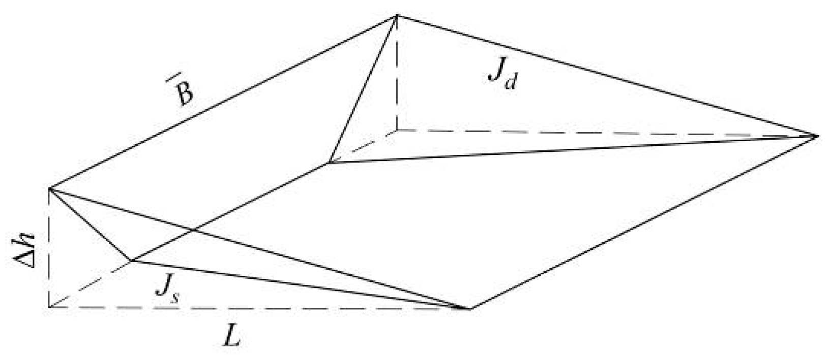
According to the volume step compensation algorithm, the storage capacity of the canal pool is calculated mainly by the relationship between the water surface of the constant and non-uniform flow, which requires numerical discrete calculation. In order to avoid the discrete calculation needed for deducing storage, this section seeks to find a formula that can directly calculate delay time according to canal pool geometry size and flow state, namely delay time explicit algorithm. In general, the compensatory storage of canal pool is affected by the flow variation of water demand. According to Equation (1), when the flow variation of water demand in canal pool is determined, the delay time Δτ of the canal pool is proportional to the compensation value ΔV of water demand in canal pool. In this paper, the open channel constant gradient flow theory [14] is used for analysis. When the canal pool is running at the downstream constant water level, the volume of storage change in the canal pool can be approximately considered as a wedge-shaped water body rotating around the control point (Figure 3). For the artificial trapezoidal section canal pool, the hydraulic gradient J of the open channel steady gradient flow can be calculated by Equation (9).
In Equation (9), Q is the discharge of the canal pool, (m3/s); K′ is the flow modulus, (m3/s); v is the average velocity of the canal, (m/s); C is the Chezy coefficient; R is the hydraulic radius, (m); n is the roughness; A is the area of the control point, (m2). When the bottom slope of the canal pool is gentle and the water demand changes a little, the difference of A, R and B upstream before and after the volume compensation of the canal pool is small and the average values of the two points are calculated.
The actual process of solving J is often complex. To simplify the solution, J is expanded into Taylor polynomial near a certain flow to approximate it. When the bottom slope of the canal pool is gentle and the change of water demand is small, the difference of J under different discharge is small, so Taylor polynomial only expands to the second term in Equation (10). ΔJ is the second item of hydraulic gradient developed by the Taylor polynomial, i.e., the difference between the hydraulic gradient Jd and Js before and after the volume compensation. The estimation of the required compensation value ΔV of the canal pool is shown in Equations (11)–(13).
In Equation (13), is the average flow area upstream of the canal pool before and after the volume compensation, m2; is the average water surface width upstream of the canal pool before and after the volume compensation, m; is the average hydraulic radius upstream of the canal pool before and after volume compensation, m. According to Equation (1), the relationship between the delay time Δτ and the flow of the change of water demand Δqd can be attained. However, in practical engineering, due to the influence of length L, initial discharge Q0 and different water demand variation, the delay time calculated by , , is smaller than actual delay time. That is to say, there exists amplification coefficient αam to correct the calculation results. In Equation (13), when the initial and final discharge of the canal pool is determined, the main factors affecting the required volume are the geometric parameters of the canal pool, including the length, width of the canal bottom and so on. Combining with the geometric parameters of the canal pool, this paper introduce an empirical formula of αam on the length and width of the canal bottom to correct the delay time (Equation (14)). The relationship between the delay time Δτ and the flow Δqd of the change of water demand is shown in Equation (15). The coefficients a and c are calculated in Equation (16).
4. Simulation Settings
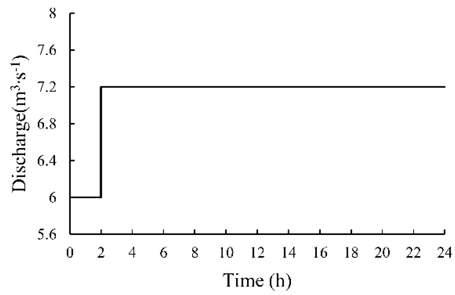
Considering that the delay time of multi-channel pools in series is affected by the coupling effect of canal pools [15], i.e., the function of a single gate will cause the change of water level and discharge of several canal pools upstream and downstream, and the action of each gate will influence each other, this simulation model of single canal pool is built, i.e., canal pool 1 in ASCE Test Canal 2 [12]. The length of the canal pool is 7 km, the bottom slope is 0.0001, the roughness is 0.02, the slope is 1.5, the width of the canal bottom is 7 m, and the intake is located the most downstream of the canal pool. The total simulation time is 24 hours and the time step is 3 min. The downstream flow of the canal pool remains unchanged at 6 m3/s. As shown in Figure 4, in the second hour, the intake begins to take 1.2 m3/s, and the upstream flow of the canal pool changes from 6 m3/s to 7.2 m3/s (Figure 4).
The parameters identified by the water balance model algorithm [10] are shown in Table 1 [16]. The delay time calculated by four algorithms is shown in Table 2. Theoretically, the optimal intake time obtained by the water balance model algorithm should be equal to the delay time obtained by the volume step compensation algorithm, and the former algorithm needs to identify five parameters which are shown in Table 1. The delay, time calculated by the volume step compensation algorithm, needs to estimate the required volume by assuming a constant non-uniform flow line relationship between the initial and the final. It needs to discretize the canal pool in order to resolve the water surface line. The accuracy of parameter identification and the error of water surface line calculation will affect the results of the two algorithms. In the example, the delay time calculated by volume step compensation algorithm is 12.46 min less than the optimal intake time deduced by water balance model algorithm. According to the geometric parameters of the canal pool, the length and bottom width are substituted into Equation (14), and the amplification factor αam of the canal pool is 1.75.
5. Results and Discussion
In order to compare the control effects of different algorithms, four performance indicators, i.e., transition time, maximum overshot flow, integral of absolute magnitude of error (IAE) and integrated absolute discharge change (IAQ) are selected. IAQ characterizes the fluctuation of the flow in the canal pool. The smaller the value, the more stable the system is, i.e., the smaller the flow fluctuation in the canal pool. IAE is the error accumulation of the water level deviating from the target water level. The smaller the value, the smaller the error range of the water level is. At this time, the smaller the gate actions of the channel control system are needed, and the faster the canal pool can reach the steady state [12]. The control performance indicators of the four algorithms are shown in Table 3. From the relationship of indicators, IAQ describes the flow fluctuation process in the regulation process of canal pool, and the range of flow fluctuation is affected by the maximum overshot flow. If the value of the maximum overshot flow is large, in order to make the flow of canal pool adjust to the steady flow state, the more regulations are needed, which causes the large the IAQ value. In Table 3, the maximum overshot flow of volume step compensation, water balance model and delay time explicit algorithm is close to the target flow of 7.2 m3/s, and the IAQ value is small. However, the dynamic wave principle algorithm uses ideal delay time to compensate the storage by increasing the inflow of the canal pool. At this time, the maximum overshot flow exceeds the target flow by 0.644 m3/s, which is reflected in the IAQ value. The IAQ value of the dynamic wave algorithm is about 43.67 times that of the volume step compensation algorithm, and the flow regulation fluctuates significantly.
The simulation process of the canal pool discharge is shown in Figure 5. The volume step compensation and the delay time explicit algorithm can basically achieve the target flow in the canal pool by adjusting the flow only once. However, the dynamic wave principle uses the initial flow velocity and wave velocity of the canal pool to estimate the delay time, and the obtained delay time is small. In order to meet the demand of the current required storage volume, the flow of the canal pool is over-adjusted to 7.844m3/s for compensation of the storage. After the water intake is opened, in order to avoid the waste of water, the flow of the canal pool is adjusted to the target flow for the second time. According to the compensated storage volume and the optimal intake time of the canal pool, the water balance model can calculate the flow value of the canal pool adjusted in advance. Affected by parameter identification, the optimal intake time of the calculation is slightly large. In order to meet the demand of the canal pool storage, the canal pool can adopt a small flow to compensate the storage capacity, i.e., the flow of the canal pool adjusted in advance is 6.843 m3/s, which is less than the target flow (7.2 m3/s). Then the flow of the canal pool increases to the target state, so as to avoid the phenomenon of insufficient water supply after opening the intake.
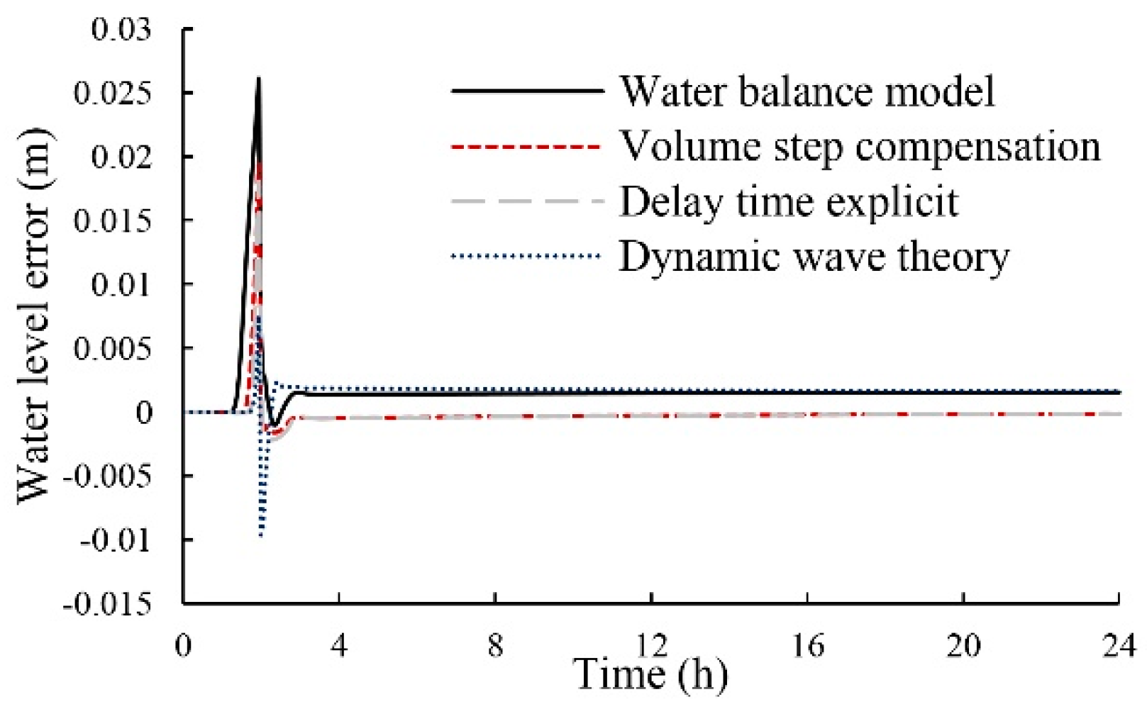
The fluctuation of flow also affects the fluctuation of water level. The water level errors of downstream control points of the four algorithms are shown in Figure 6. Feedforward controllers are regulated according to plan and lacks real-time feedback mechanism. That is to say, the water level error of downstream control point of canal pool cannot converge to zero completely after adjustment, and the water level error will remain in a stable range. Taking the convergence of the water level error to zero as a reference, feedforward control algorithms compensate the storage of the canal pool by increasing the inflow ahead of time, and the water level at the downstream control point is higher than the target water level (the water level error is greater than 0). When the water intake begins, the water level at the downstream control point of the canal pool gradually falls and fluctuates. After stabilization, the water level error at the downstream control point remains within a stable range. Different feedforward control algorithms have different adjustment effects. After being adjusted by the volume step compensation or delay time explicit algorithm, the water level error of the downstream control point is stable at −0.0001 m, which is close to 0 basically. After being adjusted by the dynamic wave principle algorithm or water balance model, the water level error of downstream control point is stable at 0.002 m. IAE describes the accumulation of water level errors in the regulation process. In Table 3, the IAE of the water balance model algorithm is also the largest, and the IAE of the dynamic wave principle algorithm is slightly smaller than that of the water balance model algorithm, indicating that the errors accumulation of the water level deviating from the target water level is also greater. The IAE of the volume step compensation and the delay time explicit algorithm is smaller than the other two algorithms. The transition time of different control algorithms is affected by the fluctuation of flow and water level in the canal pool. When the IAQ and IAE of the canal pool are small, the time spent to reach the stable state of the canal pool is also less. In Table 3, the volume step compensation algorithm’s IAE and IAQ are small, and the transition time is the shortest. The flow fluctuation of canal pool is large during the adjustment process of dynamic wave principle algorithm, which results in the longest transition time. When the fluctuation of flow in the canal pool is small (IAQ is small), the transition time is mainly affected by the water level fluctuation of canal pool. The IAE of the water balance model algorithm is slightly larger than that of the delay time explicit algorithm, so the transition time of the algorithm is slightly longer than that of the delay time explicit algorithm.
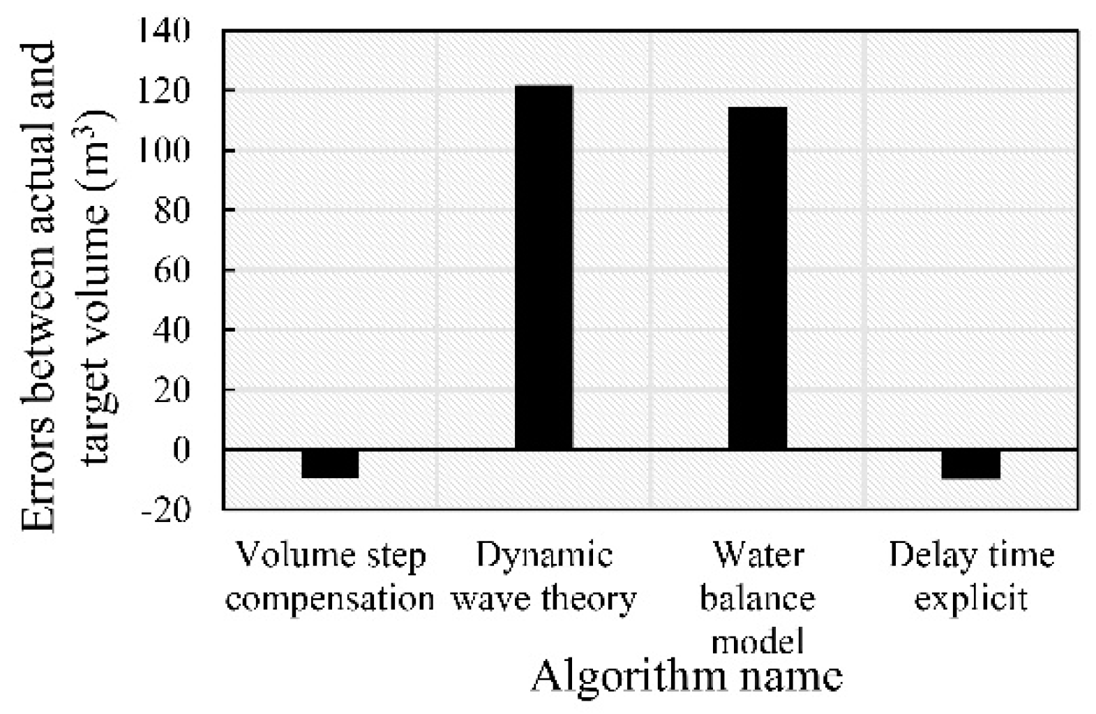
Feedforward control algorithms rely on water intake plan to adjust the input of control system in advance. If the amount of adjustment is too large in advance, it will cause unnecessary waste of water resources. The target compensation storage of the canal pool is 2628.4 m3. The difference between the actual storage and the target storage of four algorithms are shown in Figure 7. Compared with the volume step compensation algorithm and delay time explicit algorithm, the actual compensation storage of the other two algorithms exceeds the target storage. The actual storage of the dynamic wave algorithm after water intake exceeds the target storage 121.79 m3, the actual storage of the water balance model algorithm after water intake exceeds the target storage 114.64 m3. In order to maintain the stability of the control system, the excess storage should be drained from the downstream. The dynamic wave principle algorithm is based on the velocity and velocity of the flow in the initial state of the canal pool, without considering the energy attenuation in the process of water flow propagation. The delay time calculated by this algorithm is small. In order to fully compensate the storage required by the canal pool, the flow of the storage compensation will be larger than the target flow. When the water intake is started, the flow of the canal pool will be adjusted to be equal to the target flow, so as to avoid the inflow of the canal pool being larger than the flow required by the canal pool, resulting in the waste of water resources. However, in the process of regulating the canal pool, the discharge has been adjusted twice, which results in the fluctuation of the water level and discharge of the canal pool, and the operation needed to stabilize the canal pool is more, which leads to a greater waste of water. Based on the principle of water balance in the canal pool, the water balance algorithm assumes that the canal pool does not produce discarded water, and derives the equation for calculating the optimal intake time. In practice, the optimal water intake time is obtained by identifying the K, τ, Kp, a and kd parameters of the canal pool under water intake and supply processes. The identification accuracy of the five parameters will affect the optimal intake time. In the current example, the optimal intake time obtained is slightly large, and the actual adjusted storage exceeds the target.
While the actual storage of the volume step compensation algorithm is 9.68 m3 less than the target storage, and the actual storage of the delay time explicit algorithm is 9.82 m3 less than the target storage. The volume step compensation algorithm calculates the delay time by assuming the steady state at the beginning and the end. In order to calculate the storage of the canal pool, it is necessary to discretize the canal pool in space and obtain the water surface profile of the constant non-uniform flow. In order to ensure the continuity of the calculation of the water surface line, the water surface line will be smoothed at discrete points. At the same time, the algorithm ignores the intermediate state of the actual adjustment, so the actual storage adjustment value of the algorithm is slightly smaller than the target storage. The delay time explicit algorithm assumes that the change of the A, B and R of the canal pool before and after intake is small. Therefore, the delay time obtained by using the average value , , is smaller than actual delay time and needs to be corrected by amplification coefficient. However, only considering the influence of the canal pool length and bottom width, this paper calculates the amplification factor by using a simple empirical formula (Equation (14)). The actual compensation storage is slightly smaller than the target storage. In practice, the measured data (flow or water level) and more geometric parameters of the canal pool should be taken into account to correct this empirical formula. The percentage of the actual compensation storage of the four algorithms to the target compensation storage is shown in Table 4.
6. Conclusions
Under the operation mode of downstream constant water level of Canal Pool 1 in ASCE Test Canal 2, combining the theory of open channel constant gradient flow with volume compensation, this paper introduces a delay time explicit algorithm, and discusses the operation control effect of three existing algorithms of volume step compensation, dynamic wave principle, water balance model and delay time explicit algorithm. The conclusions are as follows:
(1) The delay time explicit algorithm establishes a linear formula between the delay time and the flow change required by water demand, which avoid the space discrete calculation of canal pool needed for storage estimation or identification of relevant parameters. Under the current water intake plan, only 1.47 h is needed to achieve stability of the canal pool. During the regulation process, the fluctuation of water level and flow in the canal pool is small. The actual adjusted storage accounts for 99.6% of the target adjusted storage, which basically meets the requirement of compensated storage required by the canal pool. The delay time calculated by the explicit algorithm can provide some references for the determination of delay time in feedforward control.
(2) Among the three existing algorithms, the volume step compensation algorithm has better control effect. Under the current water intake plan, the volume step compensation algorithm needs 1.25 hours to achieve stability, and the water balance model algorithm needs 1.77 hours to achieve stability. While the dynamic wave principle algorithm has secondary flow adjustment, the transition time is the longest among the three methods, and the flow fluctuates during the regulation process. The actual adjusted storage of volume step compensation algorithm accounts for 99.6% of the target adjusted storage, which basically meets the requirement of compensated storage for the canal pool. While the actual adjusted storage of the other two algorithms exceeds the target storage, which means the generation of discarded water.
However, in order to avoid the coupling effect of series canal pools, the case of single canal pools is only considered in this paper, and the case of multi-channel pools in series requires further discussion. At the same time, the paper only considers the influence of canal pool length and bottom width, and further calculates the amplification coefficient by using the simple empirical formula in the delay time explicit algorithm. In the actual process, the measured data (flow or water level) and the other geometric parameters of the canal pool should be taken into account to correct the empirical formula.
Author Contributions
All authors have contributed substantially to this work, as specified below: writing—original draft preparation, W.L.; writing—review and editing, G.G. and X.T.
Funding
This research was funded by National Key R&D Program of China (Grant No. 2016YFC0401810) and National Natural Science Foundation of China (No. 51439006).
Acknowledgments
The authors appreciate the comments from the anonymous reviewers.
Conflicts of Interest
The authors declare no conflict of interest.
References
- Ni, W.J. Development and technology requirement of China rural water conservancy. Trans. Chin. Soc. Agric. Eng. 2010, 26, 1–8. [Google Scholar] [CrossRef]
- Wang, H.; Wang, J.H. Sustainable utilization of China’s water resources. Bull. Chin. Acad. Sci. 2012, 27, 352–358. [Google Scholar] [CrossRef]
- Wylie, E.B. Control of transient free-surface flow. J. Hydraul. Div. 1969, 95, 347–362. [Google Scholar]
- Cunge, J.A.; Holly, F.M.; Verwey, A. Practical Aspects of Computational River Hydraulics; Pitman Advanced Publishing Program: Boston, UK, 1980; ISBN 0273084429. [Google Scholar]
- Bautista, E.; Clemmens, A. Volume compensation method for routing irrigation canal demand changes. J. Irrig. Drain Eng. 2005, 131, 494–503. [Google Scholar] [CrossRef]
- Cui, W.; Chen, W.; Guo, X. Anticipation time estimation for feedforward control of canal. In Proceedings of the 33rd IAHR Congress, Vancouver, BC, Canada, 9–14 August 2009; pp. 1529–1536. [Google Scholar]
- Soler, J.; Gomez, M.; Rodellar, J. GoRoSo: Feedforward Control Algorithm for Irrigation Canals Based on Sequential Quadratic Programming. J. Irrig. Drain Eng. 2013, 139, 41–54. [Google Scholar] [CrossRef]
- Burt, C.M.; Feist, K.E.; Xianshu, P. Accelerated Irrigation Canal Flow Change Routing. J. Irrig. Drain Eng. 2018, 144, 1–9. [Google Scholar] [CrossRef]
- Corriga, G.; Fanni, A.; Sanna, S.; Usai, G. A constant-volume control method for open channel operation. Int. J. Simul. Model. 1982, 2, 108–112. [Google Scholar] [CrossRef]
- Belaud, G.; Litrico, X.; Clemmens, A.J. Response time of a canal pool for scheduled water delivery. J. Irrig. Drain Eng. 2013, 139, 300–308. [Google Scholar] [CrossRef]
- Simulation and Control of Canal System. Available online: http://www.ccopyright.com.cn/ (accessed on 3 June 2011).
- Clemmens, A.J.; Kacerek, T.F.; Grawitz, B.; Schuurmans, W. Test cases for canal control algorithms. J. Irrig. Drain Eng. 1998, 124, 23–30. [Google Scholar] [CrossRef]
- Munier, S.; Litrico, X.; Belaud GMalaterre, P. Distributed approximation of open-channel flow routing accounting for backwater effects. Adv. Water Resour. 2008, 31, 1590–1602. [Google Scholar] [CrossRef] [Green Version]
- Te Chow, V. Open-Channel Hydraulics; The Blackburn Press: West Caldwell, UK, 2009; ISBN 1932846182. [Google Scholar]
- Cui, W.; Chen, W.; Mu, X.; Bai, Y. Canal controller for the largest water transfer project in China. Irrig. Drain 2015, 63, 501–511. [Google Scholar] [CrossRef]
- Huang, K. Simulation for Time Model of Feedforward Control and Modified PID Feedbackalgorithm on Tandem Canal System. Master’s Thesis, Wuhan University, Wuhan, China, 2016. [Google Scholar]
Figure 1.
Schematic diagram of volume step compensation algorithm.

Figure 2.
Schematic diagram of volume compensation algorithm with two adjustments.

Figure 3.
Schematic diagram of wedge-shaped water body.

Figure 4.
Change process of canal pool discharge according to intake plan.

Figure 5.
Simulation process of canal pool discharge.

Figure 6.
Water level error of downstream control point.

Figure 7.
Differences between actual and target storage of canal pool after water intake.


Table 1.
Parameters identified by water balance model algorithm.
| K/min | τ/min | Kp/min | a/(s∙m−2) | kd/(m2∙s−1) | Tw/min |
|---|---|---|---|---|---|
| 67.6 | 29 | 63.8 | 0.026 | 15.9 | 51.46 |
Table 2.
Delay time calculated by four algorithms.
| Algorithm Name | Volume Step Compensation | Dynamic Wave Principle | Water Balance Model | Delay Time Explicit |
|---|---|---|---|---|
| Delay time/min | 39 | 24 | 51.46 | 37 |
Table 3.
Performance indicators of canal pool.
| Algorithm Name | Transition Time/h | Maximum Overshot Flow/(m3∙s−1) | IAE/% | IAQ/(m3∙s−1) |
|---|---|---|---|---|
| Volume step compensation | 1.25 | 7.201 | 3.65 × 10⁻⁶ | 0.030 |
| Dynamic wave principle | 2.55 | 7.844 | 1.49 × 10⁻⁵ | 1.313 |
| Water balance model | 1.77 | 7.201 | 1.53 × 10⁻⁵ | 0.033 |
| Delay time explicit | 1.47 | 7.201 | 3.62 × 10⁻⁶ | 0.097 |
Table 4.
Percentage of actual compensation storage to target compensation storage.
| Algorithm Name | Volume Step Compensation | Dynamic Wave Principle | Water Balance Model | Delay Time Explicit |
|---|---|---|---|---|
| Percentage/% | 99.6 | 104.6 | 104.4 | 99.6 |
© 2019 by the authors. Licensee MDPI, Basel, Switzerland. This article is an open access article distributed under the terms and conditions of the Creative Commons Attribution (CC BY) license (http://creativecommons.org/licenses/by/4.0/).
Share and Cite
MDPI and ACS Style
Liao, W.; Guan, G.; Tian, X. Exploring Explicit Delay Time for Volume Compensation in Feedforward Control of Canal Systems. Water 2019, 11, 1080. https://doi.org/10.3390/w11051080
AMA Style
Liao W, Guan G, Tian X. Exploring Explicit Delay Time for Volume Compensation in Feedforward Control of Canal Systems. Water. 2019; 11(5):1080. https://doi.org/10.3390/w11051080
Chicago/Turabian StyleLiao, Wenjun, Guanghua Guan, and Xin Tian. 2019. "Exploring Explicit Delay Time for Volume Compensation in Feedforward Control of Canal Systems" Water 11, no. 5: 1080. https://doi.org/10.3390/w11051080
Note that from the first issue of 2016, this journal uses article numbers instead of page numbers. See further details here.