Water Pump Control: A Hybrid Data-Driven and Model-Assisted Active Disturbance Rejection Approach

Abstract

Water pump control, prevalent in various industrial plants, such as wastewater treatment and steam generator facilities, plays a significant role in maintaining economic efficiency and stable plant operation. Due to its slow dynamics, strong nonlinearity, and various disturbances, it is also widely studied as a typical benchmark problem in process control. The current control strategies can be categorized into two aspects: one branch resorts to model-based design and the other to data-driven design. To merge the merits and overcome the deficiencies of each paradigm, this paper proposes a hybrid data-driven and model-assisted control strategy, namely modified active disturbance rejection control (MADRC). The model information regarding water dynamics is incorporated into an extended state observer (ESO), which is used to estimate and mitigate the limitations of slow dynamics, strong nonlinearity, and various disturbances by analyzing the real-time data. The tuning formula is given in terms of the desired closed-loop performance. It is shown that MADRC is able to produce a satisfactory control performance while maintaining a low sensitivity to the measurement noise under general parametric setting conditions. The simulation results verify the clear superiority of MADRC over the proportional-integral (PI) controller and the conventional ADRC, and the results also evidence its noise reduction effects. The experimental results agree well with the simulation results based on a water tank setup. The proposed MADRC approach is able to improve the control performance while reducing the actuator fluctuation. The results presented in this paper offer a promising methodology for the water control loops widely used in the water industry.

1. Introduction

Water pump control, which is widely used in various chemical industries [1,2,3], such as in regenerative heaters [4] and drum boilers [5], petrochemical processes [6], open channels [7], surge tanks of hydropower stations [8], and steam generators [9,10,11,12], plays a significant role in maintaining economic efficiency and stable plant operation. For instance, in thermal power plants, the drum boiler water level is a key parameter in monitoring boiler operational conditions, which indirectly reflects the balance between the steam load and water supply. An appropriate pump control design is able to maintain the water level and thus guarantee the safe operation of the boiler [13]. Furthermore, for nuclear steam supply systems, one of the most important control strategies of such a system is steam generator water level regulation to preserve the level around programmed setpoint, because the reduction of the water level jeopardizes the heat removal from the reactor, and increasing the level will cause the humidity of the generated steam to rise, causing severe erosion of the turbine blades [11].

However, water control is challenging due to slow dynamics, strong nonlinearity, and various disturbances. There are many proposed control strategies in the literature to design water level control systems (see e.g., [14,15,16]). Among the most widely used techniques are simple fixed gain proportional-integral (PI) controllers. A model-free control has also been proposed to address the multivariable nonlinear finite-dimension and important unknown disturbances and to ensure that the water level reaches the setpoint [7]. Additionally, a new global water level control of horizontal steam generator was designed using the quantitative feedback theory [9]. A gain scheduled fractional-order proportional-integral-derivative (PID) control system has also been used to control steam generator levels over an entire operating range [11]. Moreover, an adaptive estimator-based dynamic sliding mode control method was developed to address the level control problem [10].

It is regrettable that none of the above controllers combine model information with real-time input and output data, such that disturbances affecting these models cannot be compensated by real-time data. In addition, it is well known that noise has a negative impact on the executing agencies in industrial processes, but the noise generated by fluctuations in water level has not drawn much attention in the above literature. Therefore, this paper introduces a new controller with the above two problems taken into account. The proposed controller can compensate for disturbances in real time so as to control the water level accurately and suppress the influence of noise in the system.

The current process control strategies can be categorized in two aspects. One branch utilizes model-based control design, in which much effort is put into developing a class of accurate models under different operation conditions. Then, the controller is designed by taking into consideration the detailed dynamics, nonlinearity, and uncertainty information. To overcome the robustness deficiency of the model-based design, the other branch chooses to avoid the tough modeling work and adopts a data-driven method, such as active disturbance rejection control (ADRC) [17]. Under this data-driven paradigm, the unknown dynamics, nonlinearity, and uncertainty are treated as a lumped disturbance term that can be estimated and mitigated by analyzing real-time data. A combination of two data-driven techniques—the virtual reference feedback tuning and model-free control—was proposed to serve as a control system [18]. A novel multi-agent-based data-driven distributed adaptive cooperative control method was also investigated for multi-direction queuing strength balance with changeable cycles in urban traffic signal timing [19]. Two new control structures referred to as second-order, data-driven active disturbance rejection control combined with proportional-derivative Takagi-Sugeno fuzzy control are proposed, which consists of a second-order, data-driven active disturbance rejection control and a proportional-derivative Takagi-Sugeno fuzzy logic controller [20].

Although robust, this new method may suffer from strong sensitivity to the measurement noise, which is harmful for the actuator. Relatively large inertia and strong measurement noise are often encountered in industrial water pump control processes that challenge the precision and stability of industrial water pump control, especially in terms of the following aspects:

• For a large inertia of the system, it is difficult for the conventional proportional–integral–derivative (PID) controller to achieve good control performance. Specifically, for the reference tracking control, the conventional PID control suffers from integral saturation, which leads to large overshoot and even sustained oscillation.
• The measurement noise will directly influence the output control variable in the closed-loop control. In particular, the high-frequency noise caused by the low resolution of the measurement device in the industrial process will cause large fluctuation to the control variables, which may cause irreversible damage and shorten the life span of the actuator under serious conditions.

In order to solve the second problem mentioned above, a low-pass filter is usually added at the output terminal to reduce the fluctuation of output control variables and protect the actuators. However, it is well known that the introduction this filter will attenuate the control variables and thus weaken the controller performance.

Simple yet effective, the PID controller has flourished in industry in recent years [21]. However, the ever-increasing demands on accuracy, robustness, and efficiency, coupled with the inherent limitations of the PID, have driven engineers to seek better control methods elsewhere. In recent years, the ADRC as a promising new control design framework has emerged as a viable alternative. It offers a timely, if not conventional, solution to practical problems [22]. The essence of the ADRC is an effective control strategy for dealing with unknown disturbances and uncertainties. Its robustness property to changes in dynamics and external disturbances has been repeatedly demonstrated in practical applications [23,24].

In the ADRC application, the influence of the model uncertainty and the external unknown disturbances is observed by the extended state observer (ESO) based on the input-output data of the system. The control is then given to compensate for these disturbances, thereby greatly reducing the effect of the disturbance. From the frequency domain point of view, such a control method is far ahead of the general “error-based” controller in terms of phase, namely, the control function is ahead of the ordinary PID control, thereby having a better control effect.

The flourishing achievements in both academia and industry applications of the ADRC, for instance, in motion control [25,26] and process control [27,28], can be attributed to its simple structure, ease of tuning, and excellent control performance [29].

A combined structure of the feedforward and the ADRC is proposed in [30] to address the difficulties in controlling the non-minimum phase (NMP) systems. Inspired by this, along with the characteristics of practical controlled systems, the information on the system model is added to the ESO, resulting in an improved ESO for the ADRC. Compared with the conventional ADRC, the modified ADRC (MADRC) proposed in this paper features as the following itemized points:

• The estimation accuracy is improved by incorporating the model information;
• The control performance is improved in terms of both set-point tracking and disturbance rejection;
• The control action is experimentally demonstrated to be less sensitive to the measurement noise.

In this paper, on the basis of theoretical deduction, we will verify two remarkable performances of the proposed MADRC compared with ADRC and PID through experiments: (1) excellent set-point tracking ability and (2) noise suppression ability. It is worth noting that in this paper, we first deduce a theoretical noise reduction condition for the controller and then verify it in simulation experiments and practical experiments. The remainder of the paper is organized as follows: Section 2 presents the structure of the modified ESO and the MADRC. The noise problem in the close-loop is formulated in Section 3, and the noise suppression ability of the MADRC is analyzed. The controller design and simulation experiment are given in Section 4. A comparative study is carried out by hardware experiment in Section 5, and the conclusions are reached in Section 6.

2. Structure of Modified ADRC

In this section, we will gradually introduce the structure of MADRC in theory. For the sake of universality and verifiability, the controller structure and noise reduction conditions mentioned in this paper are not specific to any system or object.

2.1. Fundamentals of ADRC

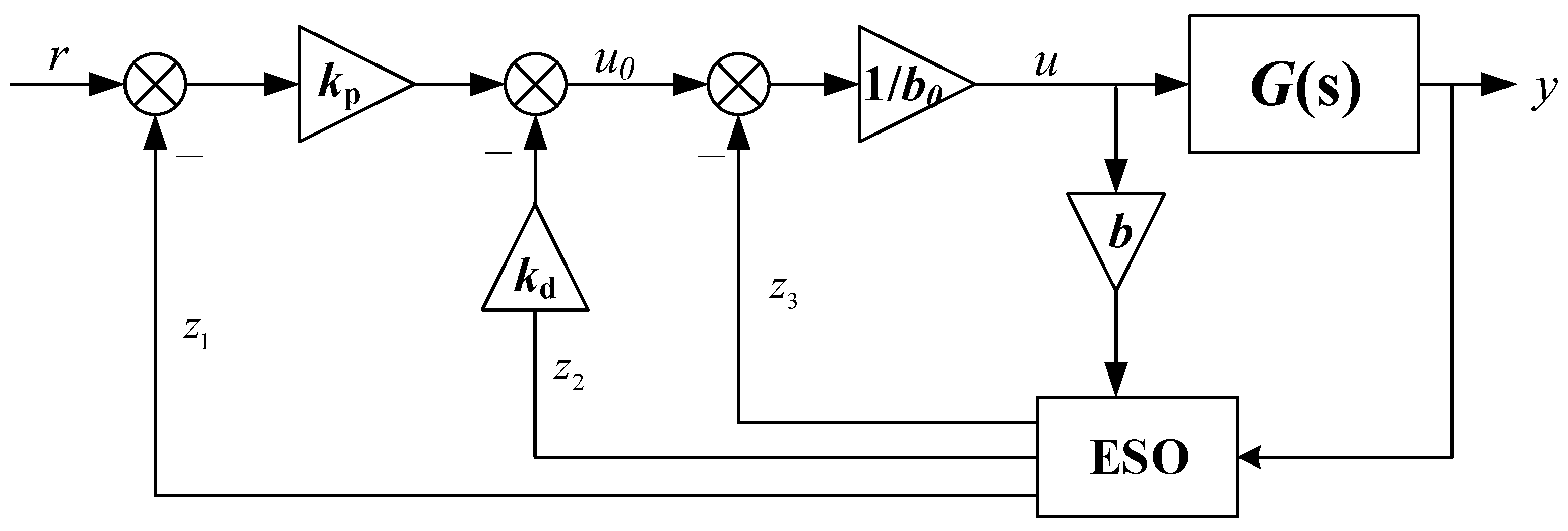
Recognizing the fact that most of the industrial processes are represented by second-order systems, the objective of this paper is also to design controllers for second-order systems. The structure of the second-order ADRC is shown in Figure 1, where r is the reference input; y denotes the system output; u₀ is the control variable of controller; s is the Laplacian operator; k_p, k_d, and b₀ are the controller parameters; b is a gain parameter; G(s) represents controlled object; u is control variable for G(s); and z₁, z₂, and z₃ are the estimation of system state variables.

Consider G(s) as a second-order system with single-input u and single-output y,

$$\ddot{y}(t)=f\left(y(t),\dot{y}(t),w(t)\right)+bu(t)$$

(1)

where w is the external disturbance, b is a gain parameter, and f denotes an unknown combination of the system states and disturbances. By extending the ‘total disturbance’ f as an additional state, the system (1) can be represented as an augmented state-space model.

$$\begin{array}{l}\dot{x}=Ax+Bu+Eh\\ y=c^{T}x\end{array}$$

(2)

where $x={\left[x_1,x_2,x_3\right]}^T={\left[y,\dot{y},f\right]}^T, h=\dot{f}, c^T=\left[100\right]$, T denotes transposition and

$$A=\left[\begin{array}{lll}0& 1& 0\\ 0& 0& 1\\ 0& 0& 0\end{array}\right],B=\left[\begin{array}{l}0\\ b\\ 0\end{array}\right],E=\left[\begin{array}{l}0\\ 0\\ 1\end{array}\right]$$

(3)

An extended state observer (ESO) is designed for system (2) accordingly as follows:

$$\begin{array}{l}\dot{z}=Az+Bu+\beta (y-z_1)\\ \widehat{y}=c^{T}z\end{array}$$

(4)

where, z = [z₁, z₂, z₃]^T aims at tracking x, and β = [β₁, β₂, β₃]^T is the observer gain. The observability and controllability of the extended plant (3) as well as the convergence of ESO (4) are analyzed in [30].

For simplicity of tuning, referring to the bandwidth parameterization method [31], the observer gain can be obtained by setting the characteristic equation of (4) as ϕ(s) = (s + ω_o)³, where ω_o is the desired observer bandwidth. Accordingly, the characteristic equation of (4) is

$$\varphi (s)=s^3+{\beta }_1{s}^2+{\beta }_{2}s+{\beta }_3={\left(s+{\omega }_o\right)}^3$$

(5)

from which the observer gain is calculated as

$$\{\begin{array}{l}{\beta }_1=3{\omega }_o\\ {\beta }_2=3{\omega }_o^2\\ {\beta }_3={\omega }_o^3\end{array}$$

(6)

The convergence of ESO was proved in [32]. By compensating the estimated total disturbance z₃ in real time as

$$u=\frac{u_0-z_3}{b}$$

(7)

the original system (1) can be reduced to

$$\ddot{y}=f+bu=f+u_0-z_3\approx u_0$$

(8)

which is the enforced plant with the disturbance estimate, approximated as cascaded integrators. Then, the controller for the enforced plant (8) can be determined simply as a state feedback law, as follows:

$$u_0=k_{\mathrm{p}}\left(r-z_1\right)-k_{\mathrm{d}}{z}_2$$

(9)

where r is the reference output. The tracking error of the control law is proved to be bounded in [32], provided that the derivative of f is bounded. The observer gain β and feedback gain k_p and k_d can be easily tuned based on the bandwidth parameterization method in [33].

2.2. Treating the Problem of Uncertainties as That of Disturbance

This part is introduced as the basis for the modification of the ESO in the next section. Consider a second-order system, as follows:

$$G\left(s\right)=\frac{b}{s^2+a_{2}s+a_1}$$

(10)

and an uncertain system in frequency domain, as follows:

$$Y(s)=G^{\prime }(s)\left(U(s)+D(s)\right)=G(s)\left(1+\Delta (s)\right)\left(U(s)+D(s)\right)$$

(11)

where G(s) is the nominal model (10), G′(s) is the real plant, Δ(s) is the modelling uncertainty, Y(s) is the system output and D(s) is the signal uncertainty, i.e., unknown disturbance. Rewrite (11) as

$$Y(s)=G(s)\left(U(s)+D^{\prime }(s)\right)$$

(12)

where D′(s) = Δ(s)U(s) + Δ(s)D(s) + D(s) denotes a new ‘total disturbance’ consisting of both modelling and signal uncertainties. Note that the multiplicative uncertainty Δ(s) is used in (12) to make the total disturbance applied via the same channel as the control input.

2.3. The Modified ESO

The ESO can be designed anywhere between almost model-free (with f completely unknown) and fully model-based (with f fully described mathematically), because any or all knowledge of f can be incorporated into the augmented model to improve performance [30]. In this paper, the observable canonical model is chosen for the ESO design of the second-order system (10), as follows:

$$\{\begin{array}{l}{\dot{z}}_1=z_2+{\beta }_1\left(y-z_1\right)\\ {\dot{z}}_2=-a_1{z}_1-a_2{z}_2+bu+z_3+{\beta }_2\left(y-z_1\right)\\ {\dot{z}}_3={\beta }_3\left(y-z_1\right)\end{array}$$

(13)

where, z₁ and z₂ are the estimation for y and y′, respectively, and z₃ is the estimate of the ‘total disturbance’ consisting of both modelling and signal uncertainties. It differs from the cascaded integrators in that the model information is incorporated into the canonical model, as indicated in a₁ and a₂.

Again, referring to the bandwidth parameterization method [33] for the original ESO, the characteristic equation of (13) is determined as ϕ(s) = (s + ω_o)³, where ω_o is the desired observer bandwidth. Accordingly, the characteristic equation of (13) is

$$\varphi (s)=s^3+\left(a_2+{\beta }_1\right)s^2+\left(a_2{\beta }_1+{\beta }_2+a_1\right)s+{\beta }_3={\left(s+{\omega }_o\right)}^3$$

(14)

from which the observer gain is calculated as follows:

$$\{\begin{array}{l}{\beta }_1=3{\omega }_o-a_2\\ {\beta }_2=3{\omega }_o^2-3a_2{\omega }_o-a_1+a_2^2\\ {\beta }_3={\omega }_o^3\end{array}$$

(15)

By compensating the estimated ‘total disturbance’ in the control action,

$$u=\frac{1}{b}\left(u_0-\left(z_3-a_1{z}_1-a_2{z}_2\right)\right)$$

(16)

the observable canonical model (11) becomes

$$\{\begin{array}{l}{\dot{z}}_1=z_2+{\beta }_1\left(y-z_1\right)\\ {\dot{z}}_2=u_0+{\beta }_2\left(y-z_1\right)\\ {\dot{z}}_3={\beta }_3\left(y-z_1\right)\end{array}$$

(17)

which implies that the enhanced plant may behave like the canonical form, as follows:

$$Y(s)=G(s)\left(u+d^{\prime }\right)\approx G(s)u_0$$

(18)

where d′ is the total disturbance.

Until now, the modification of the disturbance rejection part is done and the enhanced plant (18) needs a suitable controller, to which we turn next.

2.4. The Modified ADRC

It follows from (18) that the enhanced plant may behave like the nominal model. Thus, now it is possible to replace the original model (10) with the enhanced plant and then employ the Proportional-derivative (PD) control law in the ADRC to achieve a minimum settling time, subject to a prescribed undershoot constraint.

On the basis of state feedback law (9), the canonical form (18) can be converted into the state-space format:

$$\{\begin{array}{l}{\dot{x}}_1=x_2\\ {\dot{x}}_2=u_0=k_{\mathrm{p}}\left(r-x_1\right)-k_{\mathrm{d}}{x}_2\end{array}$$

(19)

Similarly, for simplicity of tuning, referring to the bandwidth parameterization method [33] for PD control law, the characteristic equation of (19) is determined as φ(s) = (s + ω_c)², where ω_c is the desired controller bandwidth. Accordingly, the closed-loop transfer function can be derived as follows:

$$G_{cy}(s)=\frac{y\left(s\right)}{r\left(s\right)}=\frac{{\omega }_c^2}{{\left(s+{\omega }_c\right)}^2}$$

(20)

and the controller gain is calculated as follows:

$$\{\begin{array}{l}{k}_{\mathrm{p}}={\omega }_c^2\\ k_{\mathrm{d}}=2{\omega }_c\end{array}$$

(21)

Comparing formula (20) with the standard model of classical second-order systems,

$$\mathrm{\Phi }=\frac{{\omega }_n^2}{s^2+2\zeta {\omega }_{n}s+{\omega }_n^2}$$

(22)

where ζ is damping factor and ω_n denotes natural frequency, a quantitative relationship between derivative gain k_d and ζ can be deduced as follows:

$$\zeta =\frac{k_{\mathrm{d}}}{2{\omega }_n}$$

(23)

It can be considered that ζ increases with increasing k_d, namely, increasing the k_d weakens the overshoot of the system in accordance with the classical control theory.

Accordingly, combined with the modified ESO above, we have improved structure of the ADRC to that of the MADRC. The MADRC still conforms to the type of disturbance-rejection and controller pair, as shown in Figure 2.

So far, the derivation and description of the MADRC structure has been completed. In the next section, we will derive the noise reduction conditions of MADRC based on this section.

3. The Noise Reduction Performance of MADRC

As mentioned above, strong fluctuation of control variables is caused by measurement noise. However, introducing the filter will attenuate the control variables, thus weakening the control strength. On this basis, this paper will show that the MADRC has depressing capacity to some extent.

3.1. Problem Formulation

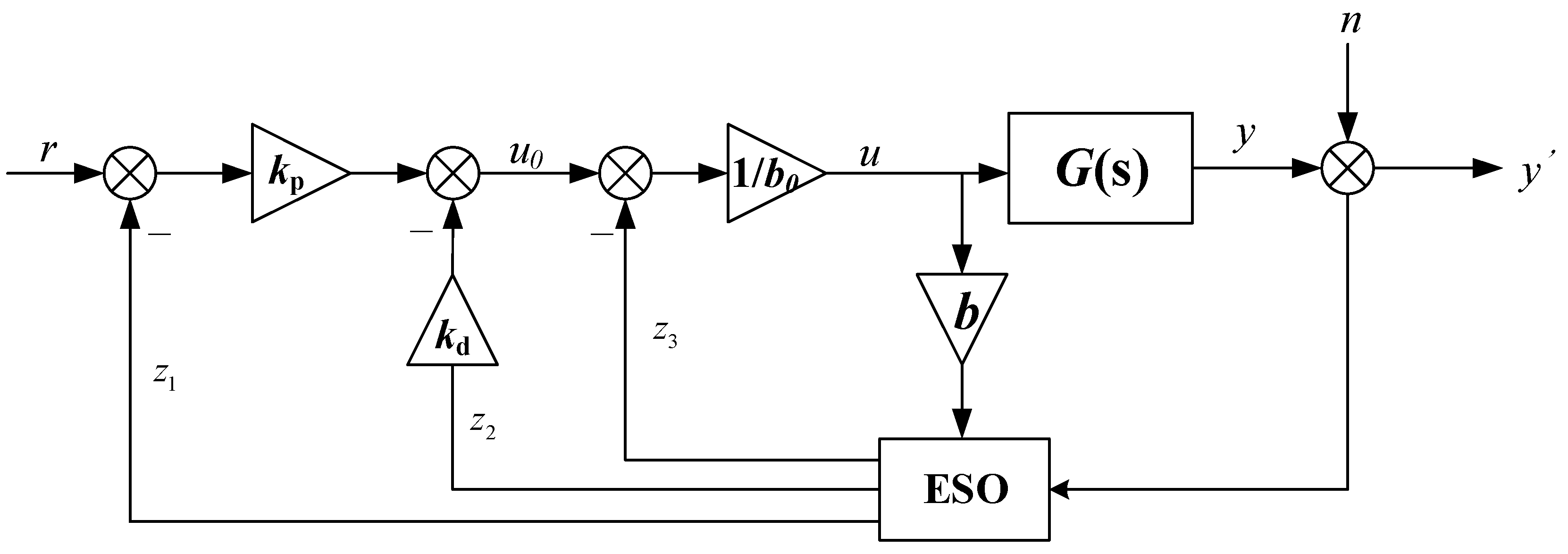
Figure 3 and Figure 4 show the ADRC structure in the presence of measurement noise at the measurement end, where y denotes the real output and y′ is the measurement. As we can see from figures, there are two inputs in the whole closed-loop systems: reference r and noise n. The factors affecting the control variables u are r and n. Besides, it is revealed in [34,35] that the ADRC is actually of two-degrees-of-freedom structure; therefore, we converted the above structure to the structure shown in Figure 5. For simplicity and generality, we define the transfer function from y to u as G_y(s) and the transfer function from r to u as G_r(s).

Converting the ADRC equations to the frequency domain using the Laplace transform, the control variable is

$$u(s)=G_r(s)r-G_y(s)\left(y+n\right)$$

(24)

As Figure 5 shows, the transfer function from n to u is equivalent to the transfer function from y to u. The comparison in noise reduction performance will be given by discussing the polynomials of G_y(s) between ADRC and MADRC.

3.2. Derivation of Transfer Function for ADRC

Based on the introduction of Section 3.1, this section will derive the transfer function from y to u for ADRC. Same as the controller described above, for the sake of universality and verifiability, the noise reduction conditions deduced later are not specific to any system or object. For clarity and simplicity, we will introduce the derivation process step by step.

(1)  Structural transformation for ESO:

As defined in (4), the conventional ESO structure is

$$\{\begin{array}{l}{\dot{z}}_1=z_2+{\beta }_1\left(y-z_1\right)\\ {\dot{z}}_2=z_3+bu+{\beta }_2\left(y-z_1\right)\\ {\dot{z}}_3={\beta }_3\left(y-z_1\right)\end{array}\Rightarrow \{\begin{array}{l}{\dot{z}}_1=-{\beta }_1{z}_1+z_2+{\beta }_{1}y\\ {\dot{z}}_2=-{\beta }_2{z}_1+z_3+bu+{\beta }_{2}y\\ {\dot{z}}_3=-{\beta }_3{z}_1+{\beta }_{3}y\end{array}$$

(25)

represented in matrix format,

$$\dot{z}=Az+B\overline{u}$$

(26)

where

$$\dot{z}=\left[\begin{array}{l}{\dot{z}}_1\\ {\dot{z}}_2\\ {\dot{z}}_3\end{array}\right]A=\left[\begin{array}{l}-{\beta }_{1}10\\ -{\beta }_{2}01\\ -{\beta }_{3}00\end{array}\right]z=\left[\begin{array}{l}{z}_1\\ z_2\\ z_3\end{array}\right]B=\left[\begin{array}{l}0{\beta }_1\\ b{\beta }_2\\ 0{\beta }_3\end{array}\right]\overline{u}=\left[\begin{array}{l}u\\ y\end{array}\right]$$

(27)

(2)  Laplace transformation for ESO, as follows:

The observer gain β are calculated from (6), as follows:

$$\{\begin{array}{l}{\beta }_1=3{\omega }_o\\ {\beta }_2=3{\omega }_o^2\\ {\beta }_3={\omega }_o^3\end{array}$$

(28)

and the estimates z₁, z₂, and z₃ are then deduced using the Laplace transform of (25) to yield

$$\{\begin{array}{l}{z}_1=\frac{bs}{d_1}u+\frac{(3{\omega }_o)s^2+(3{\omega }_o^2)s+{\omega }_o^3}{d_1}y\\ z_2=\frac{b{s}^2+(3b{\omega }_o)s}{d_1}u+\frac{(3{\omega }_o^2)s^2+{\omega }_o^{3}s}{d_1}y\\ z_3=\frac{{\omega }_o^3{s}^2}{d_1}y-\frac{b{\omega }_o^3}{d_1}u\end{array}$$

(29)

where

$$d_1=s^3+(3{\omega }_o)s^2+(3{\omega }_o^2)s+{\omega }_o^3$$

(30)

(3) Transfer function acquisition, as follows:

According to the control variable u expressed in (7) and (9),

$$u=\frac{1}{b}\left(k_{\mathrm{p}}\left(r-z_1\right)-k_{\mathrm{d}}{z}_2-z_3\right)$$

(31)

where the controller gain k_p and k_d are calculated from (20), as follows:

$$\{\begin{array}{l}{k}_{\mathrm{p}}={\omega }_c^2\\ k_{\mathrm{d}}=2{\omega }_c\end{array}$$

(32)

Meanwhile, from (20), u is deduced, as follows:

$$u=G_{r1}\left(s\right)r-G_{y1}\left(s\right)\left(y+n\right)=\frac{n_1}{d_2}r-\frac{n_2}{d_2}\left(y+n\right)$$

(33)

where G_r1(s) and G_y1(s) stand for transfer functions for ADRC with respective polynomials. Furthermore, G_y1(s) can be simplified as

$$G_{y1}\left(s\right)=\frac{N_1{s}^2+\left(3{\omega }_c^2{\omega }_o^2+2{\omega }_c{\omega }_o^3\right)s+{\omega }_c^2{\omega }_o^3}{d_2}$$

(34)

The detailed expression of the polynomials N₁, n₁, n₂, d₁, and d₂ in the transfer functions are given in Appendix A.

3.3. Derivation of Transfer Function for MADRC

The derivation of transfer function for MADRC is generally similar to that of ADRC; this section gives a brief description in order to avoid repetition and redundancy.

(1)  Structural transformation and Laplace transformation for ESO, as follows:

Similarly, the modified ESO structure (13) is

$$\{\begin{array}{l}{\dot{z}}_1=z_2+{\beta }_1\left(y-z_1\right)\\ {\dot{z}}_2=-a_1{z}_1-a_2{z}_2+bu+z_3+{\beta }_2\left(y-z_1\right)\\ {\dot{z}}_3={\beta }_3\left(y-z_1\right)\end{array}\Rightarrow \{\begin{array}{l}{\dot{z}}_1=-{\beta }_1{z}_1+z_2+{\beta }_{1}y\\ {\dot{z}}_2=\left(-a_1-{\beta }_2\right)z_1-a_2{z}_2+z_3+bu+{\beta }_{2}y\\ {\dot{z}}_3=-{\beta }_3{z}_1+{\beta }_{3}y\end{array}$$

(35)

The observer gain β are calculated from (15), as follows:

$$\{\begin{array}{l}{\beta }_1=3{\omega }_o-a_2\\ {\beta }_2=3{\omega }_o^2-3a_2{\omega }_o-a_1+a_2^2\\ {\beta }_3={\omega }_o^3\end{array}$$

(36)

The estimates z₁, z_2, and z₃ are then deduced using the Laplace transform of (35) to yield:

$$\{\begin{array}{l}{z}_1=\frac{(3{\omega }_o-a_2)s^2+(3{\omega }_o^2-a_1)s+{\omega }_o^3}{d_3}y+\frac{bs}{d_3}u\\ z_2=\frac{n_3}{d_3}y+\frac{b{s}^2+(3b{\omega }_o-a_{2}b)s}{d_3}u\\ z_3=\frac{{\omega }_o^3{s}^2+(a_2{\omega }_o^3)s+a_1{\omega }_o^3}{d_3}y-\frac{b{\omega }_o^3}{d_3}u\end{array}$$

(37)

(2) Transfer function acquisition, as follows:

The control variable u is expressed in (9) and (16), as follows:

$$u=\frac{1}{b}\left(k_{\mathrm{p}}\left(r-z_1\right)-k_{\mathrm{d}}{z}_2-\left(z_3-a_1{z}_1-a_2{z}_2\right)\right)$$

(38)

which is deduced as follows:

$$u=G_{r2}\left(s\right)r-G_{y2}\left(s\right)\left(y+n\right)=\frac{n_4}{d_4}r-\frac{n_5}{d_4}\left(y+n\right)$$

(39)

where G_r2(s) and G_y2(s) stand for transfer functions for MADRC. Furthermore, G_y2(s) can be simplified as

$$G_{y2}(s)=\frac{N_2{s}^2+n_6}{d_4}$$

(40)

The detailed expression of the polynomials N₂, n₃, n₄, n₅, n₆, d₃, and d₄ of the transfer functions are given in Appendix A.

3.4. Analysis of Noise Reduction Conditions

Before the analysis and proof on noise reduction performance, we have to clarify the following aspects:

• The noise discussed in this paper is usually the high-frequency noise in industrial applications, namely, ω is set to infinite;
• We consider the second-order system as a stable system, namely, a₁ > 0, a₂ > 0;
• The subject discussed in this paper is based on the condition that the observer and the controller bandwidths of the two types of ADRC (ω_o and ω_c) are equal.
• According to explicit point 1, when discussing the gain of the two kinds of ADRC with high-frequency noise, on the basis of the corresponding relation between frequency domain and complex domain G(jω) = G(s)|_{s = jω}, it becomes clear that the discussion focuses on the higher order terms of the transfer function, namely, the N₁ and N₂ in Formula (34) and (40).
• Assuming that the MADRC has the capability of noise reduction, N₂ must be less than N₁, that is to say, the inequality $N=N_1-N_2\ge 0$ should be proved.

For the point 5,

$$\begin{array}{lll}N& =& a_2^3-2a_2^2{\omega }_c-3a_2^2{\omega }_o+a_2{\omega }_c^2+6a_2{\omega }_c{\omega }_o+3a_2{\omega }_o^2\\ & & -2a_1{a}_2+2a_1{\omega }_c+3a_1{\omega }_o\\ & =& a_1{f}_1+a_2{f}_2(a_1>0,a_2>0)\end{array}$$

(41)

where

$$f_1=-2a_2+2{\omega }_c+3{\omega }_o$$

(42)

$$f_2={\left(a_2-{\omega }_c\right)}^2+3{\omega }_o^2+6{\omega }_c{\omega }_o-3a_2{\omega }_o$$

(43)

Since both a₁ and a₂ are positive, only f₁ and f₂ need to be discussed.

Note that f₁ > 0 as long as the following condition is satisfied:

$${\omega }_o\ge {\omega }_c\ge \frac{2}{5}{a}_2$$

(44)

Similarly, f₂ > 0, as long as the following condition is satisfied:

$${\omega }_o\ge {\omega }_c\ge \frac{1}{3}{a}_2$$

(45)

Combining condition (44) and condition (45), we get the following:

$${\omega }_o\ge {\omega }_c\ge \frac{2}{5}{a}_2$$

(46)

That is to say, as long as the condition ω_o ≥ ω_c ≥ 0.4a₂ is satisfied, the MADRC has a better noise reduction ability compared to the ADRC. For simplicity and generality, the condition is called the noise reduction condition hereinafter.

3.5. Reflections on the Condition

As shown in (46), the simplicity of the condition is beyond one’s expectation. Moreover, this is a very conservative or even stricter condition obtained by mathematical deduction. In other words, in practical control applications, this condition is extremely easy to meet:

(a)

In general, the observer bandwidth ω_o must be greater than the controller bandwidth ω_c, that is, the observer frequency must be greater than the controller operating frequency. Even in most ADRC applications, ω_o is ten times or even larger than ω_c;

(b)

On the other hand, the ADRC closed-loop characteristic polynomial is as follows:

$$s^2+2{\omega }_{c}s+{\omega }_c^2=0$$

(47)

and the open-loop characteristic polynomial of the plant is as follows:

$$s^2+a_{2}s+a_1=0$$

(48)

Obviously, since the closed-loop control response must be faster than the open-loop, namely, ω_c ≥ 0.5a₂. Even in the actual control, the closed-loop response is required to be much faster than the open-loop response: ω_c ≫ 0.5a₂.

To sum up, the strict condition obtained under the rigorous mathematical derivation is extremely easy to be satisfied in most control applications, and the margin of satisfaction is quite large.

This section completed the derivation of noise reduction condition of MADRC, and obtained a “strict noise reduction condition” that can be easily met in application. Through the theoretical parts of the Section 2 and Section 3, we have a preliminary understanding of the structure and noise reduction ability of MADRC. The next section will verify control quality of MADRC and noise reduction ability compared with ADRC through simulations and experiments.

4. Controller Design and Simulation

4.1. Model-Based System Identification

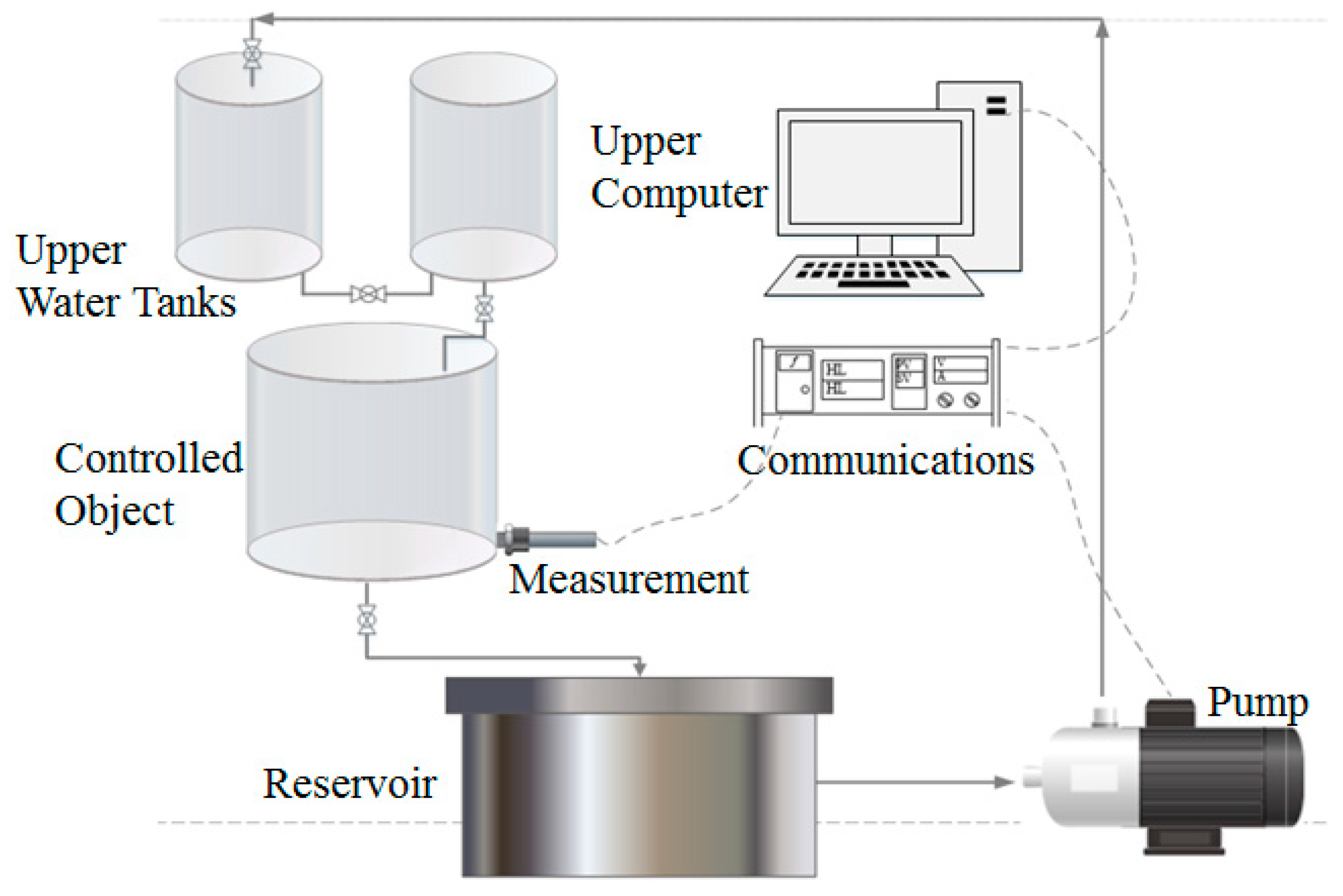
As introduced in the previous section, the water tank systems in industrial applications usually have large inertia. To this end, we have developed an experimental platform consisting of three water tanks whose structural diagram is shown in Figure 6. In order to emulate the large inertia, we have made full use of the inertia of the tank by making water flow through three water tanks in cascade.

The upper computer receives the signal of the communicator through the data bus. The communicator receives the signal of the pressure transducer and outputs the control signal to the frequency converter to adjust the rotational speed of the pump. The steady-state range of the controlled water level is obtained by testing at an operating point. Thus, the step-input experiment and the control experiment are carried out in the steady-state range. For simplicity and generality, the voltage signal received by the inverter is used as a control variable in the following description.

The form of transfer function of the platform is denoted as

$$G(s)=\frac{Y(s)}{U(s)}$$

(49)

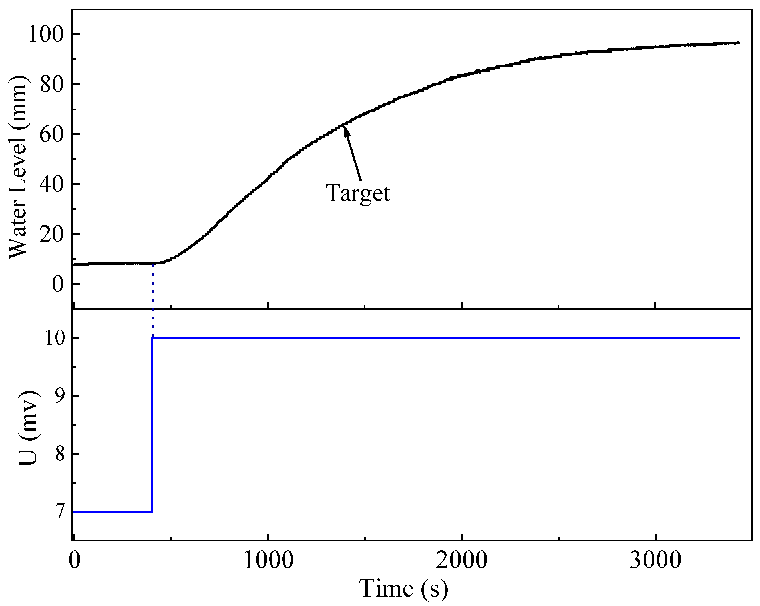
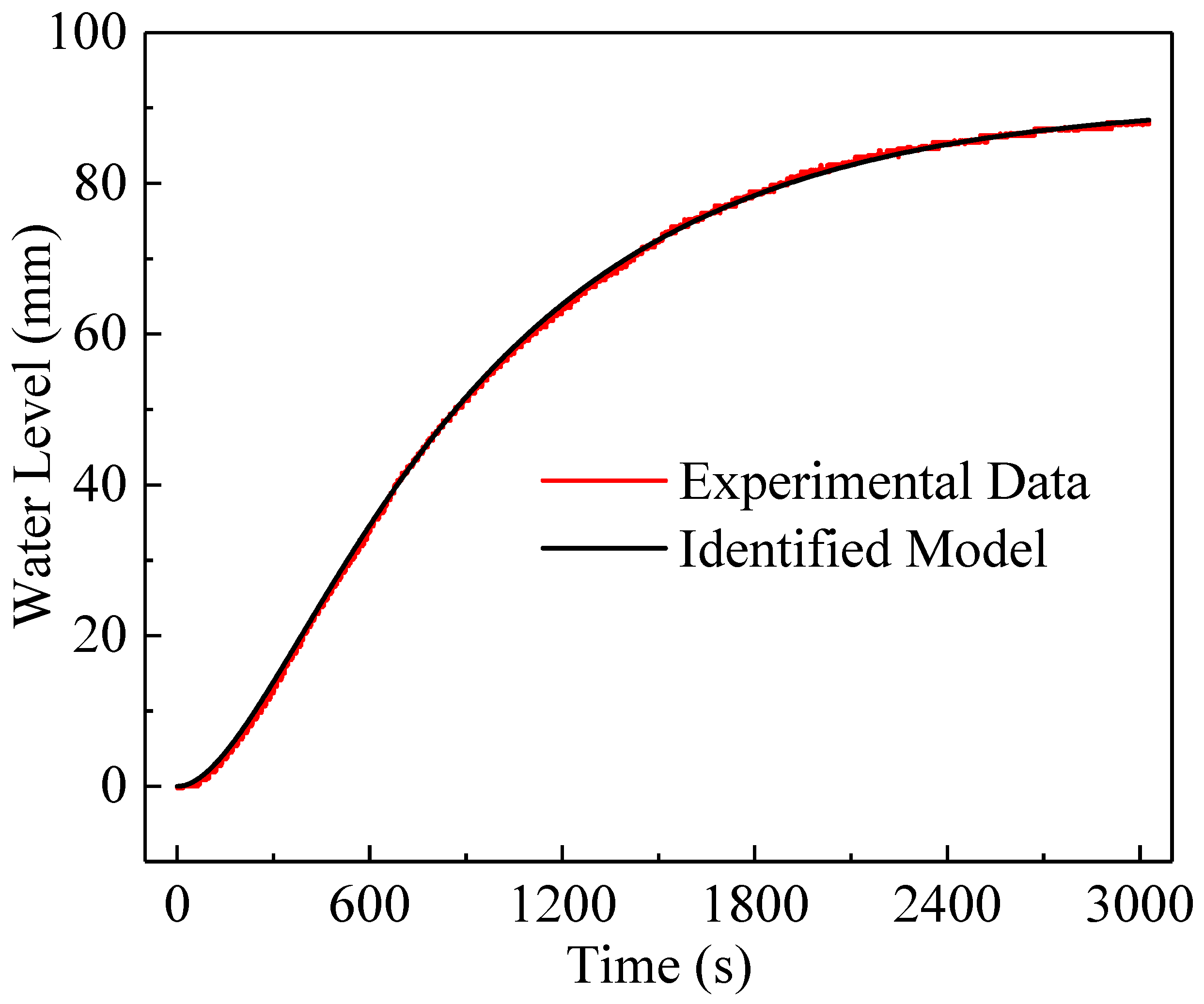
As mentioned above, U is the voltage signal received by the inverter and Y is the water level of the controlled plant. Figure 7 depicts the open-loop water level step response in the steady-state range, based on which the following transfer function was identified by using MATLAB System Identification Tool Box:

$$G=\frac{30.34}{\left(1+780.75s\right)\left(1+219.33s\right)}$$

(50)

Figure 8 shows the fitting of the experimental data with the identified model. According to the degree of fitting shown in the figure, it can be concluded that the identified transfer function represents the system very well. In addition, by comparing (10) and formula (50), it can be obtained that b = 1.77176 × 10⁻⁴, a₁ = 5.8397 × 10⁻⁶, and a₂ = 5.8401 × 10⁻³.

4.2. PI Controller Parameters Tuning

As empirical setting, the proportional-integral (PI) controller without differentiation is adequate to control the second-order system in industrial processes. Accordingly, we applied PI controller to the experiments. The form of PI controller is denoted as

$$G_c(s)=K_p+\frac{K_i}{s}$$

(51)

In order to design an engineering friendly controller for the system, we tuned the parameters based on the following method: SIMC-PID tuning rules widely used in industry, here SIMC means “Simple Internal Model Control” [36]. According to the identified result, the PI parameters are tuned as

$$K_p=0.070715,K_i=0.00008719$$

(52)

The PI control performance has fast response with good robustness, namely, fast transient period and reasonable overshoot, which will be further exhibited in Section 4.4.

4.3. ADRC Controller Parameters Tuning

According to the theoretical deduction above for ADRC, there is a quantitative relationship between derivative gain k_d and the damping factor ζ as shown in (23). Moreover, in order to compare the control performance between ADRC and MADRC, we set the ω_o and ω_c of the two types of ADRC to be equal to satisfy the unique variable principle.

In this experiment, the value of ω_o and ω_c are tuned as

$${\omega }_o=0.03,{\omega }_c=0.0035$$

(53)

On this basis, the parameters of ADRC and MADRC are as follows:

(1)

ADRC: β₁ = 0.09, β₂ = 2.7 × 10⁻³, β₃ = 2.7 × 10⁻⁵, k_p = 1.225 × 10⁻⁵, k_d = 7 × 10⁻³;

(2)

MADRC: β₁ = 0.08416, β₂ = 2.2026 × 10⁻³, β₃ = 2.7 × 10⁻⁵, k_p = 1.225 × 10⁻⁵, k_d = 7 × 10⁻³.

Obviously, since the improvement of ADRC mainly focuses on the ESO, the difference of parameters setting between ADRC and MADRC is mainly concentrated on the observer parameters β₁ and β₂, while the controller parameters are identical.

The superiority of MADRC is fully explicated in the following sections.

4.4. Simulation Comparison on Control Effects

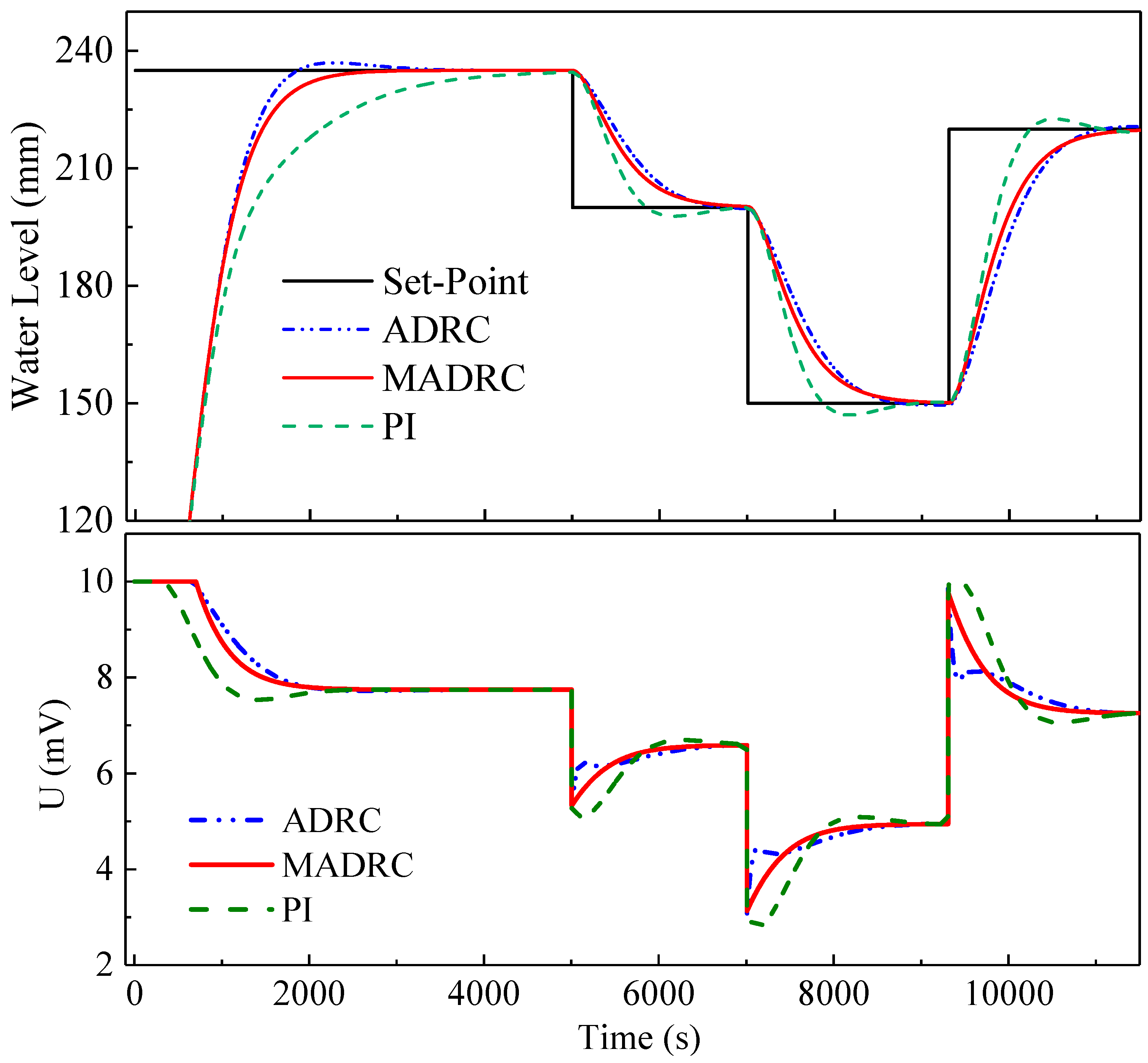
To evaluate and compare the robustness against parameter perturbation, PI, ADRC, and MADRC are simulated based on the identified model. Several sets of step-input experiments of water level are given to prove the validity of tuned parameters and the control effect of the MADRC compared with the ADRC and PI controller. The amplitude of control variable is limited within [0, 10], which considers the working voltage of actuator used in the experiment.

Figure 9 shows the result of reference tracking control. The step-changes in the water-level reference happened at 0 s, 5003 s, 7009 s, and 9310 s with amplitudes of +235, −35, −50, and +70, respectively. Compared with the PI and ADRC controller, the MADRC controller yields shorter transient period and smaller overshoot. It is generally known that such control performance is the goal of industrial control processes. From this point of view, the simulation results validate one of the capabilities of the MADRC mentioned above.

4.5. Noise Reduction Simulation Comparison

To compare and verify the capability of noise reduction, the ADRC and MADRC are simulated based on the identified model. High-frequency white noise is introduced into the close-loop to explore the influence of noise on the control variable. As mentioned above, the identified model is (50)

$$G\left(s\right)=\frac{30.34}{\left(1+780.75s\right)\left(1+219.33s\right)}$$

(54)

namely, the system parameter a₂ = 5.84 × 10⁻³ in the second-order system (10). We adopted the same controller parameters of ADRC and MADRC, i.e., ω_o = 0.03 and ω_c = 0.0035, which satisfy the noise reduction condition ω_o ≥ ω_c ≥ 0.4a₂.

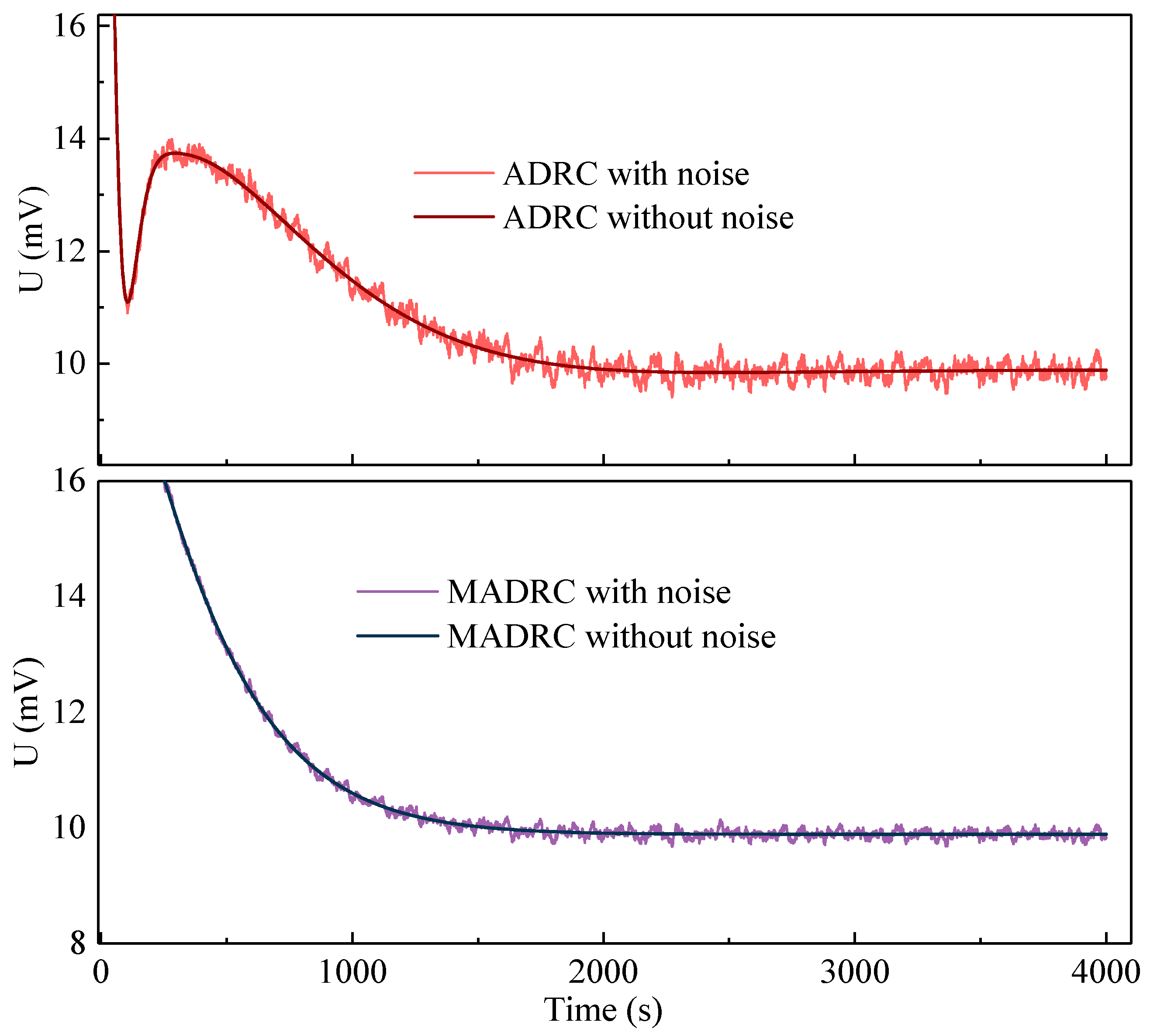
Figure 10 and Figure 11 show the result of noise-reduction simulation experiments. Figure 10 shows the output values of the two ADRC step experiments in the presence of noise, and highlights the fluctuation of output values after introducing white noise.

Figure 11 shows the fluctuation of control variables of the two ADRC relative to their noise-free conditions. Since the settings of the horizontal and vertical coordinates of the two figures are the same, it can be seen intuitively that the fluctuation of output control variable is much smaller in the MADRC than in the ADRC. This preliminarily verifies the idea proposed in this paper, that is, the MADRC has a better noise reduction ability compared with the ADRC under the same noise interference and the same bandwidth settings.

In order to demonstrate the noise reduction ability of the MADRC quantitatively, we introduced the integral absolute error (IAE) to evaluate the fluctuations of control variable, which is defined as

$$IAE={\displaystyle {\int }_0^T\left|y-r\right|dt}$$

(55)

In this experiment, y denotes the control variable under noise and r denotes noise-free reference. Obviously, the smaller the IAE, the smaller the fluctuation. Calculation results of the two ADRC are as follows:

• ADRC:

  $$IA{E}_{ADRC}=449.9305$$

  (56)
• MADRC:

  $$IA{E}_{MADRC}=223.0452$$

  (57)

By comparing (56) and (57), IAE_MADRC < IAE_ADRC, and we can draw the same conclusion that MADRC indeed has a better noise reduction ability.

So far, the validity and feasibility of the proposed MADRC have been demonstrated by simulation experiments with the identified model. Therefore, the prerequisite for the hardware experiment is readily met. The water pump control experiment in hardware will be carried out in the next section.

5. Experimental Results

5.1. Experimental Setup

The picture of water pump control experimental platform is shown in Figure 12, where some critical equipments are labeled. To avoid distraction, some irrelevant components in the experiment, such as lift of pump, pipe diameter, relays, and opening of each valve, are not detailed in the figure, but they are indispensable for the experiment.

The experimental scheme is to change the rotational speed of the pump by adjusting the input control signal of the variable frequency pump, so as to adjust the flow of water, and then adjust the water level of the tank. It needs to be emphasized that the factors affecting the water level of the tank are not only the inlet water volume but also its own water level, because the increase of the water level will lead to the increase of the output water yield.

The host computer controls the system, and the control algorithm is realized by building control module structures and tuning parameters. The communication between the platform and the host computer is via MODBUS module.

5.2. Experimental Results

Based on the previous simulation work in Section 4, we applied the well-tuned controller parameters to control the water level of the experimental platform. In order to verify the quantitative relationship between k_d and ζ and take T_s into account, k_d is set in discrete steps. The other parameters and the structure of the controllers are the same as mentioned in the simulation experiment. In order to fully reflect the effect of the controller, the experiments were set up with multiple groups of positive/negative steps in different amplitudes. Figure 13 and Figure 14 represent the water level tracking performance of ADRC and MADRC controllers, respectively.

Similarly, in order to demonstrate the control effect more quantitatively, we introduced some evaluation indices, such as integral absolute error per time, IAE_T, overshoot O, and transient time T_s with 2% error band.

The definition of IAE_T is

$$IA{E}_T=\frac{{\displaystyle {\int }_0^T\left|y-r\right|dt}}{T}$$

(58)

where y and r denote the actual water level and set point, respectively.

The overshoot is defined as

$$O=\frac{\left(y_{\max }-y_{t=\infty }\right)}{y_{t=\infty }}\times 100\%$$

(59)

where y_max denotes maximum output value and y_{t = ∞} is the stable value.

The definition of transient time is the time required for the response curve to reach and stay within a range of certain percentage (usually 2% or 5%) of the final value [34]. The error band is the range between the ±2%/±5% amplitude around the reference value.

Each of the three evaluation indices focuses on different aspects. The transient time T_s is a comprehensive index reflecting the response speed and damping degree of the system. Simply speaking, it can be considered as the minimum time required to complete the specified control function. The overshoot is the most commonly used control index to partially depict the robustness of a controller. In some specific industrial processes, the overshoot is strictly restricted to nearly zero; IAE_T is an auxiliary evaluation index in this paper. It represents the real-time error between the actual output value and the reference value, which is used to indicate the accuracy of the control performance.

The calculation results of evaluation indices are tabulated in

Table 1. Evaluation indices.

	Controller	Step 1: +30 (0–30 mm)		Step 2: +30 (30–60 mm)		Step 3: −30 (60–30 mm)		Step 4: +55 (30–85 mm)		Step 5: −60 (85–25 mm)
Index		ADRC	MADRC	ADRC	MADRC	ADRC	MADRC	ADRC	MADRC	ADRC	MADRC
Ts (Error Band: 2%)		2181.4 s	2052 s	2094.8 s	1359 s	2157.8 s	968 s	2332.4 s	1506.8 s	2140.6 s	1364 s
Overshoot (O)		10.17%	9.07%	7.33%	4.03%	6.67%	0.80%	3.96%	1.18%	5.95%	2.48%
IAET		5.8258	9.872	6.5226	8.3018	7.1263	9.6148	13.2314	13.323	11.6147	11.1421

. In the next section, the analysis will be carried out according to the evaluation indicators in the table.

5.3. Result Analysis

According to the values in Table 1, it is obvious that T_s and overshoot is smaller in MADRC than in ADRC in each step experiment, which reflects the excellent control performance of the MADRC compared with the ADRC in terms of water pump control. As for IAE_T, the IAE_T of the ADRC is less than that of the MADRC in smaller steps and almost equal in larger steps. Reasons for this can be the overshoot of the ADRC is similar to that of the MADRC when the step is small, but the rising speed of the ADRC controlled signal is faster than that of the MADRC, thus leading to smaller real-time error. During large steps, although the ADRC is more powerful than the MADRC, the overshoot of the ADRC is also larger than that of the MADRC, so the IAE_T of the ADRC and the MADRC become almost the same.

The comparison of control performance in the above analysis can be observed in the figures. Overall, the MADRC has an excellent control performance compared to the ADRC in terms of water pump control, showing great potential in its application to water pump control in industrial processes.

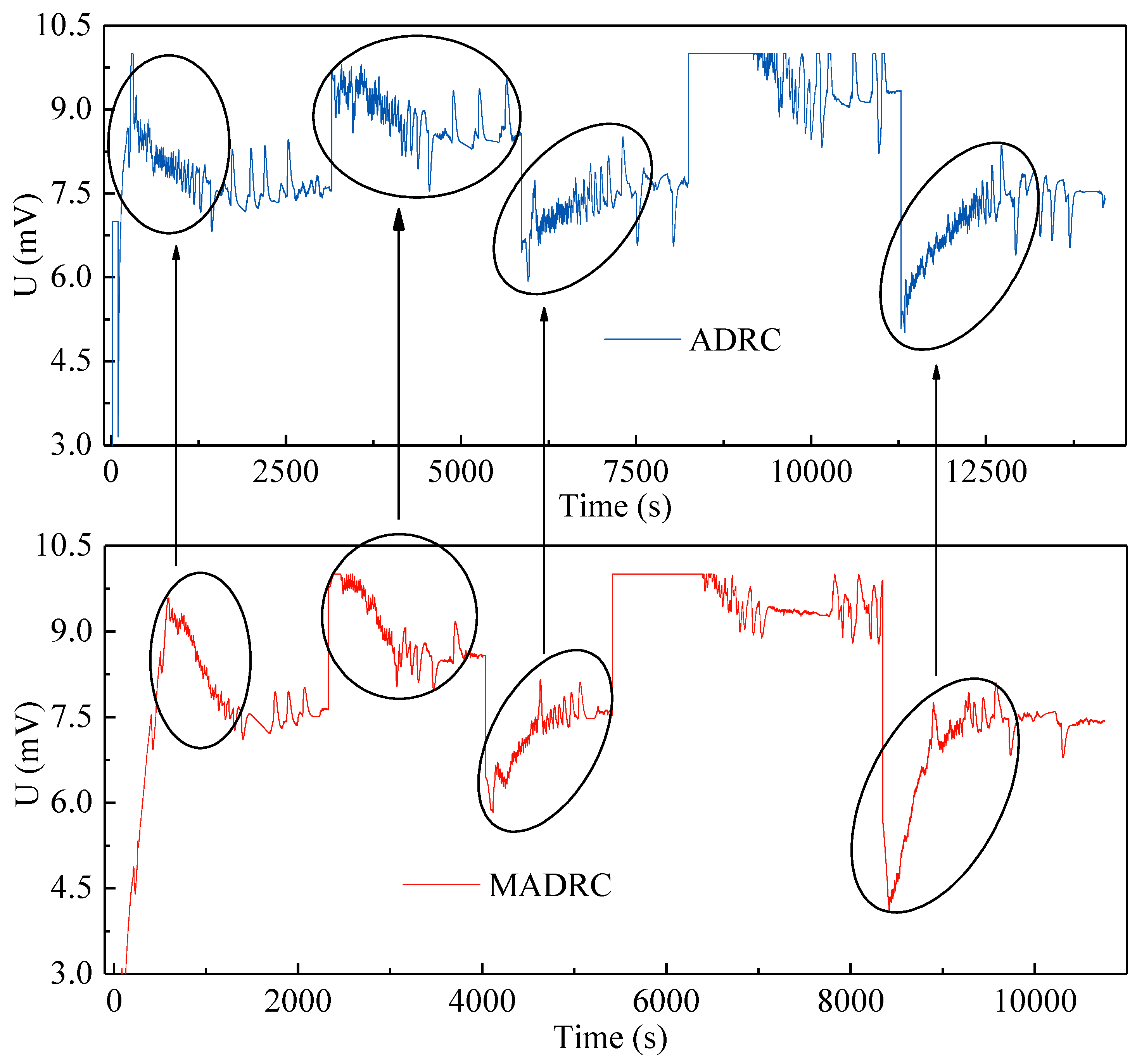
Noise reduction analysis is achieved mainly through the comparison of the ADRC and MADRC control variables, namely, the output signal of the pump speed. Since the two sets of experiments have the same step amplitudes, it is feasible to compare the control variables. Figure 15 shows the comparison of control variables.

Valuable insights can be obtained from the experimental results: when we have to deal with some objects with the attributes of slow dynamics, strong nonlinearity, and various disturbances, MADRC is indeed a trustworthy choice, which can effectively deal with various uncertainties. Meanwhile, its noise reduction performance is advantageous to various executing agencies in industry, especially mechanical equipment. All in all, MADRC has excellent application prospects in the field of industrial process control.

It clearly depicted in Figure 15 that when control variable undergoes a large numerical change, severe fluctuation will occur. However, according to the corresponding circled plots, it is obvious that the fluctuation of control variable is smaller for the MADRC than for the ADRC. Moreover, on the basis of model information and controller parameters, the parameters satisfy the noise reduction conditions mentioned in this paper: ω_o ≥ ω_c ≥ 0.4a₂. This shows that the MADRC indeed has a better noise reduction capability compared with the ADRC under the same noise reduction condition. As in the simulation experiments, the feasibility of the noise reduction condition is also demonstrated, which is quite useful in industrial applications for its friendliness to actuators.

6. Conclusions

This paper verifies the promising application of the modified model-assisted ADRC control methodology on a practical water pump control system by analysis, simulation, and well-designed hardware experiment. This paper focuses on the tracking performance and noise reduction capability of the MADRC. The superiority of the MADRC in these two aspects has been verified by simulation and practical hardware experiment.

On the one hand, the MADRC has better control performance, especially in the reference tracking with large step changes. It can be clearly seen from the simulation results in Figure 9 and the actual experimental results in Table 1 that MADRC is superior to ADRC and PID in both overshoot and transient time. Specifically, in the case of a smaller overshoot, it also has faster transient time, which is essential for the control process under specific requirements.

On the other hand, the MADRC has better noise reduction capability compared to the ADRC under the same noise reduction condition. Furthermore, the strict condition derived under the rigorous mathematical analysis is extremely easy to satisfy in the most practical control processes, and the satisfactory margin is quite large. The control variables with weakened fluctuation after noise reduction will benefit the actuator and prolong its life, which is especially critical for systems with complex installation procedure.

To sum up, the proposed MADRC method is able to achieve a better control performance and better noise reduction capability by sacrificing some structure conciseness and ease of use.

This paper provides a hybrid data-driven and model-assisted active disturbance rejection control for precise control of water level in industrial process, and it could even be carried out in extensive industrial control problems. More importantly, this paper provides an idea of designing control algorithm: by combining model information with real-time input and output data, better control effects could be achieved by using both steady state data and dynamic data in the control process. Moreover, the best disturbance-rejection performance of the MADRC control approach can contribute to pumped-storage distributed energy-supply systems like combined cooling, heating and power-generating systems [37] and also to a study on robust optimization of the distributed generating units [38] in the future.

References

- Ullah, I.; Kim, D. An Optimization Scheme for Water Pump Control in Smart Fish Farm with Efficient Energy Consumption. Processes 2018, 6, 65. [Google Scholar] [CrossRef]
- Rinas, M.; Tränckner, J.; Koegst, T. Sedimentation of Raw Sewage: Investigations for a Pumping Station in Northern Germany under Energy-Efficient Pump Control. Water 2019, 11, 40. [Google Scholar] [CrossRef]
- Carravetta, A.; Antipodi, L.; Golia, U.; Fecarotta, O. Energy Saving in a Water Supply Network by Coupling a Pump and a Pump as Turbine (PAT) in a Turbopump. Water 2017, 9, 62. [Google Scholar] [CrossRef]
- Hu, K.; Pan, F.; Sun, L.; Li, D.; Lee, K.Y. On Tuning and Practical Implementation of Active Disturbance Rejection Controller: A Case Study from a Regenerative Heater in a 1000 MW Power Plant. Ind. Eng. Chem. 2016, 55, 6686–6695. [Google Scholar]
- Pawlak, M. Active Fault Tolerant Control System for the Measurement Circuit in a Drum Boiler Feed-Water Control System. Meas. Control 2018, 51, 4–15. [Google Scholar] [CrossRef]
- Mystkowski, A.; Kierdelewicz, A. Fractional-Order Water Level Control Based on PLC: Hardware-In-The-Loop Simulation and Experimental Validation. Energies 2018, 11, 2928. [Google Scholar] [CrossRef]
- Join, C.; Robert, G.; Fliess, M. Model-Free Based Water Level Control for Hydroelectric Power Plants. IFAC Proc. Vol. 2010, 43, 134–139. [Google Scholar] [CrossRef] [Green Version]
- Guo, W.; Wang, B.; Yang, J.; Xue, Y. Optimal control of water level oscillations in surge tank of hydropower station with long headrace tunnel under combined operating conditions. Appl. Math. Model. 2017, 47, 260–275. [Google Scholar] [CrossRef]
- Safarzadeh, O.; Khaki-Sedigh, A.; Shirani, A. Identification and robust water level control of horizontal steam generators using quantitative feedback theory. Energy Convers. Manag. 2011, 52, 3103–3111. [Google Scholar] [CrossRef]
- Ansarifar, G.; Talebi, H.; Davilu, H. Adaptive estimator-based dynamic sliding mode control for the water level of nuclear steam generators. Prog. Nucl. Energy 2012, 56, 61–70. [Google Scholar] [CrossRef]
- Salehi, A.; Safarzadeh, O.; Kazemi, M.H. Fractional order PID control of steam generator water level for nuclear steam supply systems. Nucl. Eng. Des. 2019, 342, 45–59. [Google Scholar] [CrossRef]
- Salehi, A.; Kazemi, M.H.; Safarzadeh, O. The μ-synthesis and analysis of water level control in steam generators. Nucl. Eng. Technol. 2019, 51, 163–169. [Google Scholar] [CrossRef]
- Riccardo, V.; Luca, R. Overshoots in the water-level control of hydropower plants. Renew. Energy 2019, 131, 800–810. [Google Scholar]
- Na, M.G.; Sim, Y.R.; Lee, Y.J. Design of an adaptive predictive controller for steam generators. IEEE Trans. Nucl. Sci. 2003, 50, 186–193. [Google Scholar]
- Rust, J.H. Nuclear Power Plant Engineering, 2nd ed.; S.W. Holland: Atlanta, GA, USA, 1979. [Google Scholar]
- Na, M.G. Auto-tuned PID controller using a model predictive control method for the steam generator water level. IEEE Trans. Sci. 2001, 48, 1664–1671. [Google Scholar] [Green Version]
- Han, J. From PID to Active Disturbance Rejection Control. IEEE Trans. Ind. Electron. 2009, 56, 900–906. [Google Scholar] [CrossRef]
- Roman, R.-C.; Precup, R.-E.; Petriu, E.M.; Dragan, F. Combination of Data-Driven Active Disturbance Rejection and Takagi-Sugeno Fuzzy Control with Experimental Validation on Tower Crane Systems. Energies 2019, 12, 1548. [Google Scholar] [CrossRef]
- Zhang, H.; Liu, X.; Ji, H.; Hou, Z.; Fan, L. Multi-Agent-Based Data-Driven Distributed Adaptive Cooperative Control in Urban Traffic Signal Timing. Energies 2019, 12, 1402. [Google Scholar] [CrossRef]
- Roman, R.-C.; Radac, M.-B.; Precup, R.-E.; Petriu, E.M. Virtual Reference Feedback Tuning of Model-Free Control Algorithms for Servo Systems. Machines 2017, 5, 25. [Google Scholar] [CrossRef]
- Veronesi, M.; Visioli, A. Deterministic Performance Assessment and Retuning of Industrial Controllers Based on Routine Operating Data: Applications. Processes 2015, 3, 113–137. [Google Scholar] [CrossRef] [Green Version]
- Li, S.; Li, J. Output Predictor-Based Active Disturbance Rejection Control for a Wind Energy Conversion System with PMSG. IEEE Access 2017, 5, 5205–5214. [Google Scholar] [CrossRef]
- Hou, Y.; Gao, Z.; Jiang, F.; Boulter, B.T. Active disturbance rejection control for web tension regulation. IEEE CDC Conf. 2001, 5, 4974–4979. [Google Scholar]
- Su, Y.; Duan, B.; Zheng, C.; Zhang, Y.; Chen, G.; Mi, J. Disturbance-Rejection High-Precision Motion Control of a Stewart Platform. IEEE Trans. Control Syst. Technol. 2004, 12, 364–374. [Google Scholar] [CrossRef]
- Yang, J.; Chen, W.-H.; Li, S.; Guo, L.; Yan, Y. Disturbance/Uncertainty Estimation and Attenuation Techniques in PMSM Drives—A Survey. IEEE Trans. Ind. Electron. 2017, 64, 3273–3285. [Google Scholar] [CrossRef]
- Madoński, R.; Herman, P. Survey on methods of increasing the efficiency of extended state disturbance observers. ISA Trans. 2015, 56, 18–27. [Google Scholar] [CrossRef]
- Sun, L.; Hua, Q.; Shen, J.; Xue, Y.; Li, D.; Lee, K.Y. Multi-objective optimization for advanced superheater steam temperature control in a 300 MW power plant. Appl. Energy 2017, 208, 592–606. [Google Scholar] [CrossRef]
- Song, K.; Hao, T.; Xie, H. Disturbance rejection control of air–fuel ratio with transport-delay in engines. Control Eng. Pract. 2018, 79, 36–49. [Google Scholar] [CrossRef]
- Dong, J.; Sun, L.; Li, D.; Lee, K.Y. A Practical Multivariable Control Approach Based on Inverted Decoupling and Decentralized Active Disturbance Rejection Control. Ind. Eng. Chem. 2016, 55, 2008–2019. [Google Scholar]
- Sun, L.; Li, D.; Gao, Z.; Yang, Z.; Zhao, S. Combined feedforward and model-assisted active disturbance rejection control for non-minimum phase system. ISA Trans. 2016, 64, 24–33. [Google Scholar] [CrossRef]
- Sun, L.; Shen, J.; Hua, Q.; Lee, K.Y. Data-driven oxygen excess ratio control for proton exchange membrane fuel cell. Appl. Energy 2018, 231, 866–875. [Google Scholar] [CrossRef]
- Zheng, Q.; Chen, Z.; Gao, Z. A practical approach to disturbance decoupling control. Control Eng. Pract. 2009, 17, 1016–1025. [Google Scholar] [CrossRef] [Green Version]
- Gao, Z. Scaling and bandwidth-parameterization based controller tuning. Proc. Am. Control Conf. 2003, 6, 4989–4996. [Google Scholar]
- Yang, J.; Li, S.; Yu, X. Sliding-Mode Control for Systems with Mismatched Uncertainties via a Disturbance Observer. IEEE Trans. Ind. Electron. 2013, 60, 160–169. [Google Scholar] [CrossRef]
- Xue, W.; Bai, W.; Yang, S.; Song, K.; Huang, Y.; Xie, H.; Yi, H. ADRC With Adaptive Extended State Observer and its Application to Air–Fuel Ratio Control in Gasoline Engines. IEEE Trans. Ind. Electron. 2015, 62, 5847–5857. [Google Scholar] [CrossRef]
- Skogestad, S. Simple analytic rules for model reduction and PID controller tuning. J. Process Control 2003, 13, 291–309. [Google Scholar] [CrossRef] [Green Version]
- Chen, C.; Lin, J.; Pan, L.; Lee, K.Y.; Sun, L. Improving Simultaneous Cooling and Power Load-Following Capability for MGT-CCP Using Coordinated Predictive Controls. Energies 2019, 12, 1180. [Google Scholar] [CrossRef]
- Peng, C.; Xu, L.; Gong, X.; Sun, H.; Pan, L. Molecular Evolution Based Dynamic Reconfiguration of Distribution Networks With DGs Considering Three-Phase Balance and Switching Times. IEEE Trans. Ind. Inf. 2019, 15, 1866–1876. [Google Scholar] [CrossRef]
Figure 1.
The block diagram of the second-order active disturbance rejection control ADRC.
Figure 2.
The modified active disturbance rejection control (MADRC) block diagram for the second-order system.
Figure 3.
The ADRC block diagram with measurement noise.
Figure 4.
The MADRC block diagram with measurement noise.
Figure 5.
Block diagram of the system for ADRC.
Figure 6.
Structural diagram of the water tanks platform.
Figure 7.
Open-loop step response.
Figure 8.
The fitting of experimental data with the identified model.
Figure 9.
Simulation of reference tracking. Steps occur at 0 s, 5003 s, 7009 s, and 9310 s.
Figure 10.
Simulation of noise reduction and the fluctuation of output values.
Figure 11.
The fluctuations of control variables of the two ADRC.
Figure 12.
Photo of water pump experimental platform.
Figure 13.
Water level tracking experiment with conventional ADRC controller.
Figure 14.
Water level tracking experiment with MADRC controller.
Figure 15.
Comparison of control variable fluctuations.