Robustness Spatiotemporal Clustering and Trend Detection of Rainfall Erosivity Density in Greece

Abstract

Soil erosion is affected by rainfall, among other factors, and it is likely to increase in the future due to climate change impacts, resulting in higher rainfall intensities. This paper evaluates the impact of the missing values ratio on the computation of the rainfall erosivity factor, R, and erosivity density, ED. The paper also investigates the temporal trends and defines regions of Greece with a similar monthly distribution of ED using an unsupervised method. Preprocessed and free from noise and errors rainfall data from 108 stations across Greece were extracted from the Greek National Bank of Hydrological and Meteorological Information. The rainfall data were analyzed and erosive rainfalls were identified, their return period was determined using intensity–duration–frequency curves and R and ED values were computed. The impact of missing data in the computation of annual values of R and ED was investigated using a Monte Carlo simulation. The findings indicated that missing rainfall data resulted in a linear underestimation of R, while ED is more robust. The trends in ED timeseries were evaluated using the Kendall’s Tau test and their autocorrelation and partial autocorrelation were computed for a small subset of stations using criteria based on the quality of data. Furthermore, cluster analysis was applied to a larger subset of stations to define regions of Greece with similar monthly distribution of ED. The findings of this study indicate that: (a) ED should be preferred for the assessment of erosivity in Greece over the direct computation of R, (b) ED timeseries are found to be stationary for the majority of the selected stations, in contrast to reported precipitation trends for the same time period, (c) Greece is divided into three clusters/areas of stations with distinct monthly distributions of ED.

1. Introduction

It is plausible that future climate change would increase the intensity of rainfall in Europe, as indicated by the European research project EURO-CORDEX [1]. This expected increase in rainfall intensity will result in increased potential soil erosion rates [2]. Major parts of Greece are affected by desertification due to a combination of their bio-geoclimatic characteristics and the overexploitation and misuse of natural resources [3]. Since the most significant process responsible for soil loss is related to rainfall intensity, any possible increase of future rainfall intensity will directly affect and intensify this desertification process [4].

The difficulty of modeling the relationship of the distribution of the raindrop sizes to the detachment of soil particles has led to the employment of more conventional and accessible rainfall indicators, such as those based on rainfall intensities. The Universal Soil Loss Equation, USLE [5], and its computerized revisions RUSLE [6] and RUSLE2 [7] have been used worldwide, and one of its empirically based factors, rainfall erosivity $R$, is based on rainfall intensities. USLE has the form:

$$A=R\times K\times L\times S\times C\times P$$

(1)

where $A$ is the long-term (i.e., over 20 years), average rate of soil loss (t∙ha⁻¹∙year⁻¹) that is associated with sheet and rill erosion, $R$ is the rainfall erosivity factor (MJ∙mm∙ha⁻¹∙h⁻¹∙year⁻¹), $K$ is the soil erodibility factor (t∙h∙MJ⁻¹∙mm⁻¹), $L$ and $S$ are the slope length and steepness factors, C is a cover-management factor and P is a supporting practices factor. The second revised version of USLE, RUSLE2, introduced erosivity density ($ED$), as a measure of rainfall erosivity per unit rainfall. $ED$ was proposed in order to develop $R$ values for the USA on a monthly basis and a given location, due to the fact that $ED$ requires shorter record lengths, as 10 years lead to acceptable results; also because it allows more missing data than $R$ and is independent of the elevation.

Concerning the $ED$ values in Greece, Panagos et. al. [8] used interpolated values of $R$ and also interpolated monthly precipitation, both coming from different origins, to produce maps of seasonal $ED$ values, and plotted the average values per three decades and the nine-year moving average for 8 stations. However, surveys [9,10] of the above pluviograph data revealed significant proportions of missing values that affect the calculations of $R$. Also, the rainfall energy equation that was used, coming from the Revised Universal Soil Loss Equation, RUSLE [6], was developed for an application concerning re-ordered rainfall intensity data and not natural rainfall data [11] and as a consequence it significantly underestimated $R$ [12]. Last but not least, the difference between erosivity calculated from fixed interval and not breakpoint data was not taken into account as it was by the developers of RUSLE2 [7,13].

Precipitation in Greece has been investigated in several studies over the past two decades [14,15,16,17,18]. In general, precipitation varies from its maximum values during winter to a minimum during summer. Detection of $ED$ trends in Greece is related to an analogous problem concerning precipitation trends. The latter problem has also been dealt with in the literature. Annual precipitation presents a downward trend for the period 1955–2001 [14] and the mean annual rain intensity shows both statistically significant negative trends mainly in the west sub-regions, and positive trends in the wider area of Athens, the complex of Cyclades Islands, Crete and north-eastern sub-regions for the period 1962–2002 [19]. A more recent study [20] using data from 1940 to 2012 showed that changes occurred at different scales, with annual rainfall being stable for the last 15 years. The same study used clustering methods to create eight regions with similar climatic properties. Another study concerning the spatial variation of rainfall in Greece showed that a clear contrast exists in the country between the drier, eastern and the western part of the country, which experiences more rainfall [21].

The determination of monthly temporal distribution patterns of $ED$, or the categorization of these data into meaningful clusters, where no output information exists, belongs to the domain of unsupervised learning [22]. A large number of these learning methods exist in the literature and a classification of them is presented by Sheikholeslami et al. [23]. In practice, the most common ones used are k-means [24,25] and Hierarchical Clustering [26]. The optimal number of clusters in unsupervised learning, which is initially unknown, is a major issue because different algorithms, or even a single algorithm with different parameters, produce different clusters of data. As a result, a number of methods have been developed for the determination of the optimal number of clusters. Many of them use the concept of relative cluster validity [27], where results from different clustering methods are compared using a predefined metric. A number of these methods can be found in Milligan et al. [28] and a comprehensive list of 30 different indices can be found in Charrad et al. [29]. Three popular methods are: (a) the elbow rule, which is a visual, sometimes ambiguous, method, (b) the silhouette index [30] that measures how well data are contained within clusters and (c) the “gap” statistic [31] that uses the output of a clustering algorithm and compares the observed within-cluster variation to the one that has data with a uniform distribution.

In view of the above considerations, this study aims firstly to assess the impact of the missing values ratio to the computation of $R$ and $ED$ values in a numerical way, as RUSLE2 included a theoretical justification. This first part of the study is necessary in order to justify the intermediate step of calculations of $ED$, which permits the utilization of coarser precipitation data that are more abundant in comparison to denser pluviograph data. In the sequel, the objective of the present study is to investigate $ED$ temporal trends in Greece using the latest methodologies developed and presented with RUSLE2, taking account of the presence of missing values in precipitation records. Finally, the study attempts to determine the presence of clusters, their optimal number and consequently to define regions in Greece that have a similar monthly distribution of ED. The proposed clustering analysis is performed in an unsupervised way and it has not appeared in the literature for the specific problem. An earlier, shorter, version of this paper, without the clustering analysis and only annual values calculations and analysis, was presented in the 3rd WATER Electronic Conference on Water Sciences (ECWS-3) [32].

2. Materials and Methods

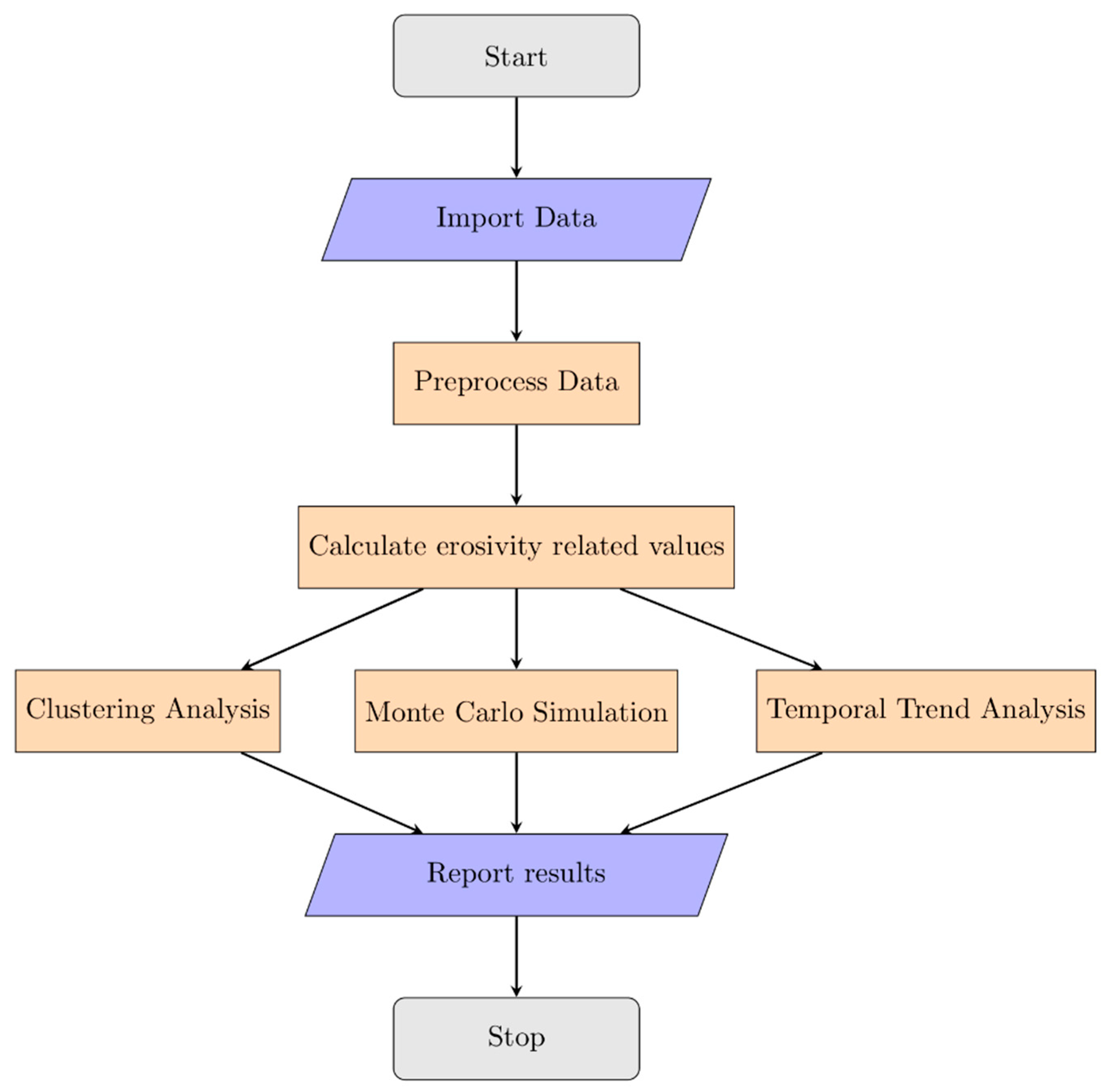
The methodology that was applied in the study is presented in Figure 1 as a flowchart. High frequency precipitation data were imported and preprocessed, erosivity and erosivity density values were calculated and a number of procedures were used in order to analyze the latter.

2.1. Data Acquisition and Processing

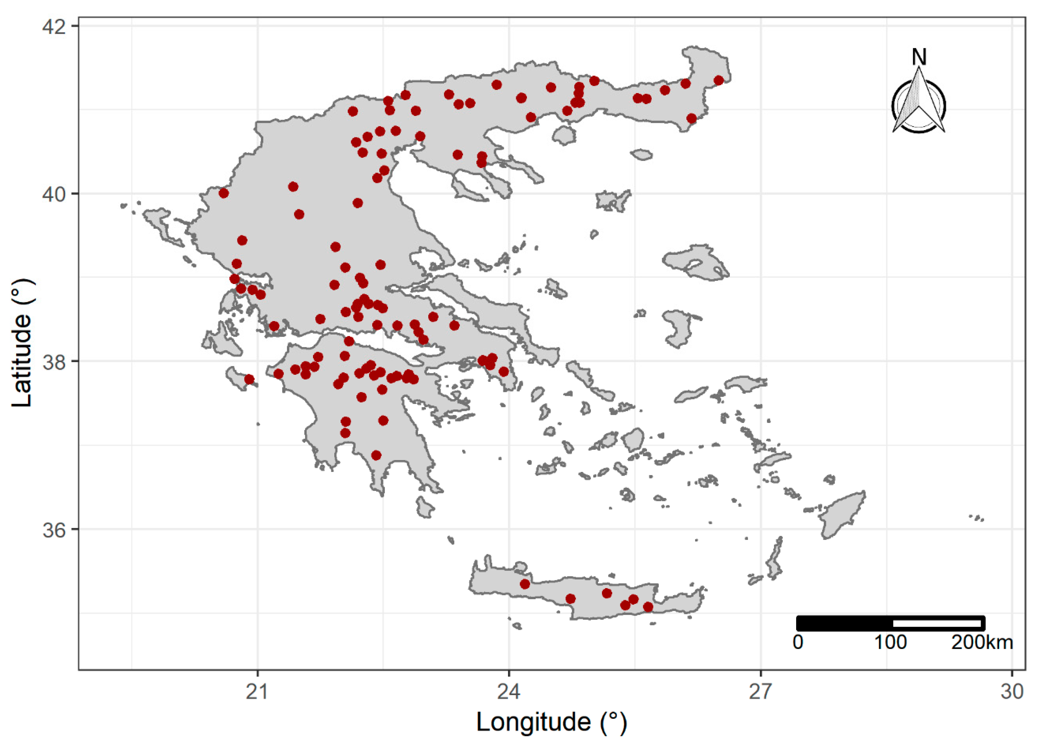
The data used in the analysis were taken from the Greek National Bank of Hydrological and Meteorological Information [33] for 108 meteorological stations across Greece (Figure 2). The time series comprised a total of 2447 years of 30-minute-records and 478 years of five-minute-records for the time period from 1953 to 1997, with a mean length of 26.6 years per station. The time series were checked for consistency and errors as follows: (a) in records of repetitive values near zero (i.e., ≤0.01 mm), these values were set to zero and (b) records of aggregated values, where the time step was larger than the reported, were removed. The pluviograph data coverage was 43.2% on average.

The product of the kinetic energy of a rainfall and its maximum 30 min intensity, $E{I}_{30}$ (MJ.mm/ha/h) was computed using the pluviograph records [7]:

$$E{I}_{30}=\left({\displaystyle \sum _{r=1}^m}{e}_r\times v_r\right)\times I_{30}$$

(2)

where $e_r$ is the kinetic energy per unit of rainfall (MJ/ha/mm), $v_r$ the rainfall depth (mm) for the time interval $r$ of the hyetograph, which has been divided into $r=1,2,\dots ,m$ time sub-intervals and $I_{30}$ is the maximum rainfall intensity for a 30 min duration during that rainfall.

On the grounds that the use of fixed time intervals to measure maximum rainfall amounts can lead to an underestimation of the true value [34,35,36], the Hershfield factor equal to 1.14 was used, as Weiss proposed [34] for the 30-minute-records. This value is close to the factor reported for $E{I}_{30}$ using breakpoint rainfall data and 30-minutes-fixed-time-interval data [37].

The quantity $e_r$ was calculated for each time sub-interval, $r$, applying the kinetic energy equation used in RUSLE2 [38,39]:

$$e_r=0.29\times \left(1-0.72e^{-0.82i_r}\right)$$

(3)

where $i_r$ is the rainfall intensity (mm/h). A rainfall event was identified from the continuous pluviograph data, if its cumulative depth for a duration of 6 hours at a certain location is less than 1.27 mm. A rainfall is considered to be erosive if it has a cumulative rainfall depth greater than 12.7 mm. All rainfalls with extreme $E{I}_{30}$ values and a return period greater than 50 years were deleted using the intensity-duration-frequency curves for each station, as they have recently been published [40]. The screened events were then used in the calculations.

After the computation of $E{I}_{30}$ values both the annual and the monthly rainfall erosivity density $E{D}_j$ (MJ/ha/h) per station were calculated:

$$E{D}_j=\frac{{\sum }_{k=1}^{m_j}{\left(E{I}_{30}\right)}_k}{P_j}$$

(4)

where $m_j$ is the number of storms during the time season $j$, ${\left(E{I}_{30}\right)}_k$ the erosivity of storm $k$ and $P_j$ the time season precipitation height. The numerator in Equation (3) is the seasonal rainfall erosivity $R_j$ (MJ.mm/ha/h).

2.2. Comparative Assessment of the Impact of Missing Data

According to the RUSLE2 developers, missing data have a serious effect on the calculation of factor $R$ because it is an absolute sum and only if the ratio of missing data is small, this effect is negligible. On the other hand, missing data have no effect on $ED$, since it is a ratio, given that missing data are not biased [7]. Previous analysis of the Greek pluviograph data showed that the missing values ratio is higher in the summer months [9] and consequently the data were surely biased. To mitigate this problem, a Monte Carlo procedure was employed to assess the effect of missing values on the calculations, especially of annual $ED$, and $R$ (Algorithm 1). In this procedure a subset of the calculated $E{I}_{30}$ values was extracted based on the data coverage and the water divisions for the selected stations. For 1,000 iterations a random sample per station and year was extracted to simulate different missing values ratios and the mean absolute percentage error (MAPE) was computed using the initial and the sampled values of annual ED and R:

$$MAPE=\frac{1}{n}{\displaystyle \sum _{t=1}^n}\left|\frac{Y_t-Y_{t,miss}}{Y_t}\right|$$

(5)

where $t=\left[1,\dots ,n\right]$ is the year, $Y_t$ is the computed annual value using all rainfall events per station and $Y_{t,miss}$ is the computed value coming from the random sample.

2.3. Temporal Trend Detection

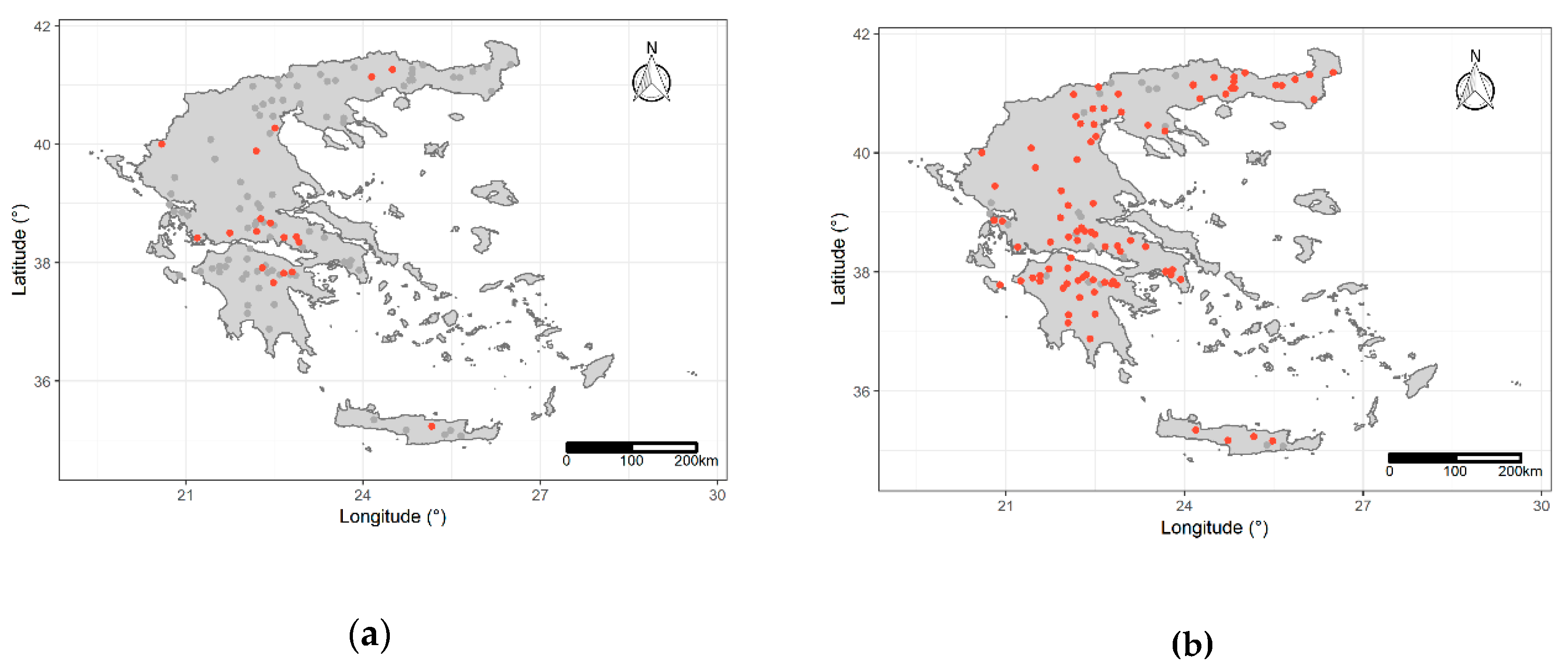
Due to the presence of missing values, a subset of stations was used for the temporal analysis using the criterion that these stations should have 30 years of common time length with coverage at least 45% (18 stations; Figure 3a). The autocorrelation coefficient function and the partial correlation coefficient function were compiled [41,42] to investigate the presence of serial correlation in the annual ED values per station. The test for significance of Kendall’s Tau [43] rank correlation value was first suggested by Mann [44] as a test for trends of a variable versus time and has been used in similar studies about $R$ [45,46,47]. In this analysis and for every selected station the hypothesis that $ED$ does not change over time was tested. In the presence of autocorrelation, a modified version of the test that corrects the p-values was used [48] and the final p-values per station were adjusted using the Benjamini & Hochberg method in order to control the false discovery rate due to multiple statistical testing [49].

2.4. Clustering Analysis

In this part of the analysis, and also due to the presence of missing values, a different subset of stations (84 stations; Figure 3b) was used for the clustering analysis, using the criterion that these stations should have at least 10 values per month with coverage over 45%. The average missing monthly values of $ED$ per station were imputed using linear interpolation, because, in general, clustering algorithms cannot be applied to data with missing values.

Regarding the problem of classification of the stations using the distribution of monthly $ED$ values, initially, and because all the clustering algorithms can return clusters, even if there is no structure in the used data, the Hopkins index, $H$ [50,51], for clustering tendency was applied using the monthly $ED$ values distribution per station. $ED$ is a matrix that was formed using the 84 vectors of the 12 monthly values per station. $H$ can be used to test the null hypothesis of randomly and uniformly distributed data, generated by a Poisson point process and is calculated with:

$$H=\frac{{\sum }_{j=1}^m{u}_j^d}{{\sum }_{j=1}^m{w}_j^d+{\sum }_{j=1}^m{u}_j^d}$$

(6)

where when $X$ is a collection of $n$ data points that have $d$ dimensions, a random sample from $X$ without replacement with members $x_i\left(i=1tom,m\ll n\right)$ is formed and $Y$ is a set of uniformly random data points, also with $d$ dimensions and members $y_j\left(j=1tom\right)$, $u_j$ in turn is the Euclidean distance from $y_j$ to its nearest neighbor in $X$ and $w_j$ is also the Euclidean distance from $x_i$ to its nearest neighbor in $X$. A value of $H$ close to one, indicates that the data are highly clustered, 0.5 indicates randomly distributed data and zero indicates regularly spaced data [52].

The clustering method applied on $ED$ was agglomerative Hierarchical Clustering (HC), because this method does not depend on the prior selection of the number of the clusters, or a random initialization, as for example K-means does [53]. HC requirements are the selection (a) of the dissimilarity measure, for which the Euclidean distance was used:

$$d\left(x_i,y_i\right)=\sqrt{{\displaystyle \sum _{i=1}^{12}}{\left(x_i-y_i\right)}^2}$$

(7)

where $x_i$ and $y_i$ are the monthly $ED$ values from the stations $x$ and $y$; and (b) of the agglomeration method, where the Ward’s minimum variance criterion was selected, an algorithm that minimizes the total within-cluster variance [54], as implemented in the R language [55,56]. At the beginning of the algorithm, the number of the clusters is equal to the number of data points (all clusters contain a single point). At every step, the algorithm finds the pair of clusters that result after merging to the minimum increase of the total within-cluster-variance, which is expressed as the sum of squared differences between the clusters’ centers. Finally, all clusters are combined to one cluster that contains all the data using a hierarchical method.

The result from HC was a tree-based representation of the stations and the method that was applied to determine the optimal number of clusters was a voting scheme of 30 different indices as computed using the R’s language package NbClust [57]. Each one of these metrics determines the relevant number of clusters in data using relative cluster validity.

3. Results and Discussion

3.1. Annual and Monthly Erosivity Density Calculations

Using the pluviograph records from all 108 stations, 100,985 rainfall events were extracted, a subset comprising 27,421 of them were classified as erosive and consequently used in the analysis. Utilizing intensity-duration-frequency curves 87 rainfalls were removed as outliers, because their return period was from 50 to 2284 years (the latter was a single, reported, extreme event in the area of Crete). These return periods caused extreme $E{I}_{30}$ values, up to 12,887 MJ mm/ha/h, that would disproportionately affect the calculations. The first four central moments (mean, standard deviation skewness and kurtosis), and the coefficient of variation are used to describe the annual and monthly values of $ED$ for the 84 stations used in the clustering analysis (

Table 1. Average statistical properties of annual and monthly ED values for the stations used in clustering analysis. SD is an abbreviation for standard deviation and CV for coefficient of variation (the ratio of the standard deviation to the mean).

ED (MJ/ha/h)	Min	Mean	Median	Max	SD	Skew	Kurtosis	CV
January	0.36	1.10	1.08	2.23	0.43	0.38	−0.58	0.39
February	0.52	1.13	1.07	2.40	0.41	0.77	0.10	0.36
March	0.52	1.10	1.05	2.37	0.36	1.06	1.47	0.32
April	0.45	1.07	1.03	2.10	0.32	0.80	0.50	0.30
May	0.37	1.39	1.30	2.64	0.44	0.53	−0.13	0.32
June	0.78	1.76	1.57	3.81	0.68	0.93	0.31	0.38
July	1.08	2.19	1.89	5.45	0.99	1.30	1.23	0.45
August	0.64	1.92	1.84	5.99	0.87	1.80	5.35	0.45
September	0.84	1.75	1.57	3.48	0.67	0.82	−0.25	0.38
October	0.61	1.78	1.66	3.54	0.67	0.90	0.18	0.38
November	0.58	1.68	1.56	3.74	0.65	0.53	−0.21	0.39
December	0.50	1.40	1.38	3.36	0.56	0.62	0.45	0.40
Annual	1.28	2.89	2.75	5.51	1.13	0.60	0.14	0.39

).

A comparison between the results from the energy equation that was used by Panagos and his associates [8] and the one used in the study, showed a systematic underestimation of about 14% percent in the calculations of $E{I}_{30}$ in the previous study. These results are similar to the ones found for Italy, also a Mediterranean country, and from various places worldwide [39], about the variation among RUSLE and RUSLE2.

The computed mean annual value of $ED$ (2.89 MJ/ha/h) is more than two times larger than the value reported for Greece, also by Panagos et al. [8] (1.22 MJ/ha/h). The reason for this difference is that in the previous study the researchers calculated $ED$ as the fraction of $R$ that came from the same pluviograph records (with the missing values issues and the systematic underestimation) and precipitation using a different origin (one-km-global-spatial-resolution monthly values [58]).

The stations’ monthly mean $ED$ values, as well as their annual means are presented in Figure 4. These values, in general, seem to follow the same annual pattern, with higher $ED$ values during summer and autumn. This annual pattern was similar to the one presented by Panagos et al. [8]. A small set of stations appeared to have very large values during summer, and another one had its maximum during autumn.

3.2. Monte Carlo Procedure Results

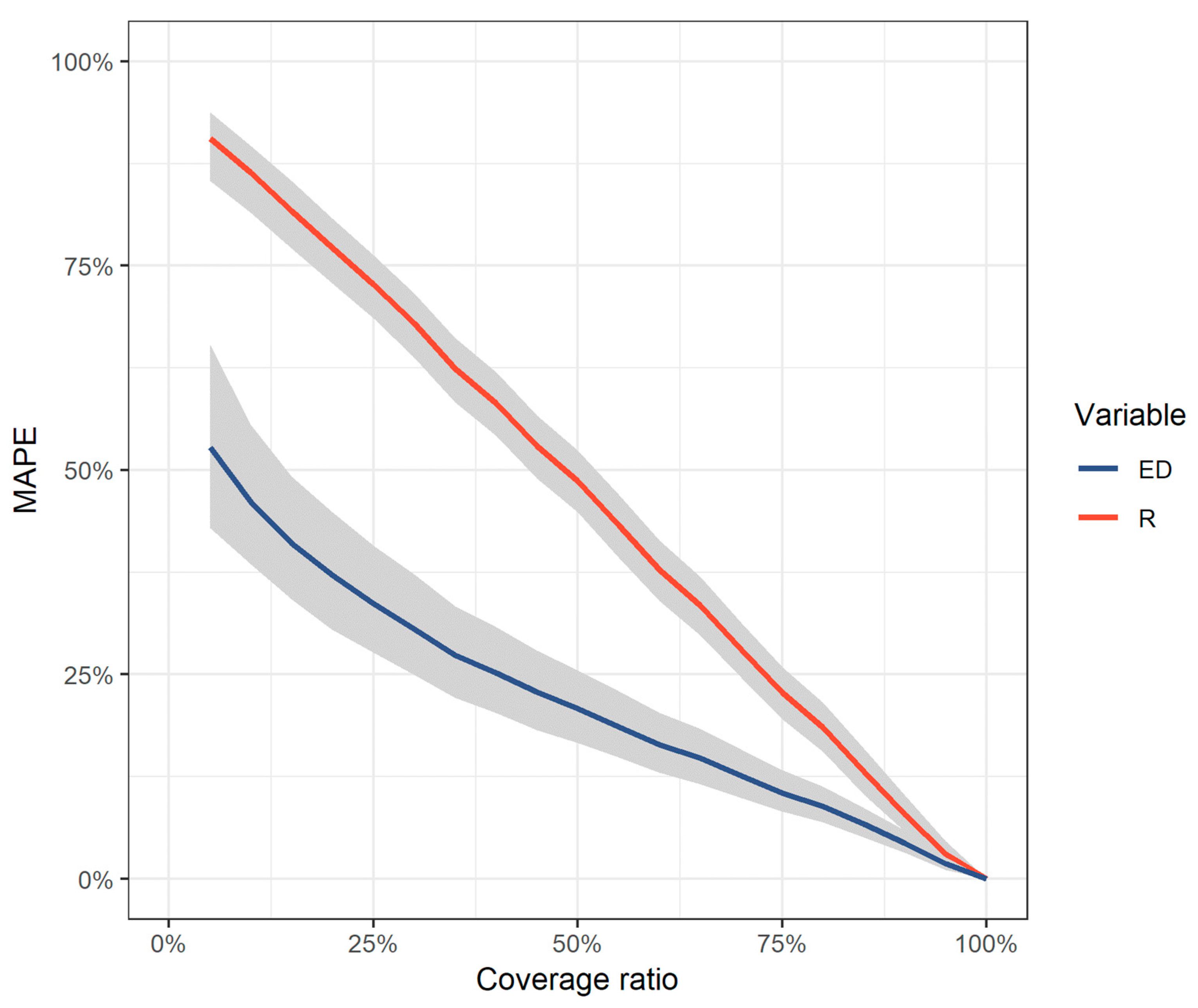
The Monte Carlo procedure results (Figure 5) showed that $ED$ is more robust against the presence of missing precipitation values. Using only 5% of the data, annual $R$ values were underestimated by 85% on average, when the average estimation error of $ED$ values was 50%. $R$ was proportionally underestimated as the missing values ratio increased, while $ED$’s estimation error followed a parabolic curve. In the presence of 50% of the data, R values were underestimated by half, while at the same time the estimation error of $ED$ was 20%.

Even though the impact of missing values to the underestimation of $R$ was expected, it seems that the effect on the calculations of $ED$ is not negligible, as the RUSLE2 developers stated, especially at low data coverage. In any case, it appeared that the use of $ED$ instead of the direct calculations of $R$ should be preferred in any case and especially in the presence of missing values, as is the case with the data from Greece, because it does not introduce systematic errors.

3.3. Erosivity Density Temporal Trends

The findings regarding the $ED$s’ samples autocorrelation coefficient functions and the partial correlation coefficient functions did not reveal any practical meaning of the statistically significant values that were found at specific lags in the time-series of a small number of stations. On account of the previous fact, it was safe to suppose that no stochastic trends existed for the examined time-series.

The Kendall’s Tau rank correlation test results (

Table 2. Location and analysis results for the stations with a common time length during 1965–1996. ID is an abbreviation for the station ID as reported in the Greek National Bank of Hydrological and Meteorological Information, WD for the Greek Water Divisions, Lon for longitude, Lat for latitude, El for elevation, MCV for mean coverage per station, p_adj is the adjusted p-value from the test using the Benjamini & Hochberg method. When a star is marked, it indicates the test results in which the null hypothesis is rejected for a significance level α = 5%.

	ID	Name	WD	Lon (°)	Lat (°)	El (m)	MCV (%)	Tau	padj
1	200003	GRABIA	GR07	22.43	38.67	381	73.4	0.12	0.612
2	200011	LIDORIKI	GR04	22.20	38.53	548	69.2	−0.09	0.612
3	200015	PYRA	GR04	22.27	38.74	1137	74.8	−0.11	0.612
4	200018	AG. TRIADA	GR07	22.92	38.35	400	65.4	0.31	0.081
5	200021	DISTOMO	GR07	22.67	38.43	458	60.3	−0.02	0.919
6	200024	LEIBADIA	GR07	22.87	38.44	176	56	−0.27	0.132
7	200059	BASILIKO	GR05	20.59	40.01	747	75.8	−0.11	0.612
8	200092	ELASSONA	GR08	22.19	39.89	276	71.7	0.02	0.919
9	200135	KALYBIA	GR02	22.30	37.92	822	65.3	0.29	0.123
10	200142	NEMEA	GR02	22.66	37.83	306	63.8	−0.26	0.132
11	200144	SPATHOBOUNI	GR02	22.80	37.85	150	48.1	−0.08	0.612
12	200181	LESINIO	GR04	21.19	38.42	2	59.9	0.45	0.055
13	200190	POROS REG.	GR04	21.75	38.51	182	67.8	−0.11	0.612
14	200243	NEOCHORIO	GR03	22.48	37.67	704	63.2	0.14	0.595
15	200291	A. ARCHANES	GR13	25.16	35.24	392	51.6	0.09	0.612
16	200309	DRAMA	GR11	24.15	41.14	100	69.6	0.10	0.612
17	200311	PARANESTE	GR12	24.50	41.27	122	66.1	−0.46	0.005 *
18	200346	KATERINE	GR09	22.51	40.28	30	64.2	−0.15	0.595

) indicated that for the majority of the stations the null hypothesis that annual $ED$ values didn’t change over time could not be rejected for a significance level α = 5%. Thus, it was reasonable to suppose that these time series were realizations of stationary processes. Of the 18 stations used in this analysis, only the station PARANESTE appeared to have a significant negative temporal trend (Table 2). These results of stationarity did not follow the previously reported trends of the mean annual rain intensities in Greece [19], as $ED$ expresses rainfall intensities. Panagos et al. [8] did not perform a statistical analysis of temporal trends. They presented average values with no trend detection.

3.4. Erosivity Density Spatio-Temporal Clustering

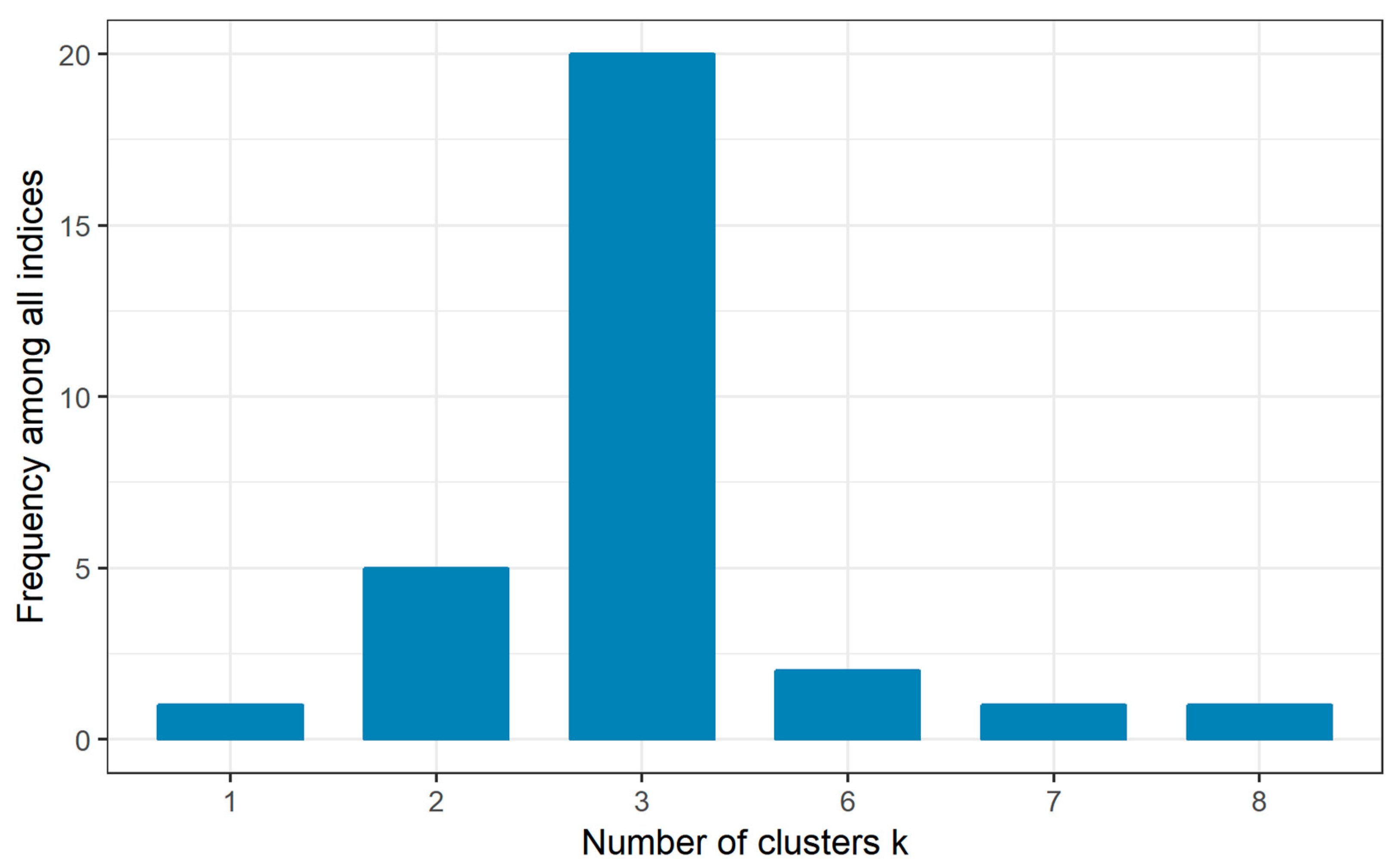
The computed value of the Hopkins index h was 0.70, so the null hypothesis of random data could be safely rejected. This result indicated that there was a physical meaning in the categorization of the stations using their monthly distribution of $ED$ values. After the application of the 30 different indices for the determination of the optimal number of clusters (Figure 6), among all indices 20 proposed three as the best number of clusters and five indices proposed two clusters (

Table 3. Clustering validity indices results. NOC is an abbreviation for Number of Clusters.

Method	KL [60]	CH [61]	Hartigan [62]	CCC [63]	Scott [64]	Marriot [65]	TrCovW [28]	TraceW [28]	Friedman [66]
NOC	3	2	3	2	3	3	3	3	3
Value	2.27	39.70	11.13	12.61	109.02	1.40E+12	568.30	27.72	26.67
Method	Cindex [67]	DB [68]	Silhouette [30]	Duda [69]	PseudoT2 [69]	Beale [70]	Ratkowsky [71]	Ball [72]	PtBiserial [73]
NOC	6	3	3	3	3	7	2	3	3
Value	0.26	1.02	0.39	0.82	14.45	0.54	0.39	57.07	0.75
Method	Frey [74]	McClain [75]	Gamma [76]	Gplus [73]	Tau [73]	Dunn [77]	Hubert [78]	SDindex [79]	Dindex [80]
NOC	1	2	3	3	3	3	6	3	3
Value	NA	0.30	0.89	49.04	787.63	0.30	Graphical	1.97	Graphical
Method	Rubin [66]	Gap [31]	SDbw [81]
NOC	3	2	8
Value	−1.06	−0.36	0.34

). According to the majority rule it seemed that three was the suitable number of clusters in the dataset.

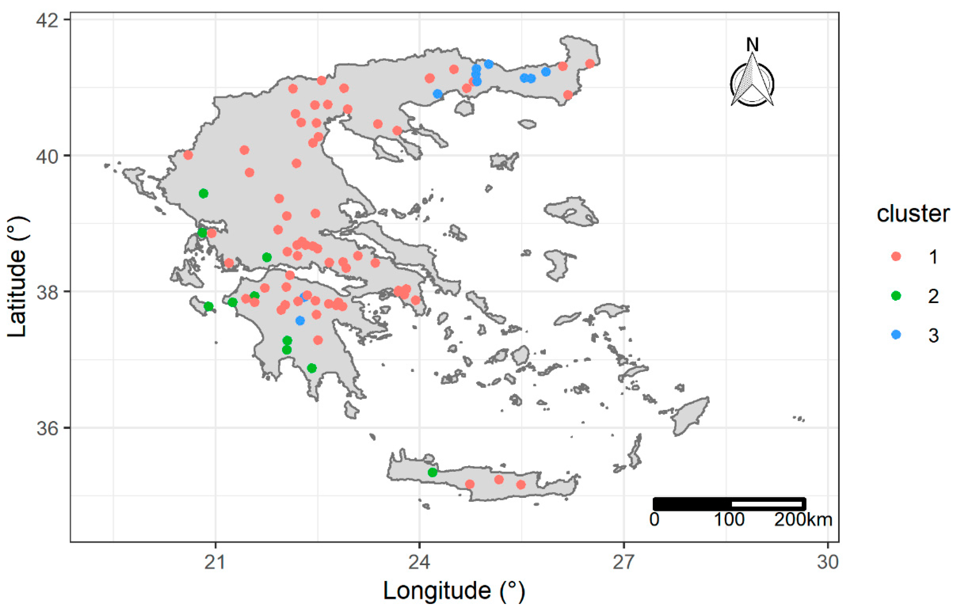
The first four central moments (mean, standard deviation skewness and kurtosis), and the coefficient of variation were used to describe the mean monthly $ED$ of the three clusters (

Table 4. Statistical properties of the mean monthly ED values of the clusters (centers of the clusters). SD is an abbreviation for standard deviation and CV for coefficient of variation.

ED (MJ/ha/h)	Min	Mean	Median	Max	SD	Skew	Kurtosis	CV
Cluster 1	0.97	1.34	1.35	1.89	0.31	0.18	−1.44	0.23
Cluster 2	1.52	2.06	1.86	3.09	0.55	0.67	−1.21	0.27
Cluster 3	1.00	2.09	2.00	4.01	0.89	0.79	−0.48	0.43

). These three clusters are presented in Figure 7 as a map.

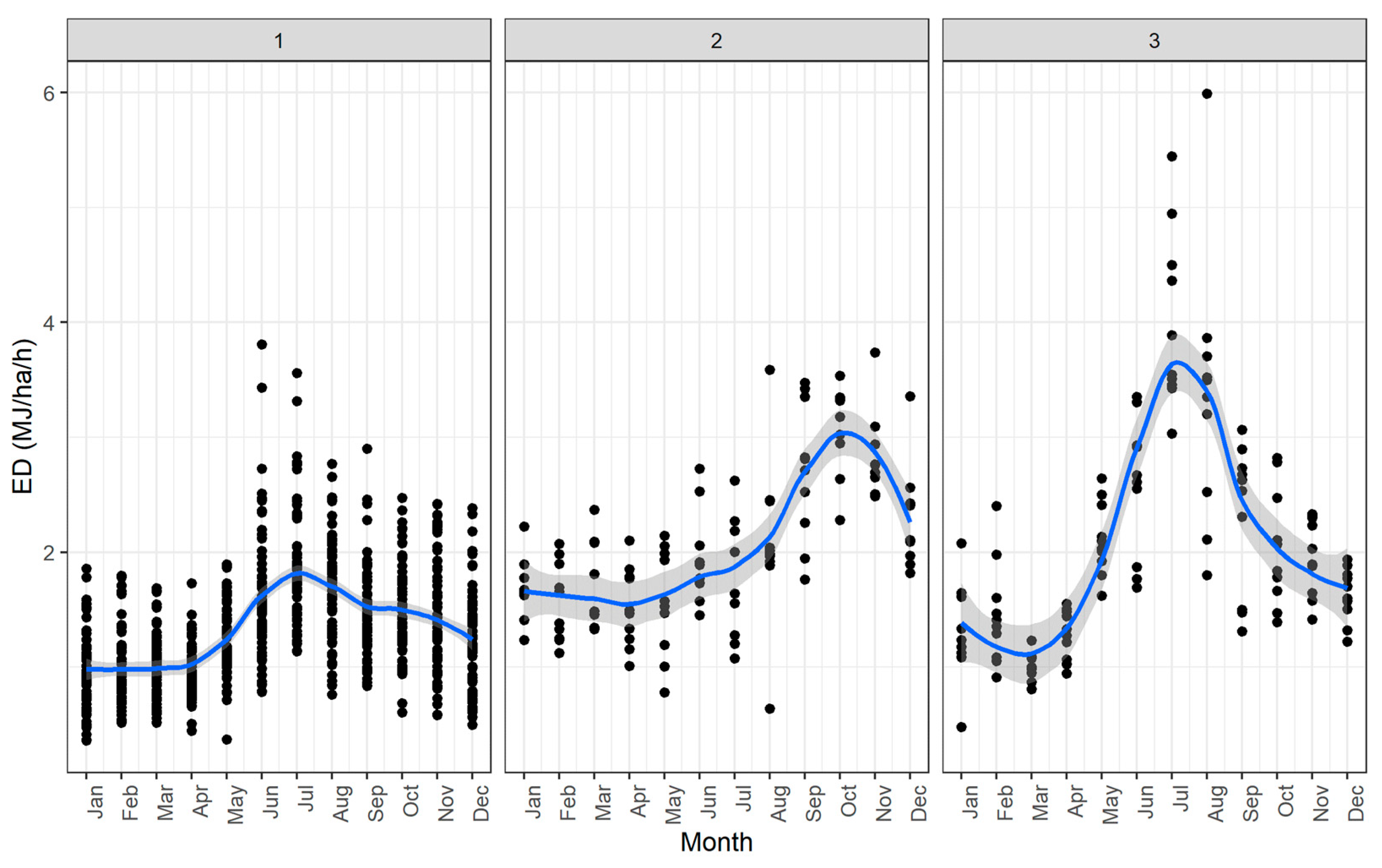
In Figure 8, Local Polynomial Regression Fitting (LOESS [82]) was used as a non-parametric method to produce smooth curves through the monthly $ED$ values of the stations for each of the three clusters. In that method, the fitting is done locally for a given point x using all the points in the neighborhood of x and the distances of these points from x as weights.

The emerged three patterns followed different spatial and temporal distributions. Most of the stations located in the eastern part of Greece, which is drier (rain-shadow) had their maximum of $ED$ values in July and belong to the cluster number one. Cluster number two was located in the western and wetter part of the country (rain-side), where $ED$ values had their maximum in October. A third area that consisted a) mostly of stations located in the north-east part of Greece and b) of two stations at the center of Peloponnesus at south Greece, also had their maximum in the summer. Both clusters two and three had larger $ED$ values and variance on average than the first cluster. Panagos et al. [8], did not identify these areas but reported that there is “high spatial and temporal variability of $ED$”.

4. Conclusions

Summarizing, the main conclusions of our study are:

• Incomplete pluviograph data can be used to compute $ED$ and achieve acceptable accuracy on the estimation of $R$.
• Stationarity of $ED$ was found for the majority of the selected stations in Greece.
• Three clusters of stations define areas in Greece with different temporal patterns of $ED$.
• Only the stations that are located in the rainy part of western Greece have $ED$ values that follow the seasonal cycle of precipitation that is common for the country.

The comparative assessment of the impact of missing data on both $R$ and $ED$ using a numerical scheme and data coming from a national database (Greece) was one of the results of this paper. The Monte-Carlo simulation showed that it is suggested to compute $ED$ for the assessment of erosivity instead of a direct computation of $R$ in the presence of incomplete data. A small fraction of pluviograph data can be used to compute $ED$ and achieve acceptable accuracy during the estimation of $R$ in conjunction with precipitation data consisting of coarser values such as daily or monthly, which are available on a larger spatial and temporal extent, not only in Greece, but worldwide.

In this paper, contrary to a previous study on the country, (a) the methodology that is used in RUSLE2 was applied, (b) monthly and annual $ED$ values were calculated for 108 stations without the presence of outliers and (c) corrections were made due to the use of 30-minutes-fixed- time-interval data instead of breakpoint rainfall data. As a result, the mean value of $ED$ calculated here is more than two times larger than the value previously reported. Consequently, and due to the presence of a large proportion of missing values, the previously reported $R$ values for the country were also underestimated. Furthermore, stationarity of annual values of $ED$ was found for the majority of the stations that share a time length of 30 years, in contrast to the reported precipitation and rainfall intensity trends for the same time period in Greece.

An unsupervised analysis that has not been applied for the specific problem in the bibliography was used and identified three clusters of stations in Greece that define areas with different temporal patterns of monthly $ED$ values, in other words areas with different seasonal distributions of intense and erosive rainfalls. These patterns can also be used to estimate $R$ values in Greece, using coarser precipitation data. Only the stations that are located in the rainy part of western Greece have $ED$ values that follow the same, common, seasonal cycle of precipitation in the country, with their maximum values occurring during autumn. The stations located to the eastern part have their maximum values during summer and an area that is located to the north-east part of Greece emerged, with higher variability and absolute values of $ED$ than the rest.

References

- Jacob, D.; Petersen, J.; Eggert, B.; Alias, A.; Christensen, O.B.; Bouwer, L.M.; Braun, A.; Colette, A.; Déqué, M.; Georgievski, G.; et al. EURO-CORDEX: New high-resolution climate change projections for European impact research. Reg. Environ. Chang. 2014, 14, 563–578. [Google Scholar] [CrossRef]
- Nearing, M.; Pruski, F.; O’neal, M. Expected climate change impacts on soil erosion rates: A review. J. Soil Water Conserv. 2004, 59, 43–50. [Google Scholar]
- Hellenic Republic. Acceptance of the Greek National Action Plan against Desertification; Joint Ministerial Decision: Athens, Greece, 2001. [Google Scholar]
- Kosmas, C.; Danalatos, N.; Kosma, D.; Kosmopoulou, P. Greece. In Soil Erosion in Europe; John Wiley & Sons: Hoboken, NJ, USA, 2006; pp. 279–288. ISBN 978-0-470-85920-9. [Google Scholar]
- Wischmeier, W.H.; Smith, D.D. Predicting Rainfall Erosion Losses—A Guide to Conservation Planning; USDA, Agriculture Handbook No. 537; Government Printing Office: Washington, DC, USA, 1978.
- Renard, K.G.; Foster, G.R.; Weesies, G.A.; McCool, D.K.; Yoder, D.C. Predicting Soil Erosion by Water: A Guide to Conservation Planning with the Revised Universal Soil Loss Equation (RUSLE); Department of Agriculture: Washington, DC, USA, 1997; Volume 703.
- USDA-ARS. Science Documentation: Revised Universal Soil Loss Equation, Version 2 (RUSLE 2); USDA-Agricultural Research Service: Washington, DC, USA, 2013.
- Panagos, P.; Ballabio, C.; Borrelli, P.; Meusburger, K. Spatio-temporal analysis of rainfall erosivity and erosivity density in Greece. Catena 2016, 137, 161–172. [Google Scholar] [CrossRef] [Green Version]
- Vantas, K. Determination of Rainfall Erosivity in the Framework of Data Science Using Machine Learning and Geostatistics Methods. Ph.D. Thesis, Aristotle University of Thessaloniki, Thessaloniki, Greece, 2017. [Google Scholar]
- Vantas, K.; Sidiropoulos, E. Imputation of erosivity values under incomplete rainfall data by machine learning methods. Eur. Water 2017, 57, 193–199. [Google Scholar]
- Brown, L.C.; Foster, G.R. Storm erosivity using idealized intensity distributions. Trans. ASAE 1987, 30, 379–386. [Google Scholar] [CrossRef]
- Nearing, M.A.; Yin, S.; Borrelli, P.; Polyakov, V.O. Rainfall erosivity: An historical review. Catena 2017, 157, 357–362. [Google Scholar] [CrossRef]
- Hollinger, S.E.; Angel, J.R.; Palecki, M.A. Spatial Distribution, Variation, and Trends in Storm Precipitation Characteristics Associated with Soil Erosion in the United States; Illinois State Water Survey Atmospheric Environment Section: Champaign, IL, USA, 2002. [Google Scholar]
- Feidas, H.; Noulopoulou, C.; Makrogiannis, T.; Bora-Senta, E. Trend analysis of precipitation time series in Greece and their relationship with circulation using surface and satellite data: 1955–2001. Theor. Appl. Climatol. 2007, 87, 155–177. [Google Scholar] [CrossRef]
- Bartzokas, A.; Lolis, C.J.; Metaxas, D.A. A study on the intra-annual variation and the spatial distribution of precipitation amount and duration over Greece on a 10 day basis. Int. J. Climatol. J. R. Meteorol. Soc. 2003, 23, 207–222. [Google Scholar] [CrossRef] [Green Version]
- Xoplaki, E.; Luterbacher, J.; Burkard, R.; Patrikas, I.; Maheras, P. Connection between the large-scale 500 hPa geopotential height fields and precipitation over Greece during wintertime. Clim. Res. 2000, 14, 129–146. [Google Scholar] [CrossRef]
- Tolika, K.; Maheras, P. Spatial and temporal characteristics of wet spells in Greece. Theor. Appl. Climatol. 2005, 81, 71–85. [Google Scholar] [CrossRef]
- Maheras, P.; Tolika, K.; Anagnostopoulou, C.; Vafiadis, M.; Patrikas, I.; Flocas, H. On the relationships between circulation types and changes in rainfall variability in Greece. Int. J. Climatol. J. R. Meteorol. Soc. 2004, 24, 1695–1712. [Google Scholar] [CrossRef] [Green Version]
- Kambezidis, H.D.; Larissi, I.K.; Nastos, P.T.; Paliatsos, A.G. Spatial variability and trends of the rain intensity over Greece. Adv. Geosci. 2010, 26, 65–69. [Google Scholar] [CrossRef] [Green Version]
- Markonis, Y.; Batelis, S.C.; Dimakos, Y.; Moschou, E.; Koutsoyiannis, D. Temporal and spatial variability of rainfall over Greece. Theor. Appl. Climatol. 2017, 130, 217–232. [Google Scholar] [CrossRef]
- Hatzianastassiou, N.; Katsoulis, B.; Pnevmatikos, J.; Antakis, V. Spatial and temporal variation of precipitation in Greece and surrounding regions based on global precipitation climatology project data. J. Clim. 2008, 21, 1349–1370. [Google Scholar] [CrossRef]
- Abu-Mostafa, Y.S.; Magdon-Ismail, M.; Lin, H.-T. Learning from Data; AMLBook: New York, NY, USA, 2012. [Google Scholar]
- Sheikholeslami, G.; Chatterjee, S.; Zhang, A. Wavecluster: A multi-resolution clustering approach for very large spatial databases. In Proceedings of the VLDB Conference, New York, NY, USA, 24–27 August 1998; Volume 98, pp. 428–439. [Google Scholar]
- Hartigan, J.A.; Wong, M.A. Algorithm AS 136: A k-means clustering algorithm. J. R. Stat. Soc. Ser. C (Appl. Stat.) 1979, 28, 100–108. [Google Scholar] [CrossRef]
- MacQueen, J. Some methods for classification and analysis of multivariate observations. In Proceedings of the Fifth Berkeley Symposium on Mathematical Statistics and Probability; University of California Press: Berkley, CA, USA; Los Angeles, CA, USA, 1967; Volume 1, pp. 281–297. [Google Scholar]
- Ward, J.H., Jr. Hierarchical grouping to optimize an objective function. J. Am. Stat. Assoc. 1963, 58, 236–244. [Google Scholar] [CrossRef]
- Theodoridis, S.; Koutroumbas, K. Pattern Recognition; Academic Press: Burlington, MA, USA, 2008; ISBN 978-1-59749-272-0. [Google Scholar]
- Milligan, G.W.; Cooper, M.C. An examination of procedures for determining the number of clusters in a data set. Psychometrika 1985, 50, 159–179. [Google Scholar] [CrossRef]
- Charrad, M.; Ghazzali, N.; Boiteau, V.; Niknafs, A. NbClust: An R package for determining the relevant number of clusters in a data set. J. Stat. Softw. 2014, 61, 1–36. [Google Scholar] [CrossRef]
- Rousseeuw, P.J. Silhouettes: A graphical aid to the interpretation and validation of cluster analysis. J. Comput. Appl. Math. 1987, 20, 53–65. [Google Scholar] [CrossRef] [Green Version]
- Tibshirani, R.; Walther, G.; Hastie, T. Estimating the number of clusters in a data set via the gap statistic. J. R. Stat. Soc. Ser. B (Stat. Methodol.) 2001, 63, 411–423. [Google Scholar] [CrossRef] [Green Version]
- Vantas, K.; Sidiropoulos, E.; Loukas, A. Temporal and elevation trend detection of rainfall erosivity density in Greece. Proceedings 2019, 7, 10. [Google Scholar] [CrossRef]
- Vantas, K. hydroscoper: R interface to the Greek national data bank for hydrological and meteorological information. J. Open Source Softw. 2018, 3, 625. [Google Scholar] [CrossRef]
- Weiss, L.L. Ratio of true to fixed-interval maximum rainfall. J. Hydraul. Div. 1964, 90, 77–82. [Google Scholar]
- Hershfield, D.M. Rainfall Frequency Atlas of the United States; U.S. Department of Commerce, Weather Bureau: Washington, DC, USA, 1961; Volume 40.
- Van Montfort, M.A.J. Concomitants of the Hershfield factor. J. Hydrol. 1997, 194, 357–365. [Google Scholar] [CrossRef]
- Yin, S.; Xie, Y.; Nearing, M.A.; Wang, C. Estimation of rainfall erosivity using 5-to 60-minute fixed-interval rainfall data from China. Catena 2007, 70, 306–312. [Google Scholar] [CrossRef]
- McGregor, K.C.; Bingner, R.L.; Bowie, A.J.; Foster, G.R. Erosivity index values for northern Mississippi. Trans. ASAE 1995, 38, 1039–1047. [Google Scholar] [CrossRef]
- Yin, S.; Nearing, M.A.; Borrelli, P.; Xue, X. Rainfall erosivity: An overview of methodologies and applications. Vadose Zone J. 2017, 16. [Google Scholar] [CrossRef]
- Hellenic Republic. Implementation of Directive 2007/60 EC—Development of Rainfall Curves in Greece; Special Water Secretariat: Athens, Greece, 2016. [Google Scholar]
- Venables, W.N.; Ripley, B.D. Modern Applied Statistics with S, 4th ed.; Springer: New York, NY, USA, 2002. [Google Scholar]
- Box, G.E.; Jenkins, G.M.; Reinsel, G.C.; Ljung, G.M. Time Series Analysis: Forecasting and Control; John Wiley & Sons: Hoboken, NJ, USA, 2015. [Google Scholar]
- Kendall, M.G. Rank Correlation Methods; Rank Correlation Methods; Griffin: Oxford, UK, 1948. [Google Scholar]
- Mann, H.B. Nonparametric tests against trend. Econ. J. Econ. Soc. 1945, 1, 245–259. [Google Scholar] [CrossRef]
- Petek, M.; Mikoš, M.; Bezak, N. Rainfall erosivity in Slovenia: Sensitivity estimation and trend detection. Environ. Res. 2018, 167, 528–535. [Google Scholar] [CrossRef]
- Fiener, P.; Neuhaus, P.; Botschek, J. Long-term trends in rainfall erosivity–analysis of high resolution precipitation time series (1937–2007) from Western Germany. Agric. For. Meteorol. 2013, 171, 115–123. [Google Scholar] [CrossRef]
- Meusburger, K.; Steel, A.; Panagos, P.; Montanarella, L.; Alewell, C. Spatial and temporal variability of rainfall erosivity factor for Switzerland. Hydrol. Earth Syst. Sci. 2012, 16, 167–177. [Google Scholar] [CrossRef] [Green Version]
- Hamed, K.H.; Rao, A.R. A modified Mann-Kendall trend test for autocorrelated data. J. Hydrol. 1998, 204, 182–196. [Google Scholar] [CrossRef]
- Benjamini, Y.; Hochberg, Y. Controlling the false discovery rate: A practical and powerful approach to multiple testing. J. R. Stat. Soc. Ser. B (Methodol.) 1995, 57, 289–300. [Google Scholar] [CrossRef]
- Lawson, R.G.; Jurs, P.C. New index for clustering tendency and its application to chemical problems. J. Chem. Inf. Comput. Sci. 1990, 30, 36–41. [Google Scholar] [CrossRef]
- Hopkins, B.; Skellam, J.G. A new method for determining the type of distribution of plant individuals. Ann. Bot. 1954, 18, 213–227. [Google Scholar] [CrossRef]
- Theodoridis, S.; Koutroumbas, K. Pattern Recognition, 4th ed.; Elsevier Academic Press: Amsterdam, The Netherlands, 2009; ISBN 978-1-59749-272-0. [Google Scholar]
- Friedman, J.; Hastie, T.; Tibshirani, R. The Elements of Statistical Learning; Springer Series in Statistics; Springer: New York, NY, USA, 2001; Volume 1. [Google Scholar]
- Husson, F.; Lê, S.; Pagès, J. Exploratory Multivariate Analysis by Example Using R, 2nd ed.; Chapman and Hall/CRC: New York, NY, USA, 2017; ISBN 978-0-429-22543-7. [Google Scholar]
- R Core Team R: A Language and Environment for Statistical Computing; R Foundation for Statistical Computing: Vienna, Austria, 2019.
- Murtagh, F.; Legendre, P. Ward’s hierarchical agglomerative clustering method: Which algorithms implement Ward’s criterion? J. Classif. 2014, 31, 274–295. [Google Scholar] [CrossRef]
- Charrad, M.; Ghazzali, N.; Boiteau, V.; Niknafs, A. NbClust: Determining the Best Number of Clusters in a Data Set. 2015. Available online: https://cran.r-project.org/web/packages/NbClust/index.html (accessed on 17 May 2019).
- Hijmans, R.J.; Cameron, S.E.; Parra, J.L.; Jones, P.G.; Jarvis, A. Very high resolution interpolated climate surfaces for global land areas. Int. J. Climatol. 2005, 25, 1965–1978. [Google Scholar] [CrossRef] [Green Version]
- Shyu, W.M.; Grosse, E.; Cleveland, W.S. Local regression models. In Statistical Models in S; Routledge: London, UK, 2017; pp. 309–376. [Google Scholar]
- Krzanowski, W.J.; Lai, Y.T. A criterion for determining the number of groups in a data set using sum-of-squares clustering. Biometrics 1988, 44, 23–34. [Google Scholar] [CrossRef]
- Caliński, T.; Harabasz, J. A dendrite method for cluster analysis. Commun. Stat.-Theory Methods 1974, 3, 1–27. [Google Scholar] [CrossRef]
- Hartigan, J.A. Clustering Algorithms; Wiley Series in Probability and Mathematical Statistics; Wiley: New York, NY, USA, 1975. [Google Scholar]
- Sarle, W.S. SAS technical report A-108, cubic clustering criterion. Cary NC SAS Inst. Inc. 1983, 56. [Google Scholar]
- Scott, A.J.; Symons, M.J. Clustering methods based on likelihood ratio criteria. Biometrics 1971, 27, 387–397. [Google Scholar] [CrossRef]
- Marriott, F.H.C. Practical problems in a method of cluster analysis. Biometrics 1971, 27, 501–514. [Google Scholar] [CrossRef]
- Friedman, H.P.; Rubin, J. On some invariant criteria for grouping data. J. Am. Stat. Assoc. 1967, 62, 1159–1178. [Google Scholar] [CrossRef]
- Hubert, L.J.; Levin, J.R. A general statistical framework for assessing categorical clustering in free recall. Psychol. Bull. 1976, 83, 1072–1080. [Google Scholar] [CrossRef]
- Davies, D.L.; Bouldin, D.W. A Cluster separation measure. IEEE Trans. Pattern Anal. Mach. Intell. 1979, PAMI-1, 224–227. [Google Scholar] [CrossRef]
- Duda, R.O.; Hart, P.E.; Stork, D.G. Pattern Classification and Scene Analysis; Wiley: New York, NY, USA, 1973; Volume 3. [Google Scholar]
- Beale, E.M.L. Cluster Analysis; Scientific Control Systems Limited: London, UK, 1969. [Google Scholar]
- Ratkowsky, D.A.; Lance, G.N. Criterion for determining the number of groups in a classification. Aust. Comput. J. 1978, 10, 115–117. [Google Scholar]
- Ball, G.H.; Hall, D.J. ISODATA, a Novel Method of Data Analysis and Pattern Classification; Stanford Research Inst.: Menlo Park, CA, USA, 1965. [Google Scholar]
- Milligan, G.W. A monte carlo study of thirty internal criterion measures for cluster analysis. Psychometrika 1981, 46, 187–199. [Google Scholar] [CrossRef]
- Frey, T.; van Groenewoud, H. A cluster analysis of the D2 matrix of white spruce stands in Saskatchewan based on the maximum-minimum principle. J. Ecol. 1972, 60, 873–886. [Google Scholar] [CrossRef]
- McClain, J.O.; Rao, V.R. Clustisz: A program to test for the quality of clustering of a set of objects. JMR J. Mark. Res. (pre-1986) 1975, 12, 456. [Google Scholar]
- Baker, F.B.; Hubert, L.J. Measuring the power of hierarchical cluster analysis. J. Am. Stat. Assoc. 1975, 70, 31–38. [Google Scholar] [CrossRef]
- Dunn, J.C. Well-separated clusters and optimal fuzzy partitions. J. Cybern. 1974, 4, 95–104. [Google Scholar] [CrossRef]
- Hubert, L.; Arabie, P. Comparing partitions. J. Classif. 1985, 2, 193–218. [Google Scholar] [CrossRef]
- Halkidi, M.; Vazirgiannis, M.; Batistakis, Y. Quality scheme assessment in the clustering process. In Proceedings of the Principles of Data Mining and Knowledge Discovery; Zighed, D.A., Komorowski, J., Żytkow, J., Eds.; Springer: Berlin, Germany, 2000; pp. 265–276. [Google Scholar]
- Lebart, L.; Morineau, A.; Piron, M. Statistique Exploratoire Multidimensionnelle; Dunod: Paris, France, 2000. [Google Scholar]
- Halkidi, M.; Vazirgiannis, M. Clustering validity assessment: Finding the optimal partitioning of a data set. In Proceedings of the 2001 IEEE International Conference on Data Mining, San Jose, CA, USA, 29 November–2 December 2001; pp. 187–194. [Google Scholar]
- Cleveland, W.S.; Grosse, E.; Shyu, W.M. Local regression models. In Statistical Models in S; Chapman & Hall: New York, NY, USA, 1992; pp. 309–376. [Google Scholar]
- Vantas, K. Hyetor: R Package to Analyze Fixed Interval Precipitation Time Series. 2019. Available online: https://github.com/kvantas/hyetor (accessed on 17 May 2019).
- Wickham, H. Ggplot2: Elegant Graphics for Data Analysis; Springer: New York, NY, USA, 2009; ISBN 978-0-387-98140-6. [Google Scholar]
Figure 1.
Flowchart of the applied methodology.
Figure 2.
Station locations in Greece used in the analysis obtained from the Greek National Bank of Hydrological and Meteorological Information.
Figure 3.
In these figures, the different subsets of stations used in the analysis are presented with red color: (a) Stations used for the temporal trend analysis; (b) Stations used for the clustering analysis.
Figure 4.
The grey lines represent the average monthly ED of all the stations used in clustering analysis. Some of these lines have no values for some months due to missing values. The red line symbolizes the mean annual ED values coming from all the stations, after smoothing by means of Local Polynomial Regression Fitting [59], as a non-parametric method to present smooth curves between the plotted variables.
Figure 5.
Results from the Monte Carlo procedure that was employed for the assessment of missing values ratio to the computation of annual and values. Grey bands symbolize the interquartile range (i.e., the 25th and 75th percentiles of the errors) per variable. Lower values of MAPE mean smaller error.
Figure 6.
The above plot presents the frequency among all 30 indices used for the determination of the optimal number of clusters.
Figure 7.
Stations’ clusters using monthly distribution of values.
Figure 8.
Monthly distribution values from the emerged clusters. Black dots symbolize the monthly values per station. The blue lines are the LOESS lines that are fitted to the data per cluster. The grey areas represent the standard error of LOESS.