A Study on Climate-Driven Flash Flood Risks in the Boise River Watershed, Idaho


1
Department of Soil and Water Systems, University of Idaho, 322E. Front ST, Boise, ID 83702, USA
2
Texas A&M AgriLife Research (Texas A&M University System), P.O. Box 1658, Vernon, TX 76384, USA
*
Author to whom correspondence should be addressed.
Water 2019, 11(5), 1039; https://doi.org/10.3390/w11051039
Submission received: 15 March 2019
/
Revised: 13 May 2019
/
Accepted: 14 May 2019
/
Published: 18 May 2019
(This article belongs to the Special Issue Extreme Floods and Droughts under Future Climate Scenarios)
Abstract
:We conducted a study on climate-driven flash flood risk in the Boise River Watershed using flood frequency analysis and climate-driven hydrological simulations over the next few decades. Three different distribution families, including the Gumbel Extreme Value Type I (GEV), the 3-parameter log-normal (LN3) and log-Pearson type III (LP3) are used to explore the likelihood of potential flash flood based on the 3-day running total streamflow sequences (3D flows). Climate-driven ensemble streamflows are also generated to evaluate how future climate variability affects local hydrology associated with potential flash flood risks. The result indicates that future climate change and variability may contribute to potential flash floods in the study area, but incorporating embedded-uncertainties inherited from climate models into water resource planning would be still challenging because grand investments are necessary to mitigate such risks within institutional and community consensus. Nonetheless, this study will provide useful insights for water managers to plan out sustainable water resources management under an uncertain and changing climate.
1. Introduction
Climate variability and change continues to increase the risk and frequency of floods for inland communities in the United States (US) [1,2,3,4]. Floods in 2017 alone claimed more than 3 billion dollars in property damages and crop losses [5]. As global warming shifts rainfall patters, more frequent heavy rain is likely contributing to flash floods at the urban-rural interface, such as the Boise River Watershed (BRW) [6]. In general, snowmelt-streamflow dominates high volume in many western watersheds during spring and summer [7,8]. Thus, heavy snowfall and accumulation in winter can elevate potential risks of flash flooding during snow-melting season. Over the last few years, this consequence of heavy snowfall often affects streamflow augmentation in the Boise River so that the second highest inflows to reservoirs upstream is recorded in water year 2017 (October 2016–September 2017) [9]. Such a high-volume water condition began increasing management concerns for reservoir operators and homeowners who live in the flood plain.
Recent studies show that the global climate cycle will create and intensify more severe frequent floods in many regions, resulting in threats to the reliability and resiliency of water resources infrastructure [10,11]. Many previous studies have investigated long-term hydrologic variability associated with climate change [12,13,14,15]. The general circulation models (GCMs) are commonly used to characterize local hydrologic conditions induced by climate variability and change over the next few decades. For instance, because of the timing change of snowfall and snowmelt in the western states, regional water resources management is increasingly facing additional challenges; thus, heavy snowfall increases potential risks of flash flood in the snow-dominated watershed. Floods may also intensify in many regions where total precipitation is even projected to decline due to climate uncertainties [14,15,16]. Based on the evidence of a larger proportion of snowmelt-driven streamflow volume during springtime leveraged by temperature increase, potential impacts of climate change on streamflow in the western states are likely increasing [12,17].
Many previous studies, however, focused on hydrologic consequence of climate change scenarios using statistical downscaling and bias correction processes [13,18,19]. Thus, given the dominantly linear response of the GCMs, future perturbations of hydrologic cycles induced by climate change were investigated to characterize climate-induced hydrological impacts at the regional scales. Relatively little study has been done to explore the risk of potential flash floods associated with climate variability using frequency analysis [20].
In this study, therefore, we investigate how future climate variability can characterize potential flash flood risks in the Boise River Watershed. Using both flood frequency analysis and future ensemble streamflow generations with climate inputs, potential flash flood events are analyzed. We anticipate that the result from this study will provide useful insights for local water managers to plan out future flood mitigation strategies in a changing global environment.
2. Study Area
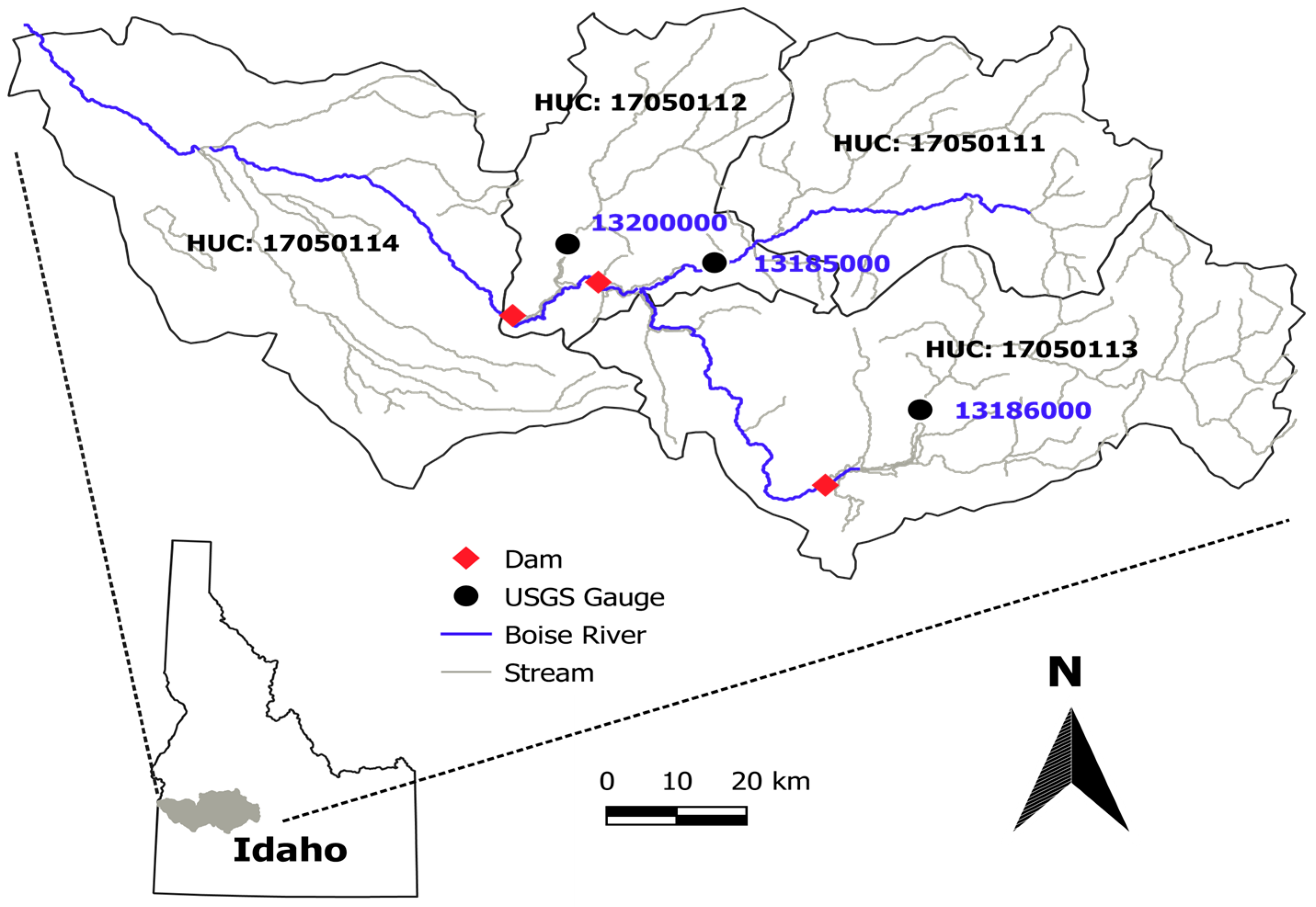
The Boise River Watershed (BRW) is selected as the study area (Figure 1). As a tributary of the Snake River system, the BRW plays a key role of providing water to Boise metropolitan areas, including Boise, Nampa, Meridian, and Caldwell. The drainage area of the basin is about 10,619 km2 with a mainstream length of 164 km stretch and flows into the Snake River near Parma. More than 40% of Idaho residents live in this basin and 60% of people of that are residing around the floodplain [21]. The main physical and geographic characteristic of the BRW is a greater proportion of precipitation falling at higher elevations. It becomes the cause of predictably high flows due to the snow melting process so that the localized flood event is often observed during late spring and early summer.
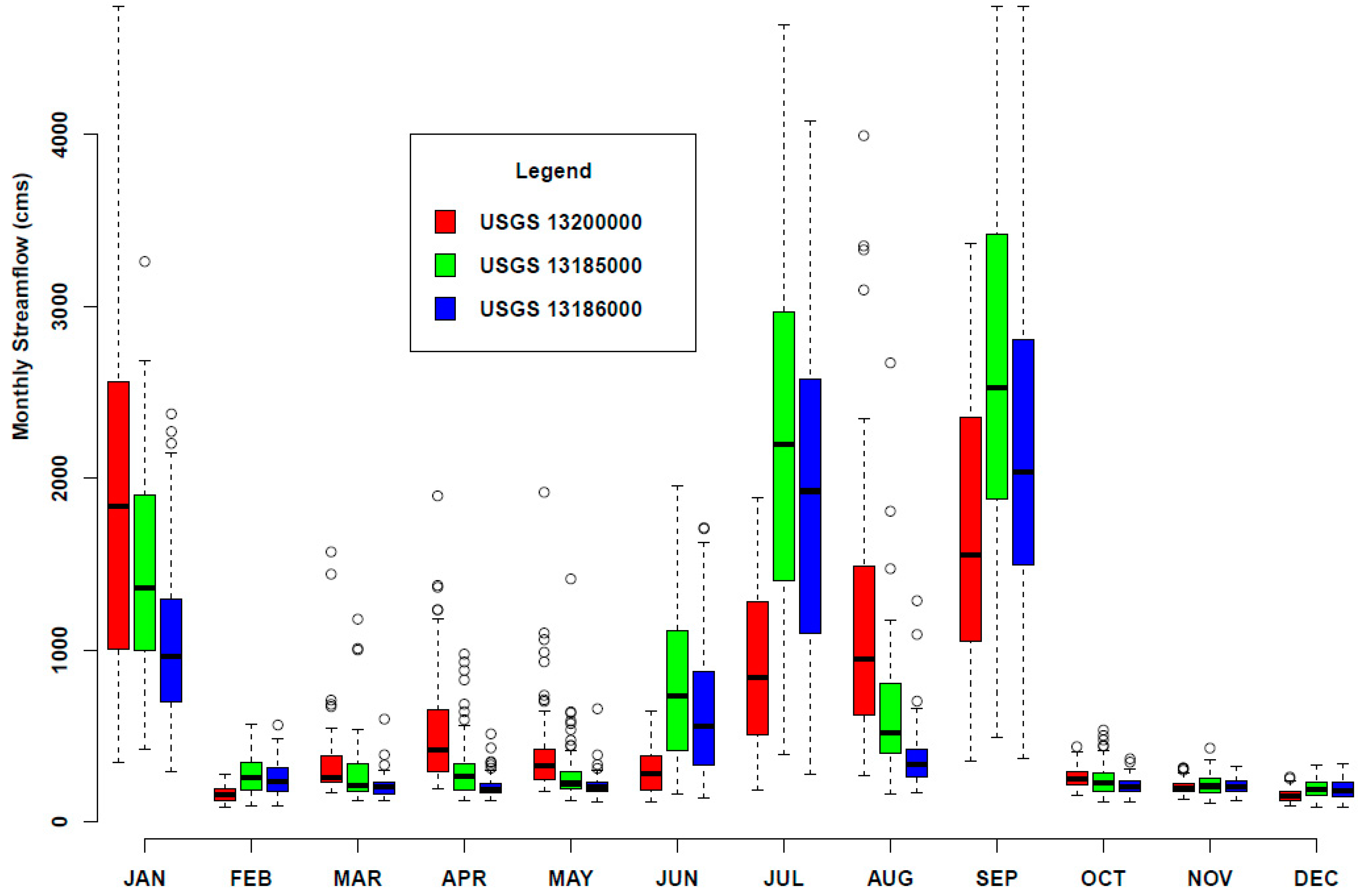
The recent flash flood induced by heavy snowfall 2017 further highlights a research proposal to increase water storage capacity of the Boise River system by raising small-portion elevation of the existing dams, including Lucky Peak, Arrowrock and Anderson Ranch. The Bureau of Reclamation is currently conducting the feasibility study of the dams under the December 2016 Federal Water Infrastructure Improvements for the Nation Act, which may also authorize funding for construction of projects by 1 January 2021 [22]. Additional water capacity in the BRW (if this project is complete) will provide more flexibility for water managers to mitigate impacts driven by climate-induced hydro extremes (flood and drought). Seasonal streamflow for three stations managed by United States Geological Survey (USGS), including USGS: 13200000 (OBS1), 13185000 (OBS2) and 13186000 (OBS3) are observed. As shown in Figure 2, the seasonal trends at these stations are distinct in the sense that snow-melting streamflows are dominant during summer, while rainfalls in later fall is also contributing to streamflow before major snowfall starts.
3. Methodology
3.1. Flash Flood Frequency
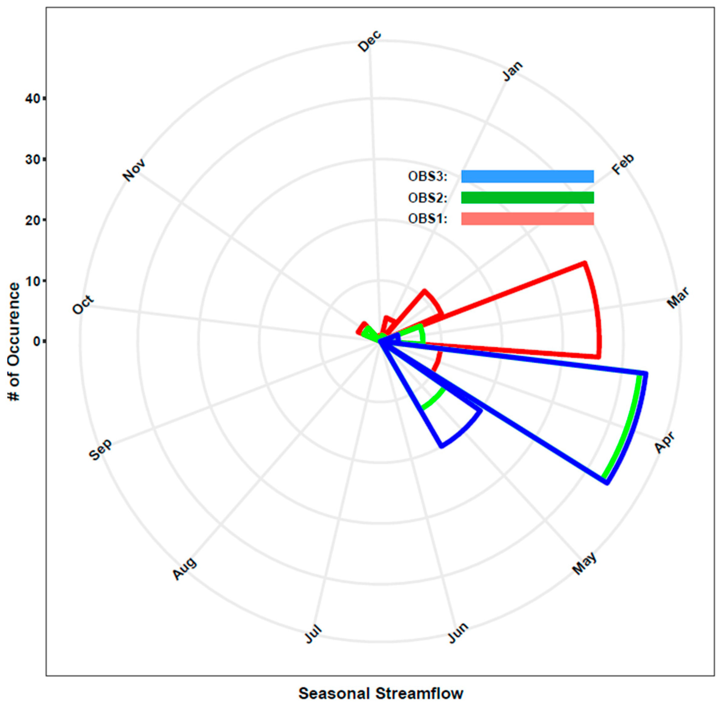
For flood frequency analysis, the magnitudes of a single hydro variable, such as annual maximum flood peak is widely used in hydro communities. For this study, 3-day running total streamflow sequences (3D flows) was utilized to better represent potential flash floods. Since a flash flood is caused by heavy rain and/or snowmelt streamflow in a short period of time, the maxim value of 3D flow at the given month was selected to consider independent and identically distributed variants (iid) for frequency analysis. For example, the flash flood in 2017 at OBS2 is recorded 876.69 cubic meter per second (cms), which is the second highest flow (7 May 2017) after 904.44 cms (27 April 2012) (see Table 1).
Figure 3 illustrates the number of occurrences of 3D flows each month starting from January 1951 to December 2017 at the three USGS stations (OBS1, OBS2, and OBS3). It appears that the likelihood of maximum 3D flows at the given month is noticeably observed in April and May at both OBS2 and OBS3, while such flow is also observed in March at OBS1.
Three distribution families, including the generalized extreme value type I (GEV), the 3-parameter lognormal (LN3) and Pearson distributions (LP3) [23,24,25] are commonly used for flood frequency analysis. The parameters of these distributions, however, should be estimated from several statistical methods, but the method of moment (MOM) was selected for the curve fitting based on the previous research [26]. For GEV, the reduced extreme value variate, Xi, can be defined as a function of the Weibull plotting position, qi, which is the probability of the ith-largest event from the sample size, n. Thus, the points when plotted would apart from sampling fluctuation, lie on a straight line through the original [27].
where, ln is the natural logarithm [28,29]. The specified position of a ith-flood, Yi, can be defined as [30]:
where, is the mean of the flood series, is the standard deviation of the series, and Ki is a frequency factor defined by a specific distribution, which is GEV I (GEV) in this case [27,31,32].
In order to plot the fitted values from three-parameter lognormal distribution, mean, standard deviation, and location parameter should be estimated [33]. The parameter estimation for the location parameter, in particular, is more difficult in the sense that an iterative solution of a nonlinear equation should be achieved to retain their desirable asymptotic properties. [34]. The method of quantiles would be a feasible solution to estimate the location parameter, .
where, , , and are the largest, smallest, and median of the observations. This choice of the values ensures that the estimated lower bound is smaller than the smallest observation so that the fitted lower bound is reasonable [34]. For the three-parameter log normal distribution, Yi may be written:
3.2. Hydrological Model Used
Hydrological Simulation Program FORTRAN (HSPF) was used as a hydrological model to simulate the past and future hydrological consequences associated with climate variability [36,37,38]. HSPF is a process-based, river basin-scale, and semi-distributed model that simulates hydrological conditions through Hydrological Response Units (HRUs) within the watershed. Built upon Sandford Watershed Model IV [39,40], HSPF is widely used for water quantity and quality simulations for many national and international watersheds [41,42,43,44,45]. For hydrological simulation, a series of datasets was used, including the Digital Elevation Model (DEM) in 30-meter resolution and the National Hydrography Dataset (NHD). As environmental background data, the 2011 Land Use Land Cover (LULC) datasets provided by National Land Cover Database (NLCD) were used to perform a more detailed assessment of current LULC conditions in three watersheds. For climate forcing data, phase 2 of the North American Land Data Assimilation System (NLDAS-2) data, including precipitation, temperature, and potential evapotranspiration (PET) at an hourly time step were used [46]. NLDAS-2 is in 1/8th-degree grid spacing (about 12 × 12 km) and the simulation period is set for 1 January 1979 through 31 December 2015 at an hourly time step.
For HSPF calibration and validation, we utilized observed daily streamflow for calibration (1979–2005) and validation (2006–2015). Initial 2-year simulations (1979–1980) were used as the warm up period. A total of three observed streamflow stations located in above reservoirs were selected for calibration target points because these stations are less influenced by anthropogenic water activities (e.g., diversion, irrigation, and dam operations) (see Figure 1). A model-independent parameter estimation package (PEST) was used as an automatic calibration tool in BEOPEST environment, which is a special version of PEST in parallel computing to save calibration time and to improve model performance. Model performance was measured based on criteria, including correlation coefficient (R), the Nash–Sutcliffe efficiency (NSE), observation standard deviation ratio (RSR), and percentage of bias (PBIAS), which are typically used as described in the Appendix A. The more detailed HSPF modeling and calibration efforts can be found in the literature [13].
3.3. Future Climate Scenarios Implemented
A total of 13 Global Circulation Models (GCMs) under representative concentration pathways (RCPs), including mid-range mitigation emission scenarios (RCP4.5) and high emission scenarios (RCP8.5) were used to generate climate-driven streamflows over the next few decades until 31 December 2099. Using Multivariate Adaptive Constructed Analogs (MACA)-based Coupled Model Inter-Comparison Project (CMIP5) statistically downscaled data for conterminous USA [47], the extended future streamflows were generated at the selected USGS stations (OBS1, OBS2 and OBS3). There were a total of 13 MACA. More detailed information about the GCMs are listed in Table 2.
Basically, RCPs indicate the estimation of the radiative forcing associated with future climate variability and change. For example, RCP8.5 represents the increase of the radiative forcing throughout the 21st century before it reaches a level to 8.5 W/m2 at the end of the century. All datasets covering the period 1979–2099 were obtained from [47]. Although future GCM data would be useful, additional efforts are needed to incorporate such data into HSPF modeling framework. Thus, bias correction was applied using a quantile-based mapping technique associated with the synthetic gamma distribution function to cross-validate GCMs and NLDAS-2 dataset. The bias correction assumes the biases represents the same pattern in both present and future climate conditions. It was based on the comparison between Cumulative Distribution Function (CDF) for NLDAS-2 and GCM data within the same time window. Thus, the bias between the GCM and NLDAS-2 during the reference period (1979–2005) was also considered to adjust future climate conditions prior to HSPF simulations as forcing inputs. The CDF was first calculated based on the month-specific probability distribution for monthly GCM and NLDAS-2 data, including precipitation, temperature and potential evapotranspiration (PET). The inverse CDF of the gamma function was then used to apply bias correction for GCMs from NLDAS-2. The more detailed process can be found at [13].
4. Results
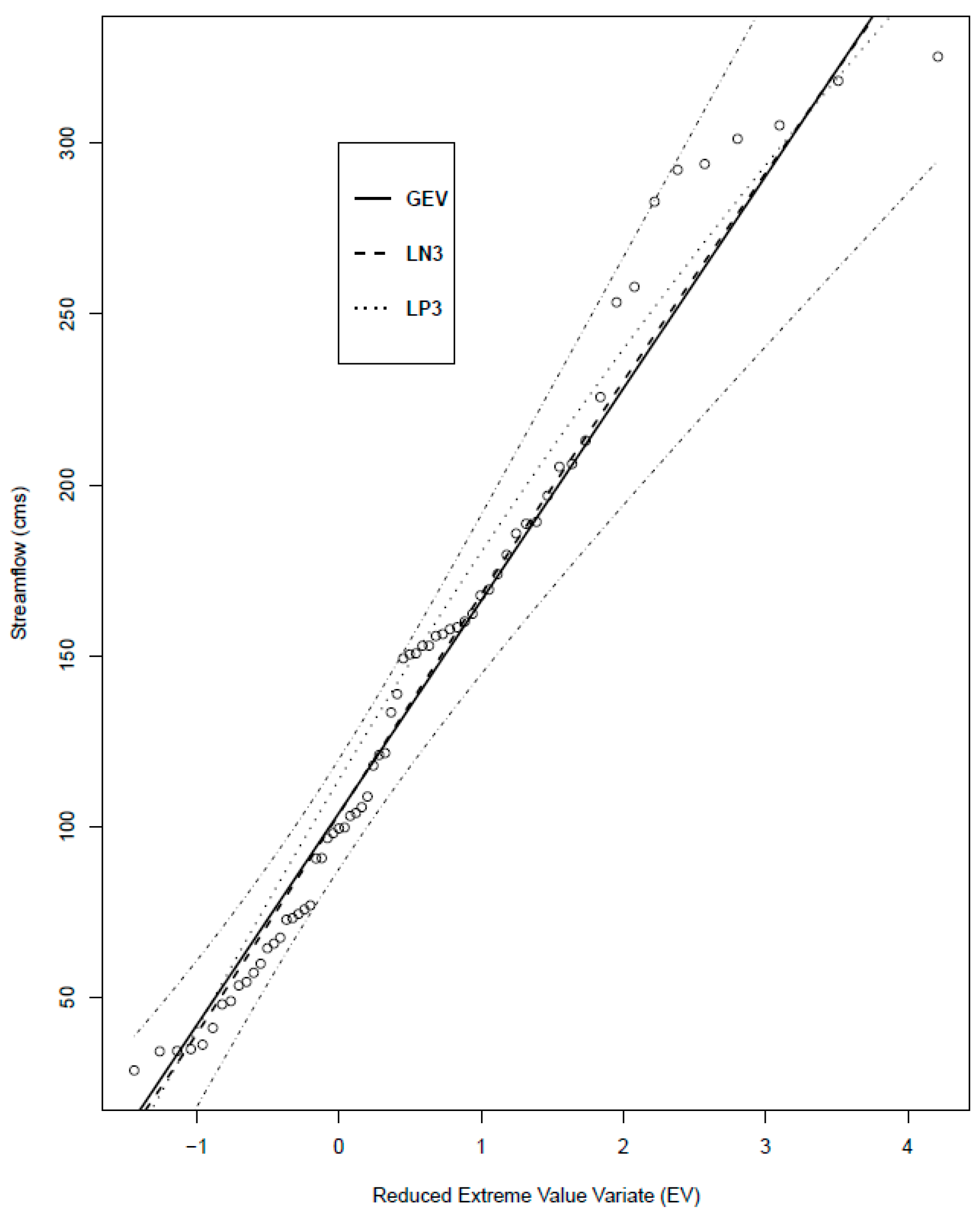
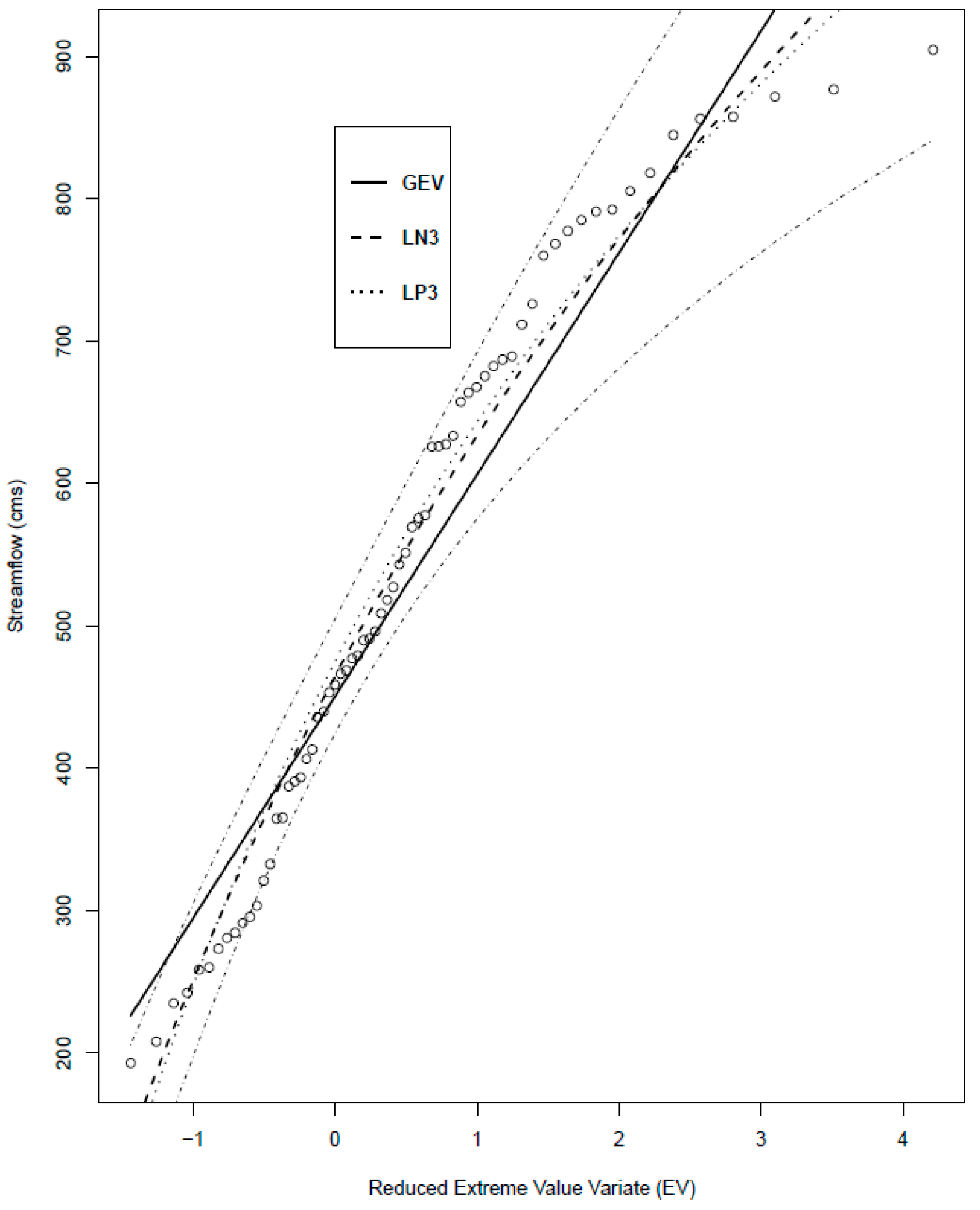
Figure 4, Figure 5 and Figure 6 illustrate a comparison of the 3D flows against the Gumbel reduced variable for the selected USGS OBS1, OB2, and OBS3, respectively. Simple correlation coefficients and Kolmogorov–Smirnov statistic were computed for goodness-of-fit and it is concluded that all three methods are acceptable because the correlation coefficient is high enough (>0.98) and the Kolmogorov–Smimov empirical statistic [48], Dn (Dn = 0.16) is smaller with 95% confidence level. The interested reader may also apply another goodness of fit, such as chi square test [49] for cross validation, when necessary. Confidence limits suggested by [50] were also applied to provide useful insights for water managers, who may utilize this information to mitigate impacts driven by flash floods. Note that the upper and lower bound lines are plotted based on GEV and those lines indicate a wide range of uncertainty for GEV Type I distribution at the 95% confidence level.
The Monte Carlo simulation was also conducted to understand the impact of risk and uncertainty in flash flood events. A total of 1000 streamflow sequences were generated and distinct 30, 60 and 90 samples were selected to observe a 95% confidence level. Table 3 shows the 3D peak flow from Monte Carlo simulation associated with different return periods (25, 50, 100, 150 and 200 years) based on Gumbel Extreme Value Type I (GEV). Note that the return period of 200 years can be interpreted as the total span of streamflow data in BRW has 200-year records from 1951 to 2150 (200 years), which is beyond of the climate model projection until 2099.
The streamflow calibration and validation were also performed to generate climate-induced future streamflows at BRW. The calibration and validation periods of streamflow are 1979–2005 (27 years) and 2006–2015 (10 years), respectively, but the first two years (1979–1980) were used as a warm up period. Table 4 shows the calibration and validation results for performance measures of streamflow at BRW using daily and monthly time steps. Based on criteria and recommended statistics (see Appendix A) for model performances [51,52], all three observed stations, OBS1, OBS2 and OBS3 show good model performance (e.g., R2 = 0.87, NS = 0.86, and RSR = 0.37, and PBIAS = 11.10 at OBS1) during the calibration period. Overall, the calibrated HSPF performs very well to generate climate-driven future streamflows with GCMs inputs.
Table 5 lists the maximum of climate-driven ensemble streamflows (3D flows) from HSPF simulations with GCMs inputs. Both RCP 4.5 and RCP 8.5 scenarios are incorporated into HSPF to explore potential flood risks over the next few decades. It appears that RCP 4.5-induced streamflows might not have a great influence on the difference in the overall 3D flows at the selected stations. However, when the RCP 8.5 scenario was used, the significant increase was observed at OBS2 and OBS3. Based on the flood frequency analysis, the maximum of 3D flows at OBS2 and OBS3 are reported 1471 cms (N = 30) and 1109 cms (N = 3), respectively, which is much less than that from HSPF with GCMs inputs (see Table 5). This implies that uncertainties embedded in GCMs is quite large as opposed to the hydro stationarity—the idea that natural systems fluctuate within an unchanging envelop of historic flow variability [53,54,55]. Such an uncertainty, perhaps, can be reduced through more cohesive joint modeling efforts from the field of climatology and hydrology. Thus, the regional climate models are evolving with additional information and new approaches to better increase the predictability using any large-scale driving data, including aerosols and chemical species [56]. Additionally, the fast-moving technologies and applications, such as high-performance computing, computer parallelism in hydrological modeling [57], and unmanned aerial system (UAS) for flood mapping would be another avenue to improve predictability by mitigating uncertainty and risks associated with other foreseen factors [13] (e.g., population growth, urbanization, and economic development).
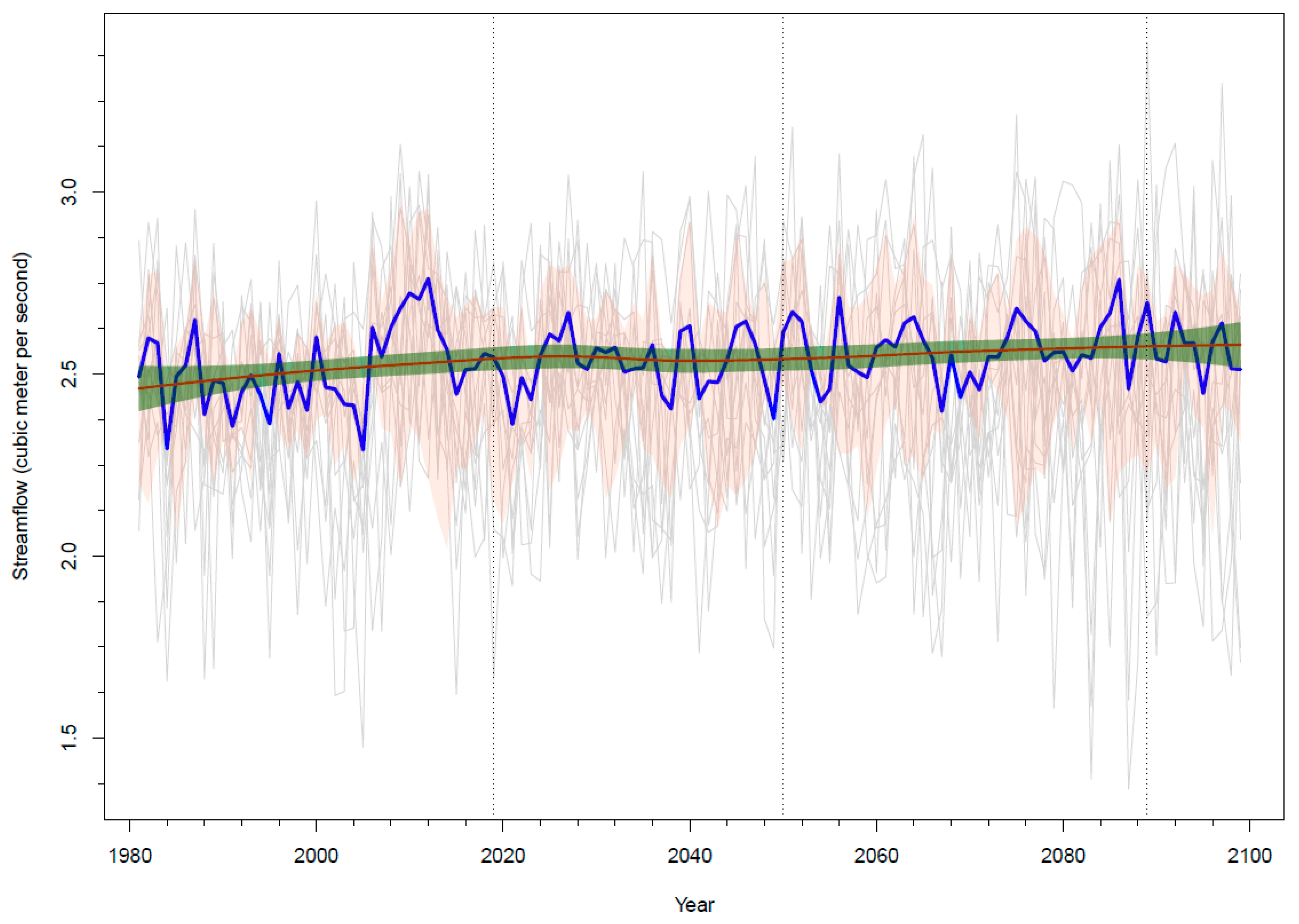
For example, Figure 7, Figure 8 and Figure 9 illustrate the time series of ensemble 3D flows at OBS1, OBS2 and OBS3 respectively from HSPF associated with each of the climate projections. Note that logarithm base 10 is applied to the flow to show general trends of the flow over the next few decades until 2099. One can see that the magnitude of the projected annual 3D peaks varies in different ways for every projection. These peaks would correspond to flash flood values with a return period greater than 140 years when compared to historic observation (1951–2017, 67 years). The linear regression model was then applied to draw a trend line with 95% confidence levels for visual inspection. Additionally, the upper and lower envelop lines indicating 85% and 25% of 3D flows are drawn to provide a general insight for the reader. Unlike 3D flows at OBS1 and OBS2, the climate-driven 3D flows at OBS3 shows an increasing trend with 95% confidence. However, overall climate-driven 3D flows over time get more extreme in the sense that a wider envelop of 3D flow ranges is observed as shown in Figure 7, Figure 8 and Figure 9. Although an uncertainty does still exist in our assumption, the outcome from this research will provide a useful insight for water managers for their future water management practices based on scientific facts rather than personal judgement.
5. Conclusions
We have conducted a study on climate-driven flood risks in the Boise River Watershed using flood frequency analysis and future streamflow ensembles generated by HSPF with climate inputs. Three distribution families, including the Gumbel Extreme Value Type I (GEV), the 3-parameter log-normal (LN3) and log-Pearson type III (LP3) are used to predict future flood risks using a 3-day running total flow (3D flow). In addition to this conventional flood frequency analysis, climate-driven streamflow ensembles are also generated to oversee the likelihood of future flash flood events over the next few decades until 2099. The result indicates that the magnitude of the potential flash flood events is likely increasing over time from both methods, while climate-induced future ensemble streamflows (3D flows) is a broader envelop of historic flow variability. This implies that optimal use of available climate information should be practiced for water managers to plan out their adaptation strategies associated with hydroclimatic nonstationary and uncertainty in a changing global environment. We anticipate that this research will provide useful insights for water stakeholders to make a better decision based on scientific facts rather than personal conjecture. Furthermore, this study can be exemplified to explore future water storage design and management practices in the Boise River Watershed to cope with climate uncertainties.
Author Contributions
J.K. applied HSPF model to generate climate-induced hydrographs and J.H.R. proposed the study and contributed to conceptualizing the project, interpreting the processes in general as J.K.’s advisor.
Funding
This research is supported partially by the National Institute of Food and Agriculture, U.S. Department of Agriculture (USDA), under ID01507 and the Idaho State Board of Education (ISBOE) through IGEM program. Any opinions, findings, conclusions, or recommendations expressed in this publication are those of the authors and do not necessarily reflect the view of USDA and ISBOE.
Conflicts of Interest
The authors declare no conflict of interest.
Appendix A
References
- Das, T.; Maurer, E.P.; Pierce, D.W.; Dettinger, M.D.; Cayan, D.R. Increasing in flood magnitudes in California under warming climates. J. Hydrol. 2013, 501, 101–110. [Google Scholar] [CrossRef]
- Elsner, M.M.; Cuo, L.; Voisin, N.; Deems, J.S.; Hamlet, A.F.; Vano, J.A.; Mickelson, K.E.B.; Lee, S.Y.; Lettenmaier, D.P. Implications of 21st century climate change for the hydrology of Washington State. Clim. Chang. 2010, 102, 225–260. [Google Scholar] [CrossRef] [Green Version]
- Wahl, T.; Jain, S.; Bender, J.; Meyers, S.D.; Luther, M.E. Increasing risk of compound flooding from strom surge and rainfall for major US cities. Nat. Clim. Chang. 2015, 5, 1093–1097. [Google Scholar] [CrossRef]
- Wing, O.E.J.; Bates, P.D.; Smith, A.M.; Sampson, C.C.; Johnson, K.A.; Fargione, J.; Morefield, P. Estimates of present and future flood risk in the conterminous United States. Environ. Res. Lett. 2018, 13, 034023. [Google Scholar] [CrossRef] [Green Version]
- NOAA. Billion-Dollar Weather and Climate Disasters: Table of Events. 2017. Available online: https://www.ncdc.noaa.gov/billions/events/US/2017 (accessed on 28 January 2019).
- Raff, D.A.; Pruitt, T.; Brekke, L.D. A framework for assessing flood frequency based on climate projection information. Hydrol. Earth Syst. Sci. 2009, 13, 2119–2136. [Google Scholar] [CrossRef] [Green Version]
- Clow, D.W. Changes in the Timing of Snowmelt and Streamflow in Colorado: A Response to Recent Warming. J. Clim. 2010, 23, 2293–2306. [Google Scholar] [CrossRef]
- Safeeq, M.; Grant, G.E.; Lewis, S.L.; Tague, C.L. Coupling snowpack and groundwater dynamics to interpret historical streamflow trends in the western United States. Hydrol. Process. 2012, 27, 655–668. [Google Scholar] [CrossRef]
- NWS (National Weather Service). Advanced Hydrologic Prediction Service; 2019. Available online: https://water.weather.gov/ahps2/inundation/index.php?gage=bigi1 (accessed on 1 March 2019).
- Melillo, J.M.; Richmond, T.C.; Yohe, G.W. Climate Change Impacts in the United States: The third national climate assessment. U.S. Glob. Chang. Res. Program 2014, 841. [Google Scholar] [CrossRef]
- Zhou, Q.; Leng, G.; Peng, J. Recent changes in the occurrences and damages of floods and droughts in the United States. Water 2018, 10, 1109. [Google Scholar] [CrossRef]
- Dettinger, M.; Udall, B.; Georgakakos, A. Western water and climate change. Ecol. Appl. 2015, 24, 2069–2093. [Google Scholar] [CrossRef]
- Kim, J.J.; Ryu, J.H. Modeling hydrological and environmental consequences of climate change and urbanization in the Boise River Watershed, Idaho. J. Am. Water Resour. Assoc. 2019, 55, 133–153. [Google Scholar] [CrossRef]
- Pierce, D.W.; Cayan, D.R.; Das, T.; Maurer, E.P.; Miller, N.; Bao, Y.; Kanamitsu, M.; Yoshimura, K.; Snyder, M.A.; Sloan, L.C.; et al. The Key Role of Heavey Precipitation Events in Climate Model disagrremnts of Future Annual Precipitation Changes in California. Am. Meteorol. Soc. 2013, 26, 5879–5896. [Google Scholar]
- USBR. Chapter 2: Hydrology and Climate Assessment. In SECURE Water Act Section 9503(c)—Reclamation Climate Change and Water; United States Bureau of Reclamation: Denver, CO, USA, 2016. [Google Scholar]
- Weil, W.; Jia, F.; Chen, L.; Zhang, H.; Yu, Y. Effects of surficial condition and rainfall intensity on runoff in loess hilly area, China. J. Hydorl. 2014, 56, 115–126. [Google Scholar]
- Miller, M.L.; Palmer, R.N. Developing an Extended Streamflow Forecast for the Pacific Northwest; World Water & Environmental Resources Congress ASCE: Philadelphia, PA, USA, 2003. [Google Scholar]
- Wood, A.W.; Maurer, E.P.; Kumar, A.; Lettenmaier, D.P. Long-Range Experimental Hydrologic Forecasting for the Eastern United States. J. Geophys. Res. 2002, 107, ACL 6-1–ACL 6-15. [Google Scholar] [CrossRef]
- Ryu, J.H. Application of HSPF to the Distributed Model Intercomparison Project: Case Study. J. Hydrol. Eng. 2009, 14, 847–857. [Google Scholar] [CrossRef]
- Quintero, F.; Mantilla, R.; Anderson, C.; Claman, D.; Krajewski, W. Assessment of Changes in Flood Frequency Due to the Effects of Climate Change: Implications for Engineering Design. Hydrology 2018, 5, 19. [Google Scholar] [CrossRef]
- IDEQ. Lower Boise River Nutrient Subbasin Assessment; Idaho Department of Environmental Quality: Boise, ID, USA, 2001; pp. 18–19.
- Carlson, B. Proposal to Raise One of Three Boise River Dams Favors Anderson Ranch. Available online: https://www.capitalpress.com/state/idaho/proposal-to-raise-one-of-three-boise-river-dams-favors/article_52d1f19f-fbed-5843-9736-7cb3174b1573.html (accessed on 15 March 2019).
- Tasker, G.D. A Comparison of methods for estimating low flow characterisics of streams. J. Am. Water Resour. Assoc. 1987, 23, 1077–1083. [Google Scholar] [CrossRef]
- Loganathan, G.V. Frequency analysis of low flows. Nord. Hydrol. 1985, 17, 129–150. [Google Scholar] [CrossRef]
- Matalas, N.C. Probability distribution of low flows, Statistical Studies in Hydrology. In Geological Survey Professional Paper 434-A; 1963. Available online: https://pubs.usgs.gov/pp/0434a/report.pdf (accessed on 1 March 2019).
- Ryu, J.H.; Lee, J.H.; Jeong, S.; Park, S.K.; Han, K. The impacts of climate change on local hydrology and low flow frequency in the Geum River Basin, Korea. Hydrol. Process. 2011, 25, 3437–3447. [Google Scholar] [CrossRef]
- Linsley, R.K.; Kohler, M.A.; Paulhus, J.L.H. Hydrology for Engineers; McGraw-Hill: New York, NY, USA, 1982. [Google Scholar]
- Stedinger, J.R.; Vogel, R.M.; Efi, F.-G. Handbook of Hydrology; Maidment, D., Ed.; McGraw-Hill: New York, NY, USA, 1993; pp. 18.12–18.13. [Google Scholar]
- Weibull, W.A. Statistical Theory of the Strength of Materials; the Royal Swedish Institute for Engineering Research: Stockholm, Swedish, 1939. [Google Scholar]
- Chow, V.T. A general formula for hydrologic frequency analysis. Trans. Am. Geophys. Union 1951, 32, 231–237. [Google Scholar] [CrossRef]
- Fisher, R.A.; Tippett, L.H.C. Limiting Forms of the Frequency Distributions of the Smalles and Largest Member of a Sample. Proc. Camb. Philos. Soc. 1928, 24, 180–190. [Google Scholar] [CrossRef]
- Hosking, J.R.M.; Wallis, J.R.; Wood, A.W. Estimation of the Generalized Extreme Value Distribution by the Method of Probability-Weighted Moments. Technometrics 1985, 27, 251–261. [Google Scholar] [CrossRef]
- Hoshi, K.; Stedinger, J.R.; Burges, S.J. Estimation of Log-Normal Quantiles: Monte Carlo Results and First-Order Approximations. J. Hydrol. 1984, 71, 1–30. [Google Scholar] [CrossRef]
- Stedinger, J.R. Fitting Log Normal Distributions to Hydrologic Data. Water Resour. Res. 1980, 16, 481–490. [Google Scholar] [CrossRef]
- Bobee, B. The Log Pearson Type 3 Distribution and Its Application in Hydrology. Water Resour. Res. 1975, 11, 681–689. [Google Scholar] [CrossRef]
- Dudula, J.; Randhir, T.O. Modeling the influence of climate change on watershed systems: Adaptation through targeted practices. J. Hydrol. 2016, 541, 703–713. [Google Scholar] [CrossRef]
- Tong, S.T.Y.; Ranatunga, T.; He, J.; Yang, T.J. Predicting plausible impacts of sets of climate and land use change scenarios on water resources. Appl. Geogr. 2012, 32, 477–489. [Google Scholar] [CrossRef]
- Stern, M.; Flint, L.; Minear, J.; Flint, A.; Wright, S. Characterizing Changes in Streamflow and Sediment Supply in the Sacramento River Basin, California, Using Hydrological Simulation Program-Fortran (HSPF). Water 2016, 8, 432. [Google Scholar] [CrossRef]
- Bicknell, B.; Imhoff, J.; Kittle, J., Jr.; Jones, T.; Donigian, A., Jr.; Johanson, R. Hydrological Simulation Program-FORTRAN: HSPF Version 12 User’s Manual; AQUA TERRA Consultants: Mountain View, CA, USA, 2001. [Google Scholar]
- Crawford, N.H.; Linsley, R.K. Digital Simulation in Hydrology: Stanford Watershed Model IV; Technical Report No. 39; Department of Civil Engineering, Stanford University: Stanford, CA, USA, 1966. [Google Scholar]
- Donigian, A.S.; Davis, H.H. User’s Manual for Agricultural Runoff Management (ARM) Model; The National Technical Information Service: Springfield, VA, USA, 1978.
- Donigian, A.S.; Crawford, N.H. Modeling Nonpoint Pollution from the Land Surface; US Environmental Protection Agency, Office of Research and Development, Environmental Research Laboratory: Washington, DC, USA, 1976.
- Donigian, A.S.; Huber, W.C.; Laboratory, E.R.; Consultants, A.T. Modeling of Nonpoint Source Water Quality in Urban and Non-urban Areas; US Environmental Protection Agency, Office of Research and Development, Environmental Research Laboratory: Washington, DC, USA, 1991.
- Donigian, A., Jr.; Bicknell, B.; Imhoff, J.; Singh, V. Hydrological Simulation Program-Frotran (HSPF). In Computer Models of Watershed Hydrology; Water Resources Publications: Highlands Ranch, CO, USA, 1995; pp. 395–442. [Google Scholar]
- Kim, J.J.; Ryu, J.H. A threshold of basin discretization for HSPF simulations with NEXRAD inputs. J. Hydrol. Eng. 2013, 19, 1401–1412. [Google Scholar] [CrossRef]
- Mitchell, K.E.; Lohmann, D.; Houser, P.R.; Wood, E.F.; Schaake, J.C.; Robock, A.; Cosgrove, B.A.; Sheffield, J.; Duan, Q.Y.; Luo, L.; et al. The multi-institution North American Land Data Assimilation System (NLDAS): Utilizaing multiple GCIP products and partners in a continental distributed hydrologicl modeling system. J. Geophys. Res. 2004, 109, D07S90. [Google Scholar] [CrossRef]
- Abatzoglou, J.T. Development of gridded surface meteorological data for ecological applications and modeling. Int. J. Climatol. 2011, 33, 121–131. [Google Scholar] [CrossRef]
- Fasano, G.; Franceschini, A. A multivariate version of the Kolmogorov-Sminov test. Mon. Not. R. Astron. Soc. 1987, 225, 155–170. [Google Scholar] [CrossRef]
- Benjamin, J.R.; Cornell, C.A. Probability, Statistics and Decision for Civil Engineers; McGraw-Hill: New York, NY, USA, 1970; 684p. [Google Scholar]
- Kite, G.W. Confidence limits for design events. Water Resour. Res. 1975, 11, 48–53. [Google Scholar] [CrossRef]
- Duda, P.B.; Hummel, P.R.; Donigian, A.S., Jr.; Imhoff, J.C. BASINS/HSPF: Model use, calibration, and validation. Trans. ASABE 2012, 55, 1523–1547. [Google Scholar] [CrossRef]
- Moriasi, D.N.; Arnold, J.G.; Van Liew, M.W.; Binger, R.L.; Harmel, R.D.; Veith, T.L. Model Evaluation Guidelines for Systematic Quantification of Accuracy in Watershed Simulations. Am. Soc. Agric. Biol. Eng. 2007, 50, 885–900. [Google Scholar] [CrossRef]
- Milly, P.C.D.; Betancourt, J.; Falkenmark, M.; Hirsch, R.M.; Kundzewicz, Z.W.; Letternmaier, D.P. Stationarity Is Dead: Whiher Water Management? Science 2008, 319, 573–574. [Google Scholar] [CrossRef]
- Veldkamp, T.; Frieler, K.; Schewe, J.; Ostberg, S.; Willner, S.; Schauberger, B.; Gosling, S.N.; Schmied, H.M.; Portmann, F.T.; Huang, M.; et al. The critical role of the routing scheme in simulating peak river discharge in global hydrological models. Environ. Res. Lett. 2017, 12, 075003. [Google Scholar]
- Liu, S.; Huang, S.; Xie, Y.; Wang, H.; Leng, G.; Huang, Q.; Wei, X.; Wang, L. Identification of the non-stationarity of floods: Changing patterns, causes, and implications. Water Resour. Manag. 2019, 33, 939–953. [Google Scholar] [CrossRef]
- Fcinocca, J.F.; Kharin, V.V.; Jiao, Y.; Qian, M.W.; Lazare, M.; Solheim, L.; Flato, G.M.; Biner, S.; Desgagne, M.; Dugas, B. Coordinated global and regional climate modeling. J. Clim. 2016, 29, 17–35. [Google Scholar] [CrossRef]
- Kim, J.J.; Ryu, J.H. Quantifying the performances of the semi-distributed hydrologic model in parallel computing—A case study. Water 2019, 11, 823. [Google Scholar] [CrossRef]
- Santhi, C.; Arnold, J.G.; Williams, J.R.; Dugas, W.A.; Srinivasan, R.; Hauck, L.M. Validation of the SWAT Model on a Large River Basin with Point and Nonpoint Sources. J. Am. Water Resour. Assoc. 2001, 37, 1169–1188. [Google Scholar] [CrossRef]
- Nash, J.E.; Sutcliffe, J.V. River flow forecasting through conceptual models: Part I—A discussion of principles. J. Hydrol. 1970, 10, 282–290. [Google Scholar] [CrossRef]
- Legates, D.R.; McCabe, G.J. Evaluating the Use of ‘Goodness-of-Fit’ Measures in Hydrologic and Hydroclimatic Model Validation. Water Resour. Res. 1999, 35, 233–241. [Google Scholar] [CrossRef]
- Gupta, I.; Gupta, A.; Khanna, P. Genetic algorithm for optimization of water distribution system. Environ. Model. Softw. 1999, 14, 437–446. [Google Scholar] [CrossRef]
Figure 1.
Map of the Boise River Watershed.

Figure 2.
Box plots of the observed seasonal streamflow at the selected United States Geological Survey (USGS) stations (OBS1: USGS 1320000, OBS2: USGS 13185000, OBS3: USGS 13186000).
Figure 2.
Box plots of the observed seasonal streamflow at the selected United States Geological Survey (USGS) stations (OBS1: USGS 1320000, OBS2: USGS 13185000, OBS3: USGS 13186000).

Figure 3.
The number of occurrences of the maximum 3-day running total streamflow sequences (3D flows) at the given year for January 1 1951 to December 31 2017 at the selected USGS stations (OBS1: USGS 1320000, OBS2: USGS 13185000, OBS3: USGS 13186000).
Figure 3.
The number of occurrences of the maximum 3-day running total streamflow sequences (3D flows) at the given year for January 1 1951 to December 31 2017 at the selected USGS stations (OBS1: USGS 1320000, OBS2: USGS 13185000, OBS3: USGS 13186000).

Figure 4.
Comparison of three theoretical distributions (Gumbel Extreme Value Type I (GEV), 3-parameter log-normal (LN3), log-Pearson type III (LP3)) for annual 3D flow frequency at the 95% confidence level at OBS1 (USGS 13200000).
Figure 4.
Comparison of three theoretical distributions (Gumbel Extreme Value Type I (GEV), 3-parameter log-normal (LN3), log-Pearson type III (LP3)) for annual 3D flow frequency at the 95% confidence level at OBS1 (USGS 13200000).

Figure 5.
Comparison of three theoretical distributions (GEV, LN3, LP3) for annual 3D flow frequency at the 95% confidence level at OBS2 (USGS 13185000).
Figure 5.
Comparison of three theoretical distributions (GEV, LN3, LP3) for annual 3D flow frequency at the 95% confidence level at OBS2 (USGS 13185000).

Figure 6.
Comparison of three theoretical distributions (GEV, LN3, LP3) for annual 3D flow frequency at the 95% confidence level at OBS3 (USGS 13186000).
Figure 6.
Comparison of three theoretical distributions (GEV, LN3, LP3) for annual 3D flow frequency at the 95% confidence level at OBS3 (USGS 13186000).

Figure 7.
The climate-driven ensemble 3D flows at OBS1.

Figure 8.
The climate-driven ensemble 3D flows at OBS2.

Figure 9.
The climate-driven ensemble 3D flows at OBS3.


Table 1.
The 3-day running total streamflows at the selected USGS stations (OBS1: USGS 13200000, OBS2: USGS 13185000, OBS3: USGS 13186000).
Table 1.
The 3-day running total streamflows at the selected USGS stations (OBS1: USGS 13200000, OBS2: USGS 13185000, OBS3: USGS 13186000).
| Index | OBS1 | OBS2 | OBS3 | |||
|---|---|---|---|---|---|---|
| Date | Flow | Date | Flow | Date | Flow | |
| 1 | 7 April 1951 | 179.53 | 28 May 1951 | 551.33 | 28 May 1951 | 420.79 |
| 2 | 27 April 1952 | 282.88 | 27April 1952 | 686.97 | 4 May1952 | 430.42 |
| 3 | 28 April 1953 | 133.37 | 13 June 1953 | 626.08 | 13June 1953 | 352.26 |
| 4 | 18 April 1954 | 121.48 | 20 May 1954 | 625.80 | 20 May 1954 | 408.89 |
| 5 | 23 December 1955 | 292.23 | 23 December 1955 | 575.68 | 10 June 1955 | 306.67 |
| 6 | 16 April 1956 | 189.16 | 24 May 1956 | 857.43 | 24 May 1956 | 592.67 |
| 7 | 30 May 1970 | 149.23 | 5 June 1957 | 663.75 | 5 June 1957 | 473.74 |
| 8 | 18 April 1958 | 162.26 | 21 May 1958 | 818.07 | 22 May 1958 | 609.94 |
| 9 | 6 April 1959 | 90.61 | 14 June 1959 | 390.77 | 14 June 1959 | 235.31 |
| 10 | 7 April 1960 | 150.65 | 12 May 1960 | 458.73 | 12 May 1960 | 318.85 |
| 11 | 4 April 1961 | 53.43 | 26 May 1961 | 364.72 | 26 May 1961 | 216.34 |
| 12 | 19 April 1970 | 108.74 | 20 April 1962 | 393.60 | 12 June 1962 | 281.19 |
| 13 | 7 April 1963 | 73.14 | 24 May 1963 | 453.35 | 24 May 1963 | 326.21 |
| 14 | 24 December 1964 | 305.26 | 24 December 1964 | 777.30 | 21 May 1964 | 281.19 |
| 15 | 23 April 1965 | 325.36 | 11 June 1965 | 682.43 | 11 June 1965 | 550.76 |
| 16 | 1 April 1966 | 64.34 | 8 May 1966 | 321.11 | 9 May 1966 | 233.05 |
| 17 | 23 May 1967 | 72.69 | 23 May 1967 | 577.66 | 24 May 1967 | 466.09 |
| 18 | 23 February 1968 | 74.39 | 4 June 1968 | 295.63 | 4 June 1968 | 180.09 |
| 19 | 6 April 1969 | 205.30 | 14 May 1969 | 543.12 | 14 May 1969 | 480.54 |
| 20 | 24 May 1970 | 103.92 | 26 May 1970 | 569.45 | 8 June 1970 | 382.84 |
| 21 | 5 May 1971 | 185.76 | 14 May 1971 | 667.71 | 13 May 1971 | 518.48 |
| 22 | 19 March 1972 | 188.59 | 2 June 1972 | 784.94 | 9 June 1972 | 510.27 |
| 23 | 15 April 1973 | 54.45 | 19 May 1973 | 435.80 | 19 May 1973 | 257.40 |
| 24 | 31 March 1974 | 206.15 | 16 June 1974 | 805.33 | 16 June 1974 | 485.35 |
| 25 | 16 May 1975 | 225.68 | 16 May 1975 | 627.50 | 7 June 1975 | 467.51 |
| 26 | 10 April 1976 | 156.31 | 12 May 1976 | 527.26 | 15 May 1976 | 335.27 |
| 27 | 16 December 1977 | 76.88 | 16 December 1977 | 208.13 | 10 June 1977 | 60.37 |
| 28 | 31 March 1978 | 159.99 | 9 June 1978 | 496.11 | 9 June 1978 | 358.21 |
| 29 | 17 May 1979 | 48.85 | 25 May 1979 | 406.63 | 25 May 1979 | 266.18 |
| 30 | 24 April 1980 | 138.75 | 6 May 1980 | 491.01 | 6 May 1980 | 334.14 |
| 31 | 21 April 1981 | 65.69 | 9 June 1981 | 413.14 | 9 June 1981 | 240.41 |
| 32 | 14 April 1982 | 212.94 | 25 May 1982 | 633.45 | 18 June 1982 | 503.19 |
| 33 | 13 March 1983 | 257.97 | 29 May 1983 | 871.59 | 29 May 1983 | 643.36 |
| 34 | 18 April 1984 | 196.80 | 15 May 1984 | 711.60 | 15 May 1984 | 496.96 |
| 35 | 11 April 1985 | 120.91 | 4 May 1985 | 332.72 | 25 May 1985 | 244.09 |
| 36 | 24 February 1986 | 253.44 | 31 May 1986 | 768.23 | 31 May 1986 | 557.27 |
| 37 | 14 March 1987 | 47.91 | 30 April 1987 | 242.39 | 30 April 1987 | 146.40 |
| 38 | 5 April 1988 | 41.00 | 25 May 1988 | 260.23 | 25 May 1988 | 177.26 |
| 39 | 20 April 1989 | 155.74 | 10 May 1989 | 466.38 | 10 May 1989 | 342.35 |
| 40 | 29 April 1990 | 98.00 | 29 April 1990 | 280.90 | 31 May 1990 | 167.92 |
| 41 | 18 May 1991 | 34.26 | 4 June 1991 | 258.53 | 12 June 1991 | 179.53 |
| 42 | 22 February 1992 | 36.10 | 8 May 1992 | 193.12 | 8 May 1992 | 116.10 |
| 43 | 5 April 1993 | 167.64 | 15 May 1993 | 675.36 | 21 May 1993 | 390.49 |
| 44 | 22 April 1994 | 28.57 | 12 May 1994 | 235.03 | 13 May 1994 | 137.62 |
| 45 | 8 April 1995 | 150.36 | 4 June 1995 | 518.20 | 4 June 1995 | 425.32 |
| 46 | 31 December 1996 | 152.88 | 16 May 1996 | 790.89 | 17 May 1996 | 552.74 |
| 47 | 2 January 1997 | 301.29 | 16 May 1997 | 856.02 | 17 May 1997 | 656.10 |
| 48 | 28 May 1998 | 169.33 | 27 May 1998 | 468.64 | 10 May 1998 | 312.62 |
| 49 | 20 April 1999 | 158.29 | 26 May 1999 | 657.23 | 26 May 1999 | 438.06 |
| 50 | 14 April 2000 | 90.73 | 24 May 2000 | 387.37 | 24 May 2000 | 255.42 |
| 51 | 25 March 2001 | 34.15 | 16 May 2001 | 273.26 | 16 May 2001 | 140.45 |
| 52 | 15 April 2002 | 157.72 | 15 April 2002 | 479.12 | 1 June 2002 | 280.34 |
| 53 | 27 March 2003 | 67.42 | 30 May 2003 | 689.23 | 30 May 2003 | 467.51 |
| 54 | 7 April 2004 | 99.39 | 5 June 2004 | 284.58 | 6 May 2004 | 171.03 |
| 55 | 20 May 2005 | 59.81 | 20 May 2005 | 477.14 | 20 May 2005 | 381.99 |
| 56 | 6 April 2006 | 293.93 | 20 May 2006 | 844.69 | 20 May 2006 | 651.85 |
| 57 | 14 March 2007 | 57.14 | 2 May 2007 | 291.38 | 13 May 2007 | 152.63 |
| 58 | 20 May 2008 | 105.62 | 20 May 2008 | 760.02 | 20 May 2008 | 412.86 |
| 59 | 22 April 2009 | 96.56 | 20 May 2009 | 508.85 | 1 June 2009 | 325.36 |
| 60 | 6 June 2010 | 103.07 | 6 June 2010 | 726.04 | 6 June 2010 | 413.99 |
| 61 | 18 April 2011 | 152.91 | 15 May 2011 | 792.30 | 15 May 2011 | 416.82 |
| 62 | 1 April 2012 | 173.87 | 27 April 2012 | 904.44 | 26 April 2012 | 538.02 |
| 63 | 7 April 2013 | 34.77 | 14 May 2013 | 365.29 | 14 May 2013 | 220.02 |
| 64 | 11 March 2014 | 75.69 | 27 May 2014 | 489.88 | 27 May 2014 | 274.39 |
| 65 | 10 February 2015 | 117.80 | 9 February 2015 | 303.56 | 26 May 2015 | 160.84 |
| 66 | 14 March 2016 | 99.68 | 13 April 2016 | 439.76 | 13 April 2016 | 298.46 |
| 67 | 21 March 2017 | 318.28 | 7 May 2017 | 876.69 | 7 May 2017 | 813.54 |
Table 2.
List of the Coupled Model Inter-Comparison Project (CMIP5) models used in this study.
| Model | Modeling Group | Note |
|---|---|---|
| BCC-CSM1-1 | Beijing Climate Center, China Meteorological Administration, China | 1. 4 km spatial resolution 2. Scenario: RCP4.5, RCP8.5 |
| BCC-CSM1-1m | ||
| BNU-ESM | College of Global Change and Earth System Science, Beijing Normal University, China | |
| CANESM2 | Canadian Centre for Climate Modelling and Analysis, Canada | |
| CCSM4 | National Center for Atmospheric Research, USA | |
| CNRM-CM5 | Centre National de Recherches Meteorologiques, Meteo-France, France | |
| CSIRO-MK3 | Commonwealth Scientific and Industrial Research Organisation in collaboration with the Queensland Climate Change Centre of Excellence, Australia | |
| GFDL-ESM2G | NOAA Geophysical Fluid Dynamics Laboratory (GFDL), USA | |
| IPSL-CM5A-LR | Institute Pierre-Simon Laplace, France | |
| IPSL-CM5A-MR | ||
| IPSL-CM5B-LR | ||
| MIROC5 | Atmosphere and Ocean Research Institute, Japan | |
| MIROC-ESM | Japan Agency for Marine-Earth Science and Technology, Japan | |
| MIROC-ESM-CHEM |
Table 3.
The 3D peak flows from Monte Carlo simulation from 1000 streamflow sequences with different sample sizes (30, 60, 90) and return periods (25, 50, 100, and 200 years) based on Gumbel Extreme Value Type I (GEV).
Table 3.
The 3D peak flows from Monte Carlo simulation from 1000 streamflow sequences with different sample sizes (30, 60, 90) and return periods (25, 50, 100, and 200 years) based on Gumbel Extreme Value Type I (GEV).
| OBS1 | 25 | 50 | 100 | 150 | 200 | |
| N = 30 | Upper | 348 | 410 | 458 | 486 | 514 |
| Lower | 255 | 285 | 319 | 337 | 353 | |
| N = 60 | Upper | 336 | 390 | 437 | 464 | 491 |
| Lower | 268 | 302 | 341 | 358 | 380 | |
| N = 90 | Upper | 333 | 381 | 426 | 458 | 480 |
| Lower | 274 | 313 | 352 | 374 | 386 | |
| OBS2 | 25 | 50 | 100 | 150 | 200 | |
| N = 30 | Upper | 1075 | 1206 | 1337 | 1425 | 1471 |
| Lower | 822 | 918 | 983 | 1039 | 1067 | |
| N = 60 | Upper | 1033 | 1166 | 1278 | 1371 | 1422 |
| Lower | 858 | 952 | 1044 | 1093 | 1123 | |
| N = 90 | Upper | 1025 | 1143 | 1268 | 1337 | 1402 |
| Lower | 876 | 972 | 1062 | 1118 | 1164 | |
| OBS3 | 25 | 50 | 100 | 150 | 200 | |
| N = 30 | Upper | 780 | 884 | 985 | 1076 | 1109 |
| Lower | 587 | 654 | 714 | 761 | 780 | |
| N = 60 | Upper | 753 | 854 | 950 | 1013 | 1053 |
| Lower | 612 | 686 | 759 | 805 | 829 | |
| N = 90 | Upper | 739 | 842 | 929 | 994 | 1029 |
| Lower | 628 | 705 | 781 | 822 | 844 | |
Table 4.
Performance statistics for the calibrated (1979–2005) and validated (2006–2015) monthly streamflow at the Boise River Watershed using daily and monthly time steps.
Table 4.
Performance statistics for the calibrated (1979–2005) and validated (2006–2015) monthly streamflow at the Boise River Watershed using daily and monthly time steps.
| Variable | OBS1 | OBS2 | OBS3 | ||||
|---|---|---|---|---|---|---|---|
| Cal | Val | Cal | Val | Cal | Val | ||
| R2 | Daily | 0.82 | 0.72 | 0.78 | 0.74 | 0.81 | 0.87 |
| Monthly | 0.87 | 0.81 | 0.85 | 0.80 | 0.85 | 0.92 | |
| NS | Daily | 0.81 | 0.70 | 0.77 | 0.73 | 0.79 | 0.86 |
| Monthly | 0.86 | 0.87 | 0.85 | 0.89 | 0.84 | 0.95 | |
| RSR | Daily | 0.43 | 0.54 | 0.48 | 0.52 | 0.46 | 0.37 |
| Monthly | 0.37 | 0.36 | 0.39 | 0.34 | 0.40 | 0.22 | |
| PBIAS (%) | Daily | 11.11 | 17.35 | 7.82 | 3.19 | 9.74 | 1.50 |
| Monthly | 11.10 | 17.41 | 7.77 | 3.18 | 9.79 | 1.64 | |
Table 5.
The maximum of 3D flow from Hydrological Simulation Program FORTRAN (HSPF) simulations with Global Circulation Models (GCMs) inputs.
Table 5.
The maximum of 3D flow from Hydrological Simulation Program FORTRAN (HSPF) simulations with Global Circulation Models (GCMs) inputs.
| Climate Scenario | USGS Station | Streamflow | Date | Climate Model |
|---|---|---|---|---|
| RCP 4.5 | OBS1 | 985.83 | 30 December 2011 | Ipsl.cm5a |
| OBS2 | 2469.16 | 30 December 2011 | Ipsl.cm5a | |
| OBS3 | 1777.35 | 8 February 2015 | Bcc.scm1 | |
| RCP 8.5 | OBS1 | 776.65 | 16 March 1998 | Ipsl.cm5b |
| OBS2 | 1636.52 | 9 January 2089 | Canesm2 | |
| OBS3 | 2563.15 | 18 January 2089 | Canesm2 |
© 2019 by the authors. Licensee MDPI, Basel, Switzerland. This article is an open access article distributed under the terms and conditions of the Creative Commons Attribution (CC BY) license (http://creativecommons.org/licenses/by/4.0/).
Share and Cite
MDPI and ACS Style
Ryu, J.H.; Kim, J. A Study on Climate-Driven Flash Flood Risks in the Boise River Watershed, Idaho. Water 2019, 11, 1039. https://doi.org/10.3390/w11051039
AMA Style
Ryu JH, Kim J. A Study on Climate-Driven Flash Flood Risks in the Boise River Watershed, Idaho. Water. 2019; 11(5):1039. https://doi.org/10.3390/w11051039
Chicago/Turabian StyleRyu, Jae Hyeon, and Jungjin Kim. 2019. "A Study on Climate-Driven Flash Flood Risks in the Boise River Watershed, Idaho" Water 11, no. 5: 1039. https://doi.org/10.3390/w11051039
Note that from the first issue of 2016, this journal uses article numbers instead of page numbers. See further details here.