Soil Water Content Estimation Using High-Frequency Ground Penetrating Radar


1
State Key Laboratory of Simulation and Regulation of Water Cycle in River Basin, China Institute of Water Research and Hydropower Research, Beijing 100048, China
2
State Key Laboratory of Soil Sustainable Agriculture, Institute of Soil Science, Chinese Academy of Sciences, Nanjing 210008, China
3
Research Center of Water and Soil Conservation Ecological Engineering and Technology, Beijing 100048, China
*
Author to whom correspondence should be addressed.
Water 2019, 11(5), 1036; https://doi.org/10.3390/w11051036
Submission received: 29 March 2019
/
Revised: 14 May 2019
/
Accepted: 15 May 2019
/
Published: 17 May 2019
(This article belongs to the Special Issue Ecohydrologic Feedbacks between Vegetation, Soil, and Climate)
Abstract
:The rapid high-precision and nondestructive determination of shallow soil water content (SWC) is of vital importance to precision agriculture and water resource management. However, the low-frequency ground penetrating radar (GPR) technology currently in use is insufficient for precisely determining the shallow SWC. Therefore, it is essential to develop and use a high-precision detection technology to determine SWC. In this paper, a laboratory study was conducted to evaluate the use of a high-frequency GPR antenna to determine the SWC of loamy sand, clay, and silty loam. We collected soil samples (0–20 cm) of six soil types of loamy sand, clay, and silty loam and used a high-frequency (2-GHz) GPR antenna to determine the SWC. In addition, we obtained GPR data and images as well as characteristic parameters of the electromagnetic spectrum and analyzed the quantitative relationship with SWC. The GPR reflection two-way travel times and the known depths of reflectors were used to calculate the average soil dielectric permittivities above the reflectors and establish a spatial relationship between the soil dielectric permittivity () and SWC (), which was used to estimate the depth-averaged SWC. The results show that the SWC, which affects the attenuation of wave energy and the wave velocity of the GPR signal, is a dominant factor affecting the soil dielectric permittivity. In addition, the conductivity, magnetic soil, soil texture, soil organic matter, and soil temperature have substantial effects on the soil dielectric permittivity, which consequentially affects the prediction of SWC. The correlation coefficients R2 of the cubic curve models, which were used to fit the relationships between the soil dielectric permittivity () and SWC (), were greater than 0.89, and the root-mean-square errors were less than 2.9%, which demonstrate that high-frequency GPR technology can be applied to determine shallow SWC under variable hydrological conditions.
1. Introduction
The shallow soil water content (SWC) is the water in the upper 20 cm of soil. Compared with the total amount of water on the global scale, this thin layer of soil water may appear to be insignificant; however, it is of fundamental importance to many hydrological, biological, and biogeochemical processes. The rapid, high-precision, and nondestructive determination of shallow SWC is of vital importance in developing precision agriculture and preventing slope soil erosion [1]. The SWC determines the conversion of precipitation into surface runoff and infiltration, thus affecting soil erosion, river recharge, and groundwater recharge [2]. At the field scale, the SWC controls plant growth and crop quality [3]. With too much water, crop quality can decrease due to the adverse effects of waterlogged plant roots. With too little water, crops can be irreversibly damaged due to drought stress [4]. Consequently, agronomists and farmers need information about shallow SWC variability at both spatial and temporal scales in cultivated regions to manage irrigation practices effectively [5,6]. However, variations in soil texture, topography, geology, tillage, vegetation cover, and irrigation practices result in large spatial and temporal variabilities in shallow SWC [2]. Therefore, rapid, continuous and reliable estimation of shallow SWC is necessary to achieve effective soil water management at the field scale. Existing methods to characterize shallow SWC are either suited to small scales (<0.1 m), such as the gravimetric method, time-domain-reflectometry (TDR), and capacitive sensors, or to large areas (>10–100 m), such as remote sensing and airborne and spaceborne passive microwave and active radar systems [7]. Below, we briefly describe these methods for measuring shallow SWC.
At small scales, the gravimetric method involves samples being weighed, dried for 6–8 h at 105 °C to reach a constant weight, and being reweighed to calculate the SWC [8,9]. Although this approach is simple, highly precise (1%), and inexpensive, it destroys the soil structure and requires large amounts of time and labor [8]. Moreover, it does not allow for replication at the same location and does not provide SWC profile information of the entire area; it only provides SWC estimates at individual points and cannot be applied continuously over large scales. The TDR method uses the principle of electromagnetic pulses to indirectly measure the effective soil dielectric permittivity and then predicts SWC via an empirical equation [10]. TDR data collection is easily automated, which makes it an ideal technique for monitoring SWC variability at high temporal resolutions [11]. However, because of the small measurement volume of TDR probes, a large number of probes are needed for good spatial coverage, and the probes destroy the soil structure. Moreover, the measurement results are easily affected by soil voids and are not suitable for saline-alkaline soils [12].
At large scales, remote sensing with either passive microwave radiometry or active radar instruments is the most promising technique for measuring SWC variations [4,13]. Because remote sensing does not measure SWC directly, mathematical models that describe the relationship between the measured signal and SWC must be derived [14,15]. Passive microwaves have low atmospheric noise and low spatial resolution, so their application range is tens of square kilometers. Active microwaves have smaller swath widths ranging from 1 to several 1000 m2 due to their long wavelength, strong penetration capacity, and are not affected by the weather conditions [16]. Because remote sensing approaches are used to estimate SWC in the uppermost 5 cm of the soil, they require that the vegetation cover be minimal, cannot measure soil ice, and are sensitive to surface roughness, and the satellite missions have discontinuous temporal coverages and short life spans, which are not suitable for agricultural sites [17,18,19].
Clearly, there is a scale gap between point measurements and remote sensing measurements of SWC. For intermediate scales, such as agricultural land and small catchments, it is urgent to develop a technical method that is rapid and can continuously measure SWC. Recently, remote and proximal sensing techniques are emerging as new innovative and contactless methods for SWC monitoring at a field scale. These methods include cosmic-ray neutron sensing, satellite images, proximal gamma ray spectroscopy, and ground penetrating radar (GPR). The cosmic-ray method is based on the inverse relationship between the inverse neutron intensity of cosmic rays above the surface and the SWC; a neutron probe mounted above the surface of the earth is used to measure the intensity of fast neutrons, which is inverted for the shallow SWC [20]. This method has several useful features: it is noninvasive and noncontact, does not use a radioactive source, can be automated easily, consumes little energy, and is compatible with low data stream telemetry techniques [19]. Among the proximal sensing techniques, gamma ray spectroscopy is recognized as having one of the best space-time tradeoffs for measuring shallow SWC. Proximal gamma ray spectroscopy gives a satisfactory description of SWC over time when compared to simulation data once a reliable calibration is provided through direct measurements, SWCs inferred from gamma ray spectroscopy do not require detailed soil and crop parameterization and have relatively low uncertainties [21,22].
Recently, ground penetrating radar (GPR) has been widely used to determine SWC at the field scale because it does not directly measure SWC; rather, it is a common practice to use fitted curves that describe the relationship between SWC and the soil dielectric permittivity [4,12]. The GPR method is rapid and continuous and provides in situ measurements of underground media; consequently, it has been applied in a variety of disciplines, such as hydrology, hydrogeology, archaeology, glacier and frozen soil research, soil science, and environmental science [5,18,23,24,25,26]. For example, according to [4] and [27], authors reviewed four methods to measure SWC with GPR and suggested that high-frequency electromagnetic techniques are the most promising methods for measuring SWC. A GPR with a center frequency of 400 MHz was successfully applied by [28] to measure the SWC of sandy loam in farmland was feasible; the fitted cubic model between the soil dielectric permittivity and soil moisture-predicted SWC resulted in root-mean-square errors (RMSEs) of less than 6% relative to the SWC measured using the sample drying method. According to [9], a 1000-MHz GPR was successfully applied when measuring the soil dielectric permittivity in a sandy area, authors applied an empirical equation to predict the sandy soil’s volumetric water content. Generally, as the frequency of the GPR antenna decreases, the depth of detection increases, the resolution of the acquired GPR information decreases, and the detection accuracy decreases. In summary, previous studies have been based on low-frequency GPRs, which have the advantage of deep detection, although this inevitably affects the detection accuracy. Existing low-frequency detection technology cannot meet the high-precision requirements necessary for estimating surface SWC. However, whether high-frequency GPRs can determine shallow SWC with high precision and the associated special technical requirements remain largely unexplored.
In this study, we used a 2-GHz high-frequency antenna to determine shallow SWC of different soil types, including loamy sand, clay, and silty loam. The objectives of this study were (a) to analyze the characteristics of the GPR electromagnetic waves under different SWC conditions, (b) to determine the relationships between the GPR electromagnetic characteristics and SWC, and (c) to analyze the feasibility and scope of high-frequency GPR for measuring soil SWC. We hope to show that high-frequency GPR can determine SWC at the field scale and provide a scientific basis and technical reference for soil and water science.
2. Materials and Methods
2.1. GPR Background
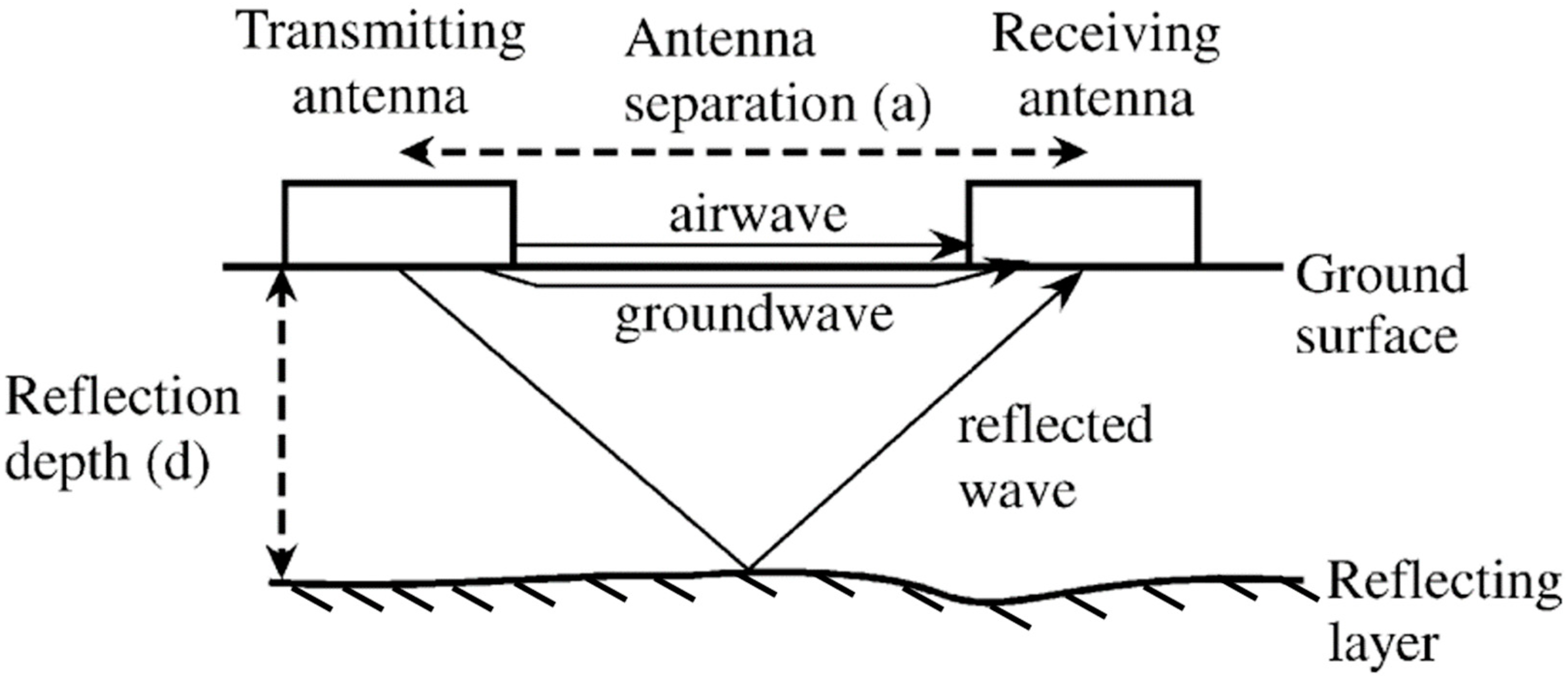
GPR is a geophysical technique that uses electromagnetic energy with center frequencies generally between 100 and 2500 MHz to image the subsurface [29]. The GPR transmitting antenna emits an outward electromagnetic wave, and some of the electromagnetic wave passes directly from the transmitting antenna to the receiving antenna through the air. Some of the electromagnetic wave, known as the direct wave, propagates along the soil’s surface to the receiving antenna, and the remainder of the electromagnetic wave, known as the ground wave, passes through the surface to the underground media and is reflected back to the receiving antenna from different interfaces [30,31] (Figure 1). When the ground wave encounters materials with different dielectric permittivities, such as intrusive bodies in the soil, soil voids, and different SWCs in the soil layers, the amplitude, frequency, and phase of the GPR electromagnetic signals change; thus, scattering and reflection occurs. Subsequently, the receiving antenna receives various kinds of reflected waves. Based on the two-way travel time (TWTT), phase, amplitude, and other parameters of the GPR electromagnetic waves, the average propagation velocity of the electromagnetic waves in the medium can be determined, and we can then obtain the dielectric constant. Consequently, we can predict the SWC through the radio wave propagation velocity equation or via the fitted curve between soil permittivity and SWC [29,32].
GPR is a valuable tool for SWC studies because the water content of a soil has a significant effect on the relative soil dielectric permittivity. The dielectric permittivity is a complex function with real and imaginary components, and it is usually defined as , where j is imaginary (i.e., j2 = −1), and and are the real and imaginary parts of the dielectric permittivity, respectively [12,34]. The dielectric permittivity is a frequency-dependent vector called the complex dielectric permittivity due to both and being dependent on the frequency. The imaginary part of the dielectric permittivity is called the energy dissipation and is related to the conductivity of the medium. In the case of GPR measurements, which commonly have frequencies ranging from 100 MHz to 2 GHz, most soils do not show dielectric relaxation and low conductivity. According to [35], the contribution of to soil salinity cannot be neglected, especially for GPRs operating at low frequencies (<1000 MHz). However, is often smaller than in nonsaline soils; thus, the imaginary dielectric permittivity is often ignored, and the real dielectric permittivity is called the relative dielectric permittivity (the dielectric permittivity referred to below is the real dielectric permittivity). In a composite material such as soil composed of water, air and minerals, the soil dielectric permittivity is determined by the relative contributions of the components. Because the dielectric permittivities of minerals (ε ≈ 2–5) and air (ε ≈ 1) are less than that of liquid water (ε ≈ 81) at 20 °C [35,36], the soil dielectric permittivity is controlled by the presence of water in the soil.
2.2. Experimental Materials
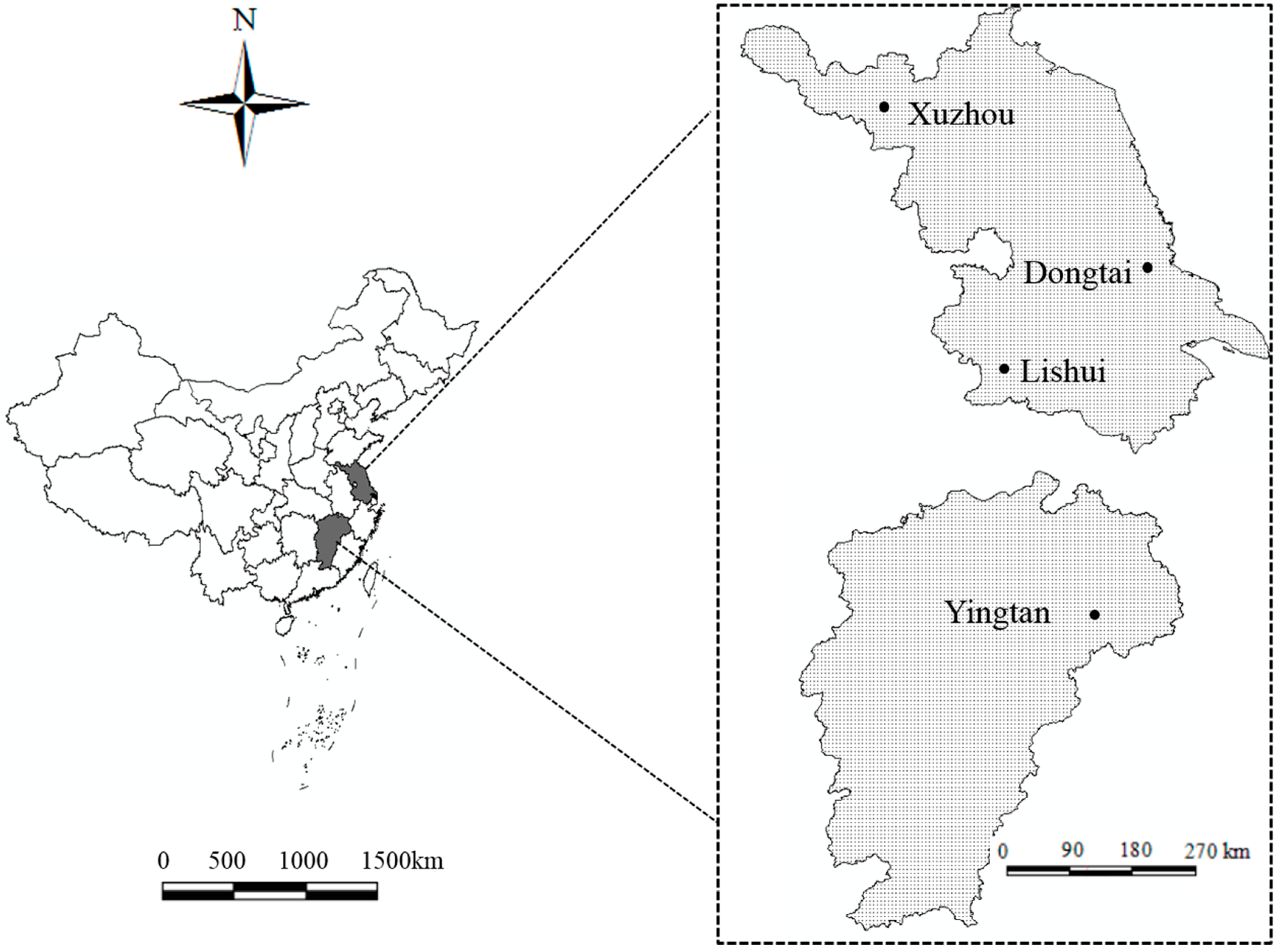
Experimental soils were collected from four regions: yellow brown soil (117°26′42″ E, 34°10′04″ N) and fluvo-aquic soil (116°29′43″ E, 34°43′37″ N) from Xuzhou, Jiangsu Province, China; brown soil (119°43′39″ E, 31°33′31″ N) from Lishui District, Nanjing, China; saline soil (120°33′42″ E, 32°45′58″ N) from Dongtai, Jiangsu Province, China; and red clay (116°58′42″ E, 28°28′06″ N) and red sandstone soil (116°52′26″ E, 28°07′33″ N) from Yingtan, Jiangxi Province, China (Figure 2). We collected 80 kg samples of each soil type from the surface layer (0–20 cm), and the basic soil physical and chemical properties, including soil pH, soil organic matter, soil bulk density, SWC, and soil texture, were measured according to [37]. Soil pH was measured in a 1:2.5 (w/v) ratio of soil to distilled water. Soil organic matter was determined using a KCr2O7-H2SO4 oil bath. SWC was measured by the gravimetric method, and soil bulk density was determined using the ring knives method. Soil texture was determined using a pipette and sieve analysis (Table 1). According to the USDA classification system, soil particles can be divided into three particle fractions based on size: clay (<0.002 mm), silt (0.002–0.05 mm), and sand (0.05–2.0 mm); except for the red clay and red sandstone soil, which are composed of clay and loamy sand, respectively, the soil textures of the soil types are silty loam. The tested soils were all naturally air-dried and sieved by a 2–7 mm mesh.
2.3. Experimental Design
An experimental box constructed of strong plexiglass was designed. To ensure that the depth of the soil model box was consistent with the thickness of the shallow soil in the field, we considered several experimental factors, such as tillage thickness. The model box was designed to have a volume of 60 × 30 × 25.4 cm3 (length × width × depth). Eight identical small holes with diameters of 2 cm were made in the bottom of the box, and three identical small holes were made in the front and back sides (Figure 3). The purpose of the holes was to facilitate soil water absorption and/or water loss during the experiment.
A 10-mesh nylon was placed on the bottom of the box, and the soil was homogenously backfilled into the box to reach the field-measured soil compaction. The thickness of the soil in the box was the same as the depth of the model box. To accurately extract the electromagnetic wave spectrum characteristics and the thickness of the reflected layer, reflectors A and B, each of which was 5.4 cm in diameter and 10 cm long, were buried at two positions in the model box. Reflector B was located on the bottom along the center axis, 15 cm from the left wall of the box. Reflector A was located 15 cm from the right wall of the box, and its top was 10 cm from the soil surface (Figure 3).
The soil characteristics, such as the SWC, soil bulk density, and weight of the dry soil, were measured and calculated in the GPR soil laboratory. The initial SWC of the filled soils was determined by the gravimetric method, and the box was then placed into a large water tank, allowing the soil to fully absorb water to reach a nearly saturated state. Subsequently, the box was placed in a cool dry place, and the soil was subjected to natural evaporation and air drying. GPR detection was performed once per day.
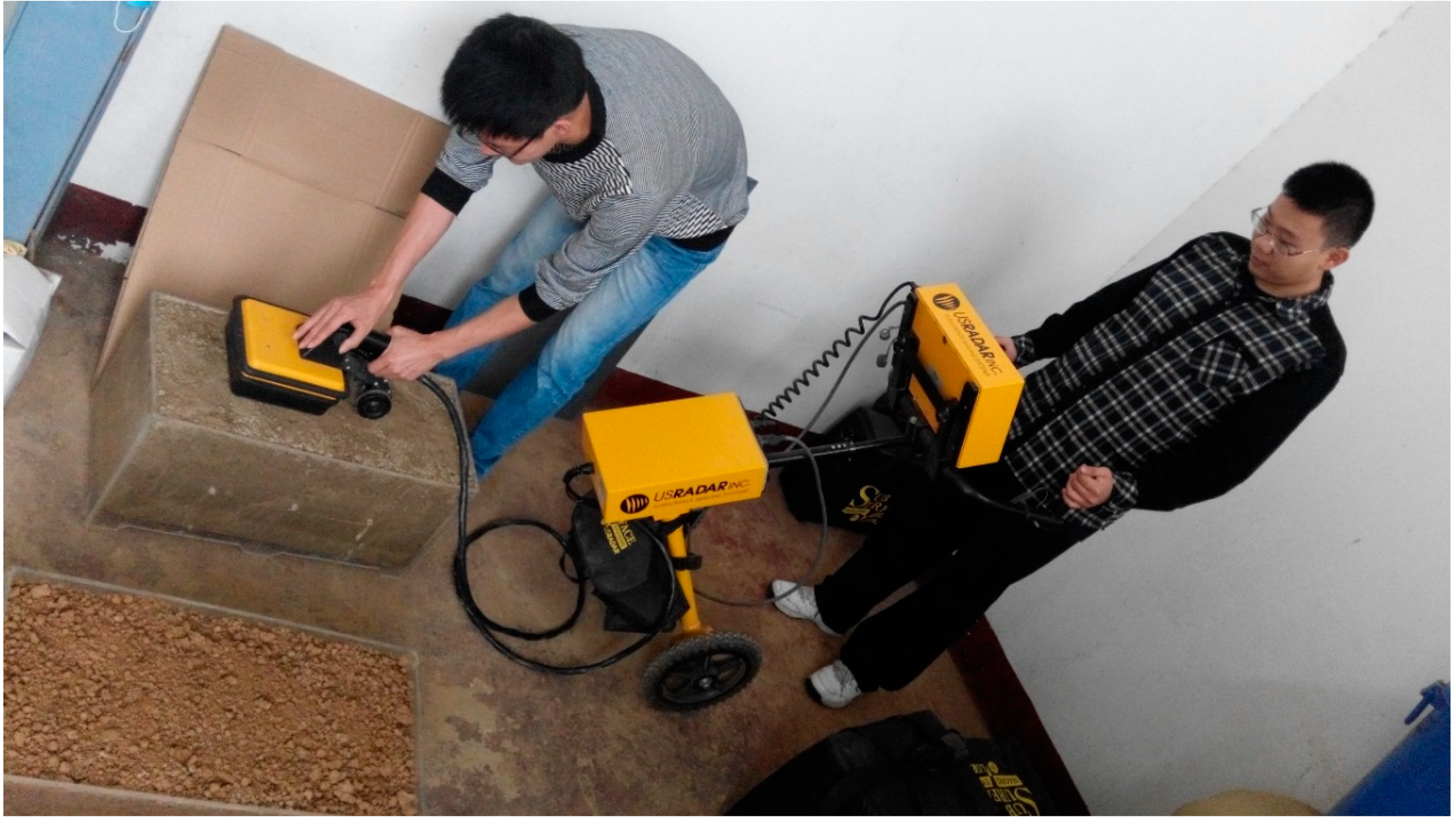
The GPR data acquisition system used in this study is the Seeker SPR GPR system, which is produced by US Radar and British ERA, and the process was performed using a shielded antenna with a frequency of 2 GHz. The GPR acquisition parameters are shown in Table 2. The interval of 0.005 m indicates that radar wave information is collected every 0.005 m, and the time window of 13 ns means that the time set on the longitudinal section is 13 ns, which determines the depth of detection. Depth indicates the maximum data acquisition depth of 0.4 m. The GPR’s shielded antenna was moved slowly along the soil surface of the model box, and the system automatically recorded and stored the data, repeating each probe three times (Figure 4).
We used the Reflexw 6.0 software (Earth Products China Ltd., Nanjing, China) to process the original GPR image data to facilitate the interpretation of the images and extract the parameters.
2.4. GPR Key Parameter Acquisition
(1) Two-way travel time
When performing GPR detection, the time required for the transmitting antenna’s emitted electromagnetic wave to reach a point in the medium and return to the receiving antenna can be directly determined from the GPR waveform image, and this time is defined as the TWTT [33] (Figure 5). The electromagnetic wave’s TWTT and the depths of the reflectors at the known locations were used to calculate the average soil dielectric permittivities above the reflectors.
(2) Electromagnetic wave velocity and soil dielectric permittivity
The electromagnetic waves emitted by an antenna-transmitter enter the soil and return after being reflected. The velocity of the waves is mainly affected by the soil dielectric permittivity (ε), magnetic permeability (μ), and electrical conductivity (δ) [27]:
where is the attenuation factor, (rad s−1) is the angular frequency, is the propagation velocity in a vacuum (3 × 10⁸ m s−1), and ε is the soil dielectric permittivity.
For materials with a low attenuation factor, such as sandy soil and low-saline soil, the influence of the electrical conductivity on the GPR frequency range is minimal and can thus be ignored. Therefore, ≈ 0. For most soils, the influence of the magnetic permeability on electromagnetic propagation is neglected; thus, μ ≈ 1 [35]. Consequently, Equation (4) can be simplified to the following:
In the case where the depth of the subsurface reflective medium is known, the average velocity of the GPR electromagnetic wave can be obtained by [38]:
where v is the GPR electromagnetic wave velocity (m ns−1), h is the depth of the underground target media (m), and TWTT is the two-way travel time of the GPR electromagnetic wave.
Therefore, ε can be obtained as follows:
3. Results
3.1. GPR Reflected Wave Image Features
Taking the red sandstone soil as an example, the x-axis represents the distance traveled by the GPR shield antenna, and the y-axis represents the TWTT of the radar wave (Figure 5). The GPR electromagnetic waves propagate in the soil, encounter reflectors A and B (the dielectric permittivity of the reflectors is different from the soil dielectric permittivity), and the radar spectrum characteristics change and show hyperbolic shapes (Figure 5). The hyperbolic characteristics diminish with increasing depth. After the first hyperbola of the radar wave signal, multiple echo oscillations are observed, which gradually decrease with increasing depth. The echo oscillations for reflector A are significantly stronger than those for reflector B because the radar waves are greatly attenuated with increasing depth, and reflector B is deeper; thus, the signal is weaker, and the echo characteristics are smaller. Although the overall characteristics are similar, a slight but visible difference between each plot can be noted; the TWTT increases with increasing SWC at the same location (Figure 5); thus, the returning signal from the bottom is delayed at a higher SWC because of the slower propagation of electromagnetic waves in the medium. The average soil dielectric permittivity above the reflector is calculated from the TWTT using Equation (4). Overall, the fundamental features in the GPR reflected wave image are identifiable and allow for proper validation of the synthetic setup, as discussed below. Processing the experimental GPR output is also possible; for example, the spectral content of the gathered GPR reflected wave image features can be derived by standard Fourier transform procedures.
3.2. Effect of SWC on GPR Electromagnetic Properties
The GPR TWTTs from reflectors A and B are important parameters of the GPR-reflected signals. The TWTT can be identified according to the location of the hyperbola from the reflector, the electromagnetic wave propagation velocity, and the depth of the underground layer. The TWTTs of the GPR electromagnetic waves at reflectors A and B have different values for the six soil types with different SWCs. The TWTTs of reflectors A and B increase gradually with increasing SWC (Table 3). Based on the identified TWTTs of reflectors A and B and Equations (3) and (4), we can calculate the average electromagnetic wave velocities VA and VB and then calculate the average soil dielectric permittivities above the reflectors (Table 3). As the TWTT increases, and the electromagnetic wave attenuation becomes more severe, fewer electromagnetic wave signals can reach the receiving antenna with increasing SWC at the same depth. Increasing the SWC directly affects the relative soil dielectric permittivity, the wave propagation velocity, and the GPR signal.
3.3. Retrieving SWC from the Soil Dielectric Permittivities
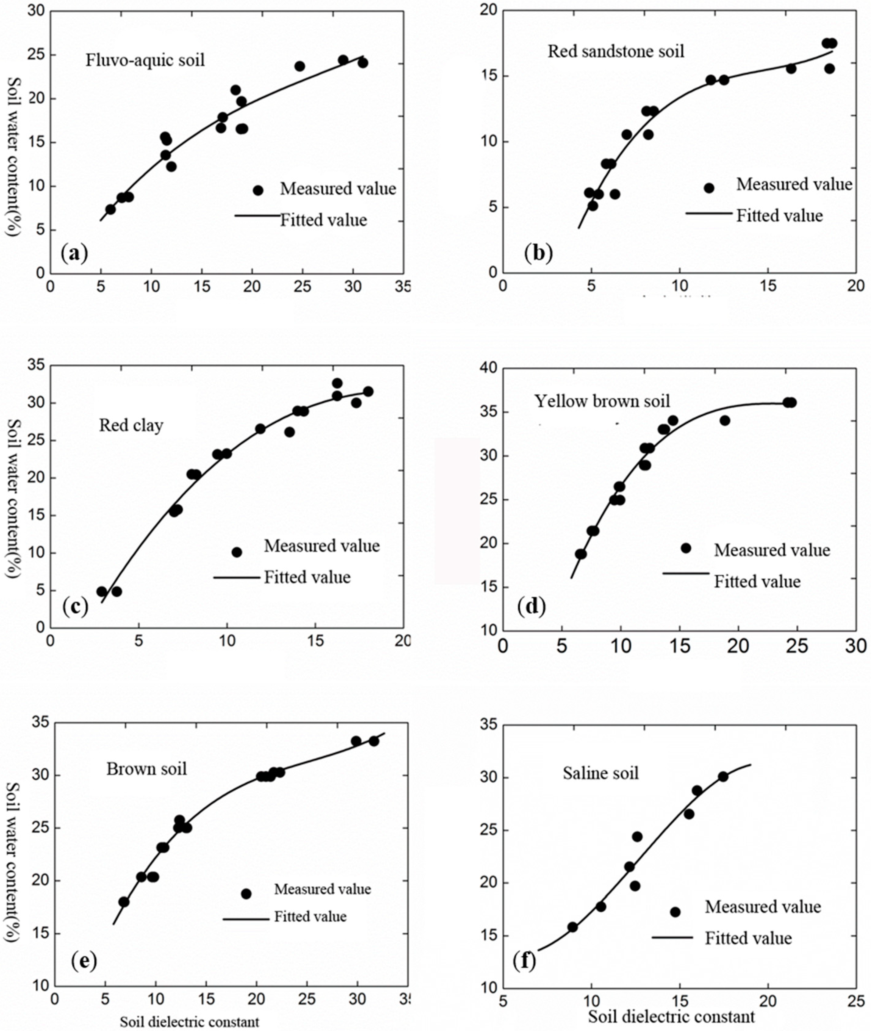
As shown in Figure 6, the soil dielectric constant increases continuously with increasing SWC. After the soil moisture reaches a certain value, the rate of increase in the soil dielectric constant becomes larger; i.e., a small change in the SWC can cause the soil dielectric constant to change considerably. The dielectric constants are different in the various soil types at the same water content; there are significant differences in different soils. For the fluvo-aquic soil, as the SWC increases gradually from 5% to 23%, the soil dielectric permittivity increases. The soil dielectric permittivity increases rapidly at SWCs greater than 23%. For the red clay, at SWCs below 15%, the corresponding soil dielectric permittivity changes slowly.
Linear regressions were used to fit the SWC (θ) and soil permittivity (ε) in the different soil types based on the 2-GHz antenna data, and the results are shown in Table 4. The fitted equations are all cubic polynomial models, and the correlation coefficients are greater than 0.9. However, the parameters of the cubic polynomial models are different in the different soil types. Therefore, it is necessary to calibrate the model parameters when using the model to determine SWC.
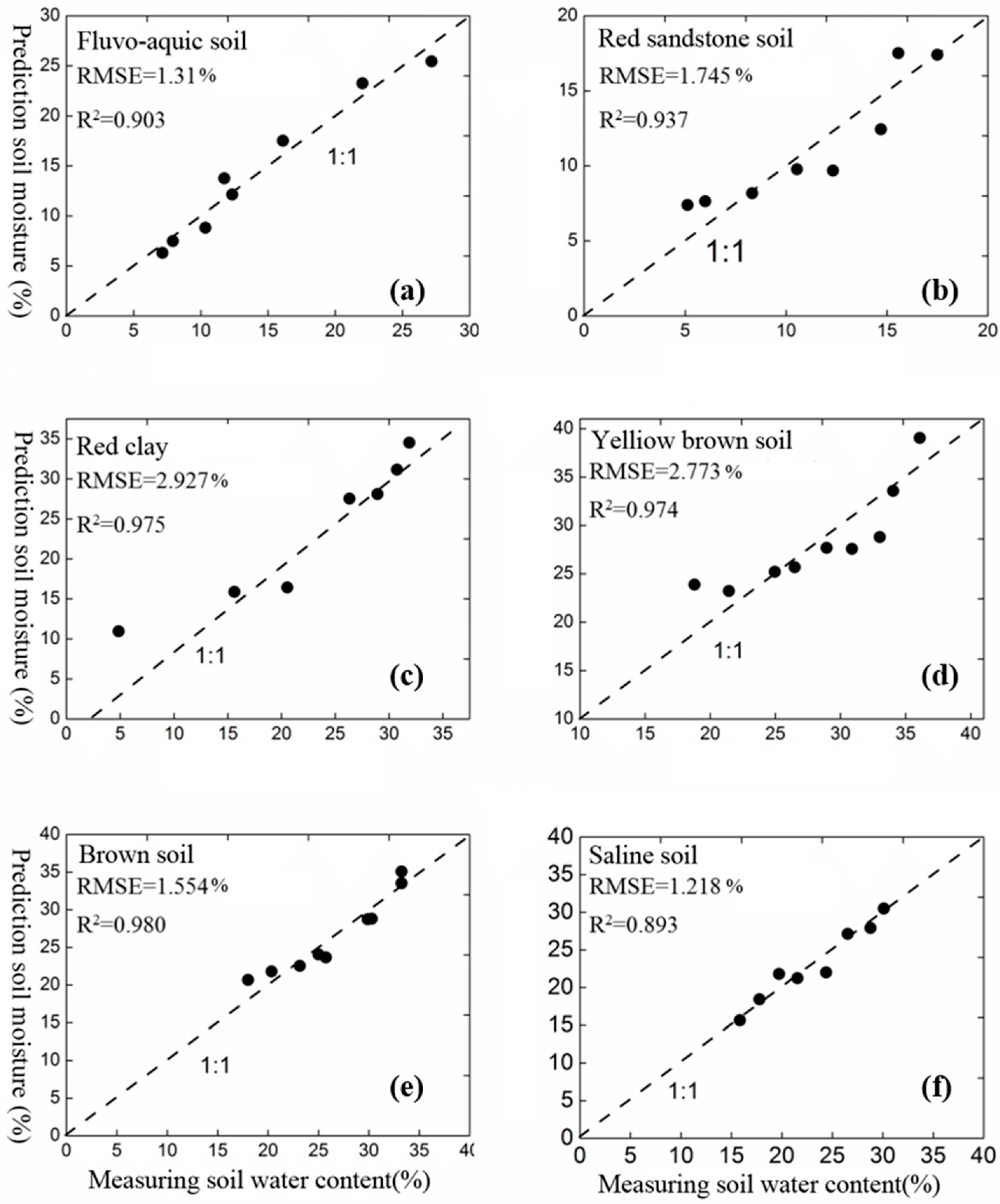
3.4. GPR-Derived SWC Validation
To determine the accuracy of the SWC retrieved with the 2-GHz GPR antenna, validation graphs are shown in Figure 7. The calculated and retrieved SWC values of the six soil types have relatively good correspondences. The RMSE of the red clay is the highest, and that of the saline soil is the lowest, with values of 2.92% and 1.22%, respectively. For the six soil types, the plots of the measured SWC values and the θ ~ ε model are close to the 1:1 line, and only a few values, such as those for the red clay and yellow brown soil, have slightly larger errors. A high-frequency GPR was successfully applied by [13] when determining SWC. The retrieved soil moisture values of the θ ~ ε model and the TDR-measured values have higher precision; both were close to the 1:1 line, and the absolute error was less than 1.47%. According to [24], authors used a GPR with a central frequency of 500 MHz to determine the GPR electromagnetic wave velocity and SWC in the laboratory and in an outdoor experiment. The results suggested that the soil dielectric constant depends strongly on the SWC and that a significant correlation exists between the soil dielectric constant and SWC, with a correlation coefficient of 0.882.
4. Discussion
4.1. Approach Based on Signal Velocity Analysis
In this study, a laboratory investigation was conducted to evaluate the use of a high-frequency GPR antenna to determine the SWC in loamy sand, clay and silty loam. The soil dielectric permittivity was calculated from the electromagnetic wave velocity determined using the reflection’s TWTT and the known depth. A reflector can be either a natural object or an artefact placed at a known depth. Many researchers have used GPR and reflectors at known depths to determine the SWC. For example, pre-embedded reflectors at known depths were successfully used by [33] when using GPR radar reflection data to estimate SWC, and the results had an RMS error of 0.018 m3 m−3. Although this approach is more accurate and appears to be simple, using it in the field can be difficult because it requires the object to be buried without disturbing the surrounding ground or excavating a natural object. In addition, the groundwater table approach was successfully applied by [28] when mapping the SWC of podzols. However, this approach requires a material that is penetrable by electromagnetic waves and a reflecting boundary at a known depth. In addition, the groundwater table is not fixed as it fluctuates with time [28]. If a known reflecting boundary is missing, the “common midpoint method”, “wide-angle-reflection-and-refraction method” or their variations can be used to determine the electromagnetic signal velocity and to estimate the SWC [27]. If there are several reflectors, the SWC in a vertical profile can be estimated [27].
4.2. Effects of Soil Properties on the Soil Dielectric Permittivity
The soil dielectric permittivity is a complex parameter that depends on the physical, mechanical, and chemical properties of the soil. Because soil consists of solids, liquids, and gases, the soil dielectric permittivity is determined by the characteristics and proportions of each phase. The soil dielectric permittivity and the dry mass density of the soil are linearly correlated and indicated that the dielectric permittivity of dry soils depends strongly on their porosity and compaction [39]. However, the SWC appears to be the major factor affecting the soil dielectric permittivity because water has the highest real permittivity (close to 81). Because of the real permittivities of dry soils, which range from 2 to 7, soil dielectric permittivity measurements will be highly dependent on the moisture content. According to [8,34,40], authors investigated the sensitivity of the soil dielectric permittivity to soil type and SWC, and the results showed that the real and imaginary parts of the soil dielectric permittivity () increased with increasing SWC in sandy soils.
The main factors affecting the soil dielectric parameters include the dielectric permittivity, electrical conductivity, and magnetic permeability. The magnetic permeability is only considered in materials that contain ferromagnetic minerals, such as magnetite and hematite. In these materials, a higher permeability decreases the electromagnetic signal’s penetration. In other materials, its influence is negligible [41,42]. In saline soils, the magnetic permeability cannot be ignored due to the high salt content. As the salt content of the soil increased, the real part of the dielectric permittivity () remained nearly constant, and the imaginary part () decreased [35,43].
The content of clay also has a large influence on the soil dielectric permittivity, which increases with the soil clay content. As the clay content increased, both the real and imaginary parts of the relative soil permittivity increased [23,26]. The reasons for the low soil dielectric permittivity at high soil clay contents are the high volume expansion, high moisture absorption capacity, and high electrical conductivity, which result in high dielectric losses.
4.3. Impact of Soil Parameters on SWC Prediction
The experimental results for a range of soil types at different SWC levels were analyzed. However, the results shows that SWC is not the only factor contributing to the soil dielectric permittivity; it is also affected by the soil texture, soil organic matter, soil density, and soil temperature.
At different temperatures and pressures, the relative soil dielectric permittivity can be expressed as follows [40]:
where is the pressure in millimeters of mercury (760 mm is the pressure of 1 atm), and is the temperature in °C. Representative solid dielectric constants are between 2 and 10. From this equation, we calculated the variation in the dielectric permittivity of water at different temperatures; the corresponding dielectric permittivities of water at 5, 20, and 35 °C are 86.1, 80.4, and 75.5, respectively. Thus, as the temperature increases, the dielectric permittivity of water decreases because of the increase in the activation energy of water molecules.
Soil organic matter also affects the soil dielectric permittivity; the soil permeability increases and the water retention capacity decreases with the increasing of the soil organic matter. The apparent permittivity and moisture were measured by [12] in a humid tropical soil with organic fractions of 4% to 7%. The SWCs calculated using Topp’s empirical model were significantly underestimated compared with the actual field moisture contents, which may have been related to the roles of both bound water absorbed by soil particles and the soil organic matter in decreasing the dielectric constant of the tested soil.
4.4. Comparative Analysis of SWC Predicted by GPRs with Different Frequencies
In this study, a 2-GHz GPR antenna was used to measure the shallow SWC, and a quantitative relationship between the soil dielectric constant and SWC was determined. The R2 value of the fitted model is greater than 0.89, and the RMSE is less than 3%, which indicates that the cubic polynomial models have reliable detection accuracy and that high-frequency GPR technology is feasible for measuring shallow SWC. However, the coefficients of the cubic polynomial model differ in the different soil types, which suggests the need to correct the model’s coefficients before using it to measure SWC. According to [44], a GPR with a center frequency of 900 MHz was used to measure SWC in loam and sandy soil. They fitted a cubic model with the soil permittivity and soil moisture and validated its accuracy. They found that the RMSE was less than 5.48% of the SWC measured using TDR. The 50- and 100-MHz GPR antennas and TDR were used to monitor the SWC in sandy loam and sandy areas of the Huang-Huai-Hai Plain, China. Their results suggested that the 50-MHz GPR cannot interpret electromagnetic waves and that the 100-MHz GPR had no ground wave signal in sandy loam soil. However, the electromagnetic wave signal could be clearly interpreted in sand, and the average standard deviation between the GPR-estimated values and the TDR-measured values was 10% [45]. A 100-MHz GPR was successfully applied when determining the average moisture content of loam in a field profile at depths from 0.8 m to 1.3 m, and the RMSE value was only 18% of the TDR-measured SWC [33]. In detecting SWC, although high-frequency GPR antennas have a higher detection accuracy than low-frequency GPRs, the detection depth of high-frequency GPR is shallow; it has a smaller wavelength, which allows high-resolution subsurface characteristics to be observed. Furthermore, the higher-frequency signal is strongly attenuated, so the penetration depth is smaller.
5. Conclusions
A laboratory study was conducted to evaluate the use of a high-frequency GPR antenna to determine the soil dielectric permittivity and shallow SWC in loamy sand, clay, and silty loam. The results indicated that high-frequency GPR provides feasible and reliable estimates of shallow SWC. The high-frequency GPR estimation of shallow SWC has many advantages: it measures shallow SWC at the field scale or intermediate scale of hundreds of meters; it is in-situ, rapid, low-cost, and nondestructive; and it does not use a radioactive source, so it is harmless to people and the environment. Although the detection depth of the high-frequency GPR antenna is shallow, the resolution and the SWC detection accuracy are high. This technology bridges the gap between point measurements and remote sensing measurements of SWC.
The GPR method relies on the existence of a reflector at a known depth, and the interpretation methods require a sufficient and spatially continuous subsurface contrast in the dielectric permittivity; thus, selecting and verifying the origin and depth of the reflector requires careful attention. In addition, the physical relationship between the soil dielectric permittivity and SWC varies, which limits its broad application. Future work will focus on estimating SWC without a reflector at a known depth. Accurate knowledge of the surface dielectric permittivity is also useful for further determining the underlying soil properties, such as those in the root zone, from radar data.
Author Contributions
Conceptualization, L.Z. and D.Y.; Methodology, L.Z.; Software, L.Z.; Validation, D.Y., Z.W. and X.W.; Formal Analysis, L.Z.; Investigation, L.Z. and D.Y.; Resources, D.Y.; Z.W. and X.W.; Data Curation, D.Y.; Z.W. and X.W.; Writing-Original Draft Preparation, L.Z.; Writing-Review & Editing, L.Z.; Visualization, L.Z.; Supervision, D.Y.; Z.W. and X.D.W.; Project Administration, Z.W.; Funding Acquisition, Z.W.
Funding
This research was funded by National key research and development plan project (2016YFC0502403), the National Natural Science Foundation of China (No.51879281), the Open Research Funds of State Key Laboratory of Simulation and Regulation of Water Cycle in River Basin, China Institute of Water Resources and Hydropower Research (No. SKL2018CG04), the National Natural Science Foundations of China (41701327).
Acknowledgments
The help and guidance of Naijia Guo and Xiyang Wang in the experimental work is gratefully acknowledged.
Conflicts of Interest
The authors declare no conflict of interest.
References
- Moghadas, D.; Jadoon, K.Z.; Lambot, S.; Vanderborght, J.; Vereecken, H. Monitoring near surface soil moisture profiles during evaporation using off-ground zero-offset ground-penetrating radar. EGU Gen. Assem. 2012, 14, 11988. [Google Scholar]
- Klotzsche, A.; Jonard, F.; Looms, M.C.; van der Kruk, J.; Huisman, J.A. Measuring Soil Water Content with Ground Penetrating Radar: A Decade of Progress. Vadose Zone J. 2018, 17, 1–9. [Google Scholar] [CrossRef]
- Vereecken, H.; Schnepf, A.; Hopmans, J.W.; Javaux, M.; Or, D.; Roose, T.; Vanderborght, J.; Young, M.H.; Amelung, W.; Aitkenhead, M. Modeling Soil Processes: Review, Key Challenges, and New Perspectives. Vadose Zone J. 2016, 15, 1–57. [Google Scholar] [CrossRef]
- Huisman, J.A. Measuring soil water content with ground penetrating radar: A review. Vadose Zone J. 2003, 2, 476–491. [Google Scholar] [CrossRef]
- Algeo, J.; Dam, R.L.V.; Slater, L. Early-Time, GPR: A Method to Monitor Spatial Variations in Soil Water Content during Irrigation in Clay Soils. Vadose Zone J. 2016, 15, 1–9. [Google Scholar] [CrossRef]
- Benedetto, A.; Tosti, F.; Ortuani, B.; Giudici, M.; Mele, M. Mapping the spatial variation of soil moisture at the large scale using GPR for pavement applications. Near Surf. Geophys. 2015, 13, 269–278. [Google Scholar] [CrossRef]
- Luo, T.X.H.; Lai, W.W.L.; Chang, R.K.W.; Goodman, D. GPR imaging criteria. J. Appl. Geophys. 2019, 165, 37–48. [Google Scholar] [CrossRef]
- Shamir, O.; Goldshleger, N.; Basson, U.; Reshef, M. Laboratory Measurements of Subsurface Spatial Moisture Content by Ground-Penetrating Radar (GPR) Diffraction and Reflection Imaging of Agricultural Soils. Remote Sens. 2018, 10, 1667. [Google Scholar] [CrossRef]
- Ercoli, M.; Di Matteo, L.; Pauselli, C.; Mancinelli, P.; Frapiccini, S.; Talegalli, L.; Cannata, A. Integrated GPR and laboratory water content measures of sandy soils: From laboratory to field scale. Constr. Build. Mater. 2018, 159, 734–744. [Google Scholar] [CrossRef]
- Topp, G.C.; Davis, J.L.; Annan, A.P. Electromagnetic determination of soil water content: Measurements in coaxial transmission lines. Water Resour. Res. 1980, 16, 574–582. [Google Scholar] [CrossRef]
- Weitz, A.M.; Grauel, W.T.; Keller, M.; Veldkamp, E. Calibration of time domain reflectometry technique using undisturbed soil samples from humid tropical soils of volcanic origin. Water Resour. Res. 1997, 33, 1241–1249. [Google Scholar] [CrossRef] [Green Version]
- Dam, R.L.V. Calibration Functions for Estimating Soil Moisture from GPR Dielectric Constant Measurements. Commun. Soil Sci. Plant Anal. 2014, 45, 392–413. [Google Scholar]
- Huisman, J.A.; Sperl, C.; Bouten, W.; Verstraten, J.M. Soil water content measurements at different scales: Accuracy of time domain reflectometry and ground-penetrating radar. J. Hydrol. 2001, 245, 48–58. [Google Scholar] [CrossRef]
- Wang, L.; Qu, J.J. Satellite remote sensing applications for surface soil moisture monitoring: A review. Front. Earth Sci. China 2009, 3, 237–247. [Google Scholar] [CrossRef]
- Bauer-Marschallinger, B.; Freeman, V.; Cao, S.; Paulik, C.; Schaufler, S.; Stachl, T.; Modanesi, S.; Massari, C.; Ciabatta, L.; Brocca, L.; et al. Toward Global Soil Moisture Monitoring With Sentinel-1: Harnessing Assets and Overcoming Obstacles. IEEE Trans. Geosci. Remote Sens. 2019, 57, 520–539. [Google Scholar] [CrossRef]
- Zeng, X.; Shan, W.; Zhang, Y.; Wang, C. Soil water content retrieval based on Sentinel-1A and Landsat 8 image for Bei’an-Heihe Expressway. Chin. J. Eco-Agric. 2017, 25, 118–126. (In Chinese) [Google Scholar]
- Chanzy, A.; Tarussov, A.; Judge, A.; Bonn, F. Soil Water Content Determination Using a Digital Ground-Penetrating Radar. Soil Sci. Soc. Am. J. 1996, 60, 1318–1326. [Google Scholar] [CrossRef]
- Jackson, T.J.; Schmugge, J.; Engman, E.T. Remote sensing applications to hydrology: Soil moisture. Int. Assoc. Sci. Hydrol. Bull. 1996, 41, 517–530. [Google Scholar] [CrossRef]
- Zreda, M.; Desilets, D.; Ferre, T.P.A.; Scott, R.L. Measuring soil moisture content non-invasively at intermediate spatial scale using cosmic-ray neutrons. Geophys. Res. Lett. 2008, 35, 1–5. [Google Scholar] [CrossRef]
- Jiao, Q.; Liu, S.; Jin, R.; Du, F. Research and Application of Cosmic-ray Fast Neutron Method to Measure Soil Moisture in the Field. Adv. Earth Sci. 2013, 28, 1136–1143. [Google Scholar]
- Strati, V.; Albéri, M.; Anconelli, S.; Baldoncini, M.; Bittelli, M.; Bottardi, C.; Chiarelli, E.; Fabbri, B.; Guidi, V.; Raptis, K.; et al. Modelling Soil Water Content in a Tomato Field: Proximal Gamma Ray Spectroscopy and Soil–Crop System Models. Agriculture 2018, 8, 60. [Google Scholar] [CrossRef]
- Baldoncini, M.; Albéri, M.; Bottardi, C.; Chiarelli, E.; Raptis, K.G.C.; Strati, V.; Mantovani, F. Biomass water content effect on soil moisture assessment via proximal gamma-ray spectroscopy. Geoderma 2019, 335, 69–77. [Google Scholar] [CrossRef]
- Yochim, A.; Zytner, R.G.; Mcbean, E.A.; Endres, A.L. Estimating water content in an active landfill with the aid of GPR. Waste Manag. 2013, 33, 2015–2028. [Google Scholar] [CrossRef] [PubMed]
- Wang, P.; Hu, Z.; Zhao, Y.; Li, X. Experimental study of soil compaction effects on GPR signals. J. Appl. Geophys. 2016, 126, 128–137. [Google Scholar] [CrossRef]
- Zhou, L.G.; Yu, D.S.; Wang, X.Y.; Wang, X.H.; Zhang, H.D. Determination of top soil water content based on high-frequency ground penetrating radar. Acta Pedol. Sin. 2016, 53, 621–626. (In Chinese) [Google Scholar]
- Lu, Y.; Song, W.; Lu, J.; Wang, X.; Tan, Y. An Examination of Soil Moisture Estimation Using Ground Penetrating Radar in Desert Steppe. Water 2017, 9, 521. [Google Scholar] [CrossRef]
- Zajícová, K.; Chuman, T. Application of ground penetrating radar methods in soil studies: A review. Geoderma 2019, 343, 116–129. [Google Scholar] [CrossRef]
- Overmeeren, R.A.V.; Sariowan, S.V.; Gehrels, J.C. Ground penetrating radar for determining volumetric soil water content; results of comparative measurements at two test sites. J. Hydrol. 1997, 197, 316–338. [Google Scholar] [CrossRef]
- Rogers, M.; Leon, J.F.; Fisher, K.D.; Manning, S.W.; Sewell, D. Comparing Similar Ground-penetrating Radar Surveys Under Different Moisture Conditions at Kalavasos-Ayios Dhimitrios, Cyprus. Archaeol. Prospect. 2012, 19, 297–305. [Google Scholar] [CrossRef]
- Reynolds, J.M. An Introduction to Applied and Environmental Geophysics; John Wiley & Sons Inc.: Hoboken, NJ, USA, 2011. [Google Scholar]
- Daniels, D. Ground Penetrating Radar, 2nd ed.; Wiley Interscience: London, UK, 2004. [Google Scholar]
- Ardekani, M.R.M. Off-and on-ground GPR techniques for field-scale soil moisture mapping. Geoderma 2013, 200, 55–66. [Google Scholar] [CrossRef]
- Lunt, I.A.; Hubbard, S.S.; Rubin, Y. Soil moisture content estimation using ground-penetrating radar reflection data. J. Hydrol. 2005, 307, 254–269. [Google Scholar] [CrossRef]
- Mohamed, A.-M.O.; Paleologos, E.K. Chapter 16—Dielectric Permittivity and Moisture Content. In Fundamentals of Geoenvironmental Engineering; Mohamed, A.-M.O., Paleologos, E.K., Eds.; Butterworth-Heinemann: Oxford, UK, 2018; pp. 581–637. [Google Scholar]
- Scudiero, E.; Berti, A.; Teatini, P.; Morari, F. Simultaneous Monitoring of Soil Water Content and Salinity with a Low-Cost Capacitance-Resistance Probe. Sensors 2012, 12, 17588–17607. [Google Scholar] [CrossRef] [Green Version]
- Leandro, C.G.; Barboza, E.G.; Caron, F.; de Jesus, F.A.N. GPR trace analysis for coastal depositional environments of southern Brazil. J. Appl. Geophys. 2019, 162, 1–12. [Google Scholar] [CrossRef]
- Liu, S.; Zhang, W.; Wang, K.; Pan, F.; Yang, S.; Shu, S. Factors controlling accumulation of soil organic carbon along vegetation succession in a typical karst region in Southwest China. Sci. Total Environ. 2015, 521–522, 52–58. [Google Scholar] [CrossRef]
- Chiara, F.D.; Fontul, S.; Fortunato, E. GPR Laboratory Tests For Railways Materials Dielectric Properties Assessment. Remote Sens. 2014, 6, 9712–9728. [Google Scholar] [CrossRef] [Green Version]
- Salat, C.; Junge, A. Dielectric permittivity of fine-grained fractions of soil samples from eastern Spain at 200 MHz. Geophysics 2010, 75, J1–J9. [Google Scholar] [CrossRef]
- Mohamed, A.-M.O.; Paleologos, E.K. Chapter 14—Electrical Properties of Soils. In Fundamentals of Geoenvironmental Engineering; Mohamed, A.-M.O., Paleologos, E.K., Eds.; Butterworth-Heinemann: Oxford, UK, 2018; pp. 497–533. [Google Scholar]
- Lal, H.B.; Dar, N.; Kumar, A. Electrical and magnetic properties of Er2(WO4)3. J. Phys. C Solid State Phys. 1975, 8, 2745–2748. [Google Scholar] [CrossRef]
- Cassidy, N.J. Chapter 2—Electrical and Magnetic Properties of Rocks, Soils and Fluids. In Ground Penetrating Radar Theory and Applications; Jol, H.M., Ed.; Elsevier: Amsterdam, The Netherlands, 2009; pp. 41–72. [Google Scholar]
- Sevostianova, E.; Deb, S.; Serena, M.; VanLeeuwen, D.; Leinauer, B. Accuracy of two electromagnetic soil water content sensors in saline soils. Soil Sci. Soc. Am. J. 2015, 79, 1752–1759. [Google Scholar] [CrossRef]
- Wu, Y.; Cui, F.; Wang, L.; Chen, J.; Li, Y. Detecting moisture content of soil by transmission-type ground penetrating radar. Trans. Chin. Soc. Agric. Eng. 2014, 30, 125–131. (In Chinese) [Google Scholar]
- Ji, L.Q.; Zhu, A.N.; Zhang, J.B.; Xin, X.L.; Li, X.P. Determining Soil Water Content by Using Low-frequency Ground-penetrating Radar Ground Wave Techniques. Soils 2011, 43, 123–129. (In Chinese) [Google Scholar]
Figure 1.
Structure and working principle of ground penetrating radar (GPR). Modified from [33].
Figure 1.
Structure and working principle of ground penetrating radar (GPR). Modified from [33].

Figure 2.
Geographic setting of the study area in China.

Figure 3.
Structure of the artificial model box.

Figure 4.
GPR measurement in the laboratory box.

Figure 5.
GPR reflected wave image features for the red sandstone soil. Note: TWTT(A) and TWTT(B) represent the two-way travel times of reflectors A and B, respectively; the SWCs of (a–c) are 28.77%, 21.54%, and 15.83%, respectively. The survey directions of panels b and c are opposite to that of panel a.

Figure 6.
Fitted curves between the soil dielectric constant and SWC. (a) fluvo-aquic soil; (b) red sandstone soil; (c) red clay; (d) yellow brown soil; (e) brown soil; (f) saline soil.
Figure 6.
Fitted curves between the soil dielectric constant and SWC. (a) fluvo-aquic soil; (b) red sandstone soil; (c) red clay; (d) yellow brown soil; (e) brown soil; (f) saline soil.

Figure 7.
Regression analysis of the measured SWC and the θ ~ ε model-retrieved SWC. (a) fluvo-aquic soil; (b) red sandstone soil; (c) red clay; (d) yellow brown soil; (e) brown soil; (f) saline soil.
Figure 7.
Regression analysis of the measured SWC and the θ ~ ε model-retrieved SWC. (a) fluvo-aquic soil; (b) red sandstone soil; (c) red clay; (d) yellow brown soil; (e) brown soil; (f) saline soil.


Table 1.
Basic physicochemical properties of the tested soils.
| Test Item | Soil Types | |||||
|---|---|---|---|---|---|---|
| Saline Soil | Fluvo-Aquic Soil | Yellow Brown Soil | Brown Soil | Red Clay | Red Sandstone Soil | |
| pH | 7.26 ± 0.21 | 6.69 ± 0.19 | 5.46 ± 0.31 | 7.62 ± 0.22 | 5.40 ± 0.24 | 5.70 ± 0.34 |
| Organic matter (g kg−1) | 7.98 ± 0.32 | 14.52 ± 0.17 | 8.78 ± 0.26 | 17.59 ± 0.18 | 20.16 ± 0.25 | 9.80 ± 0.23 |
| Soil bulk density (g cm−3) | 1.25 ± 0.031 | 1.19 ± 0.040 | 1.39 ± 0.052 | 1.14 ± 0.044 | 1.13 ± 0.063 | 1.32 ± 0.064 |
| Salt content (%) | 0.03 ± 0.0021 | 0.006 ± 0.0023 | 0.008 ± 0.0012 | 0.01 ± 0.0020 | 0.20 ± 0.021 | 0.10 ± 0.030 |
| Sand (2~0.05 mm) (%) | 14.8 ± 0.71 | 15.9 ± 1.00 | 17.7 ± 0.90 | 26.20 ± 1.72 | 29.2 ± 1.63 | 81.60 ± 2.12 |
| Silt (0.05~0.002 mm) (%) | 79.50 ± 1.22 | 68.50 ± 2.31 | 55.80 ± 1.17 | 66.40 ± 2.14 | 29.00 ± 1.23 | 11.20 ± 0.48 |
| Clay (<0.002 mm) (%) | 5.70 ± 0.51 | 15.6 ± 1.23 | 26.50 ± 0.36 | 7.40 ± 0.37 | 41.80 ± 2.11 | 7.20 ± 0.37 |
Notes: Values are means ± standard deviation. Each soil type had 3 samples.
Table 2.
GPR parameters.
| Antenna Frequency | Material Type | Interval (m) | Time Window (ns) | Stacking Fold | Depth (m) |
|---|---|---|---|---|---|
| 2 GHz | Soil | 0.005 | 13 | 8 | 0.4 |
Table 3.
GPR electromagnetic wave two-way travel times (TWTTs) and average velocities with various soil water contents.
Table 3.
GPR electromagnetic wave two-way travel times (TWTTs) and average velocities with various soil water contents.
| Soil Type | SWC (%) | TWTT(A) ns | TWTT(B) ns | Velocity (108 m s−1) | Soil Dielectric Permittivity (ε) | ||
|---|---|---|---|---|---|---|---|
| Fluvo-aquic soil | 24.00 | 2.78 | 4.41 | 0.07 | 0.09 | 0.08 ± 0.003 | 17.39 ± 1.45 |
| 16.65 | 2.19 | 4.23 | 0.09 | 0.09 | 0.09 ± 0.004 | 10.79 ± 0.86 | |
| 8.35 | 2.02 | 3.92 | 0.10 | 0.10 | 0.10 ± 0.002 | 9.18 ± 0.81 | |
| Red sandstone soil | 17.49 | 2.44 | 5.12 | 0.08 | 0.08 | 0.08 ± 0.003 | 13.40 ± 1.14 |
| 10.03 | 2.31 | 4.31 | 0.09 | 0.09 | 0.09 ± 0.003 | 12.01 ± 1.08 | |
| 6.12 | 2.12 | 3.83 | 0.09 | 0.10 | 0.10 ± 0.004 | 10.11 ± 1.02 | |
| Red clay soil | 30.74 | 2.64 | 4.85 | 0.08 | 0.08 | 0.08 ± 0.002 | 15.68 ± 1.23 |
| 15.48 | 2.51 | 4.53 | 0.08 | 0.09 | 0.08 ± 0.002 | 14.18 ± 1.27 | |
| 4.85 | 1.45 | 3.01 | 0.14 | 0.13 | 0.14 ± 0.004 | 4.73 ± 0.57 | |
| Yellow brown soil | 36.00 | 3.12 | 6.43 | 0.06 | 0.06 | 0.06 ± 0.001 | 21.90 ± 1.89 |
| 28.00 | 2.80 | 5.26 | 0.07 | 0.08 | 0.07 ± 0.002 | 17.64 ± 1.72 | |
| 21.00 | 2.21 | 4.62 | 0.09 | 0.09 | 0.09 ± 0.003 | 10.99 ± 0.89 | |
| Brown soil | 25.74 | 2.81 | 5.82 | 0.07 | 0.07 | 0.07 ± 0.002 | 17.77 ± 1.49 |
| 20.34 | 2.08 | 4.12 | 0.10 | 0.10 | 0.10 ± 0.000 | 9.73 ± 0.79 | |
| 18.01 | 1.42 | 3.01 | 0.14 | 0.13 | 0.14 ± 0.004 | 4.54 ± 0.37 | |
| Saline soil | 28.77 | 3.08 | 6.02 | 0.06 | 0.07 | 0.07 ± 0.002 | 21.34 ± 1.68 |
| 21.54 | 2.68 | 3.58 | 0.07 | 0.11 | 0.09 ± 0.003 | 16.16 ± 1.27 | |
| 15.83 | 2.00 | 4.08 | 0.10 | 0.10 | 0.10 ± 0.003 | 9.00 ± 0.71 | |
Note: TWTT(A) and TWTT(B) are the GPR reflection two-way travel times at reflectors A and B, respectively, which are recognized from the GPR spectrum; VA and VB are the average velocities above reflectors A and B, respectively, which are calculated by Equation (3); and ε is the average soil dielectric permittivity above reflector B, which is calculated by Equation (4).
Table 4.
Fitting curves between the dielectric constant and SWC for different soil types.
| Soil Types | Soil Texture | Curve Fitting | R2 |
|---|---|---|---|
| Fluvo-aquic soil | Silty loam | 0.90 | |
| Red sandstone soil | Loamy sand | 0.93 | |
| Red clay | Clay | 0.97 | |
| Yellow brown soil | Silty loam | 0.97 | |
| Brown soil | Silty loam | 0.98 | |
| Saline soil | Silty loam | 0.89 |
© 2019 by the authors. Licensee MDPI, Basel, Switzerland. This article is an open access article distributed under the terms and conditions of the Creative Commons Attribution (CC BY) license (http://creativecommons.org/licenses/by/4.0/).
Share and Cite
MDPI and ACS Style
Zhou, L.; Yu, D.; Wang, Z.; Wang, X. Soil Water Content Estimation Using High-Frequency Ground Penetrating Radar. Water 2019, 11, 1036. https://doi.org/10.3390/w11051036
AMA Style
Zhou L, Yu D, Wang Z, Wang X. Soil Water Content Estimation Using High-Frequency Ground Penetrating Radar. Water. 2019; 11(5):1036. https://doi.org/10.3390/w11051036
Chicago/Turabian StyleZhou, Ligang, Dongsheng Yu, Zhaoyan Wang, and Xiangdong Wang. 2019. "Soil Water Content Estimation Using High-Frequency Ground Penetrating Radar" Water 11, no. 5: 1036. https://doi.org/10.3390/w11051036
Note that from the first issue of 2016, this journal uses article numbers instead of page numbers. See further details here.