Extreme Precipitation Spatial Analog: In Search of an Alternative Approach for Future Extreme Precipitation in Urban Hydrological Studies


1
Department of Civil and Environmental Engineering, University of Illinois at Urbana-Champaign, Urbana, IL 61801, USA
2
Department of Atmospheric Sciences, University of Illinois at Urbana-Champaign, Urbana, IL 61801, USA
*
Author to whom correspondence should be addressed.
Water 2019, 11(5), 1032; https://doi.org/10.3390/w11051032
Submission received: 20 March 2019
/
Revised: 30 April 2019
/
Accepted: 10 May 2019
/
Published: 17 May 2019
(This article belongs to the Special Issue Extreme Floods and Droughts under Future Climate Scenarios)
Abstract
:In this paper, extreme precipitation spatial analog is examined as an alternative method to adapt extreme precipitation projections for use in urban hydrological studies. The idea for this method is that real climate records from some cities can serve as “analogs” that behave like potential future precipitation for other locations at small spatio-temporal scales. Extreme precipitation frequency quantiles of a 3.16 km catchment in the Chicago area, computed using simulations from North American Regional Climate Change Assessment Program (NARCCAP) Regional Climate Models (RCMs) with L-moment method, were compared to National Oceanic and Atmospheric Administration (NOAA) Atlas 14 (NA14) quantiles at other cities. Variances in raw NARCCAP historical quantiles from different combinations of RCMs, General Circulation Models (GCMs), and remapping methods are much larger than those in NA14. The performance for NARCCAP quantiles tend to depend more on the RCMs than the GCMs, especially at durations less than 24-h. The uncertainties in bias-corrected future quantiles of NARCCAP are still large compared to those of NA14, and increase with rainfall duration. Results show that future 3-h and 30-day rainfall in Chicago will be similar to historical rainfall from Memphis, TN and Springfield, IL, respectively. This indicates that the spatial analog is potentially useful, but highlights the fact that the analogs may depend on the duration of the rainfall of interest.
1. Introduction
The population in urban areas has increased by over 250% since 1964, and as a result, urban hydraulic infrastructure has dramatically increased [1,2]. Due to increased impervious surfaces, expanded coverage of storm sewers and other engineered drainage systems, and modified landscape, urban hydrologic systems have much smaller storage and shorter response time than the pre-development hydrologic systems. As a consequence, high-intensity short-duration precipitation extremes become one of the major causes of failures of hydraulic infrastructure in urban hydrologic systems [3], and thus play a significant part in studies and designs of urban hydraulic infrastructures. Design storms in particular, which are precipitation events of a specified duration and return period, are used universally in design of storm sewers [4], storage facilities [5], bridges and culverts [3], and in floodplain studies [6]. The return periods of these design storms can range from 2-year [4] to 100-year [5,6], while the durations range from less than an hour to several days depending on the purpose and scope of the structure being designed. The widely accepted and applied way to calculate design storms is to conduct frequency analysis on observed rainfall data with a stationarity assumption. However, as changes in extreme precipitation events have been observed [7] and are projected to continue [8] in a warmer climate by increasing studies, design storms analyzed using past data may not be applicable in the future [9]. Taking the state of Illinois as an example, flood damage on the order of billions of dollars was documented as a result from failures of urban hydraulic infrastructure under extreme rainfalls from 2007 to 2014 [4]. Urgent action is required in estimating future extreme rainfall to prevent losses and damages [10,11].
Even though extreme precipitation results from a combination of factors from large to local scales, global warming caused by anthropogenic greenhouse gases emission is likely to lead to the increase of precipitation extremes [8,12]. Atmospheric water holding capacity has increased [7,8] and is projected to increase in a warmer climate [8]. This increase in atmospheric humidity leads to increased frequency and intensity of the precipitation extremes, which are primarily controlled by variations in the atmosphere’s moisture content [7,8,13,14,15,16]. This is consistent with current observations and climate model simulations [7,8,17]. Kunkel [17] found that the frequencies of extreme precipitation events increased in the latter portion of the 20th century in the U.S., and the timing of this increase matched with a fast increase in global average temperatures. Trenberth et al. [7] showed that the precipitation extremes are in general observed to have an increasing trend, even though the magnitude varies with the location, duration, and frequency of the precipitation extremes.
General Circulation Models (GCMs) are the most recognized ways to project future precipitation patterns. However, the spatio-temporal resolution for these GCMs is usually very large: Most of the information is available at the daily time scale and 1 degree longitude and latitude (about several hundreds of kilometers) spatial scale, with cutting-edge GCMs towards sub-daily and 30 km spatio-temporal scales [18]. These GCM scales are much larger than the scales of urban catchments. Engineering remediation and design typically consider urban sewersheds or subcatchments less than 10 square kilometers. For example, the 960 sq km Chicago metropolitan area comprises about 218 sewersheds or subcatchments ranging from 0.05 to 23 sq km, with a median of 3 sq km [19,20]. Small catchments translate to a small time of concentration [20,21], which in turn requires means to estimate short duration, small time step (from several minutes to several hours) rainfall with both accurate volume and within-storm variability [22]. Therefore, downscaling methods are needed to communicate the information from GCMs to the requirements of civil engineering study & design.
Dynamical downscaling, a method that nests Regional Climate Models (RCMs) within GCMs to simulate regional climate behaviors, has become a widely accepted way to downscale GCM outputs for small scale climate change impact studies. To get good estimates of small scale precipitation intensity that can be used for urban hydrological and hydraulics (H & H) studies, it is important for RCM to run at small spatio-temporal resolutions, especially for precipitation extremes [15,23,24]. Gutowski et al. [25] pointed out that 15 km spatial resolution resulted in 6-h precipitation intensities that attain some acceptable precision in the RCM. Mishra et al. [16] suggested that resolution in the order of of 2–5 km might help in better capturing the statistics of 3-h precipitation extremes. However, existing RCM simulations with these small levels of spatio-temporal resolutions are specialized to either a short time domain or small spatial domain, due to high computational costs [8,26].
Large discrepancies may occur in the behavior of sub-daily extreme precipitation when the required resolutions are not met. Over North America, this generally results in underestimation of precipitation at coarser resolution [16,27,28]. The magnitude of underestimation increases as the rainfall duration decrease [16,27,28]. Mishra et al. [16] analyzed 3 and 24-h extreme precipitations at urban areas of the United States using the 50-km resolution North American Regional Climate Change Assessment Program (NARCCAP) [29] RCMs. Ninety-six of the 100 areas they studied have NARCCAP simulated 3-h 100-year return period precipitation underestimating the observations. Only a few of the locations were found to have RCM-simulated 3-h and 24-h 100-year return period extreme precipitation within the error band of the observed estimates.
In addition to the biases, small scale precipitation projections from dynamical downscaling may also be associated with large uncertainties. The driving GCM outputs are carrying uncertainties from emission scenario, GCM model formulation, and natural variability [27,30,31]. These uncertainties are amplified when added with uncertainties of RCM and RCM-GCM pairing in the downscaling process [31]. With better representation of changes in the small-scale processes, reducing the spatio-temporal resolution of RCM simulations can reduce the bias and also decrease the uncertainties in projected extreme precipitation [27]. Many studies have emphasized the importance of natural variability [32,33] and variations in RCM formulation [34] to the uncertainties of projected small-scale precipitation extremes. In recent years, extensive cross-agency efforts have been put into multi-model ensemble systems that compare different RCMs and realizations, like the NARCCAP program [29] and the Coordinated Regional Climate Downscaling Experiment (CORDEX) [35]. Multi-model ensemble systems with long-term simulations from different GCM-RCM should be able to account for uncertainties from natural variability, GCM and RCM model formulations, and GCM/RCM pairing. They are one of the most reliable data sources for future climate projections and are widely used in climate change impact studies [16,27].
Many previous studies have looked at accessing small-scale future precipitation extremes and the uncertainties associated with them. However, we need a better understanding of how different models project small-scale extreme precipitation at different frequencies and durations, as well as the uncertainties associated with these projections at different frequencies and durations. The first part of this study aims at answering these two questions. Simulated 3-h rainfall time series from NARCCAP were used in frequency analysis to estimate rainfall quantiles from 2-year to 100-year return period, at durations of 3-h, 24-h, and 30-day. The Calumet Drop Shaft-51 (CDS-51) catchment in the Chicago Metropolitan area was selected as a case study. Biases and uncertainties were analyzed at different frequencies and durations, from simulations of different NARCCAP GCM/RCM combinations.
Even though there are new data sources that use more updated emission scenarios, or smaller spatial steps that can better capture the behavior of small-scale extreme precipitation, those data sources are limited to selected model, time domain, and locations. NARCCAP is the dynamically downscaled multi-model ensemble for North America that has the smallest time step (3 h) and spatial step (50 km). However, there is still a gap between the spatio-temporal scales required for urban H & H studies, and the ones of available multi-model ensembles. When looking at short-duration extreme precipitation from NARCCAP, Mishra et al. [16] found that 3-h precipitation maxima means and 100-year return period magnitudes at a large number of studied urban areas across the United States are “largely underestimated” for both reanalysis and GCM boundary conditions, with biases over 10% of the observed estimates. These biases are not appropriate to use directly for stormwater infrastructure design purposes. They ascribed this bias to the weakness of RCMs in the convective parameterizations and its spatial scale.
One widespread interpretation for future climate change among both climatologists and end users is that “By the end of the century, an Illinois summer may well feel like one in East Texas today” [36]. An underlying assumption of this saying is that, the change of climate in time, from now to future, can be represented by the change of climate in space, from one place to another. Inspired by this idea, this paper examines an alternative method called extreme precipitation spatial analog to represent potential future extreme precipitation at small spatio-temporal scale. The spatial analog method uses real climate records from other locations to represent potential future climate. This is a novel alternative to the climate model projections and provides an intuitive way to communicate potential future climate projections to climate change adaptation and mitigation studies [29]. “A spatial analog is a location whose climate during a historical period is similar to the anticipated future climate at a reference location” [37]. As a “local, concrete, and immediate” [38] way to access future climate, the spatial analog method is particularly useful for urban studies, most of which focus on using multiple climate variables to study the social or economic vulnerability of cities [39,40,41,42]. Previous studies that looked at precipitation spatial analogs have focused on average precipitation patterns at large time scales. Hallegatte et al. [40], Grenier et al. [37], and Kellett et al. [42] used annual precipitation as the metric to find spatial analogs. Kopf et al. [41] include 30-year Aridity Index as a metric. Hallegatte et al. [40], Horváth et al. [43] and Ramírez-Villegas et al. [44] adopted monthly precipitation in their studies. Among rare attempts that studied precipitation spatial analog, Kellett et al. [42] looked at small temporal scale extreme precipitation of spatial analogs: Extreme daily precipitation of the whole study time periods were used as a metric for selecting spatial analogs. However, no previous study has focused only on looking at spatial analog for extreme precipitation, nor do they examine frequencies of sub-daily extreme precipitation in spatial analog. Extreme precipitation at sub-daily and shorter time scales have different mechanism to those at longer time scales [45]. The high variability of extreme precipitation at small spatio-temporal scales is crucial for urban hydrologic and hydraulic design. Existing studies mentioned the need for denser rain gauge network and finer resolution radar data [46,47]. However, due to their coarse resolution, current climate model ensemble projections are limited in their ability to represent small scale physics necessary to generate hydrologic data for urban H & H studies. The novelty of this approach is that it bridges the gap between projections from current climate model ensemble and fine spatial and temporal resolutions needed for H & H design by adopting the concept of spatial analog to extreme precipitation. When we borrowed the concept of spatial analog to focus only on extreme precipitation, the underlying hypothesis is that the future extreme storm characteristics of a certain location will be similar to the current extreme storm characteristics of a different location. Since extreme precipitation at different durations and frequencies are of interest for various urban H & H studies depending on their spatio-temporal scales, it is of great importance to study extreme precipitation spatial analog at different durations and frequencies.
In this study, we examine if an extreme precipitation spatial analog method is feasible to project future precipitation extremes at the scales required for urban H & H studies. Here we use the intensity-duration-frequency (IDF) relation as a metric for extreme rainfall spatial analog. The CDS-51 catchment in the Chicago Metropolitan area was selected as a case study to test the method. Given that current large model ensembles of climate model simulated dynamically downscaled rainfall have not yet reached the hourly and sub-hourly resolution, evaluating the possibility of using other cities’ high-resolution rainfall data to represent future precipitation of CDS-51 can be valuable for further climate change impact studies on urban H & H processes. Since CDS-51 is located in the Chicago metropolitan area of Illinois, this study can also evaluate the original concept of the transformation from temporal change to spatial change from Kling et al. [36], who used Illinois as an example to illustrate the migrating of climate.
Previous studies have showed that the intensity and duration of small duration heavy precipitation in the Chicago area are projected to increase [28,48,49]. Markus et al. [28] used rainfall outputs from one GCM and RCM combination with 30 km resolution to analyze the rainfall frequency quantiles for 2046–2055. Results showed that 24-h extreme precipitations of 2-year, 5-year, and 10-year return periods exhibited an average 20% and 16% increase under the Special Report on Emissions Scenarios (SRES) A1FI and B1 scenario [50] in the northern part, and a minor increase of 3% under A1FI scenario and a decrease of 12% under B1 scenario for the southeastern part. These results were updated by the same research group in 2018 [51], with projected increase in 24-h rainfall of 2-year to 100-year return period under SRES A1B, A2, and B1 scenarios using statistically downscaled 13 Coupled Model Intercomparison Project Phase 3 (CMIP3) models at 10 km resolution [52].
Dynamically downscaled model ensembles for North America using Coupled Model Intercomparison Project Phase 5 (CMIP5) data [53], like the North American Coordinated Regional Downscaling Experiment (NA-CORDEX) [54], do not have enough simulations from different RCM/GCM combinations at temporal scale as small as 3-h yet. Wuebbles et al. [55] have found that there are large variances between simulated extreme precipitation of different models in CMIP5 data. Extreme precipitation spatial analog derived using precipitation projections from only a few of CMIP5 models would be very uncertain. In addition, Wuebbles et al. [55] showed that the CMIP5 overall projected changes of extreme precipitation are in general similar to those of CMIP3 [56]. Specifically, Markus et al. [51] compared dynamically and statistically downscaling and also CMIP3 and CMIP5 projected daily extreme precipitation at the Chicago area and did not find significant difference. Taking all these factors into consideration, NARCCAP [29], which provide 3-h 50-km resolution rainfall simulations from over 10 combinations of RCM/GCM with SRES A2 scenario [50], is one of the best data sources for future extreme rainfall studies at the regional scale, and was used in this study to test the possibility of extreme precipitation spatial analog method. Future study can be conducted with more advanced multi-model ensembles to find extreme precipitation spatial analog using the method provided in this study.
2. Data and Methods
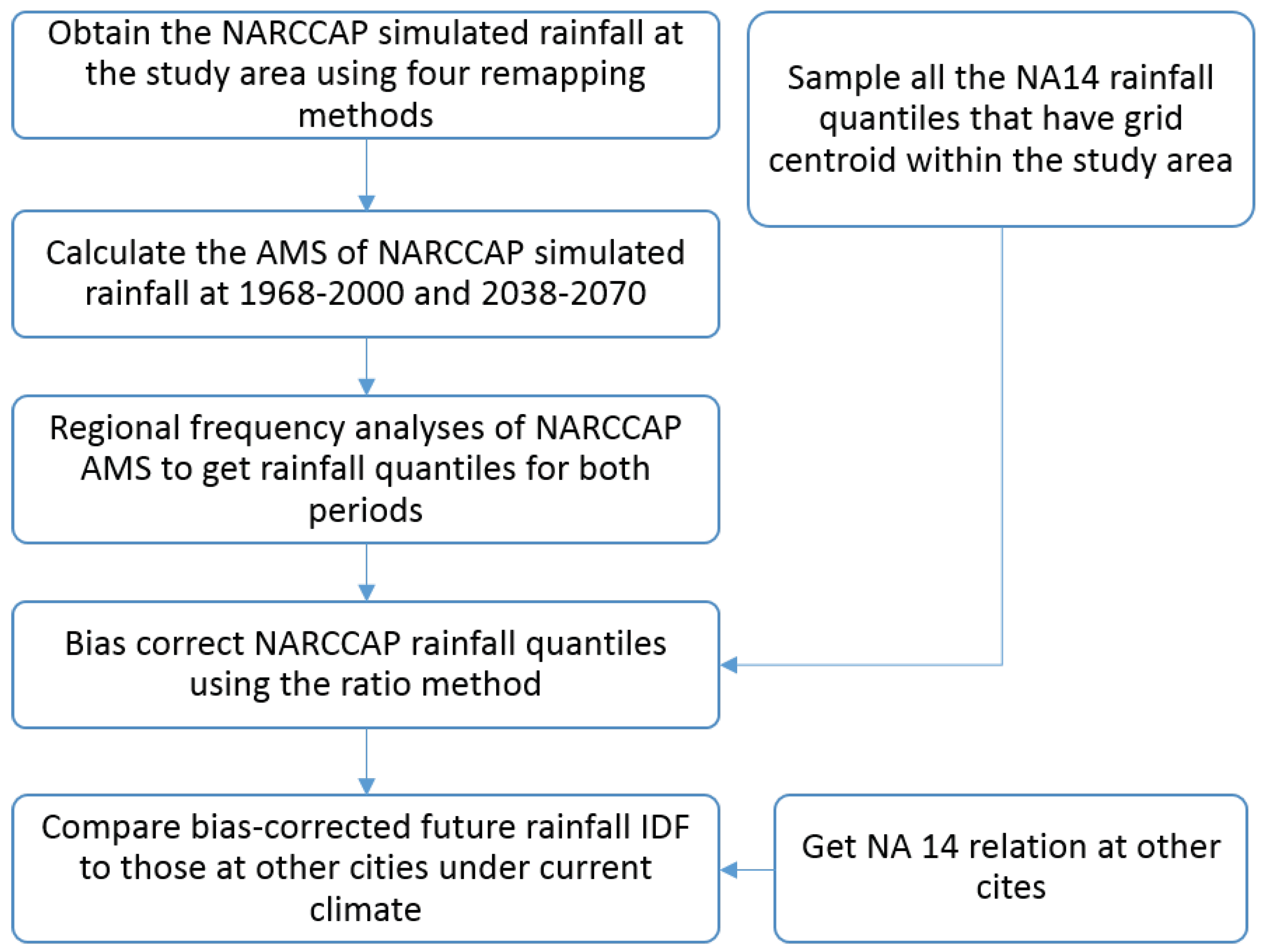
A schematic plot for the methodology of this study is shown in Figure 1. First we obtained the NARCCAP simulated rainfall data at the study area using four different remapping methods (see Section 2.1, Section 2.2 and Section 2.3). Then we calculated the annual maximum series (AMS) of NARCCAP rainfall at 1968–2000 and 2041–2070. Regional frequency analyses were conducted using these AMS to get frequency quantiles of NARCCAP rainfall data (see Section 2.4). We also sampled all the National Oceanic and Atmospheric Administration (NOAA) Atlas 14 (NA14) rainfall quantiles of the study area. After that, these NARCCAP rainfall frequency quantiles were bias-corrected with the ratio method using NA14 quantiles of the study area (see Section 2.5). Bias-corrected future NARCCAP rainfall quantiles were then compared to NA14 relations at other cites in search of potential spatial analog.
2.1. Study Site
The CDS-51 catchment (see Figure 2), which belongs to the Calumet system of Chicago’s Tunnel and Reservoir Plan (TARP) [57], has been widely used in H & H studies [20,58,59]. The CDS-51 catchment is a 5th-order complex urban system with an area of 3.16 km in the Village of Dolton, IL. The spatial characterization of the CDS-51 catchment was collected and analyzed during the Phase II of TARP project [20]. The critical duration for this catchment is 1 h [19].
2.2. Precipitation Data
The climate model simulated rainfall used in this study come from NARCCAP [29]. NARCCAP is an international program that aims at producing high resolution climate change simulations for investigating uncertainties in future climate projections and climate change study at regional scale for the North American region [29,60]. It provides dynamically downscaled precipitation at small spatial-temporal resolution of 50-km and 3-h, from different combinations of GCM and RCM. The 10 RCM/GCM combinations used in this study are shown in Table 1. The four GCM simulations were obtained from the CMIP3 archive [56]. The driving emission scenario for the GCM simulations is the SRES A2 scenario [50]. Under Phase II of NARCCAP, the five RCMs were run for the current period of 1968–2000 and future period of 2041–2070, with boundary conditions provided by those GCMs. Despite the fact that there are new GCM model simulations under updated climate models and emission scenarios, like the CMIP5 models and Representative Concentration Pathways (RCP) scenarios [18], in this study we chose the NARCCAP dataset with CMIP3 GCMs. As we argued previously, small spatial and temporal resolutions are needed for climate models to simulate the small-scale processes that are associated with urban catchment scale precipitation extremes. At the same time, to account for uncertainties and biases from model formulation and natural variability, multi-model ensemble is preferred to single model runs. Unfortunately, due to the large computation expense, dynamically downscaled small resolution multi-model ensembles using models from the CMIP5 archive under RCP emission scenarios are still not available for the entire United States. NARCCAP is the best dataset publicly available, dynamically downscaled to sub-daily time scale, verified and applied by many studies, and with a number of RCM/GCM combinations.
To evaluate the climate models’ performance, we compared the model simulated rainfall’s intensity-duration-frequency (IDF) relation under present-day climate with those of observations. The most recent nationwide calculation of rainfall quantiles, National Oceanic and Atmospheric Administration (NOAA) Atlas 14 (NA14) [61], was adopted in this study to represent the observed climate conditions. The NA14 rainfall data time periods are 1948–2000 for hourly rainfall measurements, and 1863–2000 for daily rainfall measurements. We looked at 3-h, 24-h, and 30-day precipitations from NA14. Rainfall quantiles with duration under 3-h were not used in this study, since NARCCAP cannot be used to provide rainfall quantiles at equivalent durations. Return periods examined are 2, 5, 10, 25, 50 and 100 years. IDF relations at the location of the study site and four cites south and west of Chicago (where the study site is located) were also obtained. The four cites are: Champaign IL, Springfield IL, St. Louis MO, and Memphis TN (see Figure 3). As can be seen in Figure 3, all five cities fall within 2.5 degree longitude of each other. Hence, we anticipate them to have similar climate. As locations shift south from Chicago to Memphis, we expected to see increases in precipitation extremes that could portray the changes in time projected for Chicago.
2.3. Regridding and Sampling of Rainfall Data
To account for the differences between spatial resolutions of NA14 precipitation dataset and NARCCAP simulated precipitation, the study area of this paper was set to be a rectangular grid centered at the centroid of CDS-51 catchment and has the same resolution of the NARCCAP horizontal grids (i.e., 50 km), which is shown as the area with the green boundary lines in Figure 2. This area is referred to as “the study area” or “the study grid”.
Different RCM/GCM combinations of NARCCAP have different horizontal grids systems even though they are in the same resolution. As a result, regridding or remapping is needed to interpolate horizontal fields of all model combinations to our study grid. Some research indicates that regridding might cause smoothing in the extremes [62,63], but it changes with a variety of factors including interpolation or averaging approach, number of points, etc. In this study, we quantified the potential uncertainties in regridding process by using four widely-recognized remapping methods: bilinear interpolation, bicubic interpolation, distance-weighted average remapping, and nearest neighbor remapping. The Climate Data Operators (CDO) [64] was used for the regridding process. Although we recognize the potential smoothing of extremes from regridding, we anticipate that the impact of smoothing is smaller than that of difference among different NARCCAP model grids, and therefore regridded the data to a consistent study grid. We include nearest-neighbor approach as this does not smooth the extremes.
As the study area is much larger than NA14 horizontal grids (0.0083 degrees longitude and latitude or around 900 m) [61], all NA14 grids that have their centroids inside the study area were obtained to provide the rainfall quantiles under present-day climate.
2.4. Precipitation Frequency Analysis and IDF Relation
Precipitation frequency analyses were conducted for NARCCAP simulations under historical and future periods using the L-moments method to get the IDF relations of rainfall. By picking the maximum rainfall depth of a certain duration for each year, AMS were formed for each of the selected durations. These AMS were then fitted into distributions using the L-moments method. The L-moments method [65] is widely used in precipitation frequency analyses, including the NA14 [61]. For this study, the L-moments are used instead of conventional moments, due to several reasons. First, L-moments “characterize a wider range of distributions”; second, when estimated from a sample, they are “more robust to the presence of outliers in the data”; third, L-moments are “less subject to bias in estimation” [65]. Details about the L-moments and frequency analysis using L-moments can be found in Hosking and Wallis [65]. In their book, Hosking and Wallis [65] defined L-moments as linear combinations of Probability Weighted Moments (PWM) . Greenwood et al. [66] defined the rth order PWM of a random variable X with cumulative distribution fuction to be . An unbiased estimator of given by Hosking and Wallis [65] is , where denotes the jth smallest value in a sample of size n. The relationship between PWM and popular L-moments are: L-location , L-scale , , . Popular L-moment ratios can be calculated by: L-CV , L-skewness , and L-kurtosis . The R package lmom [67] was used to conduct this analysis.
The purpose of this research is to explore the spatial analog method in extreme precipitation. The type of distribution that provides the best fit for extreme precipitation may be different among different models and durations, consequenctly the best fit frequency curve for each NARCCAP model precipitation series for each duration were selected from among five types of distributions: Generalized Logistic (GLO), Generalized Extreme Values (GEV), Generalized Normal (GNO), Generalized Pareto (GPA), and Pearson Type III (PE3) (see Table 2). Some studies recommend the GEV above other distributions for extreme precipitation frequency analysis [61,68,69]. But our comparison showed that the difference between two methods’ resulting quantiles are very small (on average −0.4%). The distributions with the smallest Root Mean Square Error (RMSE) were selected as the best fit distributions in this study [70,71,72]. Rainfall quantiles with the six different return periods selected for this study were then calculated using the quantile functions of the chosen distribution for each duration and RCM/GCM model combination.
Previous studies have mainly used two methods to extract extreme precipitation data for frequency analysis: Annual Maximum Series (AMS) and Partial Duration Series (PDS) [51,61]. AMS are formed by extracting the maximum values from each year of record. The PDS method, on the other hand, allows more than one extreme value to be extracted from a single year. The widely-adopted Chow et al. [73] method [51,61] (Equation (1)) was used to convert the return periods from NA14 data to the from the model projections. In this study, the we analyzed are 2, 5, 10, 25, 50, and 100 years. The corresponding were calculated using Equation (1), which were used later in frequency analysis of AMS to generate unbiased quantiles at our of interest. For example, when using Equation (1). This means that a 2-year unbiased quantile can be estimated by a 2.54-year AMS-based quantile.
2.5. Bias Correction
As discussed previously, climate model simulated precipitation can be biased. Correcting for biases in climate model output using historical data for future projections assumes that the past performance of climate model could be an indicator of future skill. Even though there are still debates on this issue, many studies have proved the existence of systematic errors in climate model outputs and showed some evidence supporting this assumption [51,74,75,76]. Bias correction was applied to NARCCAP future quantiles. The bias correction method used in the paper is the ratio method [28], also referred as the multiplicative change factor method [77]. The ratio method is a widely used linear correction method for extreme precipitation quantiles [28,78]. To get bias-corrected future quantile, , the ratio method multiplies the ratio between NA14 quantile O and model simulated quantiles of current climate P, to the model simulated quantiles of future period . In this study, this correction was conducted for every NARCCAP quantiles at each selected return period and duration, using all NA14 quantiles within the study area, as shown in Equation (2). All NARCCAP historical quantiles from different RCM, GCM, and grid-remapping methods, at different durations and return periods, were bias-corrected separately. Each of these NARCCAP historical quantiles were bias-corrected to all NA14 quantiles within the study grid. In this way, the spatial variations of NA14 quantiles at the scale of our study area are taken into the consideration by the bias-corrected future NARCCAP quantiles.
in which , is the bias-correction ratio, i stands for different durations, j stands for different return periods, k stands for the different NA14 grids within the study area, l stands for the different combinations of RCM, GCM, and remapping methods for NARCCAP quantiles.
3. Results
The results for frequency analysis are based on a grid centered at the CDS-51 catchment with the same horizontal resolution of a NARCCAP grid (50 km × 50 km). Rainfall frequency quantiles from NARCCAP simulations and NA14 were analyzed at rainfall durations of 3-h, 24-h, and 30-day.
3.1. Rainfall Frequency under Current Climate
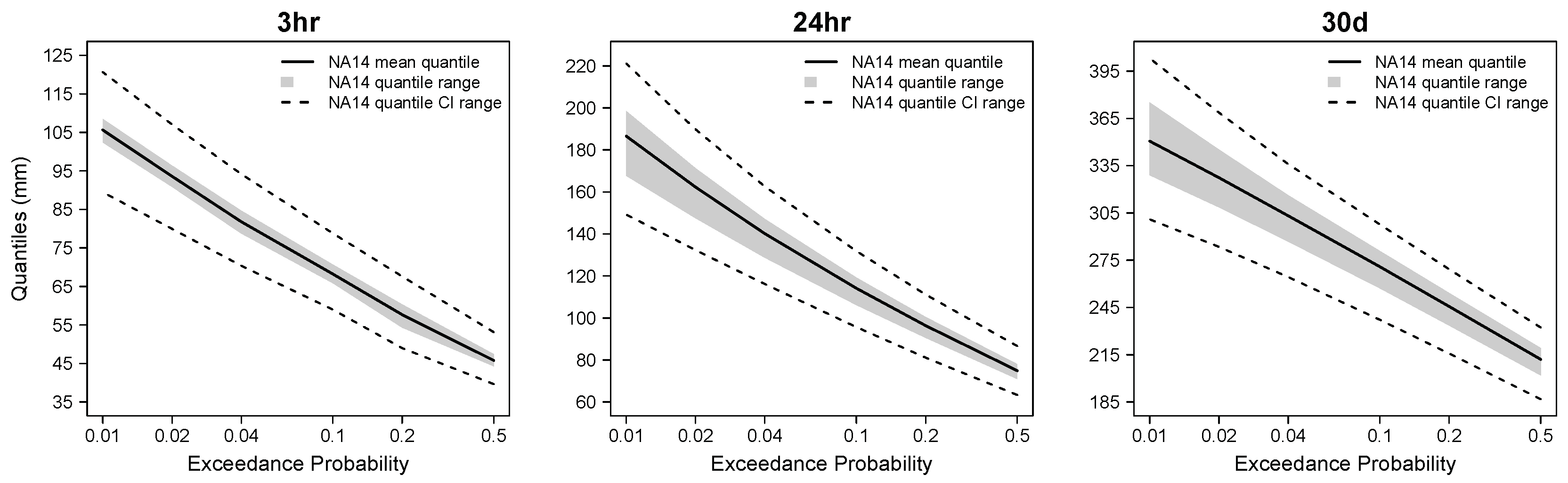
Figure 4 shows the rainfall frequency quantiles from NA14 of the study grid. The range of NA14 frequency quantile estimates within the study grid (the grey shaded area) reveals the spatial variance of rainfall statistics at the spatial resolution of NARCCAP data at CDS-51. At the 3-h rainfall duration, this spatial variance is much smaller than those at 24-h and 30-day durations. The spatial variance is also increasing with decreasing exceedance probability (or the increase of return period). This trend is more obvious in 24-h and 30-day rainfall than in 3-h rainfall. At 100-year return period, the spatial variance of NA14 quantiles can be as high as 20 mm for 24-h and over 30 mm for 30-day rainfall. In addition to the variance caused by the spatial scale of the study grid, the confidence intervals of the frequency quantiles also are increasing slightly with decreasing of exceedance probability.
3.2. Modeled Historical Period Rainfall Quantiles vs. Current Rainfall Quantiles
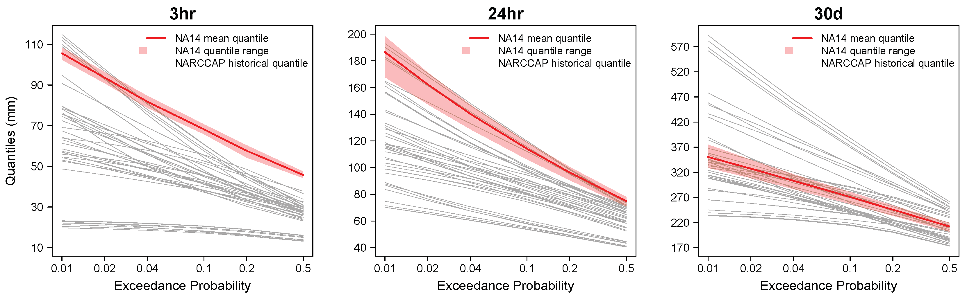
Figure 5 shows the comparison between frequency quantiles from NARCCAP simulations of historical periods (1968–2000) and NA14 for the study grid. There are 40 NARCCAP realizations in total, from 10 RCM/GCM combinations, each regridded using four remapping methods. The uncertainties that come from GCM, RCM, and grid remapping for the NARCCAP frequency quantiles are extremely large compared to the range of NA14 frequency quantiles within the study grid. These uncertainties increase at longer return periods. At the 3-h duration, most of the NARCCAP historical frequency quantiles underestimate the observed NA14 frequency quantiles, except for those with return periods larger than 50-year. For 24-h rainfall, the NA14 frequency quantiles generally lie at the upper bound of the NARCCAP historical quantiles range. Our results are comparable to the findings of Mishra et al. [16], that NARCCAP RCM underestimate 3-h and 24-h extreme precipitations in the east part of the United States. However, for the 30-day duration events, the NA14 quantiles are within the variability of the NARCCAP historical quantiles. The large uncertainty in the model-simulated rainfall quantiles is the motivation for using bias-correction. As will be discussed below, using bias-correction we are able to easily quantify changes to the different quantiles, despite the biases that may exist for individual model simulations.
3.3. Bias-Correction of Modeled Frequency Quantiles
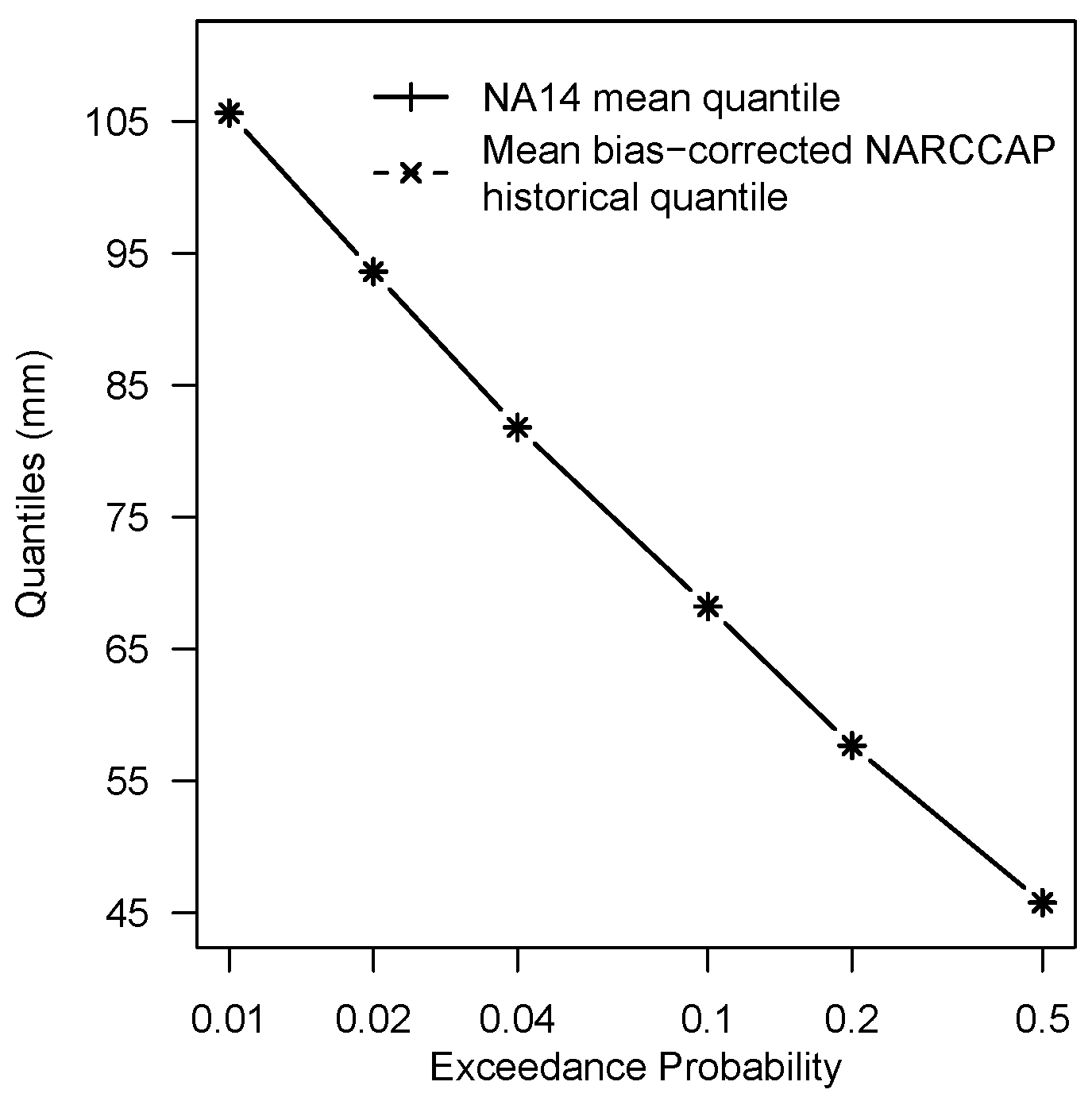
Bias-correction forces the frequency quantiles of NARCCAP historical time period to match the NA14 quantiles. By multiplying the ratio of each NA14 quantile within the study grid to each of the NARCCAP quantiles, all NARCCAP quantiles from different RCM/GCM combinations, remapping methods, at different return periods and durations, coincided with the specific NA14 quantile used for bias-correction. As shown as an example for 3-h rainfall in Figure 6, the mean of all bias-corrected NARCCAP historical quantiles coincide with the mean of NA14 quantiles at all exceedance probabilities. The mean bias-correction ratios for each GCM and RCM combination are shown in Figure 7. These ratios can serve as evaluations of the performance of RCM and GCM. Values larger than 1 indicate that the particular NARCCAP model is underestimating precipitation, while values less than 1 indicate overestimation. Some models perform better at smaller durations, while others better at longer durations. For example, HRM3 model frequency quantiles are the closest ones to NA14 quantiles at 3-h and 24-h durations, but for 30-day duration they tend to overestimate the NA14 quantiles. CCSM model results largely underestimate at 3-h and 24-h durations, but their results at 30-day duration are realistic. Models can also perform differently at different return periods. In addition, the correction ratios tend to depend more on the RCM than the GCMs: Cells with the same RCM have more similar colors than cells with the same GCM (Figure 7). This result matches with the finding of Monette et al. [79] and Khaliq et al. [80] who studied seasonal 1-day to 10-day extreme precipitations for Canadian watersheds using NARCCAP data. The control of RCM on the performance seems to gets weaker at 30-day duration, where ratios of the same RCM model can be very different from each other. Taking HRM3 again as an example, at 30-day duration, ratios of HRM3+gfdl have a relatively good performance, with more overestimation at larger exceedance probabilities, while ratios of HRM3+hadcm3 are giving the worst results among all the model combinations, with more overestimation at smaller exceedance probabilities. This overestimation of HRM3 was also observed by previous study of Monette et al. [79]. They found that HRM3 tends to overestimate multiday rainfall extremes, with more bias at longer duration and return period.
3.4. Bias-Corrected Modeled Future Frequency Quantiles
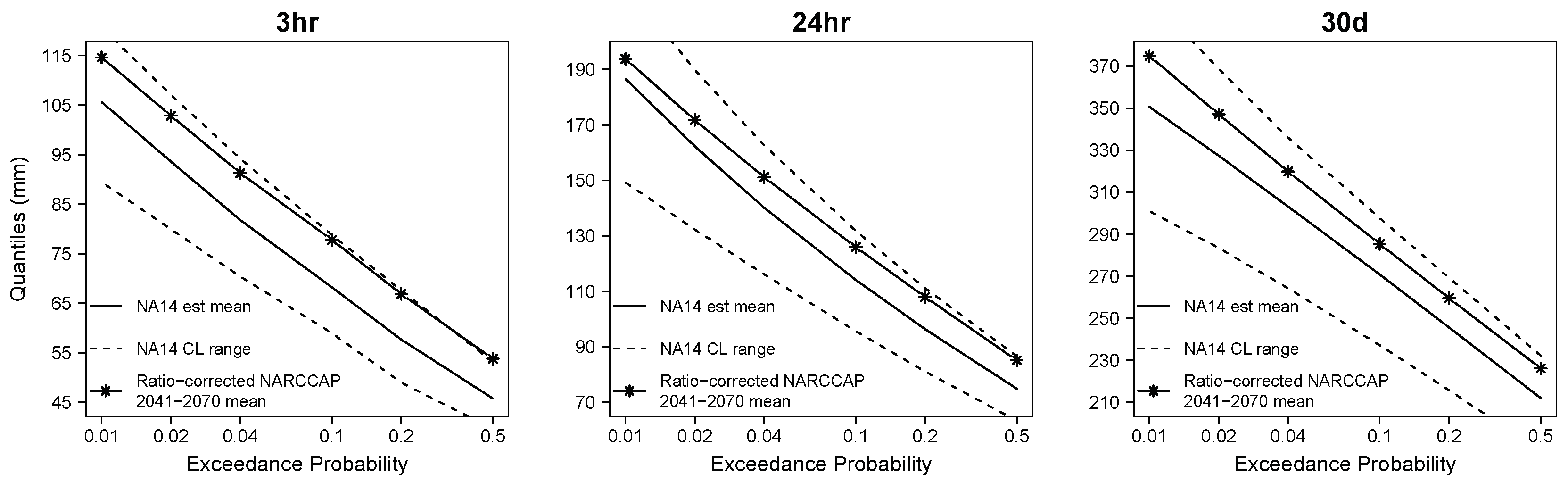
Figure 8 shows the average behavior of future bias-corrected NARCCAP frequency quantiles and NA14 frequency quantiles of the study area. There is a clear increase in rainfall depth in the bias-corrected future mean NARCCAP quantiles for all three durations from 3-h to 30-day, when compared to the NA14 quantiles. For 3-h rainfall, this increase of rainfall depth is almost an identical increase of about 8 mm at different exceedance probabilities from 0.01 to 0.5. At the 24-h duration, the difference between mean bias-corrected future quantiles and NA14 quantiles decreases for longer return periods. On the other hand, at the 30-day duration, this difference increases slightly at longer return periods, with a maximum difference of over 20 mm. Even though these differences between “current” and mean projected future frequency quantiles are obvious, they may not be statistical significant: Most of the bias-corrected NARCCAP future quantiles are still within the confidence intervals of the NA14 quantile range. The only exception is at 3-h duration and exceedance probability larger than 0.2. In general, at larger exceedance probabilities the mean bias-corrected future quantiles are closer to the upper boundary of confidence limits of the “current” frequency quantiles range of the study area.
A Welch Two Sample t-test analysis on the difference of the means and a Wilcoxon Rank-Sum test of the two-sample medians indicated that the means and medians of bias-corrected NARCCAP future (2041–2070) quantiles are different from NA14 quantiles of the study area at all analyzed exceedance probabilities and durations. Welch Two Sample t-test is an unpaired two-sample location test with a null hypothesis that the two populations have equal means. It assumes normality and is more reliable than Student t-test when the two samples have unequal variances. Wilcoxson Rank-Sum test is a non-parametric test with a null hypothesis that the two populations have equal median. It does not assume normality but does assume equal variance. By using both tests, we can perform robust statistical inference on the difference between average behaviors of the bias-corrected NARCCAP future quantiles and NA14 quantiles. The results from both tests indicate that the average projected future rainfall quantiles are larger than those under current climate for the study area with high confidence.
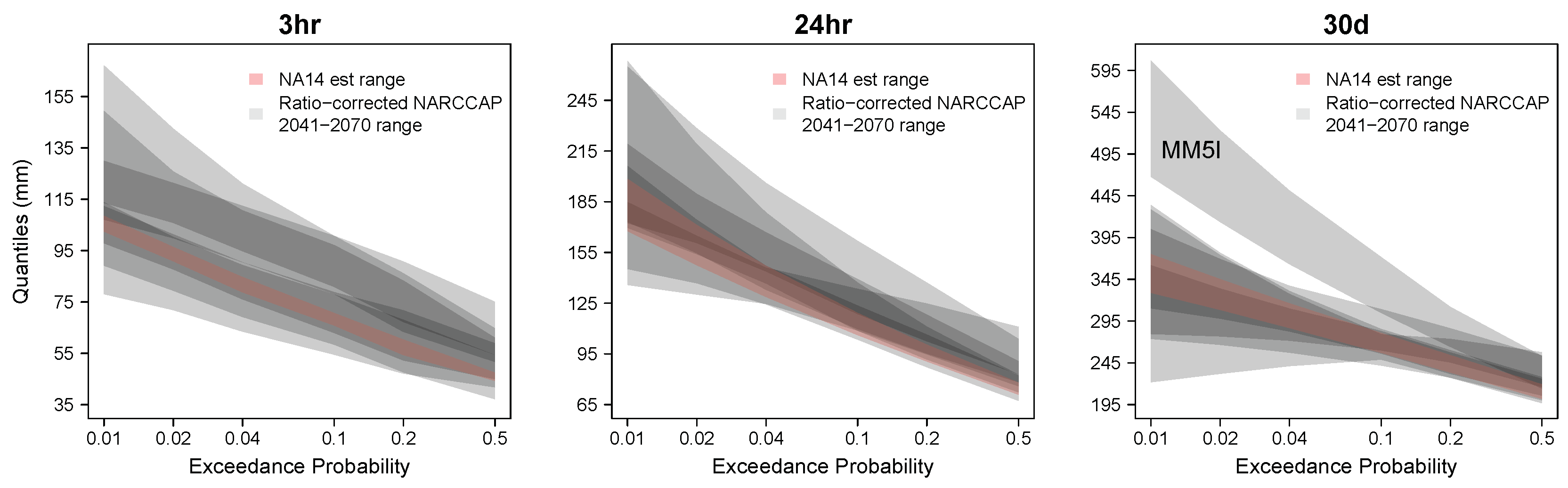
Figure 9 shows how the range of future bias-corrected NARCCAP frequency quantiles and NA14 frequency quantiles of the study area compare to each other. The range of bias-corrected NARCCAP future quantiles are always much larger than the NA14 quantiles. Furthermore, the NA14 ranges are within the NARCCAP ensemble for all three durations. The NA14 range increases with longer return periods and longer rainfall durations from 3-h to 30-day. Bias-corrected future NARCCAP ranges also increase for longer return periods and rainfall durations. Figure 9 also shows all the realizations of future bias-corrected NARCCAP quantiles compared to NA14 quantiles of the study area. The darkness of the grey color represents the density of future NARCCAP realizations. In general, NARCCAP bias-corrected future quantiles are higher than NA14 at all frequencies, especially at smaller durations of 3-h and 24-h. At the duration of 30-day, with the extreme high values of MM5I model at longer return periods, the mean future NARCCAP quantiles are higher than NA14 quantiles (as shown in Figure 8).
3.5. Rainfall Frequency Quantiles from Other Cities under Current Climate
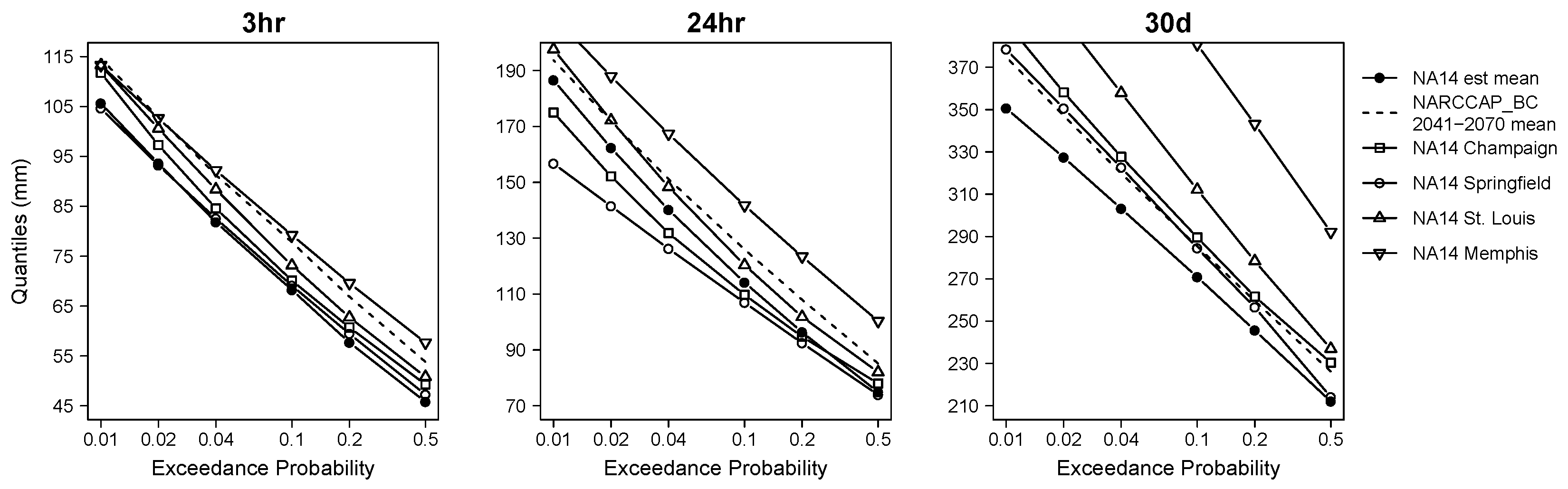
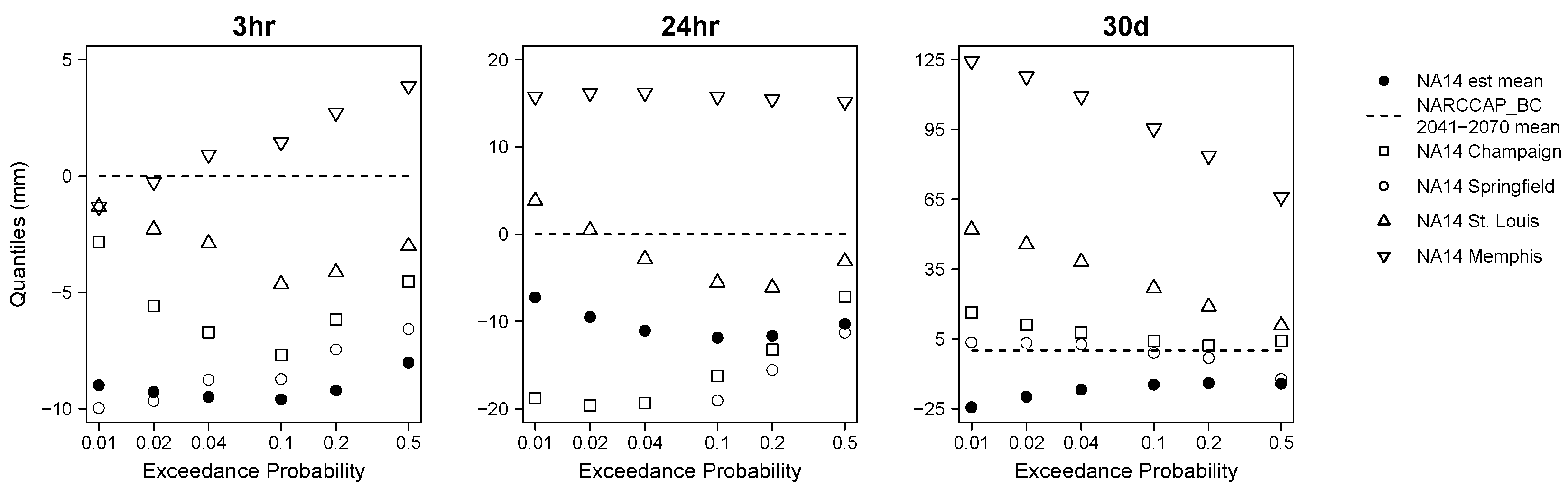
NA14 quantiles from several other cities south of Chicago were used to compare with the projected future changes in rainfall. Figure 10 shows how bias-corrected NARCCAP future frequency quantiles of the study area compare to the NA14 quantiles of those other cities south of the study area. Figure 11 shows the differences between the quantiles from NA14 and mean bias-corrected NARCCAP future quantiles. For 3-h rainfall, the NA14 quantiles from Memphis is the closest one to the mean bias-corrected NARCCAP future quantiles. At 24-h duration, NA14 quantiles from St. Louis are the nearest to NARCCAP bias-corrected future mean quantiles of the study area. For 30-day duration, NA14 quantiles from Springfield and Champaign are closest to NARCCAP bias-corrected future mean quantiles of the study area.
The result supports our hypothesis that the change of extreme precipitation in time, from now to future, can be approximated by the change of extreme precipitation in space, from one location to others. This implies that the spatial analog method is feasible to utilize observed precipitation data from one location to represent potential future extreme precipitation. For example, Memphis can be used as 3-h extreme precipitation spatial analog for the study area; St. Louis can be used as 24-h extreme precipitation spatial analog for the study area; Springfield and Champaign can be used as 30-day extreme precipitation spatial analog for the study area. Spatial analog of extreme precipitation will likely depend on the duration of rainfall of interest.
4. Conclusions and Discussion
It has been hypothesized that as climate warms, the temperature and precipitation in a location such as Illinois could be more like the climate in a more southern location like Texas [36]. This implies that we could potentially use spatial analogs, instead of relying on GCM projections of future climate. This is particularly attractive in the case of urban water infrastructure, because of the very small spatial and temporal scales required for the design of stormwater systems. We test the spatial analog hypothesis by analyzing the observed extreme precipitation, characterized using NA14 IDF relations, at 3-h, 24-h, and 30-day durations and 2-year to 100-year return periods, in a study grid that centered at Calumet Drop Shaft-51 catchment of the Chicago metropolitan area. We compare these observations with future projections of extreme precipitation as simulated using bias-corrected IDF relations from RCM-GCM combinations from the NARCCAP ensemble under SRES A2 scenario for the period 2041–2070. We then compare the NARCCAP projections with observed extreme precipitation in four other more southern cities: Champaign, Springfield, St. Louis, and Memphis. Although NARCCAP simulations are used in this study the analysis can be easily applied to updated RCMs as these data become more widely available.
The major findings of this study are:
- The variances in raw NARCCAP historical frequency quantiles from different combinations of RCM, GCM, and grid remapping methods are much larger than the variance of NA14 quantiles within the study area for all three durations analyzed. Most NARCCAP historical realizations tend to underestimate NA14 quantiles at smaller durations (3-h and 24-h), while at 30-day NA14 quantiles lie within the NARCCAP quantile range. Consequently, bias-correction is required to correct for the NARCCAP biases.
- The bias-correction ratio can serve as a metric for evaluating model performance. There is no individual model combination that best captures the behavior of NA14 rainfall quantiles at all durations and frequencies. The model performance depends on rainfall duration and return period. The correction ratios tend to depend more on the RCM than the GCM, especially at smaller rainfall durations of less than 24 h.
- The projections of future extreme precipitation using bias-corrected NARCCAP 2041–2070 quantiles under A2 scenario have ensemble means and medians that are all statistically higher than the NA14 quantiles, indicating a future intensification of extreme events at all durations and return periods. For individual NARCCAP realizations, most of them are higher than NA14 at all quantiles. The uncertainty in NARCCAP bias-corrected future quantiles is still very large, compared to the variance of NA14 quantiles. This uncertainty increases with return period and rainfall duration.
- We find that future 3-h rainfall in Chicago will be more similar to that of current-day Memphis, while longer-duration 30-day rainfall will be more similar to that of Springfield, IL. This indicates that the spatial analog is potentially a useful method to obtain future extreme precipitation projections, but highlights the fact that the analogs will likely depend on the duration of rainfall of interest.
Even though this study used a single case in the Chicago area, we speculate that the dependence of extreme precipitation spatial analog on the duration of rainfall found in this study is likely to appear in other cases (especially in Midwestern US) as well. The intensity of extreme storms in the Midwestern US has been increasing in the historical period [81], and these changes are dominated by a shift in the most intense precipitation, usually associated with mesoscale convective systems (MCS) that show an upward trend in intensity along the northern plains [82]. This means that regions in Iowa and Illinois are experiencing more intense short-duration events, that look more like the storms at locations further south (Memphis). However, on average, not all types of storms are increasing at this rate. Average precipitation includes stratiform precipitation, air mass convective precipitation, etc., and these types of storms do not seem to be increasing in intensity. So as we average in time, these trends in MCS storms will be “washed out” and our spatial analogs will be more like nearby locations (St. Louis or Champaign).
This study provides a first look at the possibility of extreme precipitation spatial analog to represent future precipitation projection at the scales of urban H & H study. Observed precipitation data from these spatial analogs that describe the behavior of extreme precipitation at time scales as small as sub-hourly, and spatial scale of 10 km or less, is a promising way to supplement the variability of localized extreme precipitation to the output of climate models. Other similar studies are needed to generalize our conclusions, and further investigate biases and limitations of the approach. In particular, more future studies are needed to explore how to adopt extreme precipitation spatial analog method in urban H & H study. One potential way is to use the real rainfall data with actual built-in time variability that satisfy the criteria of projected quantiles (i.e., total depth, duration, and frequency) as input to urban H & H models.
In addition, because the spatial analogs change with precipitation duration, further study is needed to examine whether the analogs identified for the shortest RCM duration analyzed (3 h in this study) are appropriate to extrapolate to the temporal scales required for urban catchments. As was mentioned earlier regarding duration and location of extreme precipitation spatial analog, we hypothesize that the longer durations reflect averaging among different types of storms. Although the temporal resolution of current generation models does not allow us to test this, we speculate that storms of shorter durations will tend to be associated with MCS and hence behave more similarly to each other than to longer duration storms. The next generation of models [54] should allow climate projections at shorter durations and once readily available could be used to test this hypothesis and identify the durations below which the analog tends to stabilize.
Nowadays, engineering practices are expected to design with consideration of the risk with its service life. There is a great need to design infrastructure economically not only to serve under current climate conditions, but also under potential future conditions. The uncertainty might be very large, but on the other hand, the benefit for any potential information on future precipitation is also very large. Even though there are large uncertainties associated with climate model projected extreme precipitation at spatio-temporal scales of urban studies, it is still probably the only method to project the future conditions at the temporal and spatial scales required for engineering design. As climate scientists are pushing hard on new generations of models, we hope that this bias and uncertainties can be gradually removed in the future.
Author Contributions
Conceptualization, all; methodology, all; formal analysis, A.K.W.; writing—original draft preparation, A.K.W.; writing—review and editing, all.
Funding
This research was funded by National Science Foundation (NSF) (award number 1331807) and United States Army Corps of Engineers(USACE)/United States Geological Survey (USGS) (award number G17AP0030).
Acknowledgments
We wish to thank the North American Regional Climate Change Assessment Program (NARCCAP) for providing the data used in this paper. NARCCAP is funded by the National Science Foundation (NSF), the U.S. Department of Energy (DoE), the National Oceanic and Atmospheric Administration (NOAA), and the U.S. Environmental Protection Agency Office of Research and Development (EPA). We also wish to thank NOAA/National Weather Service for providing data in NOAA Atlas 14 used in this paper. In addition, we would like to thank Joshua Cantone, Optimatics Vice President, for his hydrological studies on CDS-51 catchment, and Momcilo Markus, James Randal Angel, from the University of Illinois at Urbana-Champaign, as well as Shu Wu, from the University of Wisconsin-Madison, for help in their field of expertise in various stages of this research.
Conflicts of Interest
The authors declare no conflict of interest.
References
- World Health Organization & UN-Habitat. Global Report on Urban Health: Equitable Healthier Cities for Sustainable Development; Technical Report; World Health Organization: Geneva, Switzerland, 2016. [Google Scholar]
- United Nations, Department of Economic and Social Affairs, Population Division. World Population Prospects: The 2017 Revision, Key Findings and Advance Tables; ESA/P/WP/248; United Nations, Department of Economic and Social Affairs, Population Division: New York, NY, USA, 2017. [Google Scholar]
- Willems, P.; Olsson, J.; Arnbjerg-Nielsen, K.; Beecham, S.; Pathirana, A.; Gregersen, I.B.; Madsen, H.; Nguyen, V.T.V. Impacts of Climate Change on Rainfall Extremes and Urban Drainage Systems; IWA Publishing: London, UK, 2012. [Google Scholar]
- Winters, B.A.; Angel, J.R.; Ballerine, C.; Byard, J.L.; Flegel, A.; Gambill, D.; Jenkins, E.; McConkey, S.A.; Markus, M.; Bender, B.A.; et al. Report for the Urban Flooding Awareness Act; Technical Report; Illinois Department of Natural Resources: Springfield, IL, USA, 2015. [Google Scholar]
- Illinois Department of Natural Resources Office of Water Resources. Model Stormwater Management Ordinance; Illinois Department of Natural Resources: Springfield, IL, USA, 2015. [Google Scholar]
- Federal Emergency Management Agency (FEMA). Hazus: FEMA’s Methodology for Estimating Potential Losses from Disasters; Federal Emergency Management Agency: Washington, DC, USA, 2018. [Google Scholar]
- Trenberth, K.E.; Dai, A.; Rasmussen, R.M.; Parsons, D.B. The Changing Character of Precipitation. Bull. Am. Meteorol. Soc. 2003, 84, 1205–1218. [Google Scholar] [CrossRef] [Green Version]
- Field, C.B.; Barros, V.; Stocker, T.F.; Qin, D.; Dokken, D.J.; Ebi, K.L.; Mastrandrea, M.D.; Mach, K.J.; Plattner, G.K.; Allen, S.K.; et al. Managing the Risks of Extreme Events and Disasters to Advance Climate Change Adaptation: Special Report of the Intergovernmental Panel on Climate Change; Cambridge University Press: Cambridge, UK, 2012. [Google Scholar]
- Milly, P.C.D.; Betancourt, J.; Falkenmark, M.; Hirsch, R.M.; Kundzewicz, Z.W.; Lettenmaier, D.P.; Stouffer, R.J. Stationarity Is Dead: Whither Water Management? Science 2008, 319, 573–574. [Google Scholar] [CrossRef]
- United Nations Framework Convention on Climate Change (UNFCCC). Views and Information on the Effectiveness of the Nairobi Work Programme on Impacts, Vulnerability and Adaptation to Climate Change in Fulfilling Its Objective, Expected Outcome, Scope of Work and Modalities; United Nations Framework Convention on Climate Change: Conn, Germany, 2010. [Google Scholar]
- Sussams, L.; Sheate, W.; Eales, R. Green infrastructure as a climate change adaptation policy intervention: Muddying the waters or clearing a path to a more secure future? J. Environ. Manag. 2015, 147, 184–193. [Google Scholar] [CrossRef] [Green Version]
- Mishra, V.; Lettenmaier, D.P. Climatic trends in major U.S. urban areas, 1950–2009. Geophys. Res. Lett. 2011, 38. [Google Scholar] [CrossRef]
- Allen, M.R.; Ingram, W.J. Constraints on future changes in climate and the hydrologic cycle. Nature 2002, 419, 224–232. [Google Scholar] [CrossRef]
- Karl, T.R.; Meehl, G.A.; Miller, C.D.; Hassol, S.J.; Waple, A.M.; Murray, W.L. Weather and Climate Extremes in a Changing Climate; Technical Report; U.S. Climate Change Science Program: Washington, DC, USA, 2008. [Google Scholar]
- Lenderink, G.; Van Meijgaard, E. Increase in hourly precipitation extremes beyond expectations from temperature changes. Nat. Geosci. 2008, 1, 511–514. [Google Scholar] [CrossRef]
- Mishra, V.; Dominguez, F.; Lettenmaier, D.P. Urban precipitation extremes: How reliable are regional climate models? Geophys. Res. Lett. 2012, 39. [Google Scholar] [CrossRef] [Green Version]
- Kunkel, K.E. North American Trends in Extreme Precipitation. Nat. Hazards 2003, 29, 291–305. [Google Scholar] [CrossRef]
- IPCC. Climate Change 2013: The Physical Science Basis. Contribution of Working Group I to the Fifth Assessment Report of the Intergovernmental Panel on Climate Change; Cambridge University Press: Cambridge, UK; New York, NY, USA, 2013; p. 1535. [Google Scholar] [CrossRef]
- Cantone, J.; Seo, Y.; Zimmer, A.; Schmidt, A.R.; Garcia, M.H. Hydrologic Modeling of the Calumet TARP System; Technical Report; Ven Te Chow Hydrosystems Laboratory, Department of Civil and Environmental Engineering, University of Illinois at Urbana-Champaign: Champaign, IL, USA, 2009. [Google Scholar]
- Cantone, J.; Schmidt, A.R. Improved understanding and prediction of the hydrologic response of highly urbanized catchments through development of the Illinois Urban Hydrologic Model. Water Resour. Res. 2011, 47. [Google Scholar] [CrossRef] [Green Version]
- Blöschl, G.; Sivapalan, M. Scale issues in hydrological modelling: A review. Hydrol. Process. 1995, 9, 251–290. [Google Scholar] [CrossRef]
- Seo, Y.; Schmidt, A.R. Network configuration and hydrograph sensitivity to storm kinematics. Water Resour. Res. 2013, 49, 1812–1827. [Google Scholar] [CrossRef] [Green Version]
- Hohenegger, C.; Brockhaus, P.; Schäer, C. Towards climate simulations at cloud-resolving scales. Meteorol. Z. 2008, 17, 383–394. [Google Scholar] [CrossRef]
- Wakazuki, Y.; Nakamura, M.; Kanada, S.; Muroi, C. Climatological Reproducibility Evaluation and Future Climate Projection of Extreme Precipitation Events in the Baiu Season Using a High-Resolution Non-Hydrostatic RCM in Comparison with an AGCM. J. Meteorol. Soc. Jpn. Ser. II 2008, 86, 951–967. [Google Scholar] [CrossRef] [Green Version]
- Gutowski, W.J.; Decker, S.G.; Donavon, R.A.; Pan, Z.; Arritt, R.W.; Takle, E.S. Temporal-Spatial Scales of Observed and Simulated Precipitation in Central U.S. Climate. J. Clim. 2003, 16, 3841–3847. [Google Scholar] [CrossRef]
- Roberts, N.M.; Lean, H.W. Scale-Selective Verification of Rainfall Accumulations from High-Resolution Forecasts of Convective Events. Mon. Weather Rev. 2008, 136, 78–97. [Google Scholar] [CrossRef]
- Maraun, D.; Wetterhall, F.; Ireson, A.M.; Chandler, R.E.; Kendon, E.J.; Widmann, M.; Brienen, S.; Rust, H.W.; Sauter, T.; Themeßl, M.; et al. Precipitation downscaling under climate change: Recent developments to bridge the gap between dynamical models and the end user. Rev. Geophys. 2010, 48. [Google Scholar] [CrossRef] [Green Version]
- Markus, M.; Wuebbles, D.J.; Liang, X.Z.; Hayhoe, K.; Kristovich, D.A. Diagnostic analysis of future climate scenarios applied to urban flooding in the Chicago metropolitan area. Clim. Chang. 2012, 111, 879–902. [Google Scholar] [CrossRef]
- Mearns, L.; McGinnis, S.; Arritt, R.; Biner, S.; Duffy, P.; Gutowski, W.; Held, I.; Jones, R.; Leung, R.; Nunes, A.; et al. The North American Regional Climate Change Assessment Program Dataset, 2007, updated 2014. Data downloaded 2016-12-04. Available online: https://www.narccap.ucar.edu/doc/pubs/bams-narccap-overview.pdf (accessed on 4 December 2016).
- Taye, M.T.; Willems, P.; Block, P. Implications of climate change on hydrological extremes in the Blue Nile basin: A review. J. Hydrol. Reg. Stud. 2015, 4, 280–293. [Google Scholar] [CrossRef] [Green Version]
- Wootten, A.; Terando, A.; Reich, B.J.; Boyles, R.P.; Semazzi, F. Characterizing Sources of Uncertainty from Global Climate Models and Downscaling Techniques. J. Appl. Meteorol. Climatol. 2017, 56, 3245–3262. [Google Scholar] [CrossRef]
- Kendon, E.J.; Jones, R.G.; Kjellström, E.; Murphy, J.M. Using and Designing GCM-RCM Ensemble Regional Climate Projections. J. Clim. 2010, 23, 6485–6503. [Google Scholar] [CrossRef]
- Kendon, E.J.; Rowell, D.P.; Jones, R.G. Mechanisms and reliability of future projected changes in daily precipitation. Clim. Dyn. 2010, 35, 489–509. [Google Scholar] [CrossRef]
- Frei, C.; Schöll, R.; Fukutome, S.; Schmidli, J.; Vidale, P.L. Future change of precipitation extremes in Europe: Intercomparison of scenarios from regional climate models. J. Geophys. Res. Atmos. 2006, 111. [Google Scholar] [CrossRef] [Green Version]
- Gutowski, W.J., Jr.; Giorgi, F.; Timbal, B.; Frigon, A.; Jacob, D.; Kang, H.S.; Raghavan, K.; Lee, B.; Lennard, C.; et al. WCRP COordinated Regional Downscaling EXperiment (CORDEX): A diagnostic MIP for CMIP6. Geosci. Model Dev. 2016, 9, 4087–4095. [Google Scholar] [CrossRef]
- Kling, G.W.; Hayhoe, K.; Johnson, L.B.; Magnuson, J.J.; Polasky, S.; Robinson, S.K.; Shuter, B.J.; Wander, M.M.; Wuebbles, D.J.; Zak, D.R.; et al. Confronting Climate Change in the Great Lakes Region: Impacts on Our Communities and Ecosystems; Technical Report, Union of Concerned Scientists; Ecological Society of America: Washington, DC, USA, 2003. [Google Scholar]
- Grenier, P.; Parent, A.C.; Huard, D.; Anctil, F.; Chaumont, D. An Assessment of Six Dissimilarity Metrics for Climate Analogs. J. Appl. Meteorol. Climatol. 2013, 52, 733–752. [Google Scholar] [CrossRef]
- Retchless, D.P. Communicating climate change: Spatial analog versus color-banded isoline maps with and without accompanying text. Cartogr. Geogr. Inf. Sci. 2014, 41, 55–74. [Google Scholar] [CrossRef]
- Kalkstein, L.S.; Greene, J.S. An evaluation of climate/mortality relationships in large US cities and the possible impacts of a climate change. Environ. Health Perspect. 1997, 105, 84–93. [Google Scholar] [CrossRef]
- Hallegatte, S.; Hourcade, J.C.; Ambrosi, P. Using climate analogues for assessing climate change economic impacts in urban areas. Clim. Chang. 2007, 82, 47–60. [Google Scholar] [CrossRef]
- Kopf, S.; Ha-Duong, M.; Hallegatte, S. Using maps of city analogues to display and interpret climate change scenarios and their uncertainty. Nat. Hazards Earth Syst. Sci. 2008, 8, 905–918. [Google Scholar] [CrossRef]
- Kellett, J.; Hamilton, C.; Ness, D.; Pullen, S. Testing the limits of regional climate analogue studies: An Australian example. Land Use Policy 2015, 44, 54–61. [Google Scholar] [CrossRef]
- Horváth, L.; Solymosi, N.; Gaál, M. Use of the spatial analogy to understand the effects of climate change. In Environmental, Health and Humanity Issues in the Down Danubian Region; World Scientific: Singapore, 2009; pp. 215–222. [Google Scholar] [CrossRef]
- Ramírez-Villegas, J.; Lau, C.; Köhler, A.; Signer, J.; Jarvis, A.; Arnell, N.; Osborne, T.M.; Hooker, J. Climate Analogues: Finding Tomorrow’s Agriculture Today; Technical Report, Working Paper 12; CCAFS: Copenhagen, Denmark, 2011. [Google Scholar]
- Hirschboeck, K.K. Climate and floods. US Geol. Surv. Water-Supply Pap. 1991, 2375, 67–88. [Google Scholar]
- Berne, A.; Delrieu, G.; Creutin, J.D.; Obled, C. Temporal and spatial resolution of rainfall measurements required for urban hydrology. J. Hydrol. 2004, 299, 166–179. [Google Scholar] [CrossRef]
- Cristiano, E.; ten Veldhuis, M.C.; van de Giesen, N. Spatial and temporal variability of rainfall and their effects on hydrological response in urban areas—A review. Hydrol. Earth Syst. Sci. 2017, 21, 3859–3878. [Google Scholar] [CrossRef]
- Hayhoe, K.; VanDorn, J.; Croley, T., II; Schlegal, N.; Wuebbles, D. Regional climate change projections for Chicago and the US Great Lakes. J. Great Lakes Res. 2010, 36, 7–21. [Google Scholar] [CrossRef] [Green Version]
- Wuebbles, D.J.; Hayhoe, K.; Parzen, J. Introduction: Assessing the effects of climate change on Chicago and the Great Lakes. J. Great Lakes Res. 2010, 36, 1–6. [Google Scholar] [CrossRef]
- Nakicenovic, N.; Alcamo, J.; Grubler, A.; Riahi, K.; Roehrl, R.; Rogner, H.H.; Victor, N. Special Report on Emissions Scenarios (SRES), A Special Report of Working Group III of the Intergovernmental Panel on Climate Change; Cambridge University Press: Cambridge, UK, 2000. [Google Scholar]
- Markus, M.; Angel, J.; Byard, G.; McConkey, S.; Zhang, C.; Cai, X.; Notaro, M.; Ashfaq, M. Communicating the Impacts of Projected Climate Change on Heavy Rainfall Using a Weighted Ensemble Approach. J. Hydrol. Eng. 2018, 23, 04018004. [Google Scholar] [CrossRef]
- Notaro, M.; Lorenz, D.; Hoving, C.; Schummer, M. Twenty-First-Century Projections of Snowfall and Winter Severity across Central-Eastern North America. J. Clim. 2014, 27, 6526–6550. [Google Scholar] [CrossRef]
- Taylor, K.E.; Stouffer, R.J.; Meehl, G.A. An Overview of CMIP5 and the Experiment Design. Bull. Am. Meteorol. Soc. 2012, 93, 485–498. [Google Scholar] [CrossRef] [Green Version]
- Mearns, L.; McGinnis, S.; Korytina, D.; Arritt, R.; Biner, S.; Bukovsky, M.; Chang, H.I.; Christensen, O.; Herzmann, D.; Jiao, Y.; et al. The NA-CORDEX Dataset, version 1.0; 2017. Available online: https://doi.org/10.5065/D6SJ1JCH (accessed on 18 March 2019).
- Wuebbles, D.J.; Meehl, G.; Hayhoe, K.; Karl, T.R.; Kunkel, K.; Santer, B.; Wehner, M.; Colle, B.; Fischer, E.M.; Fu, R.; et al. CMIP5 Climate Model Analyses: Climate Extremes in the United States. Bull. Am. Meteorol. Soc. 2014, 95, 571–583. [Google Scholar] [CrossRef] [Green Version]
- Meehl, G.A.; Covey, C.; Delworth, T.; Latif, M.; McAvaney, B.; Mitchell, J.F.B.; Stouffer, R.J.; Taylor, K.E. THE WCRP CMIP3 Multimodel Dataset: A New Era in Climate Change Research. Bull. Am. Meteorol. Soc. 2007, 88, 1383–1394. [Google Scholar] [CrossRef] [Green Version]
- Metropolitan Water Reclamation District of Greater Chicago (MWRDGC). Tunnel and Reservoir Plan (TARP); MWRDGC: Chicago, IL, USA, 1999. [Google Scholar]
- Tang, Y.; Schmidt, A. Probabilistic Hydrologic Model to Simulate Response of Urban Drainage System to Implementation of Low Impact Development Stormwater Practices. In World Environmental and Water Resources Congress 2013: Showcasing the Future; American Society of Civil Engineers (ASCE): Reston, VA, USA, 2013. [Google Scholar] [CrossRef]
- Wang, A.K.; Park, S.Y.; Huang, S.; Schmidt, A.R. Hydrologic Response of Sustainable Urban Drainage to Different Climate Scenarios. In World Environmental and Water Resources Congress 2015: Floods, Droughts, and Ecosystems; ASCE: Reston, VA, USA, 2015. [Google Scholar] [CrossRef]
- Mearns, L.; Gutowski, W.; Jones, R.; Leung, R.; McGinnis, S.; Nunes, A.; Qian, Y. A Regional Climate Change Assessment Program for North America. Eos Trans. Am. Geophys. Union 2009, 90, 311. [Google Scholar] [CrossRef]
- Bonnin, G.M.; Todd, D.; Lin, B.; Parzybok, T.; Yekta, M.; Riley, D. Precipitation-Frequency Atlas of the United States, NOAA Atlas 14, Volume 2, Version 3.0; Technical Report; NOAA, National Weather Service: Silver Spring, MD, USA, 2005. [Google Scholar]
- Räisänen, J.; Ylhäisi, J.S. How Much Should Climate Model Output Be Smoothed in Space? J. Clim. 2011, 24, 867–880. [Google Scholar] [CrossRef]
- Kopparla, P.; Fischer, E.M.; Hannay, C.; Knutti, R. Improved simulation of extreme precipitation in a high-resolution atmosphere model. Geophys. Res. Lett. 2013, 40, 5803–5808. [Google Scholar] [CrossRef] [Green Version]
- CDO. Climate Data Operators. 2018. Available online: https://code.mpimet.mpg.de/projects/cdo (accessed on 16 May 2019).
- Hosking, J.R.M.; Wallis, J.R. Regional Frequency Analysis: An Approach Based on L-Moments; Cambridge University Press: Cambridge, UK, 1997. [Google Scholar] [CrossRef]
- Greenwood, J.A.; Landwehr, J.M.; Matalas, N.C.; Wallis, J.R. Probability weighted moments: Definition and relation to parameters of several distributions expressable in inverse form. Water Resour. Res. 1979, 15, 1049–1054. [Google Scholar] [CrossRef]
- Hosking, J.R.M. Package ‘lmom’, R Package, Version 2.6; 2017. Available online: https://cran.r-project.org/package=lmom (accessed on 18 March 2019).
- Papalexiou, S.M.; Koutsoyiannis, D. Battle of extreme value distributions: A global survey on extreme daily rainfall. Water Resour. Res. 2013, 49, 187–201. [Google Scholar] [CrossRef] [Green Version]
- Serinaldi, F.; Kilsby, C.G. Rainfall extremes: Toward reconciliation after the battle of distributions. Water Resour. Res. 2014, 50, 336–352. [Google Scholar] [CrossRef] [PubMed] [Green Version]
- Zalina, M.; Desa, M.; Nguyen, V.T.A.; Kassim, A. Selecting a probability distribution for extreme rainfall series in Malaysia. Water Sci. Technol. 2002, 45, 63–68. [Google Scholar] [CrossRef]
- Anderson, B.; Siriwardena, L.; Western, A.; Chiew, F.; Seed, A.; Bloschl, G. Which theoretical distribution function best fits measured within day rainfall distributions across Australia? In 30th Hydrology & Water Resources Symposium: Past, Present & Future. Conference Design; Institution of Engineers, Australia: Launceston, Australia, 2006; pp. 498–503. [Google Scholar]
- Alam, M.A.; Emura, K.; Farnham, C.; Yuan, J. Best-Fit Probability Distributions and Return Periods for Maximum Monthly Rainfall in Bangladesh. Climate 2018, 6, 9. [Google Scholar] [CrossRef]
- Chow, V.T.; Maidment, D.R.; Mays, L.W. Applied Hydrology; McGraw-Hill International Editions: New York, NY, USA, 1988. [Google Scholar]
- Whetton, P.; Macadam, I.; Bathols, J.; O’Grady, J. Assessment of the use of current climate patterns to evaluate regional enhanced greenhouse response patterns of climate models. Geophys. Res. Lett. 2007, 34. [Google Scholar] [CrossRef] [Green Version]
- Reifen, C.; Toumi, R. Climate projections: Past performance no guarantee of future skill? Geophys. Res. Lett. 2009, 36. [Google Scholar] [CrossRef] [Green Version]
- Hayhoe, K.; Edmonds, J.; Kopp, R.; LeGrande, A.; Sanderson, B.; Wehner, M.; Wuebbles, D. Climate models, scenarios, and projections. In Climate Science Special Report: Fourth National Climate Assessment, Volume I; Wuebbles, D., Fahey, D., Hibbard, K., Dokken, D., Stewart, B., Maycock, T., Eds.; U.S. Global Change Research Program: Washington, DC, USA, 2017; Chapter 4; pp. 133–160. [Google Scholar] [CrossRef]
- Anandhi, A.; Frei, A.; Pierson, D.C.; Schneiderman, E.M.; Zion, M.S.; Lounsbury, D.; Matonse, A.H. Examination of change factor methodologies for climate change impact assessment. Water Resour. Res. 2011, 47. [Google Scholar] [CrossRef] [Green Version]
- Lafon, T.; Dadson, S.; Buys, G.; Prudhomme, C. Bias correction of daily precipitation simulated by a regional climate model: A comparison of methods. Int. J. Climatol. 2013, 33, 1367–1381. [Google Scholar] [CrossRef]
- Monette, A.; Sushama, L.; Khaliq, M.N.; Laprise, R.; Roy, R. Projected changes to precipitation extremes for northeast Canadian watersheds using a multi-RCM ensemble. J. Geophys. Res. Atmos. 2012, 117. [Google Scholar] [CrossRef] [Green Version]
- Khaliq, M.; Sushama, L.; Monette, A.; Wheater, H. Seasonal and extreme precipitation characteristics for the watersheds of the Canadian Prairie Provinces as simulated by the NARCCAP multi-RCM ensemble. Clim. Dyn. 2015, 44, 255–277. [Google Scholar] [CrossRef]
- Kunkel, K.E.; Easterling, D.R.; Kristovich, D.A.R.; Gleason, B.; Stoecker, L.; Smith, R. Meteorological Causes of the Secular Variations in Observed Extreme Precipitation Events for the Conterminous United States. J. Hydrometeorol. 2012, 13, 1131–1141. [Google Scholar] [CrossRef]
- Feng, Z.; Leung, L.R.; Hagos, S.; Houze, R.A.; Burleyson, C.D.; Balaguru, K. More frequent intense and long-lived storms dominate the springtime trend in central US rainfall. Nat. Commun. 2016, 7, 13429. [Google Scholar] [CrossRef] [Green Version]
Figure 1.
Schematic of the methodology in this study.

Figure 2.
Location of the study area, with the boundary of the study grid (the green line) and the boundary of CDS-51 catchment (the blue line).
Figure 2.
Location of the study area, with the boundary of the study grid (the green line) and the boundary of CDS-51 catchment (the blue line).

Figure 3.
Location map of the study area, Champaign IL, Springfield IL, St. Louis MO, and Memphis TN.
Figure 3.
Location map of the study area, Champaign IL, Springfield IL, St. Louis MO, and Memphis TN.

Figure 4.
Frequency quantiles from observation data for the study area, for 3-h, 24-h, and 30-day rainfalls.
Figure 4.
Frequency quantiles from observation data for the study area, for 3-h, 24-h, and 30-day rainfalls.

Figure 5.
Frequency quantiles from NARCCAP historical period (1968–2000) simulations and NA14, of the study grid, for 3-h, 24-h, and 30-day rainfalls.
Figure 5.
Frequency quantiles from NARCCAP historical period (1968–2000) simulations and NA14, of the study grid, for 3-h, 24-h, and 30-day rainfalls.

Figure 6.
Mean frequency quantiles from bias-corrected North American Regional Climate Change Assessment Program (NARCCAP) historical period (1968–2000) simulations and Atlas 14 (NA14), of the study grid, for 3-h rainfalls.
Figure 6.
Mean frequency quantiles from bias-corrected North American Regional Climate Change Assessment Program (NARCCAP) historical period (1968–2000) simulations and Atlas 14 (NA14), of the study grid, for 3-h rainfalls.

Figure 7.
Bias-correction ratios for NARCCAP frequency quantiles (NA14/NARCCAP) averaged for each General Circulation Model (GCM) and Regional Climate Model (RCM) combination, for 3-h, 24-h, and 30-day rainfall, at exceedance probabilities from 0.5 to 0.01 (2-year to 100-year return period).
Figure 7.
Bias-correction ratios for NARCCAP frequency quantiles (NA14/NARCCAP) averaged for each General Circulation Model (GCM) and Regional Climate Model (RCM) combination, for 3-h, 24-h, and 30-day rainfall, at exceedance probabilities from 0.5 to 0.01 (2-year to 100-year return period).

Figure 8.
Frequency quantiles from NA14 and bias-corrected NARCCAP 2041–2070 period of the study area, for 3-h, 24-h, and 30-day durations.
Figure 8.
Frequency quantiles from NA14 and bias-corrected NARCCAP 2041–2070 period of the study area, for 3-h, 24-h, and 30-day durations.

Figure 9.
All frequency quantiles’ realizations from NA14 and bias-corrected NARCCAP 2041–2070 period of the study area, for 3-h, 24-h, and 30-day durations.
Figure 9.
All frequency quantiles’ realizations from NA14 and bias-corrected NARCCAP 2041–2070 period of the study area, for 3-h, 24-h, and 30-day durations.

Figure 10.
Mean frequency quantiles from NA14 and bias-corrected NARCCAP 2041–2070 period of the study area compare to NA14 quantiles from other cities south of the study area, for 3-h, 24-h, and 30-day durations.
Figure 10.
Mean frequency quantiles from NA14 and bias-corrected NARCCAP 2041–2070 period of the study area compare to NA14 quantiles from other cities south of the study area, for 3-h, 24-h, and 30-day durations.

Figure 11.
Differences between mean NA14 frequency quantiles of the study area as well as the other cites, and mean bias-corrected frequency quantiles from NARCCAP 2041–2070 period of the study area, for 3-h, 24-h, and 30-day durations.
Figure 11.
Differences between mean NA14 frequency quantiles of the study area as well as the other cites, and mean bias-corrected frequency quantiles from NARCCAP 2041–2070 period of the study area, for 3-h, 24-h, and 30-day durations.


Table 1.
RCM/GCM combinations from NARCCAP [29] used in this study.
Table 1.
RCM/GCM combinations from NARCCAP [29] used in this study.
| No. | RCM | GCM |
|---|---|---|
| 1 | CRCM | ccsm |
| 2 | CRCM | cgcm3 |
| 3 | HRM3 | gfdl |
| 4 | HRM3 | hadcm3 |
| 5 | MM5I | ccsm |
| 6 | MM5I | hadcm3 |
| 7 | RCM3 | cgcm3 |
| 8 | RCM3 | gfdl |
| 9 | WRFG | ccsm |
| 10 | WRFG | cgcm3 |
Table 2.
Summary of equations to calculate the characterizing parameters: (location), (scale), and k (shape) with population L-moments: L-location , L-scale , L-CV , L-skewness , and L-kurtosis [65].
© 2019 by the authors. Licensee MDPI, Basel, Switzerland. This article is an open access article distributed under the terms and conditions of the Creative Commons Attribution (CC BY) license (http://creativecommons.org/licenses/by/4.0/).
Share and Cite
MDPI and ACS Style
Wang, A.K.; Dominguez, F.; Schmidt, A.R. Extreme Precipitation Spatial Analog: In Search of an Alternative Approach for Future Extreme Precipitation in Urban Hydrological Studies. Water 2019, 11, 1032. https://doi.org/10.3390/w11051032
AMA Style
Wang AK, Dominguez F, Schmidt AR. Extreme Precipitation Spatial Analog: In Search of an Alternative Approach for Future Extreme Precipitation in Urban Hydrological Studies. Water. 2019; 11(5):1032. https://doi.org/10.3390/w11051032
Chicago/Turabian StyleWang, Ariel Kexuan, Francina Dominguez, and Arthur Robert Schmidt. 2019. "Extreme Precipitation Spatial Analog: In Search of an Alternative Approach for Future Extreme Precipitation in Urban Hydrological Studies" Water 11, no. 5: 1032. https://doi.org/10.3390/w11051032
Note that from the first issue of 2016, this journal uses article numbers instead of page numbers. See further details here.