Modelling Nitrate Reduction Strategies from Diffuse Sources in the Po River Basin


1
European Commission, Joint Research Centre (JRC), 21027 Ispra, Italy
2
GFT Italia—External Consultant at European Commission, Joint Research Centre (JRC), 21027 Ispra, Italy
*
Author to whom correspondence should be addressed.
Water 2019, 11(5), 1030; https://doi.org/10.3390/w11051030
Submission received: 10 April 2019
/
Revised: 3 May 2019
/
Accepted: 11 May 2019
/
Published: 16 May 2019
(This article belongs to the Special Issue Diffuse Water Pollution)
Abstract
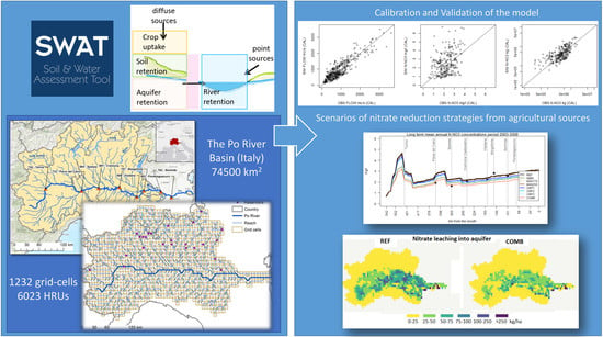
:Water contamination caused by the presence of excessive amounts of nitrate can be catastrophic for aquatic ecosystems and human health. Due to these high risks, a great deal of emphasis has been placed on finding effective measures to reduce nitrate concentrations in rivers and aquifers. In this study, we used the SWAT model based on grid-cells of 5 minutes of resolution for assessing the processes involved in nitrate loads generation and transport into aquifers and rivers and for providing basin management strategies of nitrate reduction. We applied the model in the Po River Basin (Italy), one of the most densely populated and highly agriculturally exploited area in the Mediterranean basin. The model was successfully calibrated and validated in eight monitoring stations along the Po River for the period 2000–2012. Simulated monthly streamflow and nitrate concentrations were in good agreement with observations, obtaining values of bias around ±25% in both calibration and validation. Among the tested scenarios of nitrogen reduction from agricultural sources, red clover cover crop after corn, coupled with a targeted reduction of mineral fertilizers and the limitation of nitrogen manure leads to a reduction of nitrate leaching and nitrogen emissions of around 37%.
1. Introduction
High nutrient concentrations in surface water and groundwater are still a major cause of water quality degradation. One of the main negative consequences of such degradation is eutrophication of water resources still pervasive in many lakes, coastal areas and rivers of the world due to diffuse nitrogen and phosphorus emissions that are the main drivers of this phenomenon [1].
In regions with intensive agriculture, surface water and groundwater are usually affected by anthropogenic pollution resulting from the use of high doses of fertilizers and inefficient irrigation techniques [2]. Indeed, fertilization input is recognized as the main diffuse source of nitrate contamination of water in agricultural areas [3].
The application of large amounts of mineral and organic fertilizers can contribute to excessive nutrient losses in rivers and groundwater. These losses can occur via surface runoff, sub-surface flow and leaching into aquifers. As a consequence, EU legislation, such as the Nitrates Directive [4] and the Water Framework Directive (WFD) [5], have enforced the limitation of nutrient losses to freshwater bodies through more careful management of agricultural land [6]. In particular, the Nitrates Directive requires the designation of nitrate vulnerable zones (NVZs)—areas which are polluted or at risk of being polluted by nitrates from agricultural nitrate pollution, where Codes of Good Agricultural Practice must be put in place to reduce or control nitrate losses. Quantifying the effectiveness of these practices is key to the successful implementation of the directive. Indeed, the directive requires competent authorities to report monitoring data to assess its state of implementation. However, short-term monitoring data cannot completely capture the efficiency of measures put in place because of the lag time characterizing nutrient processes [7]. In this context, mathematical models can overcome this limitation allowing to identify and evaluate effective management strategies.
Modelling is considered extremely valuable as it can help quantifying the pollution and identifying its sources, and guiding decisions to improve management [8,9]. In particular, models were used in the initial stages of the WFD implementation to perform analysis of pressures and impacts, as well as during the design, setting up and surveillance of the monitoring networks and for the development of River Basin Management Plans [7].
There is a wide range of models with a large diversity of complexity and capabilities for simulating the impact of nitrogen mitigation measures, ranging from empirical methodologies (e.g., EXPORT coefficient [10]), conceptual models (e.g., GREEN-Rgrid [11]), to physical-based models (e.g., Soil and Water Assessment Tool, SWAT [12]). Their capabilities depend on the purpose for which they were developed. Their complexity and data requirements increase with the number of processes that they represent [7].
Scenarios of nutrient reduction discharge in the Mediterranean Sea are available [11], however they focus mostly on nutrient reduction at the source, assuming no impact on crop production and without considering the lag time in terms of response to a change in management. Consequently, in order to evaluate realistically the efficacy of measures in river basins, more detailed process-based models able to simulate in integrated way the impacts of agricultural management on water quality must be used.
The Soil and Water Assessment Tool (SWAT) [12] is one of the most used models for long-term simulation in predominately agricultural watersheds because it integrates the soil water and nutrient processes consistently, together with their impacts on crop growth and catchment hydrology [9,13,14,15].
In the Mediterranean area, the Po River Basin (Italy) is particularly problematic, with its surface aquifers containing generally high levels of nitrates, particularly in the lower Piedmontese plain (near the source of the Po River), in the Milan valley (central area of the Basin) and in the Emilia–Romagna plain (southeast area of the Po River Basin) [16]. About 22% of the basin was identified as NVZ, 80% of water withdrawal for civil and industrial comes from aquifers [17], and nitrogen leaching is the main problem affecting the quality of groundwater [18].
In the basin, approximately 70% of nitrogen (N) loads come from diffuse sources while 30% from point sources [19], and annual total nitrogen and nitrate (N-NO3) loads transported to the Adriatic Sea in the period 2003–2007 were estimated at 166,552 ton/y and 86,295 ton/y, respectively [11]. Therefore, the reduction of nitrate concentration in aquifers and rivers of the Po Basin should focus on reducing diffuse nitrate losses from agriculture, by looking at alternative management options including mineral fertilizers strategies, manure management, and cover crops as conservation practice.
To test these hypotheses, we applied the SWAT model in the Po River Basin using a grid-cell approach employing the most recent global readily available datasets, with the following main objectives: i) calibrate and validate monthly streamflow, nitrate concentrations and loads in surface water in the Po River Basin, ii) provide long term mean annual water and nutrients balances for identifying the main pathways of nitrate pollution, iii) identify hot spots of nitrate contamination in rivers and aquifers that breach European drinking-water standards, iv) evaluate the effectiveness of diverse agricultural management strategies in reducing nitrate leaching and nitrogen emissions.
We start with briefly describing the Po River Basin, and then we give details about the model set-up, calibration and validation. Next, we present seven scenarios of nitrogen reduction from agricultural sources, and finally we discuss the results including the best alternative management practices to reduce nitrate leaching and identifying hot spots of nitrate concentration along the Po River where management efforts should focus.
2. Materials and Methods
2.1. Study Area: The Po River Basin
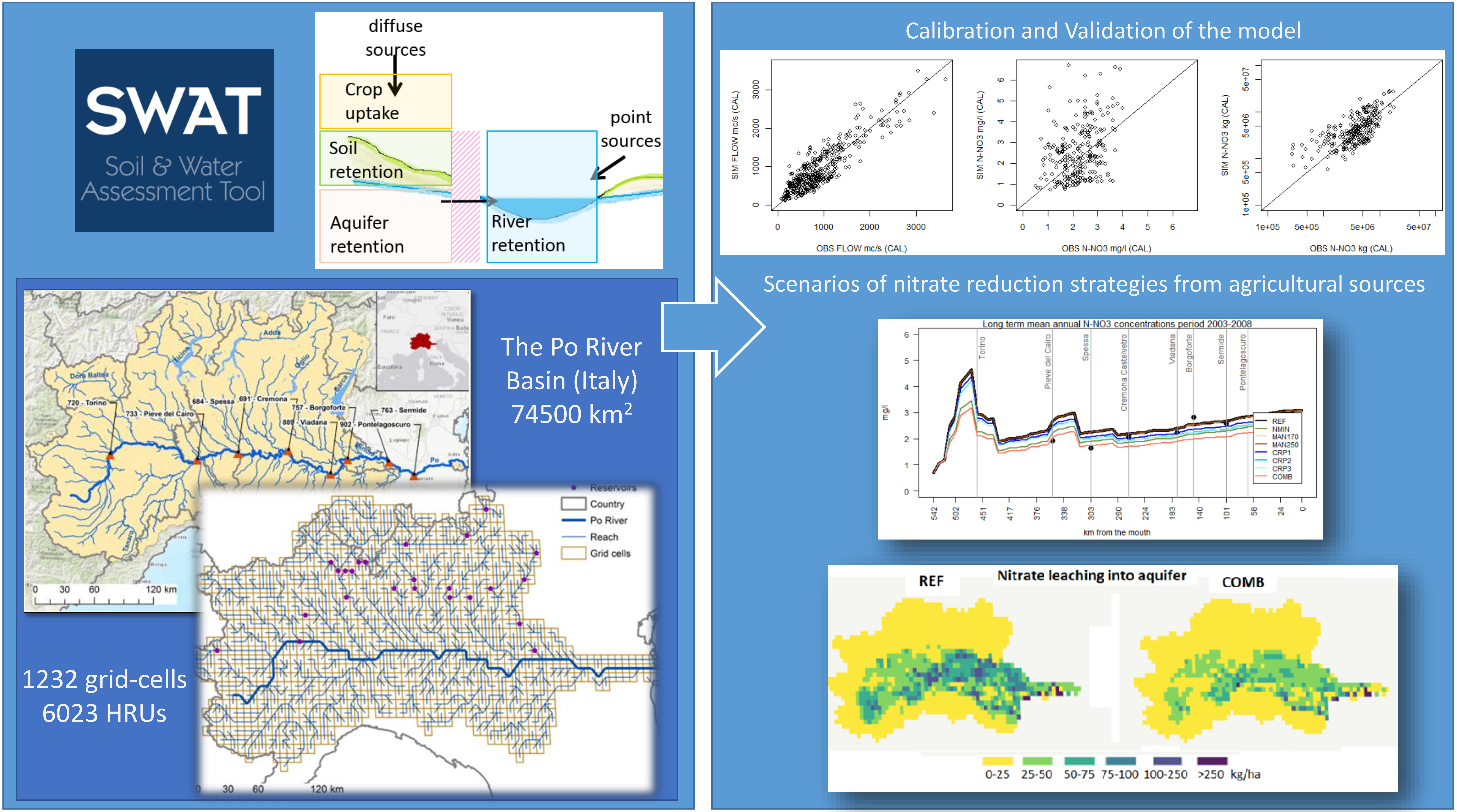
The Po River Basin is the largest Italian river system, with an area of about 74,500 km2, a stream length of 652 km, 141 tributaries, 450 lakes and a delta area of 380 km2 [20]. The basin covers seven Italian regions, and includes part of the Canton Ticino in Switzerland (Figure 1). Climate is influenced by the orography: it is typically alpine in the mountain zone, continental-warm in the flat basin area and Mediterranean on the coast. The average annual temperature is around 14 °C, ranging between 3 °C in winter and 25 °C in summer. The average annual precipitation is about 980 mm/y and the average discharge at Pontelagoscuro near Ferrara (Figure 1a) is around 1500 m3/s (period 1986–2001). The basin can be divided into three geographical regions: the Alps, the Apennines and the Po valley, where most of the economic and agricultural activities take place [19].
Approximately 33% of the studied area is agricultural (crops and fodder), 34% is forest and 25% is managed grassland (Table 1). The main crops are rainfed and irrigated corn, followed by rainfed wheat and irrigated rice. About 6% of the basin is irrigated (Table 1).
Water withdrawal for civil and industrial use is about 5 km3/y, 80% of which is withdrawn from aquifer, while annual water use for irrigation is about 17 km3, of which 91% is abstracted from surface water [17].
2.2. Model Description and Baseline Set-up
The Soil and Water Assessment Tool (SWAT; [12]) model is a process-based, semi-distributed model. It is widely used in large river basins to simulate water quantity and quality [21,22,23]. The model was selected because it has a flexible structure allowing to address different water resources and pollution problems, and it is well documented and open source. In this study, SWAT version 2012.664 was used to simulate water quantity and quality in the Po River Basin and to assess the effectiveness of several selected strategies for the mitigation of nitrate emissions to aquifers and rivers.
The model operates at daily time steps and its major components include hydrology, plant growth, nutrient cycles, and land management [14,24]. In SWAT, a watershed is divided into subbasins, which are further subdivided into hydrologic response units (HRUs) that consist of unique combinations of soil, land use, and slope. The model structure comprises two phases: a land phase solved at HRU level, and a stream phase solved at reach level [25]. In the land phase, the HRU water, sediment and nutrients cycles in soil, and losses are simulated and then aggregated at the subbasin level. The movement of water, sediments, and nutrients through the stream are simulated in the routing (stream) phase.
SWAT requires input data related to topography, land use, soil, climate and land management. In this study, the inputs were kept consistent with those elaborated for the GREEN-Rgrid described in Malagó et al. [11].
SWAT was forced to use a predefined delineation of streams and watershed using a regular grid-cell and a river network of 5 arc-minutes of resolution (about 60 km2 of grid cell area in the Po Basin). The imposed sub-basins and rivers in the Po consisted in 1232 regular polygons and segments. Consequently, hereafter we refer to grid-cells instead of sub-basins (Figure 1b). We chose to define sub-basins as regular grid-cells for several reasons. First, due to the rapid development of remote sensing systems, global spatial data (i.e., precipitation, soil characteristics, river network, population etc.) are available as raster format providing a more homogeneous information around the world. Consequently, different applications of SWAT can be easily compared, avoiding the uncertainty related to the use of different inputs. Second, the process of incorporating raster data into sub-basins instead of using directly grid-cells would require data transformation from a simple grid geometry to irregular polygons increasing the risk of loss of information and accuracy [26].
The digital elevation model (DEM) was retrieved from GTOPO30 [27] with a grid-cell of 30 arc seconds (approximately 1 km) that was rescaled at 100 m × 100 m of resolution.
The land use map was derived from 100 m × 100 m raster map built from the combination of the GLOBCOVER 2009 map [28] and Spatial Production Allocation Model (SPAM) [29] that provides crop-specific physical area, harvested area, and yields for 42 crops. Data are available for the year 2005 (average of 3 years centered on 2005) for four production systems: irrigated high inputs, rainfed high inputs, rainfed low inputs, and rainfed subsistence.
Soil type and characteristics were defined using the Harmonized World Soil Database [30]. For each grid-cell we considered the dominant soil and we used the top soil layer data for a maximum of 1-m depth. The available water capacity of each soil was calculated using the pedotransfer function proposed by Rawls et al. [31] and the saturated hydraulic conductivity was calculated using the Saxton et al. [32] equation.
Based on the combination of land use, soils and slopes, the Po Basin was discretized into 6023 HRUs with areas ranging between 180 and 6000 ha.
The global HydroLakes database [33] was used for identifying lakes and reservoirs on the river network. At most one single lake was included in each grid-cell, using the area and volume parameters from the HydroLakes. In the Po River Basin, 25 major lakes were included for a total area of around 90,000 ha.
Daily precipitation was obtained from the global gridded MSWEP dataset at 0.25 degrees resolution [34]. Daily data for the other atmospheric forcing variables (temperature, solar radiation, wind speed and relative humidity) were obtained from ERA-Interim [35]. The whole dataset of climate data covers the period 1979–2012. To account for the increase in precipitation with elevation, that is typically observed in mountainous regions, four elevation bands were implemented [25].
The nutrient emissions from point sources were estimated based on urban and rural population, emission rates per person, the percentages of urban and rural population connected to wastewater treatment plants and their treatment technology level as explained in detail in Malagó et al. [11]. The water discharge from point sources was calculated using the amount of withdrawals for domestic uses provided by [36]. These values were also used as abstractions from deep aquifers in SWAT.
The daily nitrogen atmospheric deposition in each grid-cell was derived from a global map of 1 degree resolution of the World Data Centre for Precipitation Chemistry (http://wdcpc.org/).
The modelled crop management consists of planting, fertilization, irrigation, tillage and harvesting operations. The timing of management operations was implemented according to the heat units accumulated by crops [12]. The crop calendar was retrieved from the global dataset MIRCA2000 [37]. This dataset provides the start and end of the cropping period for 26 irrigated and rainfed crops on 402 global spatial units.
The accumulated heat units (HU) for each crop were calculated using the average daily temperature dataset in the period 1979–2012 [35], the duration of the growing season and the base temperature parameter provided by SWAT. Crop growth only occurs on those days where the mean daily temperature exceeds the base temperature. The heat units accumulated in the cropping period are the sum of the differences between average daily temperature and the base temperature.
The amount of manure, mineral fertilization, and irrigation were retrieved from Malagó et al. [11] for the year 2005 and kept constant through the simulation. One single application of N and P manure and N, P mineral fertilizers was used for each crop, managed grassland and fodder crop. For irrigated crops 10 applications of water were scheduled during the growing period. Two types of tillage (disk chisel and harrow 10 bar) were used before the application of manure. Table 2 reports an example of management for irrigated corn.
The annual irrigation (mm) for each irrigated crop was calculated applying a downscaling procedure based on the irrigation volume (m3) reported at country level for 26 crops by Siebert and Döll [38], the irrigated area in each cell retrieved from SPAM, and the difference between the potential evapotranspiration and precipitation as described in Malagó et al. [11].
The initial values of nitrate concentrations in the shallow aquifer required to initialize the model were derived putting in relation reported observed nitrate concentrations with environmental variables including climatic, soil, hydrological, and management data using a stepwise regression approach [39].
The simulation period covers 13 years from 2000 to 2012, in addition to 21 years of warm-up used to initialize model variables and allow processes to reach a dynamic equilibrium [40].
2.3. Calibration, Validation and Evaluation
The calibration of SWAT was performed following a cascade modelling approach starting from crop yield, then streamflow and finally nitrate concentration. The monitoring stations are located along the whole Po River as described in Table 3. These stations were selected since they provide important insights on model performance in estimating overall nutrient loads [19].
To assess the model performance for both calibration and validation, we used the percent bias (PBIAS) as recommended by Moriasi et al. [41].
PBIAS measures the tendency of the simulated data to be higher or lower than the observations. Values close to 0 indicate a lack of bias (neither underestimation nor overestimation). Positive and negative values indicate an overestimation and underestimation of the simulated data, respectively. We considered PBIAS values in the range of ±25% for monthly streamflow, nutrient concentrations and loads to be good and acceptable.
The modified coefficient of determination bR2 was used in the calibration process for identifying the best parameter set for streamflow and nitrate concentrations. The percent bias and bR2 were calculated using the R package “hydroGOF” [42].
2.3.1. Crop Yields
Crop yield calibration was based on the comparison of long-term average annual crop yields for the simulation period 2000–2012 with the annual values centered on 2005 provided by SPAM, and with the national statistics reported by FAOSTAT [43]. Since SWAT estimates dry crop yields, we converted SPAM and FAOSTAT yields from fresh to dry weights using crop moisture contents retrieved from Williams at al. [44] as described in Malagó et al. [11].
The crop calibrated parameters are reported in Table 4. In particular, the base temperature for bare, shrub, and grassland was set to 1 °C and to 3 °C for fodder crops. The radiation use efficiency was decreased from the default values to 5 and 20 kg/ha/MJ/m2 for fodder crops and irrigated sugar beet, respectively. The parameters for rice were adjusted using the values proposed by Yang et al. [45].
2.3.2. Streamflow
The calibration of monthly streamflow was performed applying a regionalization technique of calibrated parameters in large river basins in Europe in previous SWAT studies, followed by an adjustment of the most sensitive parameters using the SUFI-2 method [46]. Times series of monthly streamflow for 8 monitoring stations along the Po River were divided into calibration and validation periods: 2005–2012 and 2000–2004, respectively.
In order to provide a more reliable evaluation of nitrate leaching into aquifer, only groundwater parameters were estimated by regionalizing values calibrated in previous large-scale applications in Europe: Spain and Scandinavian Peninsula [21], the Danube River Basin [22] and France [47]. The regionalization consists of a cluster analysis performed using the Self Organized Map (SOM) [48] and a similarity approach to transpose the calibrated parameters to all uncalibrated grid-cells [49]. These parameters, available for 61,439 cells in Europe, include: the groundwater delay (GW_DELAY, days), the baseflow alpha factor (ALPHA_BF, days), the threshold depth of water in the shallow aquifer required for return flow to occur (GWQMN, mm), the groundwater transfer from the aquifer to the unsaturated zone coefficient (GW_REVAP), the threshold depth of water in the shallow aquifer for capillarity rise (REVAMN, mm) and the fraction of groundwater recharge to deep aquifer (RCHRG_DP).
The SOM is a modified artificial neural network characterized by unsupervised training that can project high-dimensional information into a low-dimensional array [50]. In the SOM, input samples are compared based on the variable characteristics and mapped onto vectors referred to as neurons and are positioned closed to each other on a matrix referred as a map. The neurons are thus grouped into clusters, where neurons are similar to each other. The cluster analysis was performed using the Ward’s agglomerative hierarchical clustering method [51] that is based on a least-squares criterion, producing clusters that minimize within-cluster dispersion. In this study, training samples consist of 61,439 grid-cells characterized by the following features affecting the groundwater processes: elevation (m), slope (%), sand and clay content (%), organic matter content (%), the percentage of different classes of land cover, average annual precipitation (mm), average annual temperature (°C), average streamflow (m3/y), irrigated area (ha) and aquifer permeability (m/day).
The SOM method was applied to the training dataset and 13 clusters were obtained. The optimal number of clusters was selected using 30 indices based on the R NbClust package [52]. To assign all the remaining grid-cells to each cluster, the grid-cells of the test were associated to the SOM defined neurons using a predictive function based on the minimization of the Euclidean distance and consequently the cluster were identified based on the association of neuron-cluster.
Finally, inside each cluster the training grid-cells were used as donor to transpose the groundwater parameters in the uncalibrated grid-cells using a classification procedure based on hydrologic similarity [49].
After the regionalization, the transposed groundwater parameters were calibrated using the SUFI-2 algorithm in two steps that consist on: 1) changing all groundwater parameters in the range of +-50%, and the best parameter set was obtained among 100 combinations maximizing bR2 between simulated and observed monthly streamflow; 2) reducing the set of groundwater parameters to the most sensitive ones, decreasing also the range for relative changes as reported in Table 4, and the final set of groundwater calibrated parameters were obtained from 100 simulations by maximizing bR2 (Table 4).
2.3.3. Nitrate Concentrations
The nitrate concentrations were calibrated in 6 monitoring stations in the period 2005–2012 by changing the mineralization rate of active organic nitrogen and the nitrate half-life in the shallow aquifer. The best parameter set was obtained among 100 simulations by maximizing the bR2 between simulated and observed monthly nitrogen-nitrates concentrations. The model was then validated in the same stations for the period 2000–2004. Finally, the model was evaluated comparing simulated and observed monthly loads for the whole period of simulation 2000–2012.
2.4. Scenario Analysis
Different basin management scenarios were developed for assessing the efficiency of mitigation strategies for nitrate reduction in the Po watershed. The strategies focused both on nutrient reduction at the source (mineral and manure fertilizers) and on crop management with the introduction of a winter catch crop during the fallow period following corn harvest.
The nitrogen mitigation strategies were formulated in seven management scenarios of agricultural practices (Table 5) that were implemented in cropland area (16% of the whole watershed). The selected crop area consists of 2208 HRUs with areas ranging from 180 to 5200 ha.
The first scenario (NMIN) consists of a reduction of mineral fertilizer application in agricultural HRUs ensuring that the annual crop yield would not decrease more than 5% from the baseline in order to guarantee the farmers income. Scenarios MAN170 and MAN250 were developed to mimic the restrictions imposed by the Nitrates Directive [4]. In NVZs, the Directive limits the use of manure to 170 kg/ha, or 250 kg/ha in case of derogation. Other scenarios tested the use of cover crops after the harvesting of corn, the main spring-summer crop in the basin. Cover crops were implemented in 730 HRUs.
Cover crops protect against erosion between two corn growing seasons; they build up the organic matter in the soil following their killing [53], and they assimilate nitrate, reducing leaching during the winter. Three scenarios of cover crops were implemented. The first (CRP1) uses rye as cover crop. The second (CRP2) uses rye as cover crop after harvesting the corn, for which the mineral fertilizer application is reduced, and an example of management is reported in Table 2. The third (CRP3) is the same of CRP2, but red clover is used instead of rye. Red clover provides many benefits such as fixing nitrogen to meet the needs of the following crop, protecting soil from erosion, competing with weeds, as well as supplying forage [54]. Finally, a mixed scenario was tested combining the strategies implemented in other scenarios: (i) reduction of mineral nitrogen fertilizer in all crop fields (2208 HRUs) (NMIN); (ii) manure application below 170 kg N/ha (MAN170); (iii) use of red clover as cover crop after harvesting corn (CRP3).
Each of the seven scenarios of Table 5 was simulated for the period 2000–2012 and compared with the baseline simulation results (REF).
3. Results
3.1. Analysis of Model Calibration and Validation
3.1.1. Crop Yields
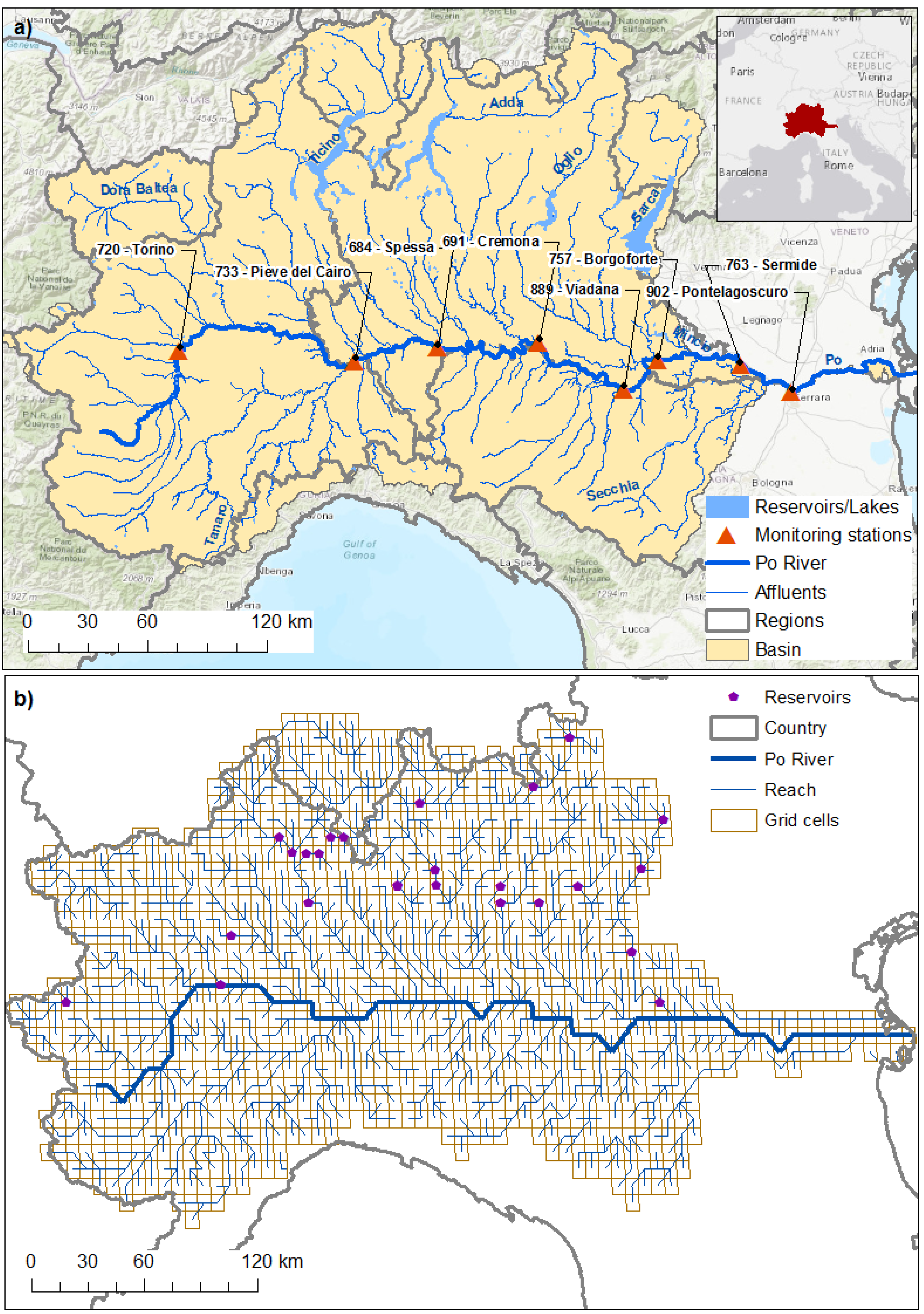
Crop yields were calibrated considering the whole period of simulation 2000–2012. The results were satisfactory as the predicted annual crop yields compared well with both SPAM and FAOSTAT values (Figure 2). Relatively large overestimations were observed for sorghum, potatoes under highly intensive management and vegetables (HSOR, HPOT and e.g., HVEG, see Table A1 in Appendix A for the description).
The annual variability of yields of dominant crops, low intensive corn (LMAI) and irrigated corn (IMAI), were well captured as shown by the strong correlation between SWAT and FAOSTAT values (Table 6). The predicted yields for wheat exhibited low correlation with the values reported by FAO, and the standard deviation of wheat annual yields was 1.2 ton/y and 0.35 ton/y respectively for SWAT and FAOSTAT. This can be explained considering that FAO yields sum irrigated and rainfed productions. Irrigated rice yields resulted negatively correlated with annual FAO yields. The simulated SWAT values are strongly correlated with water stress (in years where water stress increases, irrigated rice yields decreased), while FAO yields follow an opposite trend.
3.1.2. Streamflow and Nitrates
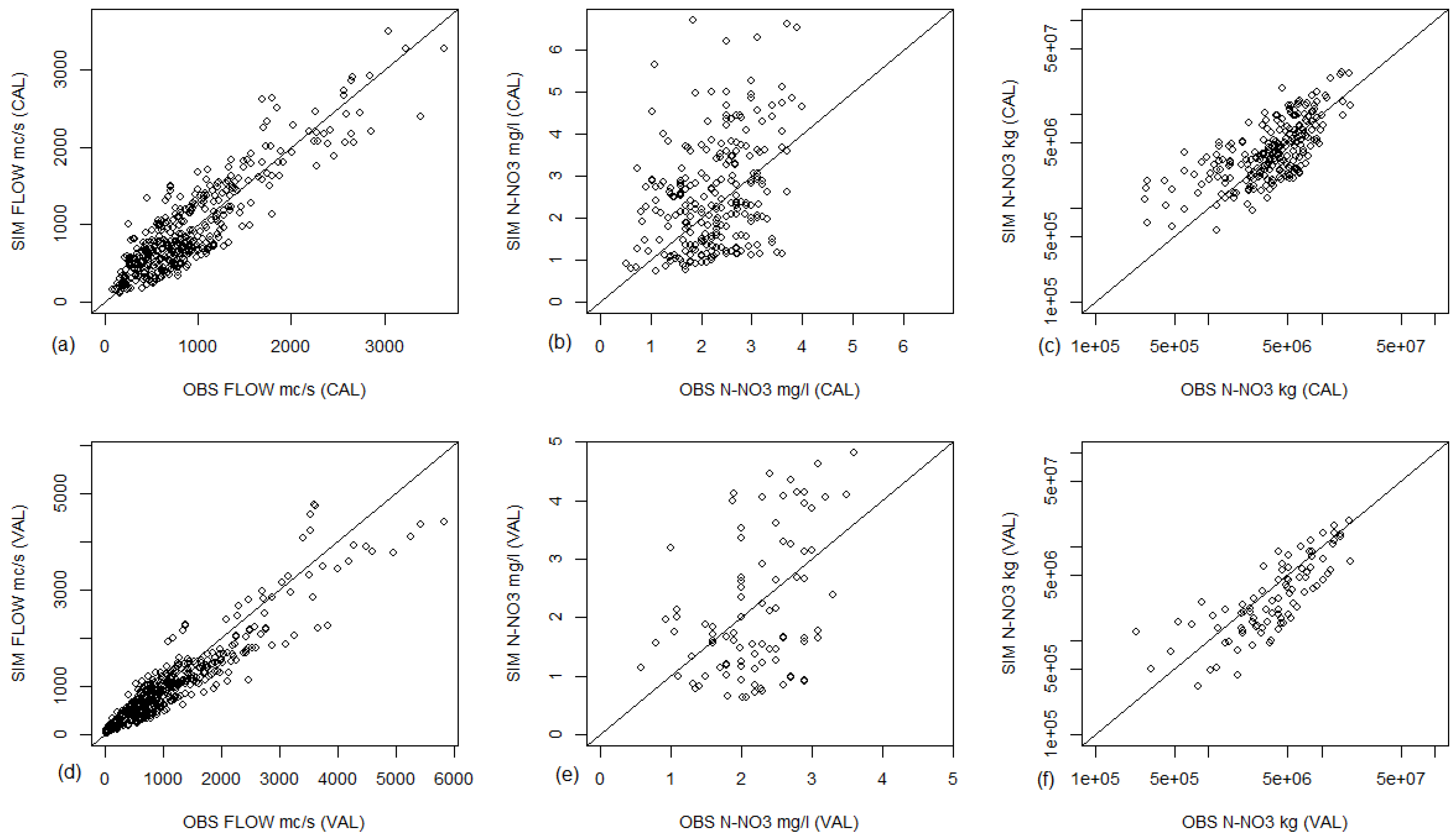
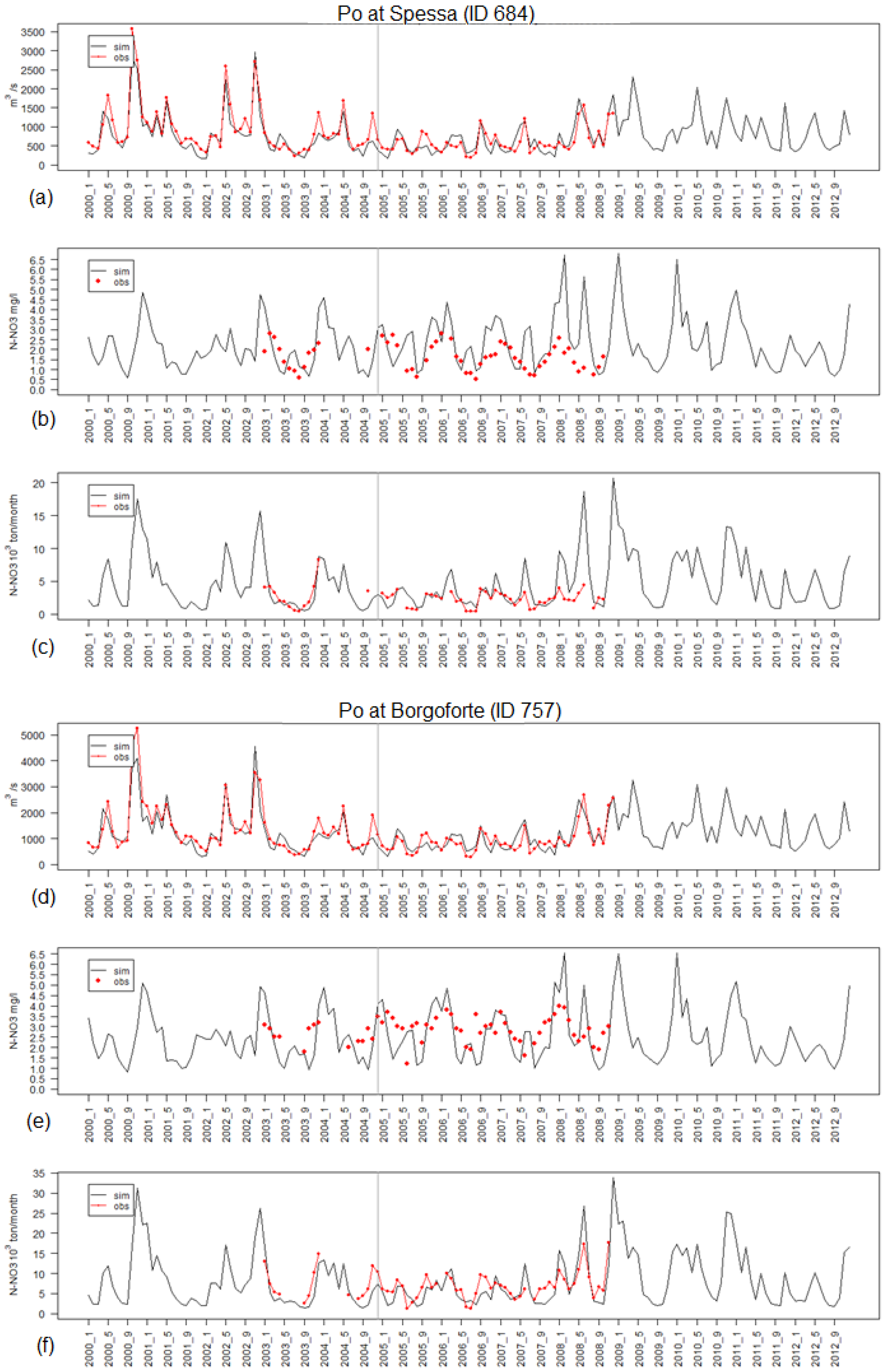
The performances of SWAT in simulating monthly streamflow are satisfactory both for calibration and validation (Table 7 and Figure 3). The PBIAS (%) was good for streamflow and N-NO3 concentrations according to the ratings proposed in Moriasi et al. [41]. The PBIAS% calculated between the observed and simulated monthly nitrate loads resulted also very good (Figure 3 and Table 7). Visual appraisal of monthly streamflow, concentrations and loads in Figure 4 confirmed that monthly variations were well captured and that peaks are well reproduced.
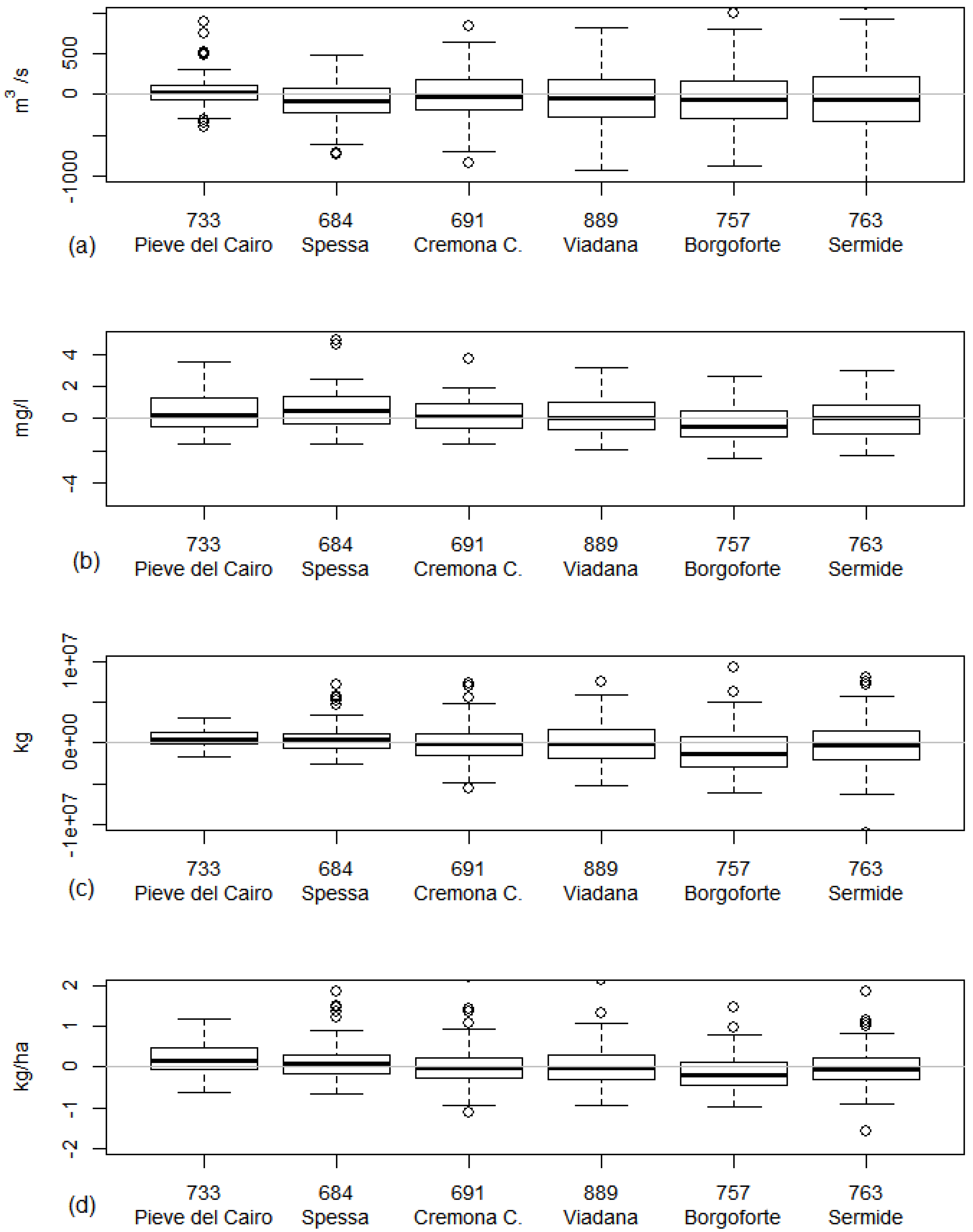
The residuals (simulated minus observed values) in six stations along the Po River were well centered on zero (Figure 5). However, some underestimations of simulated nitrate concentration can be observed in the lower stations near the mouth, and in particular for station Borgoforte at 147 km from the mouth.
3.1.3. Annual Water and Nitrogen Balance
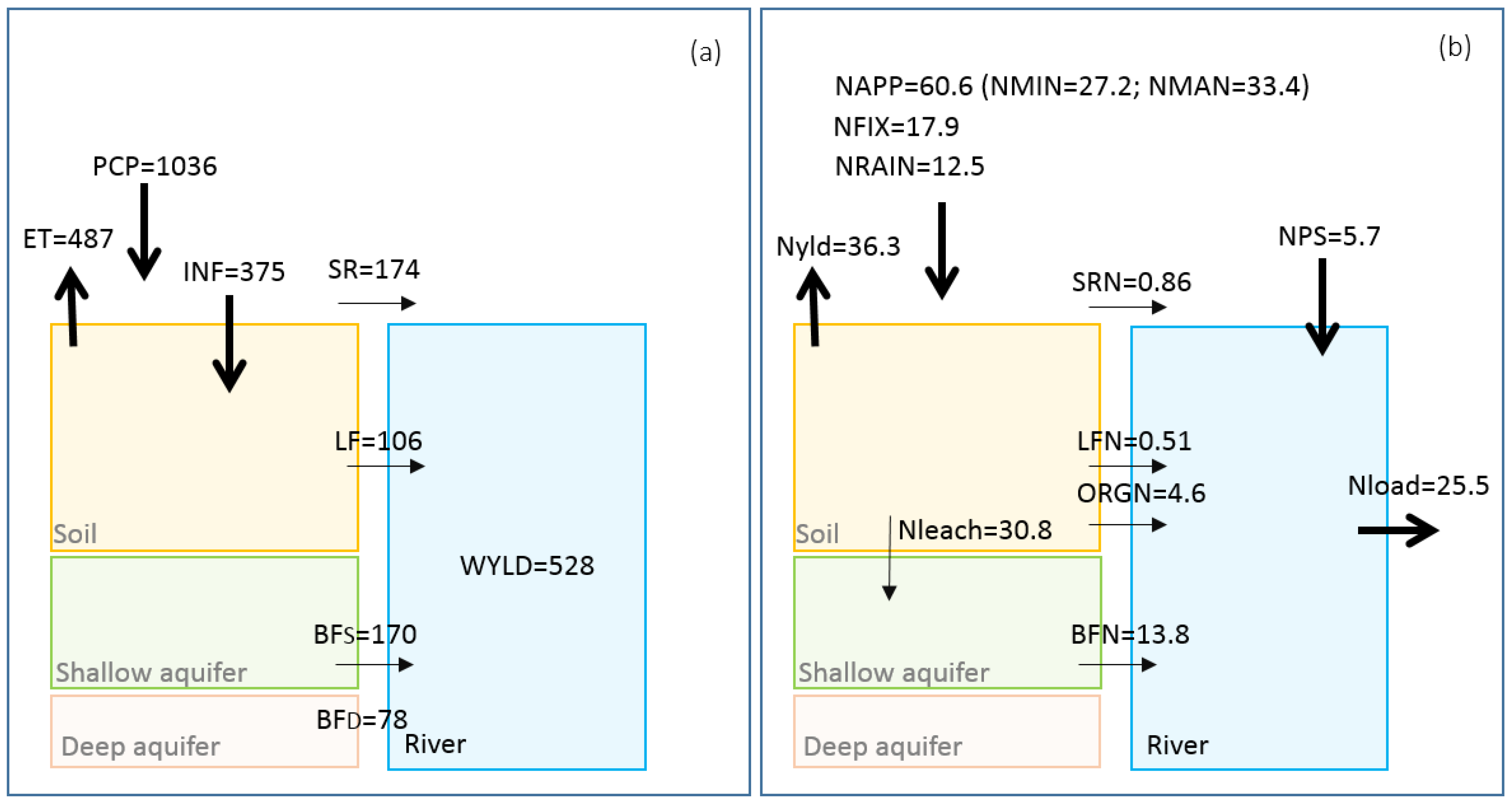
Figure 6 shows the long-term mean annual water and nitrogen balance for the entire Po River Basin (74,600 km2) as simulated by SWAT for the period 2000–2012. It was estimated that 47% (487 mm) of precipitation (PCP, 1036 mm) was lost through evapotranspiration (ET) and 2% as percolation in the deep aquifer, and 51% was discharged in the stream (water yield, WYLD, 528 mm). Surface runoff (SR) and baseflow from shallow aquifer (BFS) were the main pathways of water losses.
Regarding the nitrogen balance, the diffuse inputs were estimated at about 91 kg/ha consisting of 27.2 kg/ha mineral fertilizer, 33.4 kg/ha of manure, 17.9 kg/ha of nitrogen fixation and 12.5 kg/ha of atmospheric deposition. Point sources amounted to about 5.7 kg/ha. The nitrogen removed by crops and the nitrogen lost in the soil were estimated to be about 40% and 20% of nitrogen inputs, respectively. About 7% (5.9 kg/ha) of total inputs were emitted to the river while 33% (30.8 kg/ha) of total inputs leached to the aquifer. The largest contributor of the emissions to the rivers was the baseflow with about 13.8 kg/ha. The total nitrogen emissions to the river were estimated at 19.8 kg/ha, which together with point sources contributed to a load of about 25.5 kg/ha.
Diffuse and point sources were responsible of 78% and 22% of the total nitrogen load in the Po River. These estimations were comparable to those reported by other studies in the Po Basin [19,20]. In these studies, the diffuse sources were estimated to be around 70% and 60%, respectively, while the contribution of point sources amounted to about 30% and 40%, respectively. In particular, Palmeri et al. [19] estimated a groundwater contribution of 13.7 kg N/ha and surface runoff load of 0.65 kg N/ha.
The long-term annual average of nitrate loads at Pontelagoscuro were 115,000 ton-N/y, 93,460 ton-N/y, and 78,032 ton-N/y for the periods 2000–2012, 2003–2008 and 2003–2007, respectively. These values are consistent with those provided by other authors [11,19,20,55] (Table 8), as well as with the observations monitored at Sermide, the nearest station to Pontelagoscuro.
3.2. Analysis of Scenarios of Agricultural Practices
Table 9 shows the potential effects of different management strategies on nitrate fate in cropland areas for the period 2000–2012.
An analysis of the scenarios suggests that a targeted mineral fertilizer reduction of 23% from the baseline (NMIN) could decrease nitrate leaching and nitrogen emissions by 24% and 21%, respectively, with limited impact on crop yield. In particular, the main effect was observed in the reduction of nitrates transported via groundwater (BFN: 24% of reduction with respect to baseline) followed by nitrogen transported via lateral flow (LFN: 14%) and surface runoff (SRN: 13%). The highest reduction of organic nitrogen transported via sediment to river (ORGN) was observed in the scenarios of cover crops (from 33% of reduction of scenario CRP1 to 40% of scenario CRP3) explained by the decrease of sediment yield (SYLD) by about 50%.
The introduction of winter cover crops has a significant impact on nitrate reduction, and a limited impact on the water balance as reported in other studies [56,57,58]. Concerning the hydrology, we observed slightly lower water yields and higher evapotranspiration compared to the baseline. Rye and red clover cover crops reduced water yields in the cropland area from 301 mm (baseline) to 287 and 289 respectively, while evapotranspiration increased from 600 mm of baseline to 614 and 612 respectively.
The effect of winter cover crops in reducing nitrate leaching and nitrogen emissions is noticeable, in particular when coupled with a targeted reduction of mineral fertilizers. CPR2 scenario decreased nitrate leaching (Nleach) and nitrogen emissions (Nem) by 8% and 6% with respect to CPR1.
Red clover had additional benefits with respect to rye by reducing sediment yields by more than 50%, increasing the amount of nitrogen in the soil and consequently leading to an increase of crop yields in the Po River by about 18%. This was also pointed out by several studies as described in Marcillo at al. [59].
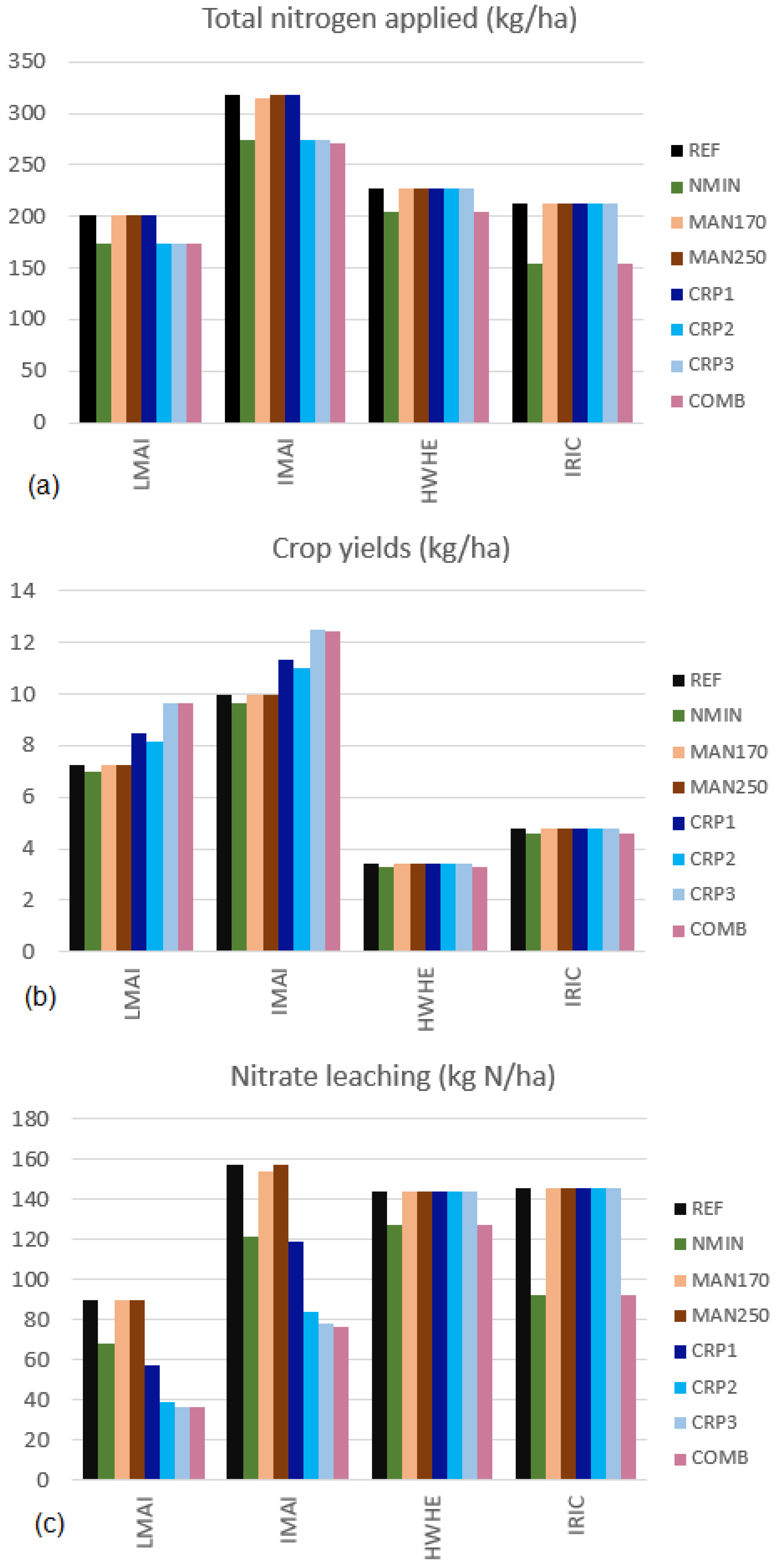
Figure 7 shows the changes of crop yields and nitrogen leaching for the main four crops in the basin in the tested scenarios. The effect of cover crops in scenario CRP3 on rainfed (LMAI) and irrigated corn (IMAI) is showing an increase of crop yields from the baseline by about 25% and 20%, respectively and a decrease of nitrate leaching by about 60% and 50%, respectively.
It should be noted that, albeit winter cover crops scenarios were implemented only on 5500 km2 (about 46% of crop land area in the basin), we obtained larger reductions of nitrogen leaching and emissions than those obtained in the more extensive NMIN scenario.
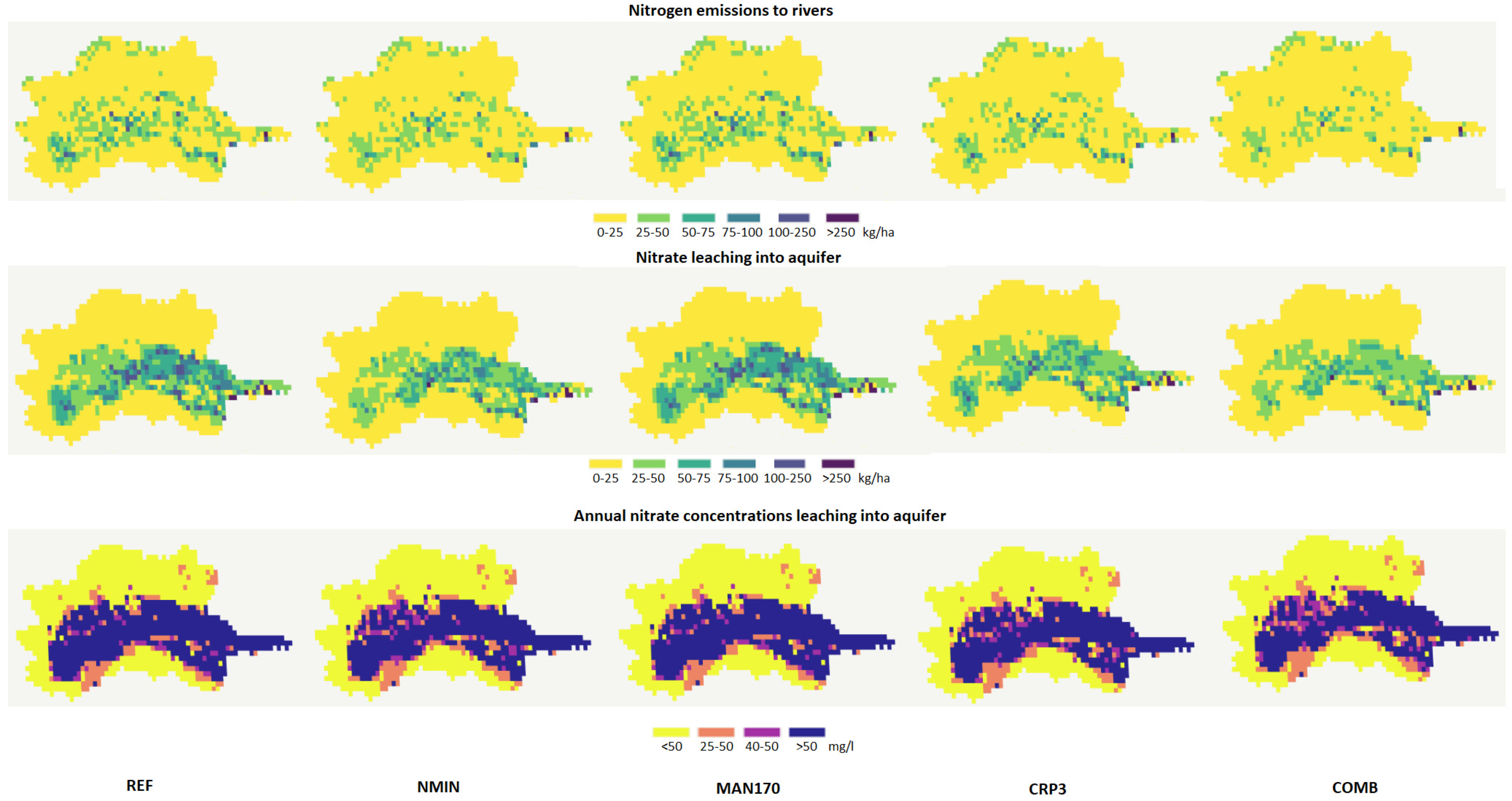
As expected, manure reduction scenarios are less beneficial in terms of N reduction in the river, but they bring significant local impacts (Figure 8), because the HRUs with N applications greater than 170 and 250 kg/ha were respectively only 71 and 9 covering respectively 332 km2 and 40 km2.
The mixed effect of red clover implementation after harvesting corn, with the targeted reduction of mineral fertilizers and the limitation of nitrogen manure to 170 kg/ha (COMB) had the highest impact on nitrogen reduction, maximizing the reduction of sediment yields and maximizing crop yields (Table 9, Figure 7 and Figure 8).
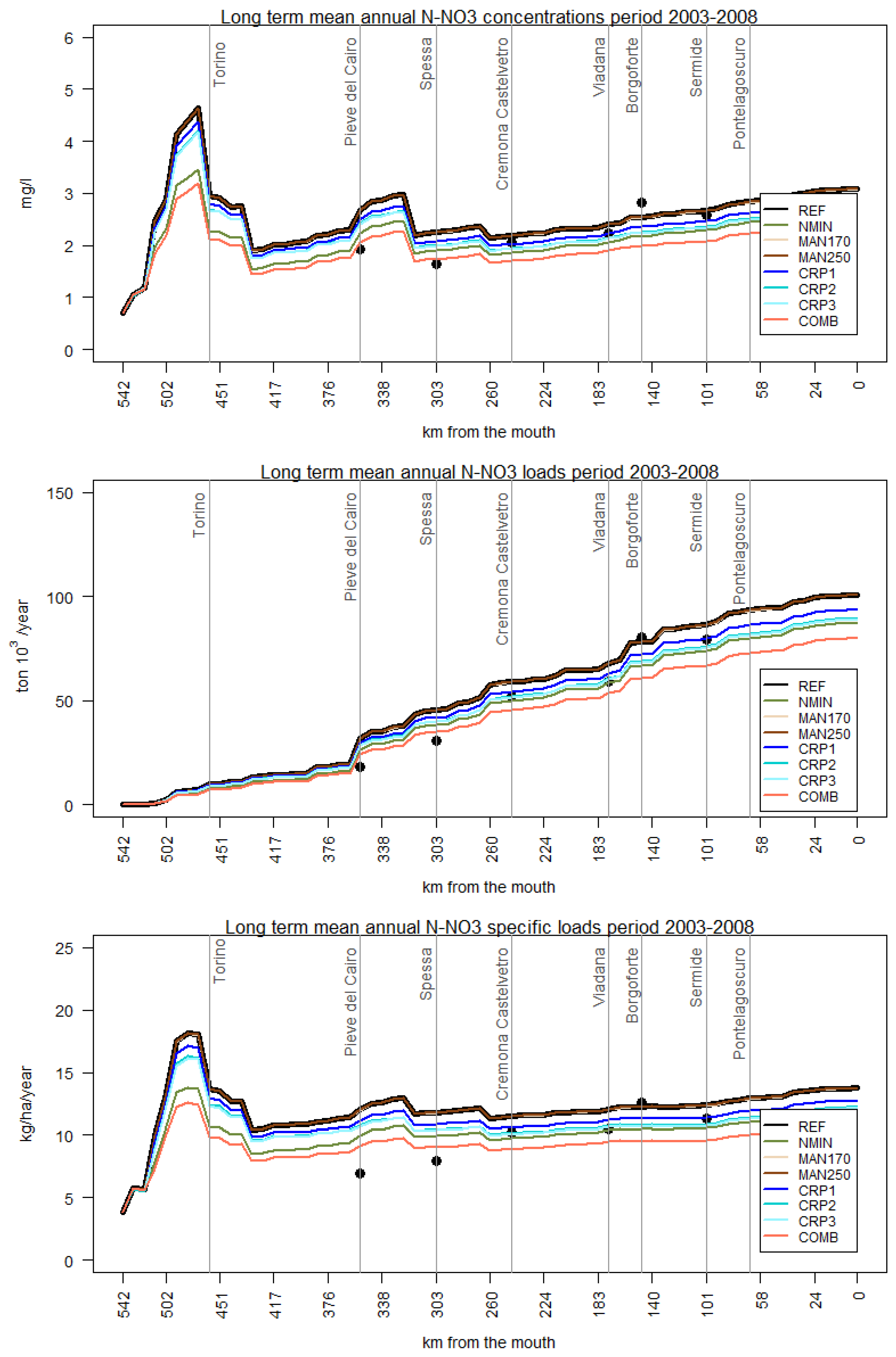
We have also observed that COMB and NMIN scenarios have the largest impacts in the reduction of concentrations and loads in the Po River (Figure 9), improving water quality all along the river from source to mouth.
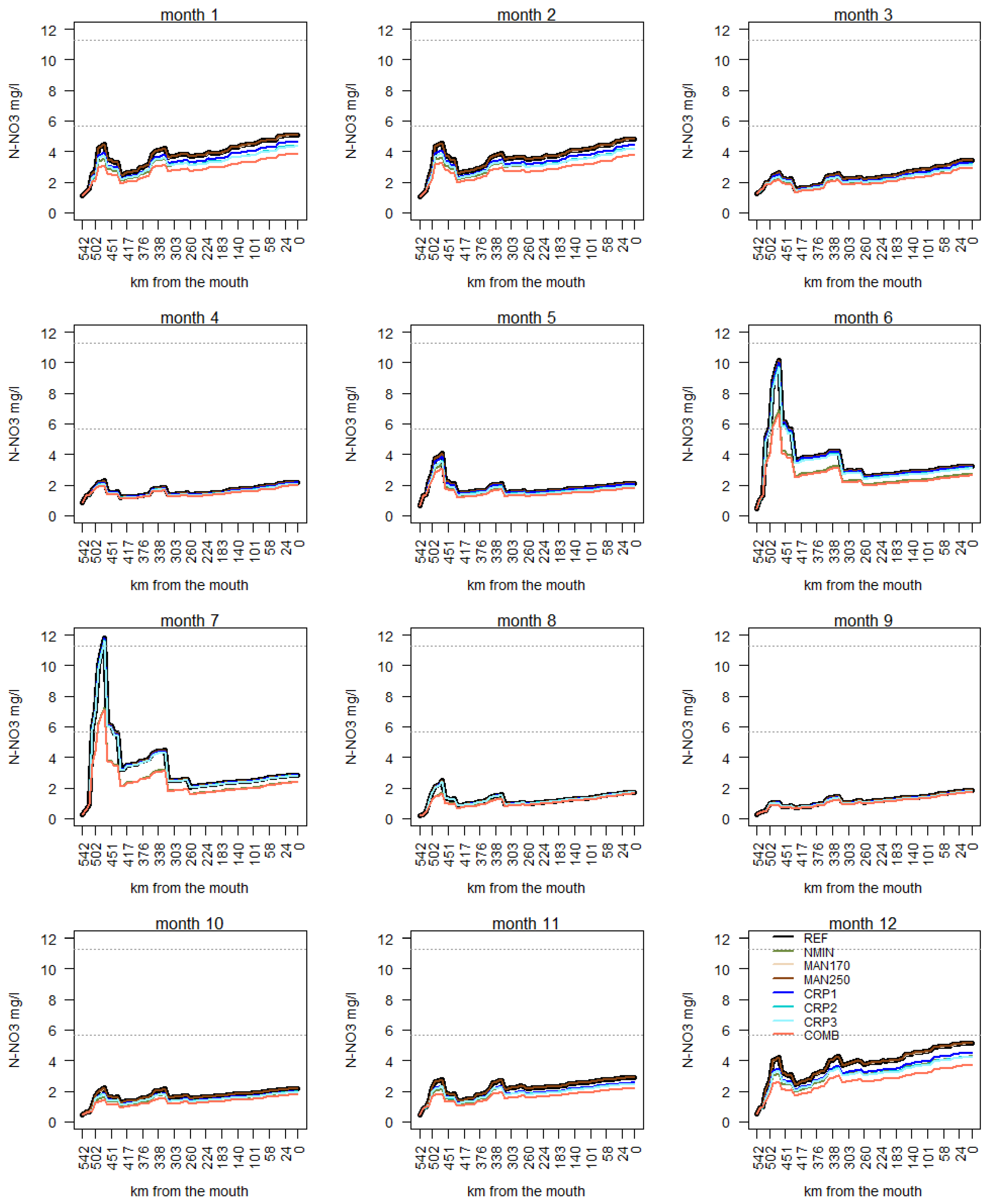
The evolution of the nitrate concentration along the Po River is shown in Figure 9. It is noteworthy that along the Po River three concentrations peaks were simulated before the junction of Dora Riparia with Po at Turin (km 473 from the mouth), before the confluence of the Ticino River (330 km from the mouth) and Adda River (278 km from the mouth). These peaks reached the highest values during June–July in the baseline simulation, exceeding 25 mg/L near Turin (Figure A1).
Our results capture the degree of groundwater nitrate contamination in shallow and deep aquifers in the western Po plain between Turin and Cuneo cities. In those areas, 37.6% of agricultural areas are NVZs, with 50% of the monitored points with nitrate concentration between 25 and 50 mg/L, and 24% larger than 50 mg/L [18]. Consequently, as the groundwater flows into the Po River before Turin [60], large amounts of nitrate are concentrated there (Figure 9, Figure A1 and Figure A2).
The main sources of nitrate contamination in this area are mineral fertilizers and manure [18]. The COMB scenario predicts a substantial reduction of nitrates concentration in this part of the Po River, suggesting that a combination management option may be an efficient strategy to reduce nitrate contamination.
In other sections of the Po River the simulated concentrations remain quite constant (Figure A1 and Figure A2), albeit several tributaries, such as the Oglio River, drain areas with large nitrogen surplus from agriculture. In particular, Bartoli et al. [61] found that the nitrate concentrations in the Oglio River, in its tributaries, in groundwater and springs, are greatly reduced by the denitrification in wetlands that are hydraulically connected with the river network.
4. Discussion and Conclusions
The global increase in the use of nitrogen synthetic fertilizers and manure over the last several decades has led to a degradation of water quality, especially in agricultural areas.
In Europe, several EU policy measures exist for controlling nitrogen emissions in the environment. In particular, the main objective of the Nitrates Directive is to “reduce water pollution caused or induced by nitrates from agricultural sources and prevent further such pollution”. This directive forces member states to set up monitoring systems, to designate vulnerable zones, and to activate protection plans that must contain mandatory measures related to the definition of a code of good agricultural practices, including balanced N fertilization, and to limit the amounts of animal manure (170 kg/ha/y) applied to land.
Italy transposed the directive in national legislation in 1999 (D.Lgs. 152/99). The national legislation transferred responsibility for identifying vulnerable zones to the regional authorities (Regions). The Po River Basin was, and still is, particularly problematical, with its shallow aquifers containing generally high levels of nitrates in the Cuneo–Turin plain, Alessandria area, in the north of Milan and in the Emilia–Romagna plain [16]. This is confirmed by our findings that highlight how current land management, after 20 years from the implementation of the Nitrates Directive, still results in significant vulnerability of the Po valley to nitrate leaching from diffuse sources and requires further mitigation measures (Figure 8, Figure A2).
The scenarios tested with SWAT show that the implementation of good agricultural practices could lead to a significant decrease of nitrate losses both to aquifers and rivers. We show that a reduction by as much as 37% of nitrate losses (COMB scenario) could be obtained with limited effects on crop production. It must be noted that this reduction will not affect the eutrophication of the Northern Adriatic Sea since it is mostly phosphorus limited [62]. However, it will strongly affect the quality of both stream and groundwater, improving also the good ecological status of surface water bodies.
Simulated nitrate leaching in the aquifers and emissions to surface waters were effectively reduced applying a targeted reduction of fertilizers (NMIN) and using winter cover crops (CPR1, CRP2, CRP3). These results agree with De Maio et al. [16], who suggested reducing agricultural nutrient pollution in Europe by moving towards agricultural systems where the input (manure and mineral fertilizers) is commensurate with the requirements of the crops (output). However, the sole reduction of nitrogen fertilizers does not cope with the problem of soil erosion losses due to tillage and occurring in the period where no crop is growing. Instead, cover crops proved to be an effective strategy for controlling sediment yield and for reducing nitrate leaching and emissions by 53%, 22% and 24% respectively (scenario CRP3, Table 9). Cover crops are shown to be the most effective practice in the Po River Basin land types that can be characterized as deep and permeable soils in the classification by Rittenburg et al. [63]. In this environment, cover crops increase the residence time of nitrates in the soil layers, increase plant nitrogen uptake, reduce soil erosion and nutrients transported via sediments, and increases soil carbon content [64].
The scenarios related to the limitation of manure application as required by the Nitrates Directive were not effective for the whole watershed as the spatial extent of implementation is extremely limited. With scenario MAN170 we can reduce the manure application on cropland by 2% (1200 ton of N manure; 36 kg/ha), while with scenario MAN250 by 0.2% (118 ton of N manure; 3.5 kg/ha) (Table 9). Similar conclusions were reported by De Wit et al. [65], who highlighted that the Nitrates Directive implementation resulted in significant local improvements of environmental conditions, but not in substantial reductions of N and P loads in large European river basins. It must be noted that our scenarios simulated the reduction of manure application assuming that the unused manure was lost. A better management of large quantities of manure available in limited areas, such as manure distribution networks, would allow the reduction of mineral input requirements, thus ensuring economic sustainable yields, and to limit pollution from diffuse sources. Solutions to manage the excess of manure could include i) the transfer outside the farm; ii) transformation or treatment (e.g., methanisation, composting or biological treatment); iii) burning for cement works [66]. These options can provide additional income for the farmers.
In this assessment, we showed that a reduction of nitrate losses could be achieved without affecting the economic sustainability of farmers. We further show that a combination of both nitrogen application reduction and the introduction of catch crops in rotation with typical crops of the Po River Basin could reduce nitrate losses into aquifers by as much as 20% (CRP3 scenario). The use of catch crops is particularly efficient considering that the nitrate losses in the Po watershed come mostly from the shallow aquifers. Thus, reducing nitrate leaching is particularly recommended in the flat part of the watershed. Winter crop cover strategy is more efficient in the hilly part of the watershed.
The use of the SWAT model is extremely efficient in identifying the types of measures depending on the local conditions.
Future work will focus in assessing how the proposed measures will perform under a changing climate. Indeed, expected climate change in the Mediterranean will include a decrease of precipitation during spring and summer and increase in fall and winter, while temperatures will increase throughout the year [67]. Crop management will be affected: an increase of irrigation is expected, while the increase of precipitation during fall and winter might yield large nitrate leaching. The increasing temperature will also affect the nitrogen cycle, leading to an increase of mineralization. Additional measures might have to be put in place to offset these expected changes.
Author Contributions
Conceptualization, A.M. and F.B.; Data curation, A.M. and F.B.; Formal analysis, A.M. and F.B.; Investigation, A.M., F.B., M.P. and E.G.; Methodology, A.M. and F.B.; Project administration, F.B.; Resources, A.M., F.B., M.P. and E.G.; Software, A.M. and F.B.; Supervision, A.M. and F.B.; Validation, M.P. and E.G.; Visualization, A.M.; Writing–original draft, A.M.; Writing–review & editing, F.B., M.P. and E.G.
Conflicts of Interest
The authors declare no conflicts of interest.
Appendix A

Table A1.
SWAT crop code and description.
| Crop Code | Crop Name | Management Type |
|---|---|---|
| HBAR | Barley | Highly intensive |
| HMAI | Corn | Highly intensive |
| HOOI | Other oil crops | Highly intensive |
| HOPU | Other pulses | Highly intensive |
| HPOT | Potato | Highly intensive |
| HRIC | Rice | Highly intensive |
| HSOR | Sorghum Hay | Highly intensive |
| HSOY | Soybean | Highly intensive |
| HSUB | Sugarbeet | Highly intensive |
| HSUN | Sunflower | Highly intensive |
| HTEM | Temperate fruits | Highly intensive |
| HTRO | Tropical fruits | Highly intensive |
| HVEG | Vegetables | Highly intensive |
| HWHE | Wheat | Highly intensive |
| IMAI | Corn | Irrigated |
| IRES | Other crop | Irrigated |
| IRIC | Rice | Irrigated |
| ISUB | Sugarbeet | Irrigated |
| ITEM | Temperate fruits | Irrigated |
| ITOB | Tobacco | Irrigated |
| ITRO | Tropical fruits | Irrigated |
| IVEG | Vegetables | Irrigated |
| LMAI | Corn | Low intensive |
| LOCE | Other Cereal | Low intensive |
| LTEM | Temperate fruits | Low intensive |
| LVEG | Vegetables | Low intensive |
| STEM | Temperate fruits | Subsistence |
| SVEG | Vegetables | Subsistence |
Figure A1.
Monthly analysis of simulated N-NO3 concentrations in the period 2000–2012 as function of the distance from the mouth. The horizontal grey lines represent the limits of 5.6 mg N/L (or 25 mg/L) and 11.3 mgN/L (or 50 mg/L).
Figure A1.
Monthly analysis of simulated N-NO3 concentrations in the period 2000–2012 as function of the distance from the mouth. The horizontal grey lines represent the limits of 5.6 mg N/L (or 25 mg/L) and 11.3 mgN/L (or 50 mg/L).

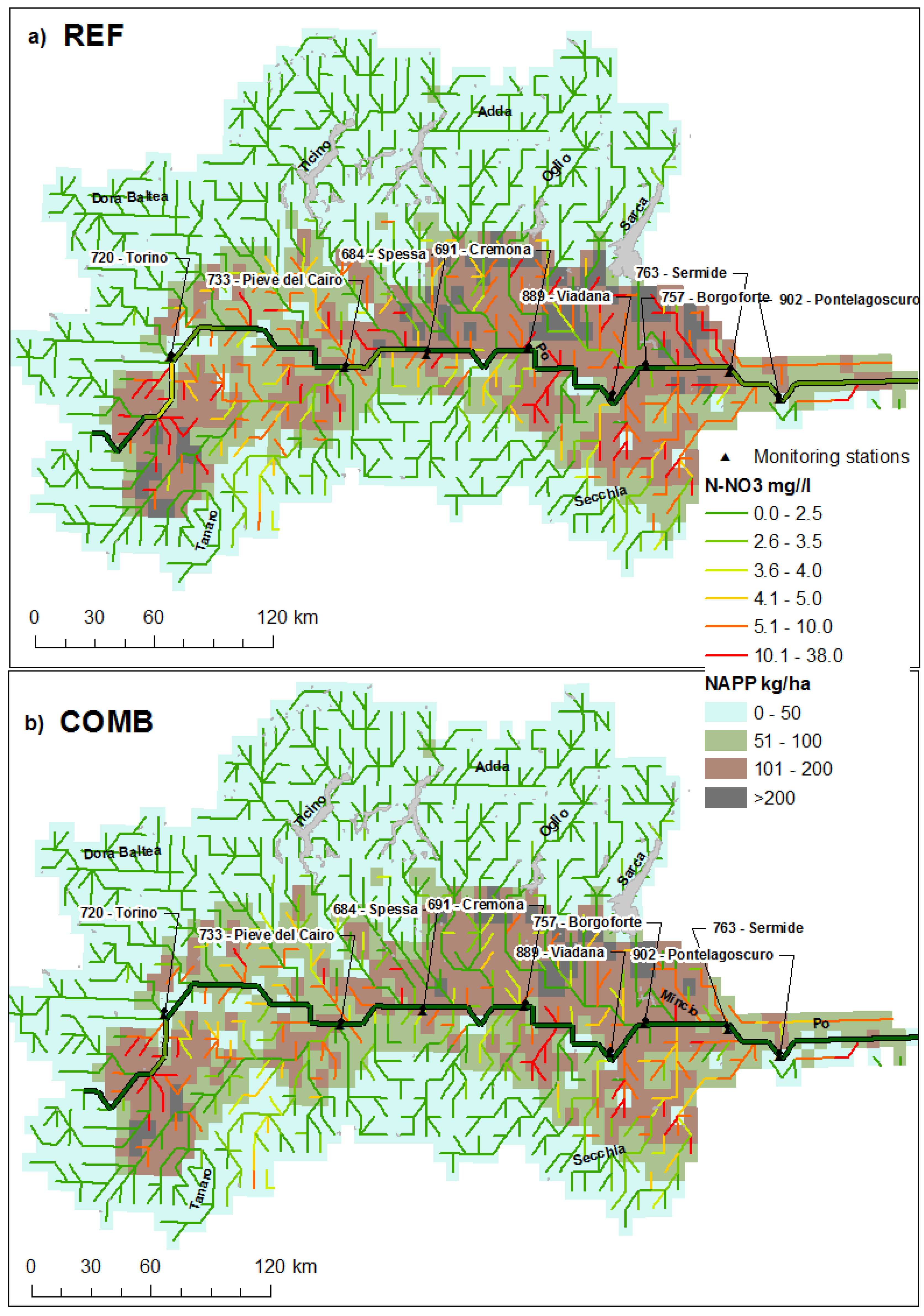
Figure A2.
Spatial distribution of total nitrogen applied (kg/ha) and long term average of annual N-NO3 concentrations (mg/L) in the period 2000–2012 for baseline REF (a) and scenario COMB (b).
Figure A2.
Spatial distribution of total nitrogen applied (kg/ha) and long term average of annual N-NO3 concentrations (mg/L) in the period 2000–2012 for baseline REF (a) and scenario COMB (b).

References
- Beusen, A.H.W.; Bouwman, A.F.; Van Beek, L.P.H.; Mogollón, J.M.; Middelburg, J.J. Global riverine N and P transport to ocean increased during the 20th century despite increased retention along the aquatic continuum. Biogeosciences 2016, 13, 2441–2451. [Google Scholar] [CrossRef]
- Epelde, A.M.; Cerro, I.; Sánchez-Pérez, J.M.; Sauvage, S.; Srinivasan, R.; Antigüedad, I. Application of the SWAT model to assess the impact of changes in agricultural management practices on water quality. Hydrol. Sci. J. 2015, 60, 1–19. [Google Scholar] [CrossRef]
- Liao, L.; Green, C.T.; Bekins, B.A.; Böhlke, J.K. Factors controlling nitrate fluxes in groundwater in agricultural areas. Water Resour. Res. 2012, 48. [Google Scholar] [CrossRef] [Green Version]
- European Commission. Directive 91/676/EEC Concerning the Protection of Waters against Pollution Caused by Nitrates from Agricultural Sources (Nitrates Directive); OJ (1991) L375/1; European Commission: Brussels, Belgium, 1991. [Google Scholar]
- European Commission. Directive 2000/60/EC of the European Parliament and the Council Establishing a Framework for Community Action in the Field of Water Policy (Water Framework Directive); OJ L 327 of 22.12.2000; European Commission: Brussels, Belgium, 2000. [Google Scholar]
- EUROSTAT. Agri-Environmental Indicator—Mineral Fertiliser Consumption-Statistics Explained. Available online: https://ec.europa.eu/eurostat/statistics-explained/index.php/Agri-environmental_indicator_-_mineral_fertiliser_consumption (accessed on 25 March 2019).
- Bouraoui, F.; Grizzetti, B. Modelling mitigation options to reduce diffuse nitrogen water pollution from agriculture. Sci. Total Environ. 2014, 468–469, 1267–1277. [Google Scholar] [CrossRef]
- Jégo, G.; And Martinez, M.; Antiguedad, I.; Launay, M.; Sanchez-Pérez, J.-M. Justes Evaluation of the impact of various agricultural practices on nitrate leaching under the root zone of potato and sugar beet using the STICS soil-crop model. Sci. Total Environ. 2008, 394, 207–221. [Google Scholar]
- Cerro, I.; Antigüedad, I.; Srinavasan, R.; Sauvage, S.; Volk, M.; Sanchez-Perez, J.M. Simulating Land Management Options to Reduce Nitrate Pollution in an Agricultural Watershed Dominated by an Alluvial Aquifer. J. Environ. Qual. 2014, 43, 67. [Google Scholar] [CrossRef]
- Johnes, P.J. Evaluation and management of the impact of land use change on the nitrogen and phosphorus load delivered to surface waters: the export coefficient modelling approach. J. Hydrol. 1996, 183, 323–349. [Google Scholar] [CrossRef]
- Malagó, A.; Bouraoui, F.; Grizzetti, B.; De Roo, A. Modelling nutrient fluxes into the Mediterranean Sea. J. Hydrol. Reg. Stud. 2019, 22, 100592. [Google Scholar] [CrossRef]
- Arnold, J.G.; Srinivasan, R.; Muttiah, R.S.; Williams, J.R. Large area hydrologic modeling and assessment part 1: model development. J. Am. Water Resour. Assoc. 1998, 34, 73–89. [Google Scholar] [CrossRef]
- Borah, D.K.; Bera, M. Watershed-scale hydrologic and nonpoint-source pollution models: review of mathematical bases. Trans. ASAE 2003, 46, 1553–1566. [Google Scholar] [CrossRef]
- Gassman, P.W.; Reyes, M.R.; Green, C.H.; Arnold, J.G.; Gassman, P.W. The Soil and Water Assessment Tool: historical development, applications, and future research directions invited review series. Trans. ASABE 2007, 50, 1211–1250. [Google Scholar] [CrossRef]
- Ferrant, S.; Oehler, F.; Durand, P.; Ruiz, L.; Salmon-Monviola, J.; Justes, E.; Dugast, P.; Probst, A.; Probst, J.-L.; Sanchez-Pérez, J.-M. Understanding nitrogen transfer dynamics in a small agricultural catchment: Comparison of a distributed (TNT2) and a semi distributed (SWAT) modeling approaches. J. Hydrol. 2011, 406, 1–15. [Google Scholar] [CrossRef] [Green Version]
- De Maio, M.; Fiorucci, A.; Offi, M. Risk of groundwater contamination from nitrates in the Po basin (Italy). Water Sci. Technol. Water Supply 2007, 7, 83–92. [Google Scholar] [CrossRef]
- Montanari, A. Hydrology of the Po River: looking for changing patterns in river discharge. Hydrol. Earth Syst. Sci 2012, 16, 3739–3747. [Google Scholar] [CrossRef]
- Lasagna, M.; De Luca, D.A. Evaluation of sources and fate of nitrates in the western Po plain groundwater (Italy) using nitrogen and boron isotopes. Environ. Sci. Pollut. Res. 2019, 26, 2089–2104. [Google Scholar] [CrossRef]
- Palmeri, L.; Bendoricchio, G.; Artioli, Y. Modelling nutrient emissions from river systems and loads to the coastal zone: Po River case study, Italy. Ecol. Modell. 2005, 184, 37–53. [Google Scholar] [CrossRef]
- Salvetti, R.; Azzellino, A.; Vismara, R. Diffuse source apportionment of the Po river eutrophying load to the Adriatic sea: Assessment of Lombardy contribution to Po river nutrient load apportionment by means of an integrated modelling approach. Chemosphere 2006, 65, 2168–2177. [Google Scholar] [CrossRef]
- Malagó, A.; Pagliero, L.; Bouraoui, F.; Franchini, M. Comparing calibrated parameter sets of the SWAT model for the Scandinavian and Iberian peninsulas. Hydrol. Sci. J. 2015, 60, 949–967. [Google Scholar] [CrossRef]
- Malagó, A.; Bouraoui, F.; Vigiak, O.; Grizzetti, B.; Pastori, M. Modelling water and nutrient fluxes in the Danube River Basin with SWAT. Sci. Total Environ. 2017, 603–604, 196–218. [Google Scholar] [CrossRef]
- Pagliero, L.; Bouraoui, F.; Willems, P.; Diels, J. Large-Scale Hydrological Simulations Using the Soil Water Assessment Tool, Protocol Development, and Application in the Danube Basin. J. Environ. Qual. 2014, 43, 145. [Google Scholar] [CrossRef] [Green Version]
- Arnold, J.G.; Moriasi, D.N.; Gassman, P.W.; Abbaspour, K.C.; White, M.J.; Srinivasan, R.; Santhi, C.; Harmel, R.D.; van Griensven, A.; Liew, M.W.V.; et al. SWAT: Model Use, Calibration, and Validation. Trans. ASABE 2012, 55, 1491–1508. [Google Scholar] [CrossRef]
- Neitsch, S.L.; Arnold, J.G.; Kiniry, J.R.; Williams, J.R. Soil and Water Assessment Tool Theoretical Documentation Version 2009; Texas Water Resources Institute: College Station, TX, USA, 2011. [Google Scholar]
- Rathjens, H.; Oppelt, N. SWATgrid: An interface for setting up SWAT in a grid-based discretization scheme. Comput. Geosci. 2012, 45, 161–167. [Google Scholar] [CrossRef]
- LP DAAC Global 30 Arc-Second Elevation Data Set GTOPO30. Land Process Distributed Active Archive Center. Available online: https://www.usgs.gov (accessed on 10 October 2016).
- Arino, O.; Perez, R.J.J.; Kalogirou, V.; Bontemps, S.; Defourny, P.; Van Bogaert, E. Global Land Cover Map for 2009 (GlobCover 2009). PANGAEA 2012. [Google Scholar] [CrossRef]
- You, L.; Wood-Sichra, U.; Fritz, S.; Guo, Z.; See, L.; Koo, J. Spatial Production Allocation Model (SPAM) 2005 v2.0. 2014. Available online: http://mapspam.info (accessed on 1 September 2016).
- Harmonized World Soil Database (Version 1.2); FAO: Rome, Italy; IIASA: Laxenburg, Austria; ISRIC: Wageningen, The Netherlands; ISSCAS: Nanjing, China; JRC: Brussels, Belgium, 2012.
- Rawls, W.J.; Brakensiek, D.L. Prediction of soil water properties for hydrologic modeling. In Proceedings of the Symposium of Watershed Management in the Eighties, Denver, CO, USA, 30 April–1 May 2016; Jones, E.B., Ward, T.J., Eds.; American Society of Civil Engineers: New York, NY, USA, 1985; pp. 293–299. [Google Scholar]
- Saxton, K.E.; Rawls, W.J. Soil Water Characteristic Estimates by Texture and Organic Matter for Hydrologic Solutions. Soil Sci. Soc. Am. J. 2006, 70, 1569–1578. [Google Scholar] [CrossRef]
- Messager, M.L.; Lehner, B.; Grill, G.; Nedeva, I.; Schmitt, O. Estimating the volume and age of water stored in global lakes using a geo-statistical approach. Nat. Commun. 2016, 7, 13603. [Google Scholar] [CrossRef] [Green Version]
- Beck, H.E.; Vergopolan, N.; Pan, M.; Levizzani, V.; Van Dijk, A.I.J.M.; Weedon, G.P.; Brocca, L.; Pappenberger, F.; Huffman, G.J.; Wood, E.F. Global-scale evaluation of 22 precipitation datasets using gauge observations and hydrological modeling. Hydrol. Earth Syst. Sci. 2017, 21, 6201–6217. [Google Scholar] [CrossRef] [Green Version]
- Dee, D.P.; Uppala, S.M.; Simmons, A.J.; Berrisford, P.; Poli, P.; Kobayashi, S.; Andrae, U.; Balmaseda, M.A.; Balsamo, G.; Bauer, P.; et al. The ERA-Interim reanalysis: configuration and performance of the data assimilation system. Q. J. R. Meteorol. Soc. 2011, 137, 553–597. [Google Scholar] [CrossRef] [Green Version]
- Huang, Z.; Hejazi, M.; Li, X.; Tang, Q.; Vernon, C.; Leng, G.; Liu, Y.; Döll, P.; Eisner, S.; Gerten, D.; et al. Reconstruction of global gridded monthly sectoral water withdrawals for 1971–2010 and analysis of their spatiotemporal patterns. Hydrol. Earth Syst. Sci. 2018, 22, 2117–2133. [Google Scholar] [CrossRef]
- Portmann, F.T.; Siebert, S.; Döll, P. MIRCA2000-Global monthly irrigated and rainfed crop areas around the year 2000: A new high-resolution data set for agricultural and hydrological modeling. Global Biogeochem. Cycles 2010, 24. [Google Scholar] [CrossRef] [Green Version]
- Siebert, S.; Döll, P. Quantifying blue and green virtual water contents in global crop production as well as potential production losses without irrigation. J. Hydrol. 2010, 384, 198–217. [Google Scholar] [CrossRef]
- Franke, G.R. Stepwise Regression. In Wiley International Encyclopedia of Marketing; John Wiley & Sons, Ltd.: Chichester, UK, 2010; ISBN 9781444316568. [Google Scholar]
- Daggupati, P.; Yen, H.; White, M.J.; Srinivasan, R.; Arnold, J.G.; Keitzer, C.S.; Sowa, S.P. Impact of model development, calibration and validation decisions on hydrological simulations in West Lake Erie Basin. Hydrol. Process. 2015, 29, 5307–5320. [Google Scholar] [CrossRef]
- Moriasi, D.N.; Arnold, J.G.; Van Liew, M.W.; Bingner, R.L.; Harmel, R.D.; Veith, T.L. Model evaluation guidelines for systematic quantification of accuracy in watershed simulations. Trans. ASABE 2007, 50, 885–900. [Google Scholar] [CrossRef]
- Zambrano-Bigiarini, M. hydroGOF: Goodness-of-fit Functions for Comparison of Simulated and Observed Hydrological Time SeriesR Package Version 0.3-10. Available online: https://cran.r-project.org/web/packages/hydroGOF/hydroGOF.pdf (accessed on 10 October 2016).
- FAOSTAT. 2018. Available online: http://www.fao.org/faostat/en/#data/QC (accessed on 26 March 2019).
- Williams, J.R. Chapter 25: The EPIC Model. In: Computer models of watershed hydrology. Water Resour. Publ. 1995, 909–1000. [Google Scholar]
- Yang, M.; Xiao, W.; Zhao, Y.; Li, X.; Huang, Y.; Lu, F.; Hou, B.; Li, B.; Yang, M.; Xiao, W.; et al. Assessment of Potential Climate Change Effects on the Rice Yield and Water Footprint in the Nanliujiang Catchment, China. Sustainability 2018, 10, 242. [Google Scholar] [CrossRef]
- Abbaspour, K.C. User Manual for SWAT-CUP, SWAT Calibration, and Uncertainty Analysis Programs; Swiss Federal Institute of Aquatic Science and Technology Eawag: Duebendorf, Switzerland, 2012. [Google Scholar]
- Pagliero, L.; Bouraoui, F.; Diels, J.; Willems, P.; McIntyre, N. Investigating regionalization techniques for large-scale hydrological modelling. J. Hydrol. 2019, 570, 220–235. [Google Scholar] [CrossRef]
- Kohonen, T. Essentials of the self-organizing map. Neural Netw. 2013, 37, 52–65. [Google Scholar] [CrossRef]
- Malagó, A.; Vigiak, O.; Bouraoui, F.; Pagliero, L.; Franchini, M. The Hillslope Length Impact on SWAT Streamflow Prediction in Large Basins. J. Environ. Inform. 2018, 32, 82–97. [Google Scholar] [CrossRef]
- Nakagawa, A.; Kutics, A. Classification in Big Image Datasets Using Layered-SOM. In Proceedings of the 13th International Conference on Signal-Image Technology & Internet-Based Systems (SITIS), Jaipur, India, 4–7 December 2017; pp. 143–150. [Google Scholar]
- Ward, J.H. Hierarchical Grouping to Optimize an Objective Function. J. Am. Stat. Assoc. 1963, 58, 236–244. [Google Scholar] [CrossRef] [Green Version]
- Charrad, M.; Ghazzali, N.; Boiteau, V.; Niknafs, A. NbClust: An R Package for Determining the Relevant Number of Clusters in a Data Set. J. Stat. Softw. 2014, 61, 1–36. [Google Scholar] [CrossRef]
- Motsinger, J.; Kalita, P.; Bhattarai, R.; Motsinger, J.; Kalita, P.; Bhattarai, R. Analysis of Best Management Practices Implementation on Water Quality Using the Soil and Water Assessment Tool. Water 2016, 8, 145. [Google Scholar] [CrossRef]
- Meyer, N.; Bergez, J.-E.; Constantin, J.; Justes, E. Cover crops reduce water drainage in temperate climates: A meta-analysis. Agron. Sustain. Dev. 2019, 39, 3. [Google Scholar] [CrossRef]
- Naldi, M.; Pierobon, E.; Tornatore, F.; Viaroli, P. Il ruolo degli eventi di piena nella formazione e distribuzione temporale dei carichi di fosforo e azoto nel fiume Po. Atti XVIII Congr. S.It.E 2005, 24, 59–69. [Google Scholar]
- Yeo, I.-Y.; Lee, S.; Sadeghi, A.M.; Beeson, P.C.; Hively, W.D.; Mccarty, G.W.; Lang, M.W. Assessing winter cover crop nutrient uptake efficiency using a water quality simulation model. Hydrol. Earth Syst. Sci 2014, 18, 5239–5253. [Google Scholar] [CrossRef] [Green Version]
- Kaspar, T.C.; Jaynes, D.B.; Parkin, T.B.; Moorman, T.B. Rye Cover Crop and Gamagrass Strip Effects on NO Concentration and Load in Tile Drainage. J. Environ. Qual. 2007, 36, 1503. [Google Scholar] [CrossRef]
- Islam, N.; Wallender, W.W.; Mitchell, J.; Wicks, S.; Howitt, R.E. A comprehensive experimental study with mathematical modeling to investigate the affects of cropping practices on water balance variables. Agric. Water Manag. 2006, 82, 129–147. [Google Scholar] [CrossRef]
- Marcillo, G.S.; Miguez, F.E. Corn yield response to winter cover crops: An updated meta-analysis. J. Soil Water Conserv. 2017, 72, 226–239. [Google Scholar] [CrossRef]
- Lasagna, M.; De Luca, D.A.; Franchino, E. Nitrate contamination of groundwater in the western Po Plain (Italy): the effects of groundwater and surface water interactions. Environ. Earth Sci. 2016, 75, 240. [Google Scholar] [CrossRef]
- Bartoli, M.; Racchetti, E.; Delconte, C.A.; Sacchi, E.; Soana, E.; Laini, A.; Longhi, D.; Viaroli, P. Nitrogen balance and fate in a heavily impacted watershed (Oglio River, Northern Italy): in quest of the missing sources and sinks. Biogeosciences 2012, 9, 361–373. [Google Scholar] [CrossRef] [Green Version]
- Spillman, C.M.; Imberger, J.; Hamilton, D.P.; Hipsey, M.R.; Romero, J.R. Modelling the effects of Po River discharge, internal nutrient cycling and hydrodynamics on biogeochemistry of the Northern Adriatic Sea. J. Mar. Syst. 2007, 68, 167–200. [Google Scholar] [CrossRef]
- Rittenburg, R.A.; Squires, A.L.; Boll, J.; Brooks, E.S.; Easton, Z.M.; Steenhuis, T.S. Agricultural BMP Effectiveness and Dominant Hydrological Flow Paths: Concepts and a Review. JAWRA J. Am. Water Resour. Assoc. 2015, 51, 305–329. [Google Scholar] [CrossRef]
- Teshager, A.D.; Gassman, P.W.; Secchi, S.; Schoof, J.T. Simulation of targeted pollutant-mitigation-strategies to reduce nitrate and sediment hotspots in agricultural watershed. Sci. Total Environ. 2017, 607–608, 1188–1200. [Google Scholar] [CrossRef] [PubMed]
- De Wit, M.; Behrendt, H.; Bendoricchio, G.; Bleuten, W.; Van Gaans, P. The contribution of agriculture to nutrient pollution in three European rivers, with reference to the European Nitrates Directive. Eur. Water Manag. 2002. Available online: http://www.ewa-online.eu/tl_files/_media/content/documents_pdf/Publications/E-WAter/documents/90_2002_02.pdf (accessed on 13 November 2018).
- Martinez, J.; Burton, C. Manure Management and Treatment: An Overview of the European Situation; International Conference of Animal Hygiene: Mexico, 2003; Available online: https://www.isah-soc.org/userfiles/downloads/proceedings/2003/mainspeakers/15MartinezFrance.pdf (accessed on 13 November 2018).
- Vezzoli, R.; Mercogliano, P.; Pecora, S.; Zollo, A.L.; Cacciamani, C. Hydrological simulation of Po River (North Italy) discharge under climate change scenarios using the RCM COSMO-CLM. Sci. Total Environ. 2015, 521–522, 346–358. [Google Scholar] [CrossRef] [PubMed]
Figure 1.
Map of the Po River Basin with the main hydrographic network, regions border and monitoring stations used in this study (a). SWAT model discretization of the Po River Basin (b).
Figure 1.
Map of the Po River Basin with the main hydrographic network, regions border and monitoring stations used in this study (a). SWAT model discretization of the Po River Basin (b).

Figure 2.
Comparison of simulated and observed annual crop yields from SPAM (a) and FAOSTAT (b) in the period 2000–2012. The acronyms of crop names are reported in Table A1 in Appendix A.
Figure 2.
Comparison of simulated and observed annual crop yields from SPAM (a) and FAOSTAT (b) in the period 2000–2012. The acronyms of crop names are reported in Table A1 in Appendix A.

Figure 3.
Comparison of simulated (SIM) and observed (OBS) monthly streamflow (m3/s), N-NO3 concentrations (mg/L) and loads (kg/month) in the calibration (CAL, upper three graphs) and validation (VAL, lower three graphs) periods.
Figure 3.
Comparison of simulated (SIM) and observed (OBS) monthly streamflow (m3/s), N-NO3 concentrations (mg/L) and loads (kg/month) in the calibration (CAL, upper three graphs) and validation (VAL, lower three graphs) periods.

Figure 4.
Monthly time series of streamflow (a,d), nitrogen-nitrate concentrations (b,e) and monthly loads (c,f) observed (red lines and points) and simulated by SWAT (black line) at two selected gauging stations across the Po River.
Figure 4.
Monthly time series of streamflow (a,d), nitrogen-nitrate concentrations (b,e) and monthly loads (c,f) observed (red lines and points) and simulated by SWAT (black line) at two selected gauging stations across the Po River.

Figure 5.
Box plots of residuals (simulation-observation) of monthly streamflow (a), N-NO3 concentrations (b), loads (c) and specific loads (d) along 6 stations from source to mouth (left to right) of the Po River.
Figure 5.
Box plots of residuals (simulation-observation) of monthly streamflow (a), N-NO3 concentrations (b), loads (c) and specific loads (d) along 6 stations from source to mouth (left to right) of the Po River.

Figure 6.
Long-term mean annual water, mm, (a) and nitrogen, kg/ha, (b) balances for the entire Po River Basin for the period 2000–2012. In (a): PCP precipitation, ET evapotranspiration, INF infiltration, SR surface runoff, LF lateral flow, BFS groundwater from shallow aquifer, BFD groundwater from deep aquifer. In (b): NAPP nitrogen applied as fertilizer, NMIN nitrogen mineral fertilizer, NMAN nitrogen manure fertilizer, NFIX nitrogen fixation, NRAIN nitrogen in atmospheric deposition, Nyld nitrogen removed by crop yields, SRN nitrogen transported via surface runoff, LFN nitrogen transported via lateral flow, ORGN organic nitrogen transported with sediment, BFN nitrogen transported via groundwater, Nleach nitrates that leached into aquifer, NPS nitrogen from point sources directly discharged into rivers, Nloads nitrogen loads into rivers.

Figure 7.
Changing of total nitrogen applied as fertilizer, crop yields, and nitrogen leaching for four dominant crops in the basin per scenarios (LMAI: low intensive corn, IMAI: irrigated corn, HWHE: highly intensive wheat, IRIC: irrigated rice).
Figure 7.
Changing of total nitrogen applied as fertilizer, crop yields, and nitrogen leaching for four dominant crops in the basin per scenarios (LMAI: low intensive corn, IMAI: irrigated corn, HWHE: highly intensive wheat, IRIC: irrigated rice).

Figure 8.
Spatial analysis of distribution of long-term mean of nitrogen emissions (kg/ha), nitrogen leached into aquifer (kg/ha) and nitrate concentration leached into aquifer for the baseline (REF) and scenarios NMIN, MAN170, CRP3 and COMB.
Figure 8.
Spatial analysis of distribution of long-term mean of nitrogen emissions (kg/ha), nitrogen leached into aquifer (kg/ha) and nitrate concentration leached into aquifer for the baseline (REF) and scenarios NMIN, MAN170, CRP3 and COMB.

Figure 9.
Comparison of simulated long-term mean annual N-NO3 concentrations and loads in the period 2003–2008 (where observations are concentrated) as function of the distance from the mouth. The black dots represent the long term mean annual observations calculated in the period 2003–2008.
Figure 9.
Comparison of simulated long-term mean annual N-NO3 concentrations and loads in the period 2003–2008 (where observations are concentrated) as function of the distance from the mouth. The black dots represent the long term mean annual observations calculated in the period 2003–2008.

Table 1.
Land cover classes distribution in the Po River Basin.
| Land Use | Area (km2) | Percentage (%) |
|---|---|---|
| Bare | 804 | 1% |
| Fodder crops | 12,848 | 17% |
| Forest | 25,133 | 34% |
| Irrigated crops | 4337 | 6% |
| Managed grassland | 18,943 | 25% |
| Rainfed crops | 7707 | 10% |
| Shrub | 350 | 0% |
| Urban area | 3297 | 4% |
| Water | 1171 | 2% |
| Total | 74,590 | 100% |
Table 2.
Example of management operations for irrigated corn (grid-cell 403, HRU 5) as defined in SWAT for baseline and scenario CRP2 (see Section 2.4).
Table 2.
Example of management operations for irrigated corn (grid-cell 403, HRU 5) as defined in SWAT for baseline and scenario CRP2 (see Section 2.4).
| Scenario | Operation Code | Description | Month | Day | Application |
|---|---|---|---|---|---|
| Baseline | FERT MANN | Amount of N manure fertilizer application (0.99 ORGN) | 10 | 14 | 112.2 kg/ha |
| FERT MANP | Amount of P manure fertilizer application (0.99 ORGP) | 10 | 14 | 24.7 kg/ha | |
| TILLAGE1 | Disk Chisel (mulch Tiller) with depth of 150 mm and mixing efficiency of 0.55 | 10 | 15 | ||
| TILLAGE2 | Harrow 10 Bar Tine 36 Ft with depth of 25 mm and mixing efficiency of 0.2 | 10 | 24 | ||
| PLANTING CORN | Beginning of plant growth | 4 | 1 | 1787 HU | |
| FERT MINN | Amount of elemental N fertilizer applied to HRU | 4 | 11 | 221.6 kg/ha | |
| FERT MINP | Amount of elemental P fertilizer applied to HRU | 4 | 11 | 34.7 kg/ha | |
| IRRIGATION 1 | Depth of irrigation water applied on HRU | 4 | 22 | 12.6 mm | |
| IRRIGATION 2 | Depth of irrigation water applied on HRU | 5 | 7 | 12.6 mm | |
| IRRIGATION 3 | Depth of irrigation water applied on HRU | 5 | 22 | 12.6 mm | |
| IRRIGATION 4 | Depth of irrigation water applied on HRU | 6 | 6 | 12.6 mm | |
| IRRIGATION 5 | Depth of irrigation water applied on HRU | 6 | 21 | 12.6 mm | |
| IRRIGATION 6 | Depth of irrigation water applied on HRU | 7 | 6 | 12.6 mm | |
| IRRIGATION 7 | Depth of irrigation water applied on HRU | 7 | 21 | 12.6 mm | |
| IRRIGATION 8 | Depth of irrigation water applied on HRU | 8 | 5 | 12.6 mm | |
| IRRIGATION 9 | Depth of irrigation water applied on HRU | 8 | 11 | 12.6 mm | |
| IRRIGATION 10 | Depth of irrigation water applied on HRU | 8 | 17 | 12.6 mm | |
| HARVEST and KILL of CORN | Harvest and kill operation stops the plant growth in the HRU | 9 | 1 | ||
| CRP2 | HARVEST and KILL RYE | Harvest and kill operation stops the plant growth in the HRU | 3 | 15 | |
| FERT MANN | Amount of N manure fertilizer application (0.99 ORGN) | 3 | 20 | 112.2 kg/ha | |
| FERT MANP | Amount of P manure fertilizer application (0.99 ORGP) | 3 | 20 | 24.7 kg/ha | |
| PLANTING CORN | Beginning of plant growth | 4 | 1 | 1787 HU | |
| FERT MINN | Amount of elemental N fertilizer applied to HRU | 4 | 11 | 199.5 kg/ha | |
| FERT MINP | Amount of elemental P fertilizer applied to HRU | 4 | 11 | 34.7 kg/ha | |
| IRRIGATION 1 | Depth of irrigation water applied on HRU | 4 | 22 | 12.6 mm | |
| IRRIGATION 2 | Depth of irrigation water applied on HRU | 5 | 7 | 12.6 mm | |
| IRRIGATION 3 | Depth of irrigation water applied on HRU | 5 | 22 | 12.6 mm | |
| IRRIGATION 4 | Depth of irrigation water applied on HRU | 6 | 6 | 12.6 mm | |
| IRRIGATION 5 | Depth of irrigation water applied on HRU | 6 | 21 | 12.6 mm | |
| IRRIGATION 6 | Depth of irrigation water applied on HRU | 7 | 6 | 12.6 mm | |
| IRRIGATION 7 | Depth of irrigation water applied on HRU | 7 | 21 | 12.6 mm | |
| IRRIGATION 8 | Depth of irrigation water applied on HRU | 8 | 5 | 12.6 mm | |
| IRRIGATION 9 | Depth of irrigation water applied on HRU | 8 | 11 | 12.6 mm | |
| IRRIGATION 10 | Depth of irrigation water applied on HRU | 8 | 17 | 12.6 mm | |
| HARVEST and KILL of CORN | Harvest and kill operation stops the plant growth in the HRU | 9 | 1 | ||
| TILLAGE2 | Harrow 10 Bar Tine 36 Ft with depth of 25 mm and mixing efficiency of 0.2 | 9 | 3 | ||
| PLANTING RYE | The initiation of plant growth | 9 | 4 | 800 HU |
Table 3.
Characterization of monitoring stations along the Po River (# is the number of data entries).
Table 3.
Characterization of monitoring stations along the Po River (# is the number of data entries).
| ID | Description | Drained Area (km2) | Distance from the Source (km) | # Data Entries for Streamflow (2000–2012) | # Data Entries for N-NO3 (2000–2012) |
|---|---|---|---|---|---|
| 720 | Po at Torino | 7193 | 462 | 60 | |
| 733 | Po at Pieve del Cairo | 26,467 | 355 | 108 | 33 |
| 684 | Po at Spessa | 38,468 | 303 | 108 | 55 |
| 691 | Po at Cremona Castelvetro | 51,337 | 247 | 144 | 63 |
| 889 | Po at Viadana | 56,350 | 172 | 108 | 62 |
| 757 | Po at Borgoforte | 63,765 | 147 | 108 | 59 |
| 763 | Po at Sermide | 70,007 | 101 | 108 | 61 |
| 902 | Po at Pontelagoscuro | 72,396 | 65 | 144 |
Table 4.
Description of calibrated parameters involved in the calibration with their range before and after calibration.
Table 4.
Description of calibrated parameters involved in the calibration with their range before and after calibration.
| Process | Parameter and Input File | HRUs | Description | Range | Calibrated Value |
|---|---|---|---|---|---|
| Plant growth | T_Base.crop | Bare, shrub and grassland | Minimum/base temperature for plant growth | 0.12 | 1 |
| Fodder crop | Minimum/base temperature for plant growth | 0–12 | 3 | ||
| BIO_E.crop | Fodder crop | Radiation use efficiency | 10–90 | 5 | |
| Irrigated sugar beet | Radiation use efficiency | 10–90 | 20 | ||
| Rice | Radiation use efficiency | 10–90 | 25 | ||
| HVSTI.crop | Rice | Harvest index | 0.01–1.25 | 0.54 | |
| FRGRW2.crop | Rice | Fraction of the plant growing season corresponding to the 2nd point on the optimal leaf area development curve | 0–1 | 0.51 | |
| LAIMX1.crop | Rice | Fraction of the maximum leaf area index corresponding to the 1st point on the optimal leaf area development curve | 0–1 | 0.28 | |
| LAIMX2.crop | Rice | Fraction of the maximum leaf area index corresponding to the 2nd point on the optimal leaf area development curve | 0–1 | 0.99 | |
| Baseflow generation | ALPHA_BF.gw | all | Baseflow alpha factor | −0.5–0.5 (relative) | 0.045 (relative) 1 |
| GW_DELAY.gw | all | Groundwater delay time | −0.5–0.5 (relative) | −0.497 (relative) | |
| RCHRG_DP.gw | all | Deep aquifer percolation fraction | −0.5–0.5 (relative) | 0.377 (relative) | |
| Nitrogen cycle | HLIFE_NGW.gw | all | Half-life of the nitrate in shallow aquifer | 100–1000 | 1007.5 |
| CMN.bsn | all | Rate factor for humus mineralization of active organic nutrients | 0.0001–0.003 | 0.001465 |
1 “relative” means that the existing value is multiplied by (1 + the given value).
Table 5.
Scenario descriptions (# is the number of HRUs).
| Scenario Acronym | Description | #HRU Affected | Area (km2) |
|---|---|---|---|
| NMIN | Strategic reduction of mineral fertilizer application in each HRU limiting the change in annual crop yield from baseline below 5% | 2208 | 12044 |
| MAN170 | Restriction of manure application to maximum 170 kg N/ha/y | 71 | 332 |
| MAN250 | Restriction of manure application to maximum 250 kg N/ha/y | 9 | 40 |
| CRP1 | Planting rye after harvesting corn and harvesting it before planting corn. | 730 | 5503 |
| CRP2 | Strategic reduction of mineral fertilizer application in each HRU with corn (as scenario NMIN) and planting rye as cover crop (as scenario CRP1) after harvesting corn | 730 | 5503 |
| CRP3 | Strategic reduction of mineral fertilizer application in each HRU with corn (as scenario NMIN) and planting red clover as cover crop after harvesting corn | 730 | 5503 |
| COMB | Combination of scenario NMIN, MAN170 and CRP3 | 2208 | 12044 |
Table 6.
Pearson correlation coefficient (r) calculated between SWAT simulated annual crop yields and FAOSTAT in the period 2000-2012 for the main crops in the basin.
Table 6.
Pearson correlation coefficient (r) calculated between SWAT simulated annual crop yields and FAOSTAT in the period 2000-2012 for the main crops in the basin.
| Crop Code | Crop Name | Area (ha) | r |
|---|---|---|---|
| LMAI | Corn under low intensive management | 3717 | 0.58 |
| IMAI | Irrigated corn | 1782 | 0.70 |
| HWHE | Wheat under highly intensive management | 1748 | −0.06 |
| IRIC | Irrigated rice | 1740 | −0.60 |
Table 7.
Description of calibrated and validated variables (# = number; N-NO3 = nitrogen nitrates) and model performance.
Table 7.
Description of calibrated and validated variables (# = number; N-NO3 = nitrogen nitrates) and model performance.
| Variable | # Monitoring Stations/Data Entries | Simulation Period | PBIAS (%) |
|---|---|---|---|
| Monthly streamflow | 8/408 | Calibration (2005–2012) | 3.7 |
| 8/480 | Validation (2000–2004) | −10.8 | |
| Monthly N-NO3 concentrations | 6/244 | Calibration (2005–2012) | 12 |
| 6/89 | Validation (2000–2004) | −4.1 | |
| Monthly N-NO3 loads | 6/244 | Calibration (2005–2012) | 14.1 |
| 6/89 | Validation (2000–2004) | −19.4 | |
| 6/333 | Evaluation (2000–2012) | 4.3 |
Table 8.
Comparison N-NO3 SWAT annual estimations at Pontelagoscuro with other studies and observations at Sermide, the nearest station to Pontelagoscuro with observations.
Table 8.
Comparison N-NO3 SWAT annual estimations at Pontelagoscuro with other studies and observations at Sermide, the nearest station to Pontelagoscuro with observations.
| Reference | Model | Period | N-NO3 (ton/y) |
|---|---|---|---|
| Our study | SWAT | 2000–2012 | 115,000 |
| 2003–2008 | 93,460 | ||
| 2003–2007 | 78,032 | ||
| Salvetti et al. [20] | QUAL2E/SWAT | 1985–2001 | 107,000 |
| Palmeri et al. [19] | MONERIS | 1996–2000 | 123,482 * |
| Naldi et al. [55] | - | 2003–2007 | 85,000 |
| Malagó et al. [11] | GREEN-Rgrid | 2003–2007 | 86,295 |
| Long term average annual load at Sermide | - | 2003–2008 | 93,462 |
* DIN dissolved inorganic nitrogen.
Table 9.
Specific nutrient loads per scenarios in cropland HRUs (12,044 km2, 16% of the whole basin). In parenthesis the percentage of reduction (negative values) or increment (positive values) respect the baseline (REF).
Table 9.
Specific nutrient loads per scenarios in cropland HRUs (12,044 km2, 16% of the whole basin). In parenthesis the percentage of reduction (negative values) or increment (positive values) respect the baseline (REF).
| Scenarios | |||||||||||||||||
|---|---|---|---|---|---|---|---|---|---|---|---|---|---|---|---|---|---|
| Components | Units of Measures | REF | NMIN | NMAN170 | NMAN250 | CRP1 | CRP2 | CRP3 | COMB | ||||||||
| NAPP | Mineral fertilizer and manure application | kg N/ha | 199.28 | 165.23 | (−17%) | 198.28 | (−1%) | 199.18 | (0%) | 199.28 | (0%) | 184.2 | (−8%) | 184.2 | (−8%) | 164.24 | (−18%) |
| NMIN | Mineral fertilizer | kg N/ha | 149.07 | 115.03 | (−23%) | 149.07 | (0%) | 149.07 | (0%) | 149.07 | (0%) | 134 | (−10%) | 134 | (−10%) | 115.03 | (−23%) |
| NMAN | Manure | kg N/ha | 50.2 | 50.2 | (0%) | 49.2 | (−2%) | 50.1 | (0%) | 50.2 | (0%) | 50.2 | (0%) | 50.2 | (0%) | 49.2 | (−2%) |
| NFIX | Nitrogen fixation | kg N/ha | 3.21 | 3.21 | (0%) | 3.23 | (1%) | 3.21 | (0%) | 3.21 | (0%) | 3.21 | (0%) | 21.49 | (569%) | 21.66 | (575%) |
| NRAIN | Nitrogen in atmospheric deposition | kg N/ha | 13.4 | 13.4 | (0%) | 13.4 | (0%) | 13.4 | (0%) | 13.4 | (0%) | 13.4 | (0%) | 13.4 | (0%) | 13.4 | (0%) |
| NUP 1 | Nitrogen uptake in the soil | kg N/ha | 185.38 | 166.29 | (−10%) | 185.19 | (0%) | 185.37 | (0%) | 209.07 | (13%) | 193.89 | (5%) | 217.28 | (17%) | 210.99 | (14%) |
| Nleach | NO3 leached into the aquifer | kg N/ha | 125.4 | 95.47 | (−24%) | 124.71 | (−1%) | 125.33 | (0%) | 109.65 | (−13%) | 98.83 | (−21%) | 97.19 | (−22%) | 78.63 | (−37%) |
| Nem | Nitrogen emissions | kg N/ha | 66.51 | 52.64 | (−21%) | 66.25 | (0%) | 66.48 | (0%) | 55.86 | (−16%) | 51.59 | (−22%) | 50.7 | (−24%) | 41.7 | (−37%) |
| SRN | Nitrogen transported via surface runoff | kg N/ha | 1.24 | 1.08 | (−13%) | 1.24 | (0%) | 1.24 | (0%) | 1.24 | (0%) | 1.13 | (−9%) | 1.16 | (−6%) | 1.09 | (−12%) |
| LFN | Nitrogen transported via lateral flow | kg N/ha | 0.07 | 0.06 | (−14%) | 0.07 | (0%) | 0.07 | (0%) | 0.06 | (−14%) | 0.06 | (−14%) | 0.06 | (−14%) | 0.05 | (−29%) |
| ORGN | Organic nitrogen transported with sediment | kg N/ha | 9.57 | 9.2 | (−4%) | 9.55 | (0%) | 9.57 | (0%) | 6.39 | (−33%) | 6.2 | (−35%) | 5.78 | (−40%) | 5.68 | (−41%) |
| BFN | NO3 transported via groundwater | kg N/ha | 55.63 | 42.3 | (−24%) | 55.39 | (0%) | 55.6 | (0%) | 48.17 | (−13%) | 44.2 | (−21%) | 43.7 | (−21%) | 34.88 | (−37%) |
| SYLD | Sediment yield | ton/y | 6.25 | 6.26 | (0%) | 6.25 | (0%) | 6.25 | (0%) | 3.03 | (−52%) | 3.04 | (−51%) | 2.93 | (−53%) | 2.93 | (−53%) |
| YLD | Crop yield | ton/y | 5.97 | 5.78 | (−3%) | 5.96 | (0%) | 5.96 | (0%) | 6.53 | (9%) | 6.39 | (7%) | 7.07 | (18%) | 7.01 | (17%) |
1 Plant uptake of N in the soil. This is the result of the processes involved in the nitrogen cycle in the soil (mineralization, decomposition, nitrification, ammonia volatilization and denitrification). Instead, Nyld (Figure 6) is the nitrogen removed with the crop yields, thus it represents the effective amount of nitrogen losses from the system by plants.
© 2019 by the authors. Licensee MDPI, Basel, Switzerland. This article is an open access article distributed under the terms and conditions of the Creative Commons Attribution (CC BY) license (http://creativecommons.org/licenses/by/4.0/).
Share and Cite
MDPI and ACS Style
Malagó, A.; Bouraoui, F.; Pastori, M.; Gelati, E. Modelling Nitrate Reduction Strategies from Diffuse Sources in the Po River Basin. Water 2019, 11, 1030. https://doi.org/10.3390/w11051030
AMA Style
Malagó A, Bouraoui F, Pastori M, Gelati E. Modelling Nitrate Reduction Strategies from Diffuse Sources in the Po River Basin. Water. 2019; 11(5):1030. https://doi.org/10.3390/w11051030
Chicago/Turabian StyleMalagó, Anna, Fayçal Bouraoui, Marco Pastori, and Emiliano Gelati. 2019. "Modelling Nitrate Reduction Strategies from Diffuse Sources in the Po River Basin" Water 11, no. 5: 1030. https://doi.org/10.3390/w11051030
Note that from the first issue of 2016, this journal uses article numbers instead of page numbers. See further details here.