Susceptibility of Hydropower Generation to Climate Change: Karun III Dam Case Study


1
Department of Civil and Environmental Engineering, Norwegian University of Science and Technology (NTNU), N7491 Trondheim, Norway
2
Study Department, Iran Water & Power Resources Development Co. (IWPC), 19649-13581 Tehran, Iran
3
Department of Civil Engineering, Science and Research Branch, Islamic Azad University, 14778-93855 Tehran, Iran
*
Author to whom correspondence should be addressed.
Water 2019, 11(5), 1025; https://doi.org/10.3390/w11051025
Submission received: 28 March 2019
/
Revised: 4 May 2019
/
Accepted: 10 May 2019
/
Published: 16 May 2019
(This article belongs to the Special Issue Effects of Climate Change on Water Resources)
Abstract
:Climate change can cause serious problems for future hydropower plant projects and make them less economically justified. Changing precipitation patterns, rising temperatures, and abrupt snow melting affect river stream patterns and hydropower generation. Thus, study of climate change impacts during the useful life of a hydropower dam is essential and its outcome should be considered in assessing long-term dam feasibility. The aim of this research is to evaluate the impacts of climate change on future hydropower generation in the Karun-III dam located in the southwest region of Iran in two future tri-decadal periods: near (2020–2049) and far (2070–2099). Had-CM3 general circulation model predictions under A2 and B2 SRES scenarios were applied, and downscaled by a statistical downscaling model (SDSM). An artificial neural network (ANN) and HEC-ResSim reservoir model respectively simulated the rainfall–runoff process and hydropower generation. The projections showed that the Karun-III dam catchment under the two scenarios will generally become warmer and wetter with a slightly larger increase in annual precipitation in the near than the far future. Runoff followed the precipitation trend by increasing in both periods. The runoff peak also switched from April to March in both scenarios, due to higher winter precipitation, and earlier snowmelt, which was caused by temperature rise. According to both scenarios, hydropower generation increased more in the near future than in the far future. Annual average power generation increased gradually by 26.7–40.5% under A2 and by 17.4–29.3% under B2 in 2020–2049. In the far period, average power generation increased by 1.8–8.7% in A2 and by 10.5–22% under B2. In the near future, A2 showed energy deduction in the months of June and July, while B2 revealed a decrease in the months of April and June. Additionally, projections in the 2070–2099 under A2 exhibited energy reduction in the months of March through July, while B2 revealed a decrease in April through July. The framework utilized in this study can be exploited to analyze the susceptibility of hydropower production in the long term.
Keywords:
Artificial neural network; climate change; Had-CM3; HEC-ResSim; hydropower; runoff; SDSM; renewable energy; clean energy1. Introduction
Today the use of electric power is an integral part of human life. There are various methods of producing electricity, such as power generation by fossil-fuel power plants and renewable power plants. A return to clean and renewable energies is a way to mitigate carbon footprints and climate change impacts [1]. In the global energy system, hydroelectric generation is a clean and sustainable way of producing electricity with minimal environmental pollution [2]. Hydropower plants run by the potential of stored water behind dams. In 2012, hydroelectricity generation was around 77% of the total global renewable energy production and 18% of the total energy consumption [2]. Given a sufficiently reliable source of water, hydropower can be a viable, sustainable and financially feasible alternative to fossil fuel as a source of power generation. Furthermore, hydropower plants rapidly respond to fluctuations in the electricity network and, in some cases, can control and utilize destructive floods [3].
Notwithstanding these advantages, as the cost of hydropower dams is significantly high, their planning and operation requires high efficiency, sustainability and forethought [2]. Increases in the atmospheric concentration of greenhouse gases, known as the main cause of climate change, directly affects the amount and temporal distribution of climatic variables such as precipitation and temperature. Consequently, runoff and its seasonal distribution will vary and directly affect hydropower capacity [4].
Climate change alters the frequency and severity of floods and droughts, timing and magnitude of precipitation, and peak snowmelt [5]. The Intergovernmental Panel on Climate Change (IPCC) reported that, due to worldwide climate change over the last century, the observed global mean surface temperature from 1850–1900 to 1986–2005 has increased by about 0.61 °C (5–95% confidence interval: 0.55–0.67 °C) [6]. Moreover, worldwide precipitation over the mid-latitude land areas of the Northern Hemisphere has increased since the early 19th century (medium confidence before and high confidence after 1951). However, in other latitudes, some areas have experienced an increase in precipitation while other areas have witnessed a decline in precipitation [7]. Furthermore, the IPCC in its fourth report assessment anticipated that the global average temperature for the end of the 21st century (2090–2099) relative to the 1980–1999 period would increase by 0.3–6.4 °C [8]. IPCC also indicated that by the middle of the 21st century, annual average river runoff and water availability will increase in some wet tropical areas and at high latitudes by 10–40%, while they will decrease in some dry regions at mid-latitudes and in the dry tropics by 10–30%, where some areas are already labeled as water-stressed areas [9]. These predictions underline the importance of evaluating climate change impacts.
For assessing the impacts of climate change, climatic variables are simulated under different emission scenarios. Each of these scenarios involves a broad range of changes in future population growth, as well as in the economic, political and technological factors that may affect emissions of greenhouse gases and aerosols. General circulation models (GCMs) provide credible estimates of future climate change [10]. These models are introduced as the most useful tools for simulating the present and future climate under different climate scenarios [11,12,13,14]. Confidence in these simulations is higher for some climate variables (e.g., temperature) than for others (e.g., precipitation) [10]. Spatial resolution of GCMs (typically ~50,000 km2) are suited for simulation of climatic variables on a large scale, while their efficiency in regional studies are limited because of their incapability to resolve major characteristics on a sub-grid scale, e.g., topography and clouds [12,15,16]. Thus, downscaling climatic variables from large scale meteorological variables to the regional scale is needed in climate change impact studies on hydrological variables. Statistical downscaling is widely used in predicting hydrological impacts under climatic scenarios [17].
Many studies have been published recently on the impacts of climate change on hydrological regimes in various parts of the world. In general, such studies incorporate one or more of the climate change projections into a hydrological model. Liu et al. (2008) projected the climatic variable changes under the A2 and B2 scenarios of the HadCM3 model with the SDSM model for the upper-middle reaches of the Yellow River in North China in the 21st century [18]. Liu et al. (2011) also investigated stream flow changes by a semi-distributed hydrological model (SWAT) in the Yellow River basin for the 21st century based on outputs from HadCM3 [19]. The A2 scenario draws on a very heterogeneous world with less international cooperation because of cultural identities, which separate various world regions. High population growth (0.83%/year), family values, and local traditions are outlined. The A2 scenario has less focus on economic growth (1.65%/year) and material wealth because of regionally oriented economic development [20,21,22]. The B2 scenario also explains a heterogeneous world but with regional sustainable solutions in economic, social, and environmental issues. In this scenario, population growth is less than A2 and more than A1 and B1 scenarios, accompanied by middle level economic growth. Scenario B2 places a high priority and focus on human welfare, equality, and environmental protection [20,21,22]. Hattermann et al. (2008) assessed water availability in the German part of the Elbe River using the statistical downscaling model STAR to bridge the gap between one GCM (ECHAM4-OPYC3) and the land-use change by the eco hydrological model SWIM [23].
The artificial neural network (ANN) approach has been increasingly used for predictions in water resources and environmental engineering [24]. Maier et al. in 2010 investigated 210 journal papers in the context of predicting water resource variables in river systems by the ANN approach, which were published from 1999 to 2007 [24]. The authors found that the majority of studies focused on flow prediction. For example, Lin et al. (2010) applied the ANN approach to estimate regional river runoff based on the projected climatic parameters of 21 different GCMs [25].
Jong et al. (2018) examined the impacts of climate change and long-term rainfall changes on the Brazilian Northeast’s hydroelectric production in the Sao Francisco basin. The results predicted reduced rainfall, more frequent droughts and higher temperatures by the end of 2100, which can cease hydropower production [26]. Mishara et al. (2018) studied climate change impacts on hydropower and fisheries in a small catchment of the Trishuli River in Nepal. Predicted climate change demonstrated an increase in basin flow and subsequent impacts on hydropower and fisheries and increased economic benefits [27]. Markoff and Cullen (2008) estimated the impacts of hydrological regime changes on hydropower generation at the installations of Pacific Northwest Power and the Conservation Council in the United States. The study showed that hydropower would decrease for the majority of the climatic projections by the end of the 21st century [28]. Minville et al. (2009) evaluated the impacts of climate change on the hydropower generation, power plant efficiency, unproductive spills and reservoir reliability due to changes in the hydrological regimes [29]. This study was conducted under the CGCM3 general circulation model forced by the SRES A2 greenhouse gas emission scenario over the 1961–2099 period in the Peribonka River water resource system, Quebec, Canada. The main results indicated that annual mean hydropower would decrease in the period 2010–2039 and then increase by the end of the 21st century. Lehner et al. (2005) offered a model-based approach for analyzing the possible impacts of climate change on Europe’s hydropower capacity in 5991 hydropower stations [30]. Results showed unstable regional trends in hydropower capacity with a reduction of more than 25% for southern and southeastern European countries. Sharma and Shakya (2006) evaluated the hydrological changes and climate change impacts on the water resources of the Bagmati watershed in Nepal through periods ending in 2010, 2020 and 2030 [31]. The results showed mean reduction in yearly discharge and hydropower production in each period. Whittington and Harrison (2002) investigated climate change effects on river flows, electricity production and financial performance in the Batoka Gorge scheme on the Zambezi River [32]. They used the HEC-5 model to simulate reservoir performance under climate change scenarios. The results showed a significant reduction in river flows, power production, electricity sales revenue and an adverse impact on a range of investment measures.
Many studies [26,28,29,30,31,32] have reported that hydropower production in the future would decrease under climate change scenarios because of changes in the amount of precipitation, rising temperature, changes in the solid atmospheric precipitation to rain, earlier snowmelt, and reduction of snow reservoirs in mountains. However, climate change impacts on hydroelectricity generation is region-dependent and requires local studies. Climate change impacts can trigger serious problems in hydropower plant projects in the future and make them less economically justified. Thus, studies of climate change impacts during the useful life of the hydropower dam is essential and its outcome could be vital in assessing long-term dam feasibility and susceptibility of hydropower generation.
The aim of this work is to evaluate the impacts of climate change on precipitation, temperature, and stream flow as the main impact factors on hydropower generation in two future tri-decadal periods of the near future (2020–2049) and far future (2070–2099) for a major hydropower dam in southwest Iran, which was constructed and completed in 2005 over the Karun River. The impacts are studied under the A2 and B2 emission scenarios of the Had-CM3 general circulation model, which was downscaled by the SDSM model. Moreover, the rainfall–runoff modelling was conducted by the ANN model and the HEC-ResSim reservoir model was used for reservoir and hydropower simulation. The study of hydropower generation prediction is a demanding task in future governance and planning of water and hydropower resources and can support the decision-makers and water resource managers.
2. Materials and Methods
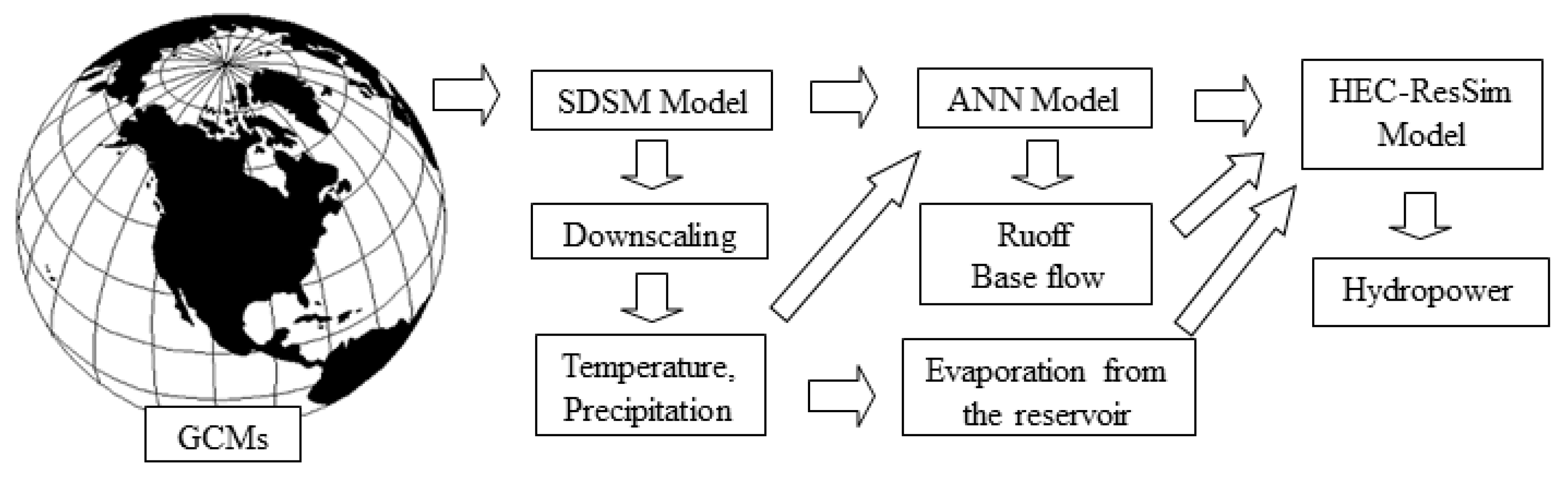
In this study, the performance of the Karun-III dam was evaluated in terms of hydropower production in two future periods according to a combination of the statistical downscaling model (SDSM), artificial neural network (ANN) and HEC-ResSim tools. Figure 1 demonstrates the methodology of the presented study in a schematic way.
2.1. General Circulation Models (GCMs)
The first step involved selection of appropriate general circulation models (GCM) and emission scenarios. In this study, the UK Hadley Center Coupled Model (HadCM3) was selected. This model was developed in 1999 in the Hadley Center of the UK meteorological office and is one of the main models used in the IPCC’s third, fourth and fifth assessment reports. The capability of this model in simulating the current climate without using flux adjustment was a main advantage at the time of its development and this feature still ranks the model highly in comparison to other models [33]. Atmospheric components of the HadCM3 consist of 19 layers with 2.5° × 3.75° (latitude by longitude) horizontal resolution, which produce a global grid of 96 × 73 grid cells with surface spatial resolution of about 417 km × 278 km at the equator, decreasing to 295 km × 278 km at 45° north and south latitude. Oceanic components of this model have 20 layers with 1.25° × 1.25° horizontal resolution that simulate important details of the present oceanic structure [33,34,35].
In this study, HadCM3 output under A2 and B2 emission scenarios was used to evaluate the probable climate change impacts for the two future tri-decadal periods: near (2020–2049) and far (2070–2099). Climatic data includes observed daily precipitation and maximum and minimum temperature at meteorological stations as the predictands, and large-scale meteorological variables as predictors. Among existing downscaling models, a statistical downscaling model (SDSM) is preferred because of its ability to reproduce various statistical characteristics of the observed datasets in its downscaled outputs at a 95% confidence level, which is an advantage over other statistical models such as Lars-WG and ANN [16]. Simulating the local scale daily precipitation and temperature is based on large-scale atmospheric variables including reanalysis datasets (1971–2000) from National Centers for Environmental Prediction (NCEP), and HadCM3 outputs (1971–2099). These large-scale atmospheric variables ensure model consistency in weather generation with adjusting the grid size of HadCM3 outputs to the local scale in the observed period [36,37].
2.2. Statistical Downscaling Model (SDSM)
The SDSM is a hybrid model and multiple regression-based tool for simulating future scenarios to assess the impact of climate change. This model is an integration of a stochastic weather generator approach and a transfer function model and utilizes a linear regression method and a stochastic weather generator [14,21,38,39]. For obtaining the best statistical relationship between the observed and generated climate variables, SDSM provides adjustment during the model calibration in some parameters such as event threshold, bias correction, and variance inflation [21].
SDSM inputs are the datasets of large-scale predictors (NCEP and GCMs) of a grid box close to the study area and local predictands (e.g., temperature, precipitation) at single stations. Regarding the dissimilarity in spatial resolutions of NCEP data (2.5° × 2.5°) and HadCM3 data (2.5° × 3.75°), the NCEP data was interpolated for adjusting its resolution to the same scale as the HadCM3 model [21]. Then all atmospheric data (predictors) were normalized with respect to their 1971–2000 averages and standard deviations [21,40,41].
Finding the most relevant predictor variables by linear correlation analysis between predictors and predictands is critical in SDSM [38]. The most relevant and appropriate combination of predictors has to be chosen by investigating the correlation between the predictand variable and predictor variables (NCEP data), e.g. sea level pressure, temperature, humidity, vorticity and wind direction [14,38,39]. Figure 2 represents the simplified schematic downscaling procedure in SDSM. It is notable that SDSM downscales temperature better than precipitation; however, precipitation time series that are synthesized by the SDSM are acceptable [18,42].
2.3. Runoff Prediction by Artificial Neural Network Model (ANN)
In this study, the ANN model was used because of its common use in the field of hydrology and water resources engineering for predictive purposes and simulating the rainfall–runoff processes [24,43]. Among various ANN architectures, the feed-forward architectures are the most popular and widely used in hydrology and the most common form of them is multilayer perceptrons (MLPs) [24,44]. The computational efficiency of ANNs without using physical components in modelling complex hydrological and water resource behaviors makes it a substitute for conceptual watershed modeling [24,43,45]. Acceptable and satisfactory performance of ANN in the majority of the research in rainfall–runoff modeling makes it an attractive approach to this topic [45].
In feed-forward networks, the information propagation is from an input layer to the output layer. A MLP is a set of neurons that are arranged in different layers: one input layer, one or more hidden layer(s), and one output layer [46,47]. ANN, with one hidden layer, can accurately solve hydrological problems and simulate the nonlinear characteristics of a hydrological process [48].
In this study, a feed-forward MLP ANN model was trained with standard back propagation (BP) against historic monthly runoff of the reservoir. Then, downscaled precipitation and temperature of the future were utilized as the input to the ANN model to estimate the basin runoff. ANN implicitly incorporates the snowmelt contribution in the total stream flow by taking temperature as one of its inputs. In a feed-forward BP-ANN, the nodes of the input layer receive the normalized dataset as inputs [46].
2.4. HEC-ResSim Reservoir Model
The HEC-ResSim 3.0 model is used for simulating reservoirs under various operational rules of water resources allocation, flood control, river routing, and other applications with different operational policies. The user may apply different managements in the reservoir system through defining operational rules and scenarios. Model inputs consist of reservoir properties (volume-area-elevation curve, operational levels, operation rules, etc.), control and operational characteristics, river routing properties, and time series input data. The outputs of this model can be used in water resources planning and management, water supplies allocation, dam reservoirs design, environmental issues, hydroelectric power and flood control planning [49]. In this study, this model was used for hydroelectric power simulation in the Karun III dam.
2.5. Calibration and Validation Assessment
The performance of the model calibration and validation can be evaluated by the following four statistical indices:
where RMSE is the root mean square error, MAE is the mean absolute error, is predicted data, is observed data, is the average of observed data, is the average of predicted data, and n is the number of data.
2.6. Case Study
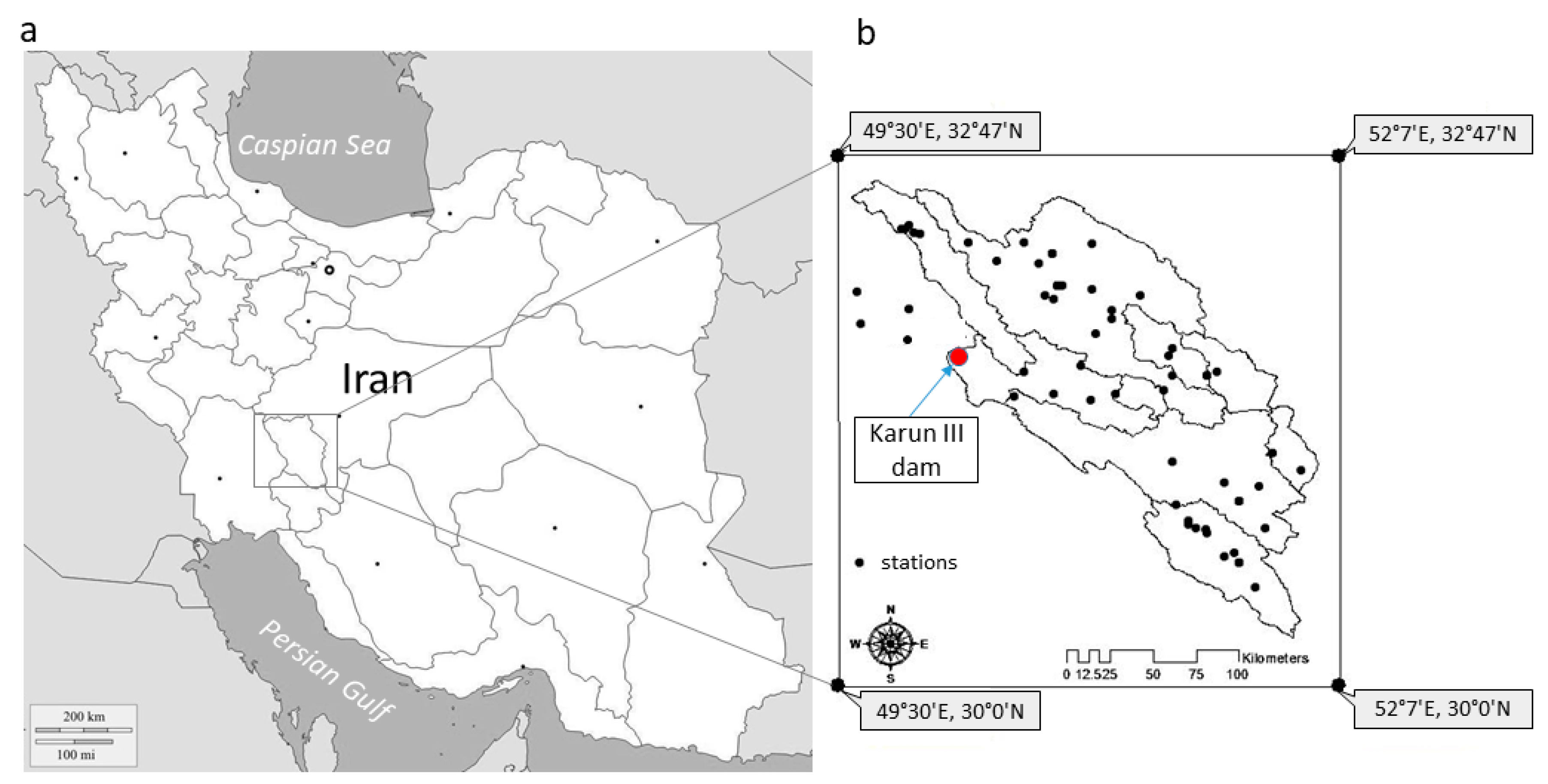
The Karun River basin (Figure 3) is located in southwestern Iran, approximately 28 km from Izeh City and about 610 km from the mouth of the Karun River in north-east Khuzestan Province. This region’s climate is moderate with an annual mean precipitation of 620 mm at the site of the Karun-III dam. The Karun River is the longest river (~950 km) in Iran, extending from the Zagros ridges to the Arvandrud transboundary river junction [50]. The Zargos Mountain Range is considered an exceptional source of hydropower because of considerable precipitation, which provides various river basins with snowmelt and surface runoff, and facilitates powerful streamflow [5]. Annual mean flow of the Karun River at the Karun-III dam site is over 300 m3/s with an annual volume of 106 m3. The reservoir of the Karun-III dam is 60 km long with a surface area of 48 km2 and a storage volume of 2,970,000,000 m3 [50]. The dam was commissioned in 2005 [51]. The Karun III dam is an over-year regulation dam and has been built for hydropower generation as well as to provide more flood control capacity in coordination with other dams built on the Karun River, as well as supplying approximately one billion m3 water for irrigation. The area of the Karun-III dam basin is 24,202 km². The water stored in the Karun-III reservoir is exploited exclusively for hydropower through a hydropower plant with an installed capacity of 2000 MW and 4137 Gwh mean annual energy generation [50,52].
3. Results and Discussion
3.1. Calibration and Validation of SDSM
After evaluating the performance of the SDSM model in downscaling climatic variables, i.e., precipitation and temperature at different meteorological stations over the Karun-III basin, precipitation was downscaled to the basin scale in each station based on the calibrated model. Subsequently, precipitation time series were generated for each rain station. Rainfall is a conditional process and is projected by a stochastic weather generator conditioned on the predictor variables [21]. The precipitation dataset is not generally normalized and because of the skewed nature of the precipitation distribution, the fourth root transformation was applied in this study [21,39]. The observed time series of temperature and precipitation were divided into two periods: the calibration period 1971–1985 for developing the SDSM, and the validation period 1986–2000 for testing the model performance and comparing it with the downscaled results. In the validation period, monthly mean values of precipitation and temperature were downscaled with predictor variables of NCEP reanalysis data.
The monthly average of 20 simulated series of precipitation and maximum and minimum temperature demonstrated a good correlation with the observed precipitation in the calibration period. Table 1 shows the values of statistical measures between observed and downscaled monthly mean precipitation and temperature in the validation period (1986–2000).
3.2. Scenario Projection
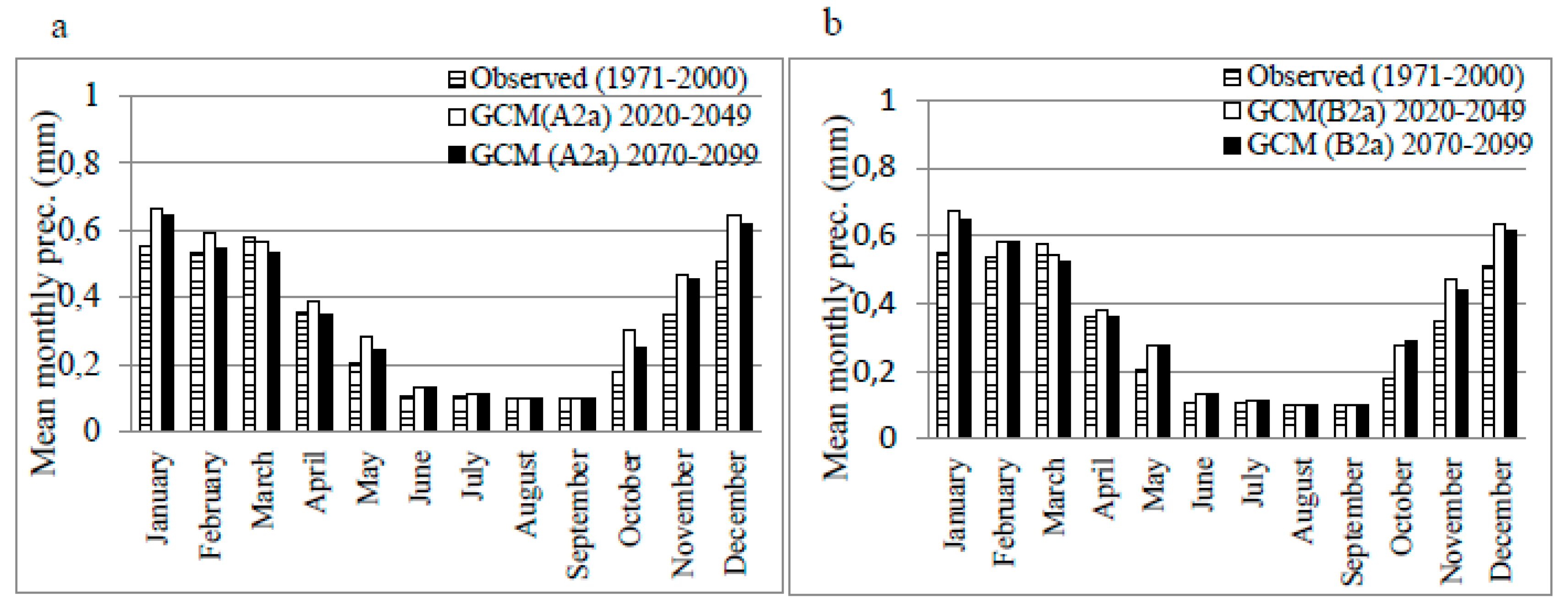
In this section, 20 daily time series of precipitation and maximum and minimum temperature were generated by the predictor variables of the HadCM3 general circulation model under A2 and B2 emission scenarios for the two future tri-decadal periods: near (2020–2049) and far (2070–2099), and then compared with the 1971–2000 control period. The control period in this study as proposed by the World Meteorological Organization (WMO) in climate change studies was the 1971–2000 period after the 1961–1990 baseline [54]. The results are shown in Figure 4.
As clearly seen in Figure 4, the A2 and B2 scenarios have a similar trend in predicting precipitation in the future. Precipitation increases in both scenarios over the near future and far future, except in the month of March. Moreover, the results of the A2 scenario showed a decrease in April over the far future. Changes in summer precipitation were not significant in both periods because of the usual dry summers in this catchment. Furthermore, according to predictions, a larger increase in precipitation is expected in the near future than the far future.
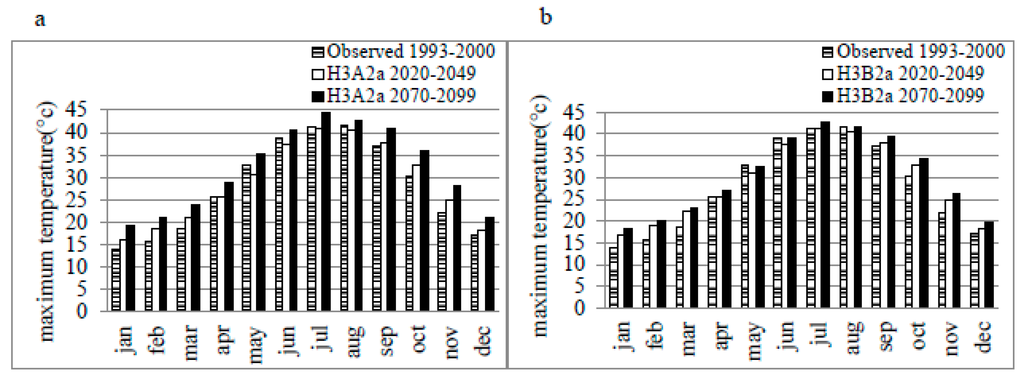
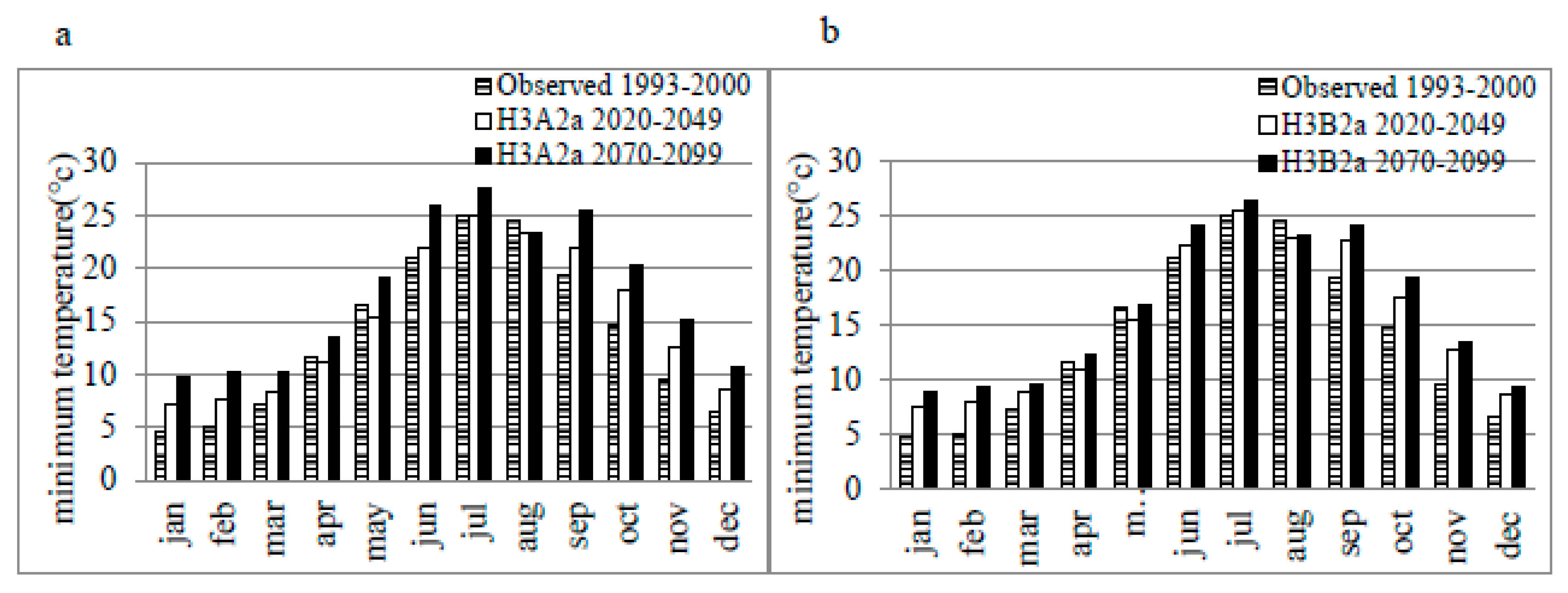
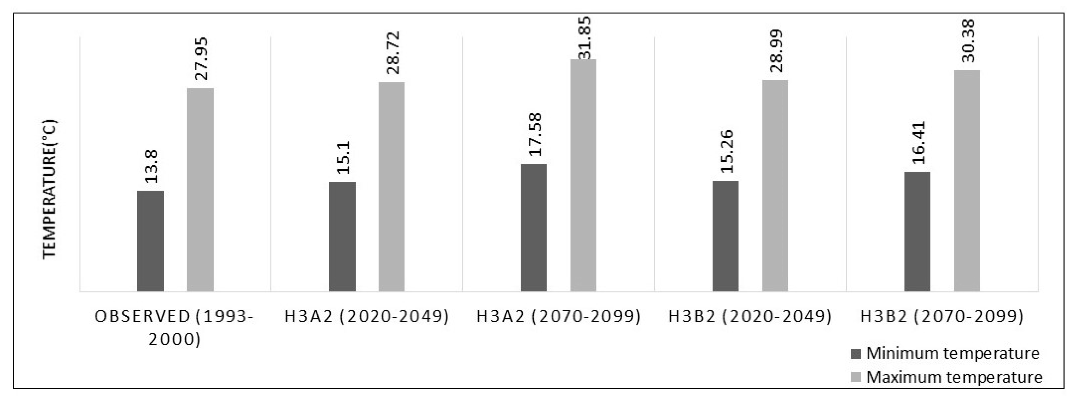
Figure 5 and Figure 6 demonstrate respectively the average monthly observed and predicted maximum and minimum temperatures under A2 and B2 emission scenarios for the two future tri-decadal periods. In addition, Figure 7 presents the average annual temperature changes in the observed and under study periods for both emission scenarios.
As shown in Figure 5, Figure 6 and Figure 7, temperature will increase in both periods under the A2 and B2 scenarios and the Karun-III catchment will become warmer. Compared with the observed period, annual mean maximum and minimum temperatures rise by 1.3 °C and 0.8 °C in 2020–2049 period, and by 3.8 °C and 3.9 °C in the 2070–2099 under the A2 scenario. Similarly under the B2 scenario, the annual average maximum and minimum temperatures increase by 1.5 °C and 1.04 °C in 2020–2049, and by 2.6 °C and 2.4 °C in 2070–2099 over the observed period 1993–2000. The results are compatible with predictions reported in similar researches [42,55].
3.3. Rainfall–Runoff Model
The ANN model was trained with the Levenberg–Marquart (LM) or standard back-propagation (BP) to simulate monthly runoff into the reservoir. The number of neurons in the hidden layer varied between 4 to 7 neurons and was determined through trial and error. Two ANN models were prepared, one for wet and the other for dry seasons, i.e., two 6-month classes including wet months (December–May) and dry months (June–November) out of monthly-observed runoff over the 1971–2000 period. Table 2 shows the performance of the ANN model during the training and test phases for both wet and dry periods. Results indicate better performance in the wet months than in the dry months.
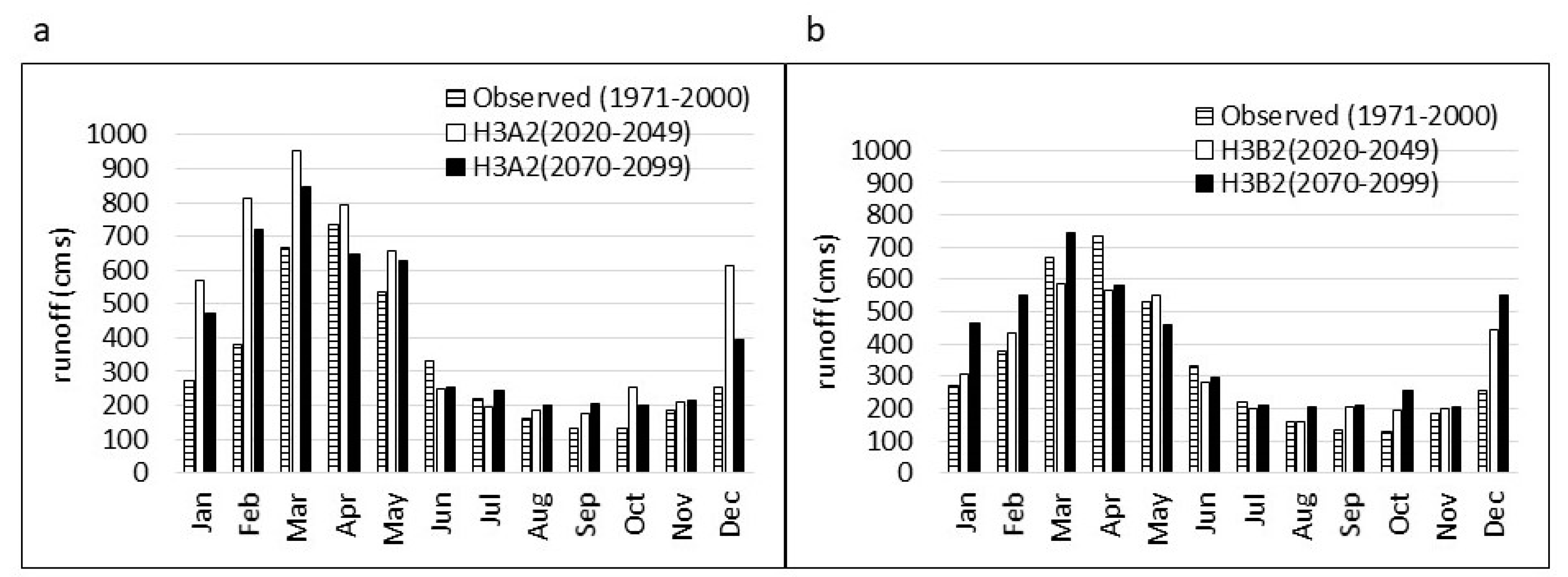
A single ANN model, which encompassed runoff of all months over the year, was also examined. This single ANN model showed better performance than the two separate wet and dry models due to more data for training and testing phases. Therefore, the single ANN model was applied for rainfall–runoff simulation in this study. Figure 8 illustrates the result of the rainfall–runoff simulation by the ANN model for the under study period. Moreover, Table 3 presents the maximum, minimum and average changes in simulated annual runoff in the near and far future compared to the historic period.
The results in Figure 8 showed an increase in runoff of the Karun-III catchment in future periods in comparison with the control period 1971–2000. The stream flow increases more in 2020–2040 than in 2070–2099. Annual average runoff increases by 32.1–51.3% under the A2 scenario and by 17.5–33.7% under the B2 scenario for the near future. The runoff peak also switches from April to March in both scenarios, which is caused by a temperature shift towards a warmer winter to accelerate earlier snowmelt. In contrast, the annual average runoff changes by about −1.5–7.1% under the A2 scenario and 7.5–28.1% under the B2 scenario over the 2070–2099 period.
3.4. Reservoir Evaporation Loss
Evaporation from the surface of the reservoir should be considered for reservoir and hydropower simulations. In this study, the climate change-induced evaporation variation from the surface of the reservoir due to temperature rise in the future was taken into account through an empirical relationship between evaporation and average temperature at a climate station close to the Karun-III dam according to Equation (5):
where T is monthly mean temperature in °C at the climatic station close to the Karun-III dam, and E is the monthly evaporation from the evaporation pan in millimeters.
E = 19.451 T − 144.34
Table 4 demonstrates the statistical indices of the relationship between monthly mean temperature and monthly evaporation in the training and test periods. The evaporation time series for future periods was calculated according to empirical Equation (5).
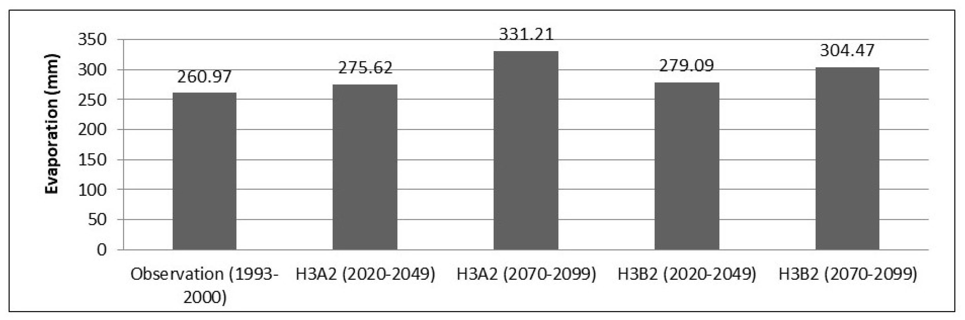
The time series of evaporation for the study period was produced by using Equation (5) and the predicted time series of temperature under A2 and B2 emission scenarios in the near and far future. Figure 9 demonstrates the mean annual evaporation in the observation period and generated time series under A2 and B2 scenarios.
Figure 9 illustrates an increase in evaporation from the surface of the reservoir in the near and far future periods in comparison with the observed period.
3.5. Hydropower Simulation
In this study, the HEC-ResSim reservoir model was used for simulating hydropower in the Karun III dam. Downscaled meteorological variables and evaporation time series were subsequently used as inputs to the HEC-ResSim3.0 reservoir model. To assess the accuracy of the simulation results, the observed time series of hydropower generation in the 2005–2010 period was used for evaluating the model simulation. Table 5 presents the statistical indices of error and correlation of daily hydropower generation between the recorded and simulated time series in the observed period (2005–2010).
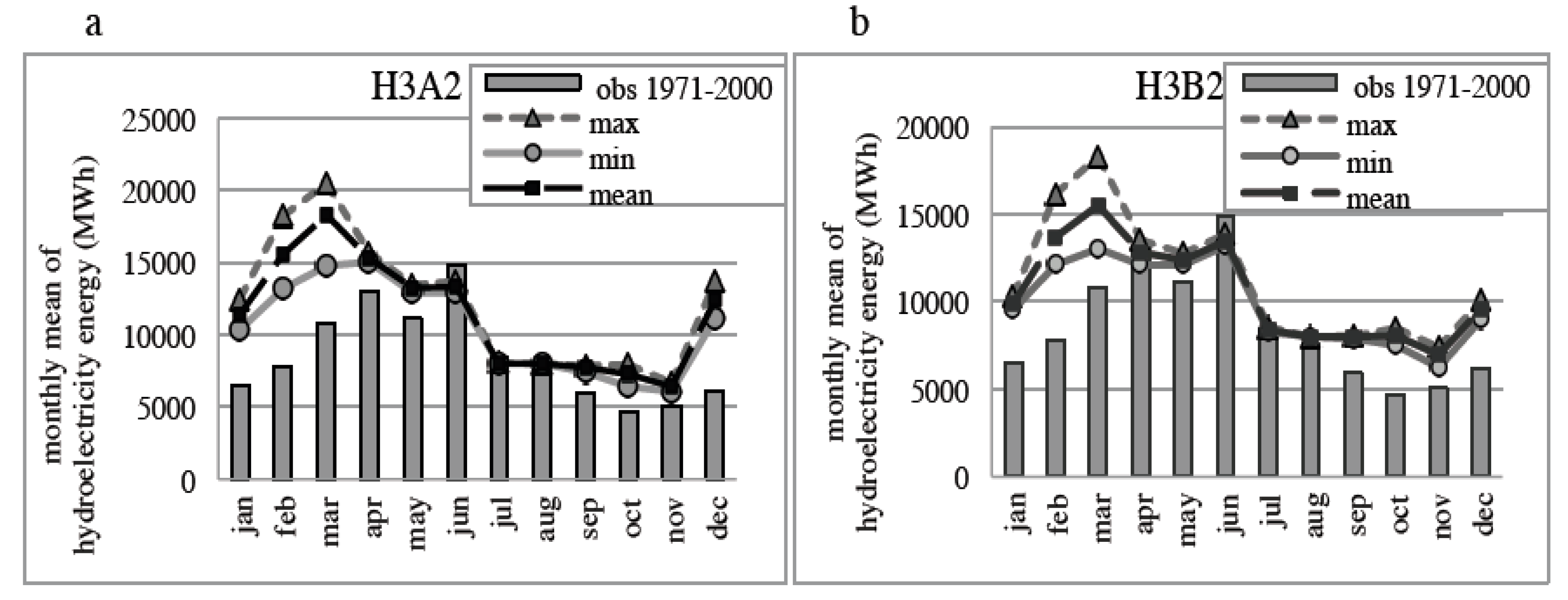
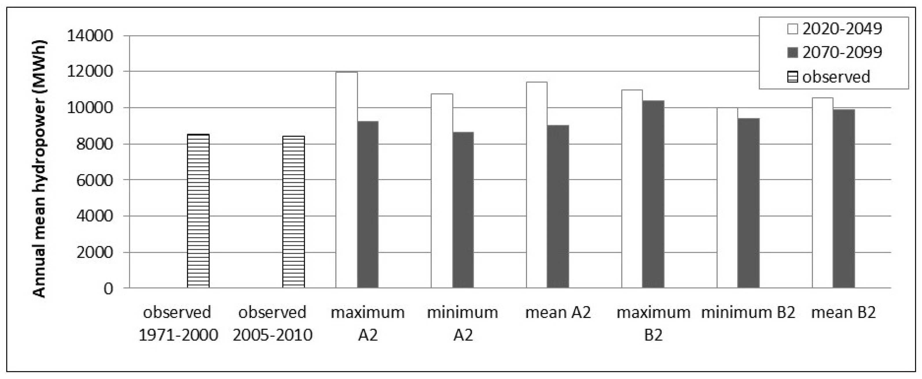
After model calibration, prediction and simulation of hydroelectricity energy for each of the emission scenarios A2 and B2 in the two future periods, as well as for the control period 1971–2000, was conducted. Thus, hydropower energy was simulated according to the observed runoff and surface evaporation data in the control period to serve as the basis of comparison with the future projections. Results of mean, maximum and minimum hydropower generated through 20 monthly runoff series are shown in Figure 10 and Figure 11 for the near and far future, respectively. Furthermore, annual results of different scenarios are presented in Figure 12 and Table 6.
As can be seen in Figure 12 and Table 6, an increase of hydropower generation is expected in future in comparison with the 1971–2000 control period. It is noteworthy that the degree of change in hydropower generation is larger in the near future 2020–2049 than in the far future 2070–2099, which is compatible with the results of simulated runoff data series. Annual average hydropower generation tends to increase gradually by about 26.7–40.5% under A2 and 17.4–29.3% under B2 in the 2020–2049 period. While an increase is simulated in the 2070–2099 period, by about 1.8–8.7% under A2, and 10.5–22% under B2.
While monthly results did not show any overall significant changes in the summer, some changes were predicted in comparison with the control period. Projections under the A2 scenario showed that in the months of June and July of the 2020–2049 period, hydropower energy will be reduced in comparison with the control period. Furthermore, projections under the B2 scenario in the same future period revealed energy reduction in the months of April and June. The hydropower generation peak under both scenarios in the near future shifted to March from June in the control period, which can be justified by the increase in winter precipitation, temperature rise and earlier snowmelt. Additionally, projections in the 2070–2099 period under the A2 scenario exhibited an energy reduction in the months of March, April, June, and July, while the B2 scenario revealed a decrease in the months of April to July. These changes in hydropower production can be due to changes in the stream pattern and rainfall–runoff regime, which are caused by changes in precipitation pattern, temperature rise and abrupt snowmelt. Therefore, it is important to take into consideration climate change impacts on the susceptibility of hydropower generation during the useful life of the dams to mitigate the negative impacts of climate change by sustainable strategic planning and management in the long term.
4. Conclusions
In this study, changes in climatic variables including precipitation, temperature, and evaporation due to climate change over the Karun-III basin in Iran were studied and its impact on hydropower generation in the near (2020–2049) and far (2070–2099) future periods were investigated. The SDSM model was used to simulate the series of precipitation and temperature under climatic scenarios.
Based on the analysis on the downscaled projections of the HadCM3 model under the A2 and B2 scenarios, the Karun-III basin tends to become warmer and wetter by the end of the current century. In all months, except in summer, a precipitation increase will be expected under both scenarios. Projections showed a larger increase in precipitation in the near future than in the far future, while a larger increase in precipitation is expected under the A2 scenario than in the B2 scenario for the 2070–2099 period. It is expected that temperature rise will change the solid atmospheric precipitation (snow and hail) to rain. Therefore, snow reservoirs of the mountains will be reduced.
By simulating the rainfall–runoff process under projected climatic scenarios, it was found that the runoff follows the precipitation pattern. ANN implicitly incorporates the snowmelt contribution in the total runoff by taking temperature as one of the inputs. Annual runoff increased in both the near and far future periods, while stream flow will increase in the near future more than in the far future. The monthly runoff peak also switches from April to March in both A2 and B2 scenarios, which is caused by the increase in winter precipitation, rise in the temperature, earlier snowmelts, dry summers and less snow storage in the mountains.
Evaporation from the surface of the reservoir was also taken into consideration for reservoir and hydropower simulations. The results show an increase in evaporation from the surface of the reservoir in the near and far future periods in comparison with the observed period.
For simulating hydropower generation, downscaled meteorological variables and evaporation time series were subsequently used as inputs to the HEC-ResSim reservoir model. Moreover, hydropower generation under the A2 and B2 climate scenarios were compared with the control period. Results show that annual average hydropower generation tends to increase under A2 and B2 scenarios in both near and far future periods, increasing more in the near future than in the far future.
It is worth mentioning that there are large uncertainties involved in predicting climatic variables as well as simulating future runoff and hydropower under various scenarios. Thus, further studies are required to examine the uncertainty of the results compared to other climate model projections. Moreover, it is important to take into consideration the nexus use of water strategies and need for multipurpose reservoirs. In this study, the irrigation water allocation was assumed to not alter during the study period. This issue should be taken into account in future studies.
In conclusion, mitigation strategies are necessary to offset the negative effects of climate change impacts on hydropower dam planning and operation while trying to capitalize on the positive impacts during certain periods of the future. Although climate change positively impacted hydropower generation in our case study, other aspects must be addressed in other complementary studies for a comprehensive assessment of climate change impacts on various aspects of hydropower dam design and operation in the future.
Author Contributions
M.B. and B.S. conceived and designed the research; A.H. contributed in providing data; M.B. performed the research, analyzed the data and wrote the paper.
Funding
This research received no external funding.
Acknowledgments
Authors would like to express their greatest gratitude to the people who have helped and supported us throughout this study. We are grateful to Sveinung Sægrov, Knut Alfredsen and Ali Tabeshian at NTNU and Yahya Abavi at the University of Southern Queensland for their advice and suggestions. Thanks also to Ameen Razavi and Arezoo Rafiee Nasab for their help and invaluable comments.
Conflicts of Interest
The authors declare no conflict of interest.
References
- Owusu, P.A.; Asumadu-Sarkodie, S. A review of renewable energy sources, sustainability issues and climate change mitig. Cogent Eng. 2016, 3, 1167990. [Google Scholar] [CrossRef]
- Zhang, X.; Li, H.-Y.; Deng, Z.D.; Ringler, C.; Gao, Y.; Hejazi, M.I.; Leung, L.R. Impacts of climate change, policy and Water-Energy-Food nexus on hydropower development. Renew. Energy 2018, 116, 827–834. [Google Scholar] [CrossRef]
- Sternberg, R. Hydropower: Dimensions of social and environmental coexistence. Renew. Sustain. Energy Rev. 2008, 12, 1588–1621. [Google Scholar]
- Ma, Z.F.; Liu, J.; Yang, S.Q. Climate Change in Southwest China during 1961–2010: Impacts and Adaptation. Adv. Clim. Chang. Res. 2013, 4, 223–229. [Google Scholar]
- Blackshear, B.; Crocker, T.; Drucker, E.; Filoon, J.; Knelman, J.; Skiles, M. Hydropower Vulnerability and Climate Change, A Framework for Modeling the Future of Global Hydroelectric Resources; Middlebury College Environmental Studies Senior Seminar: Middlebury, VT, USA, 2011. [Google Scholar]
- IPCC. Summary for Policymakers. In Climate Change 2014, Mitigation of Climate Change; Cambridge University Press: Cambridge, UK, 2014. [Google Scholar]
- IPCC. Summary for Policymakers. In Climate Change 2013: The Physical Science Basis; Cambridge University Press: Cambridge, UK, 2013. [Google Scholar]
- IPCC. Summary for policymakers. Contribution of Working Group II to the Fourth Assessment Report of the Intergovernmental Panel on Climate Change: Impacts, Adaptation and Vulnerability; Cambridge University Press: Cambridge, UK, 2007. [Google Scholar]
- IPCC. Intergovernmental Pannel on Climate Change—IPCC. Climate Change 2007: Synthesis Report; IPCC: Geneva, Switzerland, 2007. [Google Scholar] [CrossRef]
- Randall, D.A.; Wood, R.A.; Bony, S.; Colman, R.; Fichefet, T.; Fyfe, J.; Kattsov, V.; Pitman, A.; Shukla, J.; Srinivasan, J.; et al. Climate Models and Their Evaluation. In Climate Change 2007: The Physical Science Basis. Contribution of Working Group I to the Fourth Assessment Report of the Intergovernmental Panel on Climate Change; Cambridge University Press: Cambridge, UK, 2007. [Google Scholar]
- Chu, J.T.; Xia, J.; Xu, C.Y.; Singh, V.P. Statistical downscaling of daily mean temperature, pan evaporation and precipitation for climate change scenarios in Haihe River, China. Theor. Appl. Clim. 2010, 99, 149–161. [Google Scholar] [CrossRef]
- Liu, W.; Fu, G.; Liu, C.; Song, X.; Ouyang, R. Projection of future rainfall for the North China Plain using two statistical downscaling models and its hydrological implications. Stoch. Environ. Res. Risk Assess. 2013, 27, 1783–1797. [Google Scholar] [CrossRef]
- Sun, Y.; Ding, Y. A projection of future changes in summer precipitation and monsoon in East Asia. Sci. China Ser. D 2010, 53, 284–300. [Google Scholar] [CrossRef]
- Wilby, R.L.; Dawson, C.W.; Barrow, E.M. SDSM—A decision support tool for the assessment of regional climate change impacts. Environ. Model. Softw. 2002, 17, 147–159. [Google Scholar] [CrossRef]
- Fu, G.; Charles, S.P. Statistical downscaling of daily rainfall for southeastern Australia. In Proceedings of the Symposium JH02 Held during IUGG2011, Melbourne, Australia, 28 June–7 July 2011; IAHS Publ 344. IAHS Press: Wallingford, Melbourn, Australia, 2011; pp. 69–74. [Google Scholar]
- Harpham, C.; Wilby, R.L. Multi-site downscaling of heavy daily precipitation occurrence and amounts. J. Hydrol. 2005, 312, 235–255. [Google Scholar] [CrossRef]
- Khan, M.S.; Coulibaly, P.; Dibike, Y. Uncertainty analysis of statistical downscaling methods. J. Hydrol. 2006, 319, 357–382. [Google Scholar] [CrossRef]
- Liu, L.L.; Liu, Z.F.; Xu, Z.X. Trends of climate change for the upper-middle reaches of the Yellow River in the 21st century. Adv. Clim. Chang. Res. 2008, 4, 167–172. [Google Scholar]
- Liu, L.L.; Liu, Z.F.; Xu, Y.; Ren, X.; Fischer, T. Hydrological impacts of climate change in the Yellow River Basin for the 21st century using hydrological model and statistical downscaling model. Quat. Int. 2011, 244, 211–220. [Google Scholar] [CrossRef]
- Arnell, N.W. Climate change and global water resources: SRES emissions and socio-economic scenarios. Glob. Environ. Chang. 2004, 14, 31–52. [Google Scholar] [CrossRef]
- Hassan, Z.; Shamsudin, S.; Harun, S. Application of SDSM and LARS-WG for simulating and downscaling of rainfall and temperature. Theor. Appl. Clim. 2013, 116, 243–257. [Google Scholar] [CrossRef]
- IPCC. Emissions Scenarios. A Special Report of Working Group II of the Intergovernmental Panel on Climate Change; Cambridge University Press: Cambridge, UK, 2000. [Google Scholar]
- Hattermann, F.; Post, J.; Krysanova, V.; Conradt, T.; Wechsung, F. Assessment of water availability in a central-European river basin (Elbe) under climate change. Adv. Clim. Chang. Res. 2008, 4, 42–50. [Google Scholar]
- Maier, H.R.; Jain, A.; Dandy, G.C.; Sudheer, K.P. Methods used for the development of neural networks for the prediction of water resource variables in river systems: Current status and future directions. Environ. Model. Softw. 2010, 25, 891–909. [Google Scholar] [CrossRef]
- Lin, S.-H.; Liu, C.M.; Huang, W.C.; Lin, S.S.; Yen, T.H.; Wang, H.R.; Kuo, J.T.; Lee, Y.C. Developing a yearly warning index to assess the climatic impact on the water resources of Taiwan, a complex-terrain island. J. Hydrol. 2010, 390, 13–22. [Google Scholar] [CrossRef]
- de Jong, P.; Tanajura, C.A.S.; Sánchez, A.S.; Dargaville, R.; Kiperstok, A.; Torres, E.A. Hydroelectric production from Brazil’s São Francisco River could cease due to climate change and inter-annual variability. Sci. Total Environ. 2018, 634, 1540–1553. [Google Scholar] [CrossRef]
- Mishra, S.K.; Hayse, J.; Thomas, V.; Yan, E.; Kayastha, R.B.; LaGory, K.; McDonald, K.; Steiner, N. An integrated assessment approach for estimating the economic impacts of climate change on River systems: An application to hydropower and fisheries in a Himalayan River, Trishuli. Environ. Sci. Policy 2018, 87, 102–111. [Google Scholar] [CrossRef]
- Markoff, M.S.; Cullen, A.C. Impact of climate change on Pacific Northwest hydropower. Clim. Chang. 2008, 87, 451–469. [Google Scholar] [CrossRef]
- Minville, M.; Brissette, F.; Krau, S.; Leconte, R. Adaptation to Climate Change in the Management of a Canadian Water-Resources System Exploited for Hydropower. Water Resour. Manag. 2009, 23, 2965–2986. [Google Scholar] [CrossRef]
- Lehner, B.; Czisch, G.; Vassolo, S. The impact of global change on the hydropower potential of Europe: A model-based analysis. Energy Policy 2005, 33, 839–855. [Google Scholar] [CrossRef]
- Sharma, R.H.; Shakya, N.M. Hydrological changes and its impact on water resources of Bagmati watershed, Nepal. J. Hydrol. 2006, 327, 315–322. [Google Scholar] [CrossRef]
- Harrison, G.; Whittington, H. Vulnerability of Hydropower Projects to Climate Change. IEE Proc. Gener. Transm. Distrib. 2002, 149, 249–255. [Google Scholar] [CrossRef]
- Reichler, T.; Kim, J. How Well Do Coupled Models Simulate Today’s Climate? Bull. Am. Meteorol. Soc. 2008, 89, 303–311. [Google Scholar] [CrossRef]
- Gordon, C.; Cooper, C.; Senior, C.A.; Banks, H.; Gregory, J.M.; Johns, T.C.; Mitchell, J.F.B.; Wood, R.A. The simulation of SST, sea ice extents and ocean heat transports in a version of the Hadley Centre coupled model without flux adjustments. Clim. Dyn. 2000, 16, 147–168. [Google Scholar] [CrossRef]
- Pope, V.D.; Gallani, M.L.; Rowntree, P.R.; Stratton, R.A. The impact of new physical parameterizations in the Hadley Centre climate model—HadAM3. Clim. Dyn. 2000, 16, 123–146. [Google Scholar] [CrossRef]
- Chen, S.-T.; Yu, P.S.; Tang, Y.-H. Statistical downscaling of daily precipitation using support vector machines and multivariate analysis. J. Hydrol. 2010, 385, 13–22. [Google Scholar] [CrossRef]
- Dibike, Y.B.; Coulibaly, P. Hydrologic impact of climate change in the Saguenay watershed: Comparison of downscaling methods and hydrologic model. J. Hydrol. 2005, 307, 145–163. [Google Scholar] [CrossRef]
- He, B.; Takara, K.; Yamashiki, Y.; Kobayashi, K.; Luo, P. Statistical Analysis of Present and Future River Water Temperature in Cold Regions Usings Downscaled GCMs Data; Kyoto University: Kyoto, Japan, 2011; pp. 103–110. [Google Scholar]
- Wilby, R.L.; Dawson, C.W. SDSM 4.2—A Decision Support Tool for the Assessment of Regional Climate Change Impacts. User Manual; Environmental Agency of England and Wales: UK, 2007.
- Samadi, S.; Carbone, G.J.; Mahdavi, M.; Sharifi, F.; Bihamta, M.R. Statistical downscaling of climate data to estimate streamflow in a semi-arid catchment. Hydrol. Earth Syst. Sci. Discuss. 2012, 9, 4869–4918. [Google Scholar] [CrossRef]
- Sarwar, R.; Irwin, S.E.; King, L.M.; Simonovic, S.P. Assessment of Climatic Vulnerability in the Upper Thames River Basin: Downscaling with SDSM; Report No 080; The University of Western Ontario: London, ON, Canade, 2012; ISBN 978-0-7714-2963-7. [Google Scholar]
- Hessami, M.; Gachon, P.; Quarda, T.; St-Hilaire, A. Automated regression-based statistical downscaling tool. Environ. Model. Softw. 2008, 23, 813–834. [Google Scholar] [CrossRef]
- Kasiviswanathan, K.S.; Cibin, R.; Sudheer, K.P.; Chaubey, I. Constructing prediction interval for artificial neural network rainfall runoff models based on ensemble simulations. J. Hydrol. 2013, 499, 275–288. [Google Scholar] [CrossRef]
- Maier, H.R.; Dandy, G.C. Neural networks for the prediction and forecasting of water resources variables: A review of modelling issues and applications. Environ. Model. Softw. 2000, 15, 101–124. [Google Scholar] [CrossRef]
- Bhadra, A.; Bandyopadhyay, A.; Singh, R.; Raghuwanshi, N.S. Rainfall-Runoff Modeling: Comparison of Two Approaches with Different Data Requirements. Water Resour. Manag. 2010, 24, 37–62. [Google Scholar] [CrossRef]
- Agarwal, A.; Mishra, A.K.; Ram, S.; Singh, J.K. Simulation of runoff and sediment yield using Artificial neural networks. Biosyst. Eng. 2006, 94, 596–613. [Google Scholar] [CrossRef]
- Lee, E.; Seong, C.; Kim, H.; Park, S.; Kang, M. Predicting the impacts of climate change on nonpoint source pollutant loads from agricultural small watershed using artificial neural network. J. Environ. Sci. 2010, 22, 840–845. [Google Scholar] [CrossRef]
- Wu, C.L.; Chau, K.W.; Li, Y.S. Methods to improve neural network performance in daily flows prediction. J. Hydrol. 2009, 372, 80–93. [Google Scholar] [CrossRef] [Green Version]
- Klipsch, J.D.; Hurst, M.B. HEC-ResSim Reservoir System Simulation user’s Manual, Version 3.0; US Army Corps of Engineers (USACE): Davis, CA, USA, 2007. [Google Scholar]
- IWPCO. Karun 3 Project; Iran Water & Power Resources Development Co.: Tehran, Iran, 2016. [Google Scholar]
- Mirzabozorg, H.; Hariri-Ardebili, M.A.; Heshmati, M.; Seyed-Kolbadi, S.M. Structural safety evaluation of Karun III Dam and calibration of its finite element model using instrumentation and site observation. J. Case Stud. Struct. Eng. 2014, 1, 6–12. [Google Scholar] [CrossRef] [Green Version]
- Meyer, N.; Ahangari, K. An investigation on stability and support of intake rock slopes of the Karun III dam and power project. In Numerical Modeling of Discrete Materials; Konietzky, H., Ed.; Taylor & Francis Group: London, UK, 2004; pp. 229–234. ISBN 90 58096351. [Google Scholar]
- D-maps.com. 2019. Available online: https://d-maps.com/ (accessed on 30 April 2019).
- IPCC-TGICA. General Guidelines on the Use of Scenario Data for Climate Impact and Adaption Assessment. Version 2; Prepared by Carter, T.R.; on Behalf of the Intergovernmental Panel on Climate Change, Finnish Environment Institute: Helsinki, Finland, 2007. [Google Scholar]
- Abbaspour, K.C.; Faramarzi, M.; Seyed Ghasemi, S.; Yang, H. Assessing the impact of climate change on water resources in Iran. Water Resour. Res. 2009, 45, 1–16. [Google Scholar] [CrossRef]
Figure 1.
Methodology of climate change impact assessment on hydropower generation.

Figure 2.
Diagram of downscaling procedure in statistical downscaling model (SDSM) [38].
Figure 2.
Diagram of downscaling procedure in statistical downscaling model (SDSM) [38].

Figure 3.
Location map of (a) Karun-III watershed in Iran [53], together with (b) the location of the dam and meteorological stations.
Figure 3.
Location map of (a) Karun-III watershed in Iran [53], together with (b) the location of the dam and meteorological stations.

Figure 4.
Values of the average monthly observed and predicted precipitation under (a) A2 and (b) B2 emission scenario in the near and far future.
Figure 4.
Values of the average monthly observed and predicted precipitation under (a) A2 and (b) B2 emission scenario in the near and far future.

Figure 5.
Values of monthly mean observed and predicted maximum temperature under (a) A2 and (b) B2 scenario in the near and far future.
Figure 5.
Values of monthly mean observed and predicted maximum temperature under (a) A2 and (b) B2 scenario in the near and far future.

Figure 6.
Values of monthly mean observed and predicted minimum temperature under (a) A2 and (b) B2 scenario in the near and far future.
Figure 6.
Values of monthly mean observed and predicted minimum temperature under (a) A2 and (b) B2 scenario in the near and far future.

Figure 7.
Comparison between the averages annual observed and downscaled temperature under A2 and B2 scenarios.
Figure 7.
Comparison between the averages annual observed and downscaled temperature under A2 and B2 scenarios.

Figure 8.
Monthly observed and simulated runoff under (a) A2 and (b) B2 scenarios in the near and far future.
Figure 8.
Monthly observed and simulated runoff under (a) A2 and (b) B2 scenarios in the near and far future.

Figure 9.
Mean annual evaporation time series in observation period and A2 and B2 scenarios in the near and far future.
Figure 9.
Mean annual evaporation time series in observation period and A2 and B2 scenarios in the near and far future.

Figure 10.
Range of monthly simulated hydropower energy under (a) A2 and (b) B2 emission scenarios in the 2020–2049 (near future).
Figure 10.
Range of monthly simulated hydropower energy under (a) A2 and (b) B2 emission scenarios in the 2020–2049 (near future).

Figure 11.
Range of monthly simulated hydropower energy under (a) A2 and (b) B2 emission scenarios in the 2070–2099 (far future).
Figure 11.
Range of monthly simulated hydropower energy under (a) A2 and (b) B2 emission scenarios in the 2070–2099 (far future).

Figure 12.
Changes of the annual hydropower in the near and far future under A2 and B2 scenarios compared with the observed periods.
Figure 12.
Changes of the annual hydropower in the near and far future under A2 and B2 scenarios compared with the observed periods.


Table 1.
Values of statistical indices between observed and downscaled monthly mean precipitation and temperature in the validation period (1986–2000).
Table 1.
Values of statistical indices between observed and downscaled monthly mean precipitation and temperature in the validation period (1986–2000).
| Statistical Index | MAE | BIAS | RMSE | Correlation | |
|---|---|---|---|---|---|
| Observed and downscaled precipitation | 13% | 10% | 17% | 97% | |
| Observed and downscaled temperature | Max temperature | 0.26% | 0.04% | 0.33% | 99% |
| Min temperature | 0.83% | 0.03% | 0.96% | 99% | |
Table 2.
Performance criteria of the wet and dry artificial neural network (ANN) model based on precipitation and max and min temperature data.
Table 2.
Performance criteria of the wet and dry artificial neural network (ANN) model based on precipitation and max and min temperature data.
| Train | Test | |||||||
|---|---|---|---|---|---|---|---|---|
| Statistical Index | MAE | BIAS | RMSE | Correlation | MAE | BIAS | RMSE | Correlation |
| Wet (Dec-May) | 29% | 19% | 38% | 87% | 31% | 23% | 38% | 82% |
| Dry (June-Nov) | 26% | 21% | 38% | 75% | 29% | 18% | 39% | 74% |
| All months | 28% | 18% | 38% | 81% | 26% | 17% | 37% | 91% |
Table 3.
Range of predicted changes in annual runoff over the historic period under A2 and B2 scenarios by the end of the century.
Table 3.
Range of predicted changes in annual runoff over the historic period under A2 and B2 scenarios by the end of the century.
| Emission Scenario | A2 | B2 | ||||
|---|---|---|---|---|---|---|
| Changes Compared with Historic Period | Maximum Change | Minimum Change | Average Change | Maximum Change | Minimum Change | Average Change |
| 2020–2049 | +51.3% | +32.1% | +41.7% | +33.7% | +17.5% | +25.6% |
| 2070–2099 | +7.1% | -1.5% | +3.5% | +28.1% | +7.5% | +18.2% |
Table 4.
Statistical indexes of error and correlation of the regression relationship between mean temperature and evaporation.
Table 4.
Statistical indexes of error and correlation of the regression relationship between mean temperature and evaporation.
| Train (1983–1993) | Test (1994–1999) | |||||
|---|---|---|---|---|---|---|
| Statistical Index | RMSE | MAE | Correl | RMSE | MAE | Correl |
| Evaporation | 25% | 19% | 96% | 19% | 15% | 95.7% |
Table 5.
Error indices and correlation coefficient between recorded and simulated hydropower generation in 2005–2010.
Table 5.
Error indices and correlation coefficient between recorded and simulated hydropower generation in 2005–2010.
| Statistical Index: | MAE | BIAS | RMSE | Correlation |
|---|---|---|---|---|
| Daily | 11.8% | 8.4% | 19.6% | 83.3% |
| Monthly | 8.6% | 6.3% | 11.3% | 88% |
Table 6.
Predicted changes of mean annual simulated hydropower energy in the near and far future in comparison with the 1971–2000 period.
Table 6.
Predicted changes of mean annual simulated hydropower energy in the near and far future in comparison with the 1971–2000 period.
| Emission Scenarios | A2 | B2 | ||||
|---|---|---|---|---|---|---|
| Changes in Comparison with Control Period | Maximum Change | Minimum Change | Average Change | Maximum Change | Minimum Change | Average Change |
| 2020–2049 | +40.5% | +26.7% | +34.1% | +29.3% | +17.4% | +24% |
| 2070–2099 | +8.7% | +1.8% | +6.3% | +22% | +10.5% | +16.5% |
© 2019 by the authors. Licensee MDPI, Basel, Switzerland. This article is an open access article distributed under the terms and conditions of the Creative Commons Attribution (CC BY) license (http://creativecommons.org/licenses/by/4.0/).
Share and Cite
MDPI and ACS Style
Beheshti, M.; Heidari, A.; Saghafian, B. Susceptibility of Hydropower Generation to Climate Change: Karun III Dam Case Study. Water 2019, 11, 1025. https://doi.org/10.3390/w11051025
AMA Style
Beheshti M, Heidari A, Saghafian B. Susceptibility of Hydropower Generation to Climate Change: Karun III Dam Case Study. Water. 2019; 11(5):1025. https://doi.org/10.3390/w11051025
Chicago/Turabian StyleBeheshti, Maryam, Ali Heidari, and Bahram Saghafian. 2019. "Susceptibility of Hydropower Generation to Climate Change: Karun III Dam Case Study" Water 11, no. 5: 1025. https://doi.org/10.3390/w11051025
Note that from the first issue of 2016, this journal uses article numbers instead of page numbers. See further details here.