MILP for Optimizing Water Allocation and Reservoir Location: A Case Study for the Machángara River Basin, Ecuador

 , ,
, ,
Abstract
:
1. Introduction
2. Materials and Methods
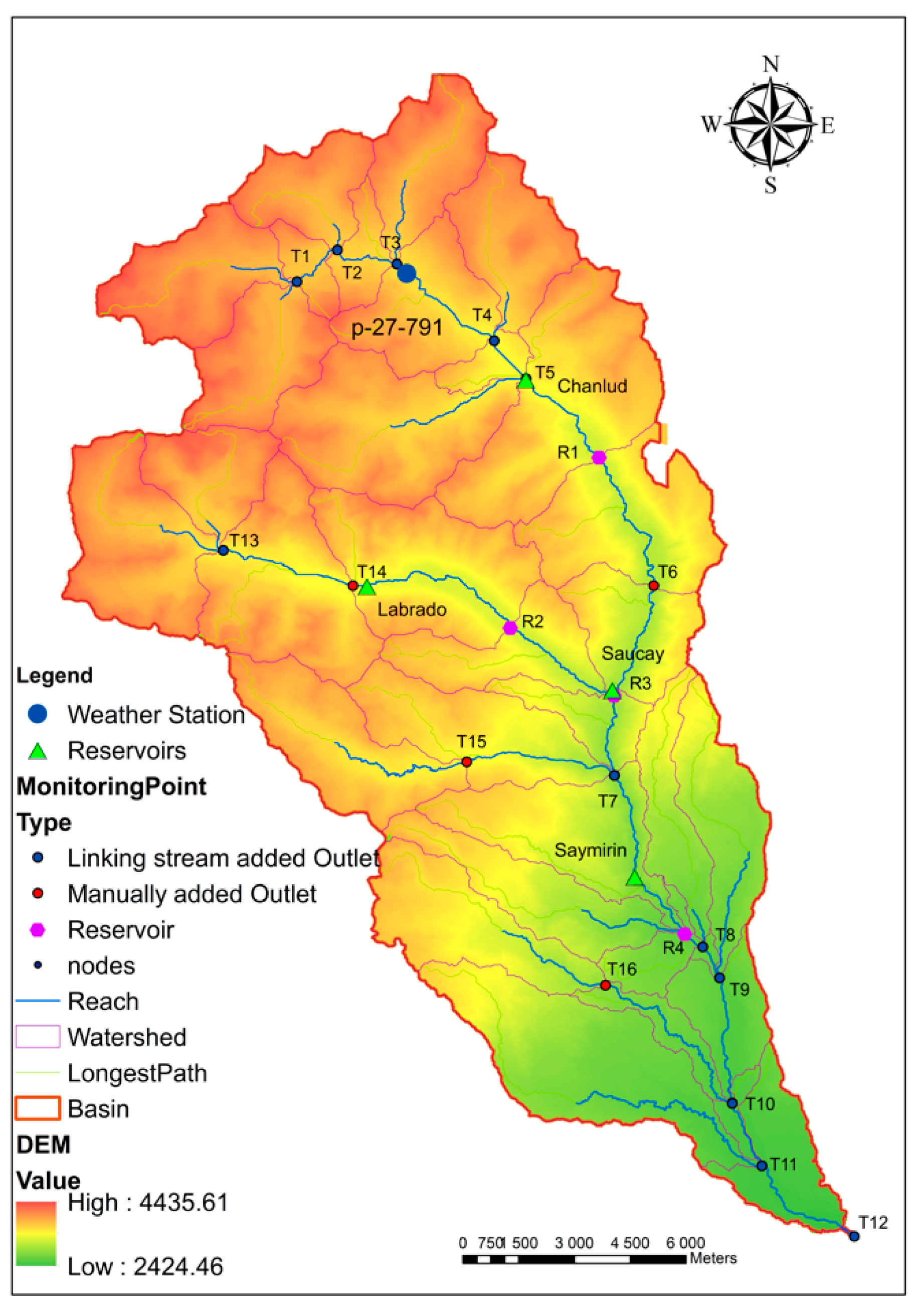
2.1. Study Area
2.1.1. The Machángara River Basin
2.1.2. Reservoirs, Hydropower Production, and Other Water Uses
- The Chanlud Reservoir is located 45 km north of the city of Cuenca. The maximum depth is 51 m and its storage capacity is 17 hm3. The outflow of this reservoir aliments the other two reservoirs (Saucay and Saymirin) as well as the Tixán drinking water treatment plant. This reservoir also aliments several irrigated systems and includes a mechanism to prevent floods [12].
2.2. Linear Programming Model for Optimising Water Allocation
2.2.1. General
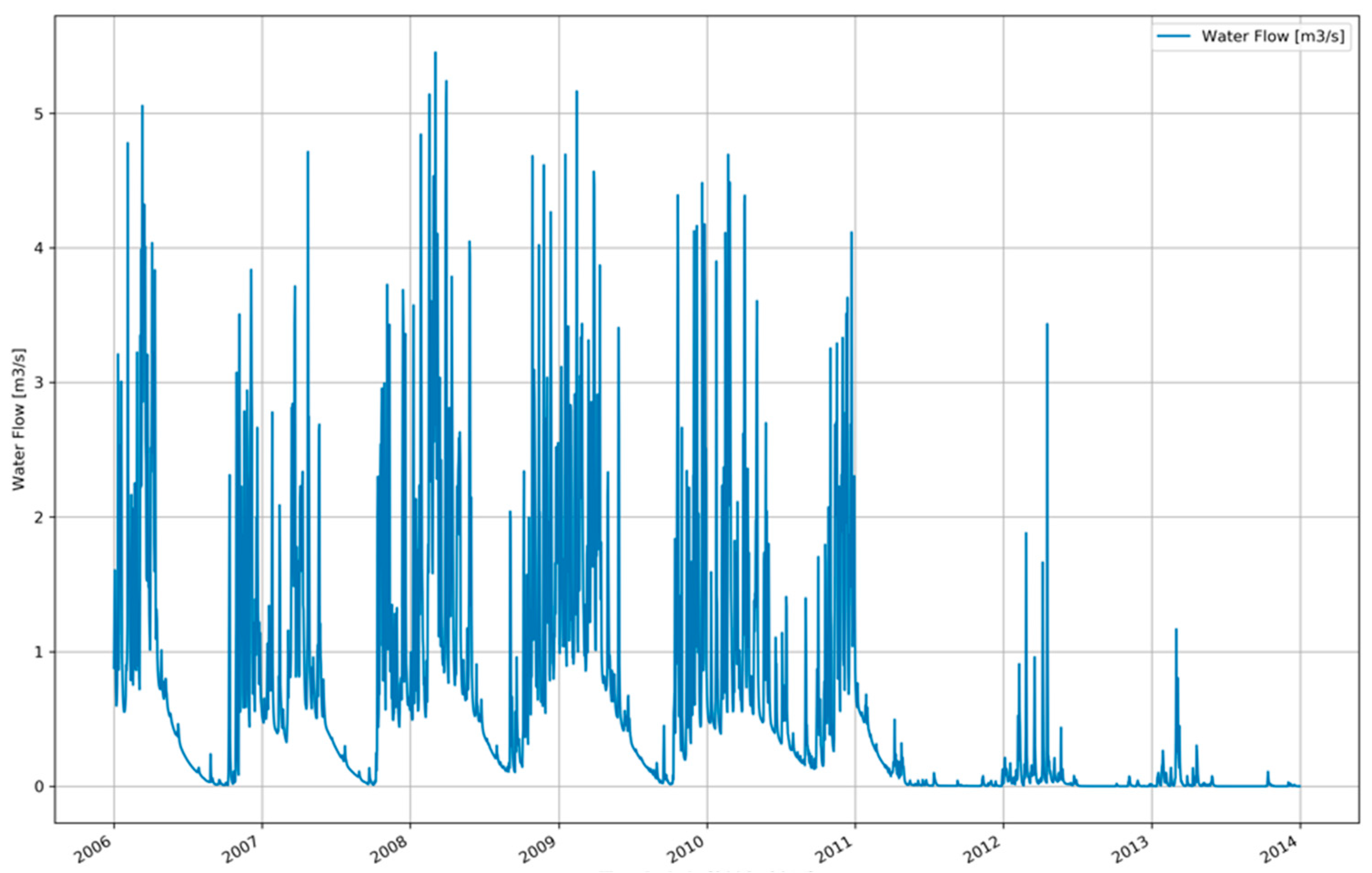
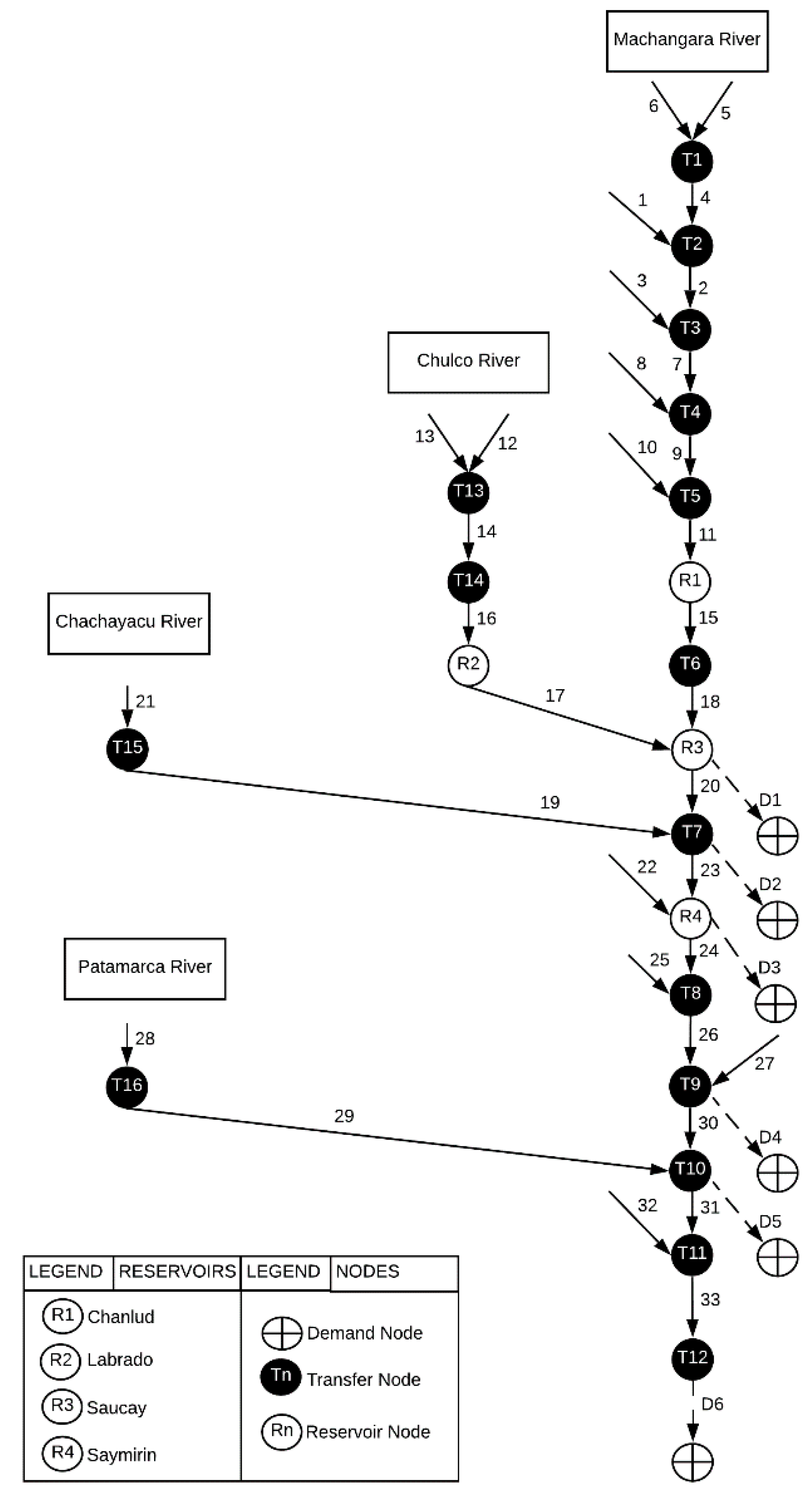
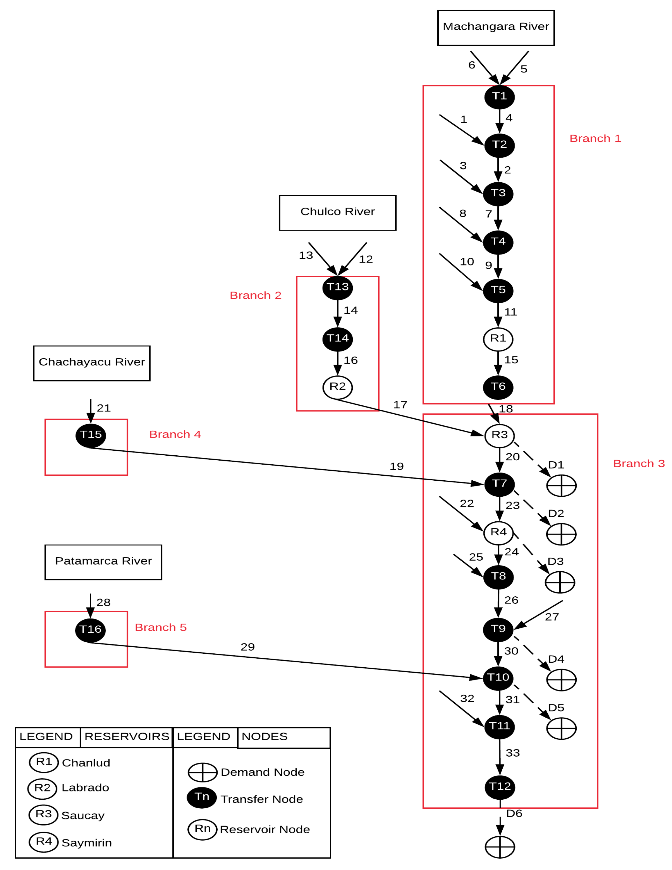
2.2.2. Preliminary River Network Configuration and Water Availability
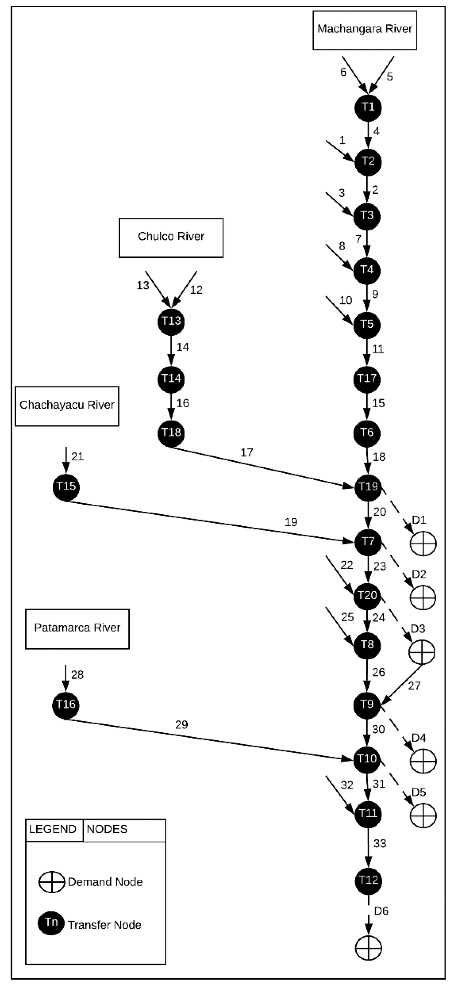
2.2.3. Water Demand and Final River Network Configuration
2.2.4. Objective Function and Constraints
Reservoirs
2.3. Extension of the LP-model into a Mixed Integer Linear Programming Model for Locating Reservoirs
2.3.1. General
2.3.2. Candidate Reservoirs and Capacity
2.3.3. Objective Function and Constraints
Objective Function
Capacity Constraints
3. Results
3.1. Calibration and Validation of LP-Model
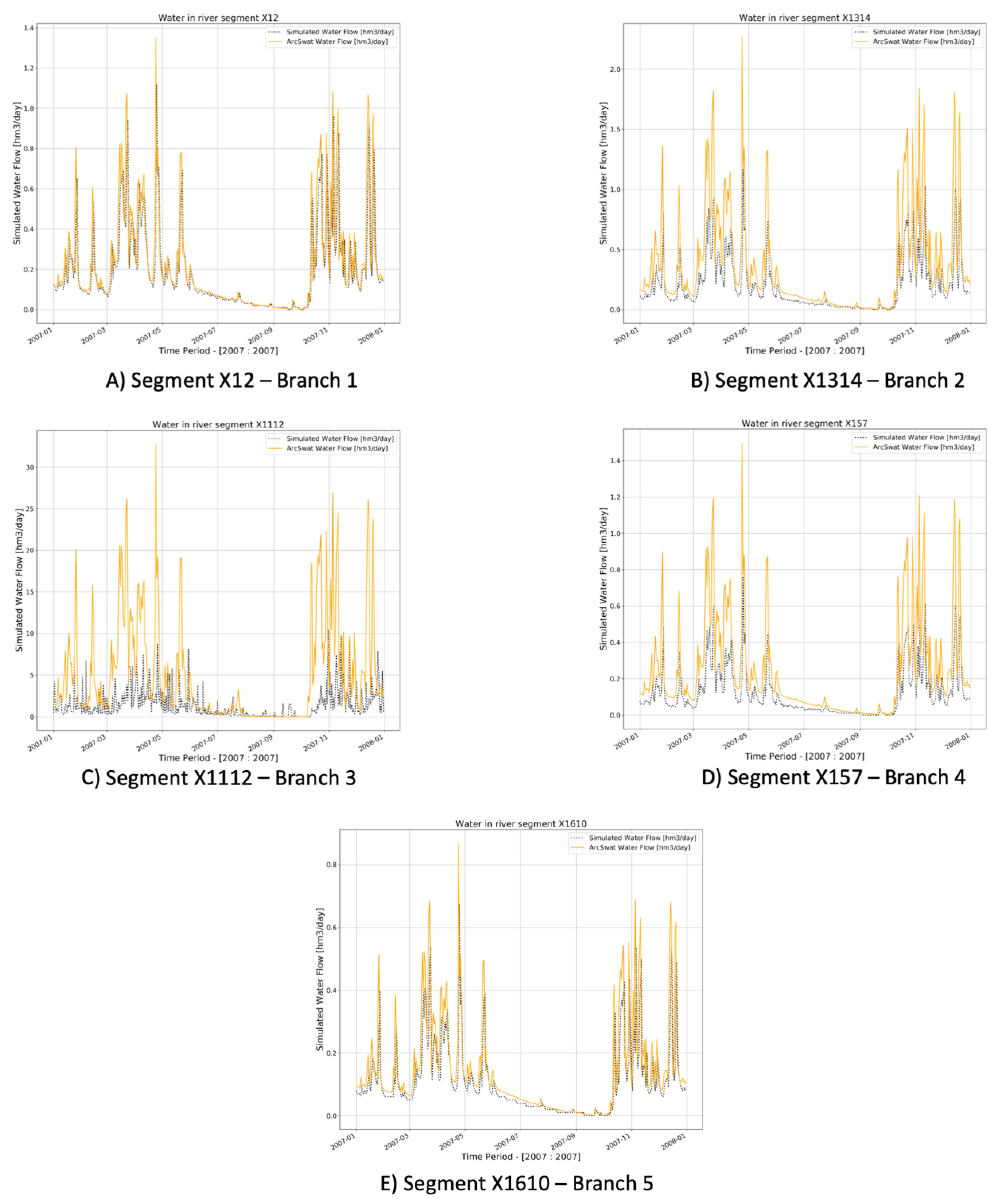
3.1.1. Calibration
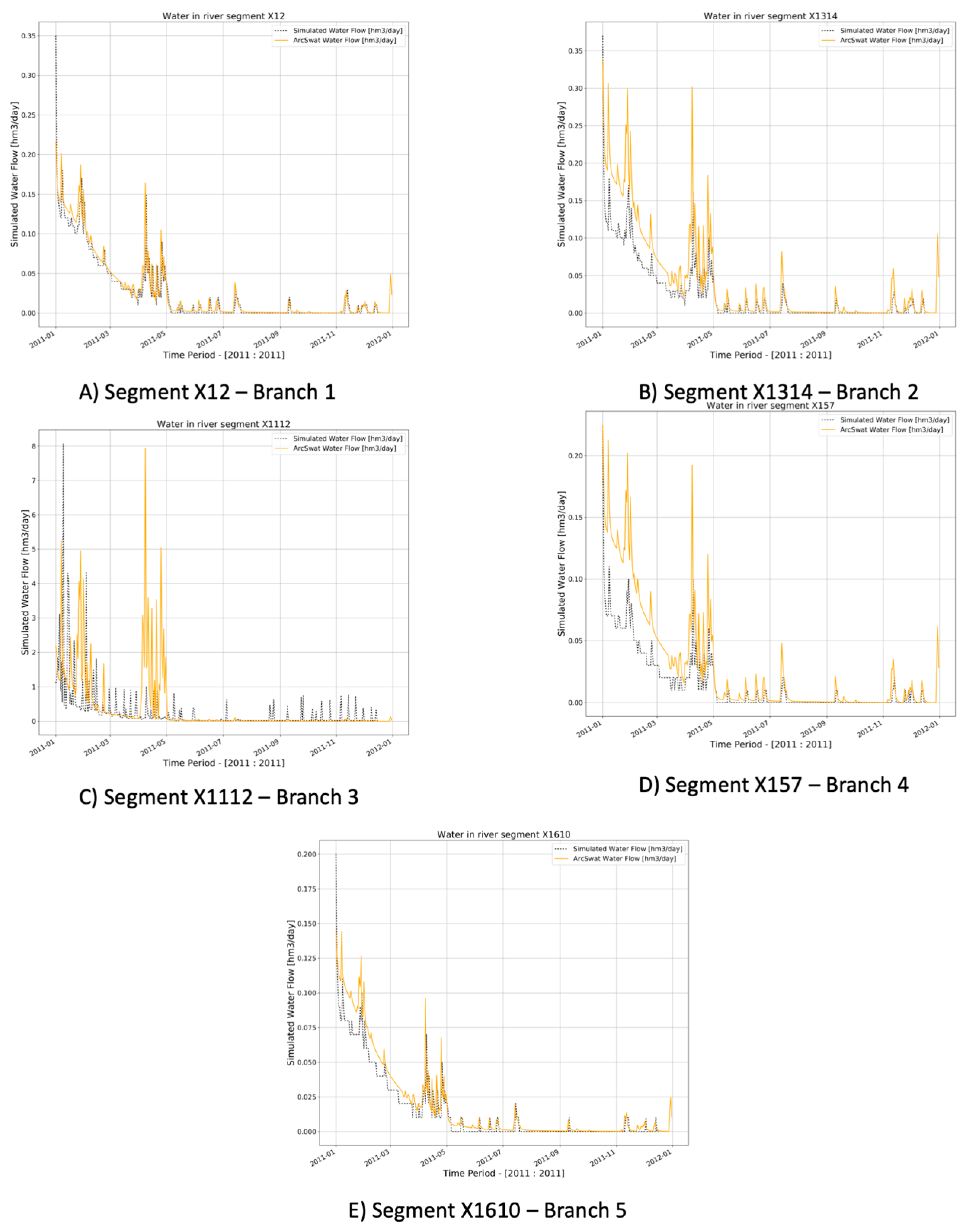
3.1.2. Validation
3.2. Application of the Calibrated and Validated LP-model
3.2.1. Linear Programming Model
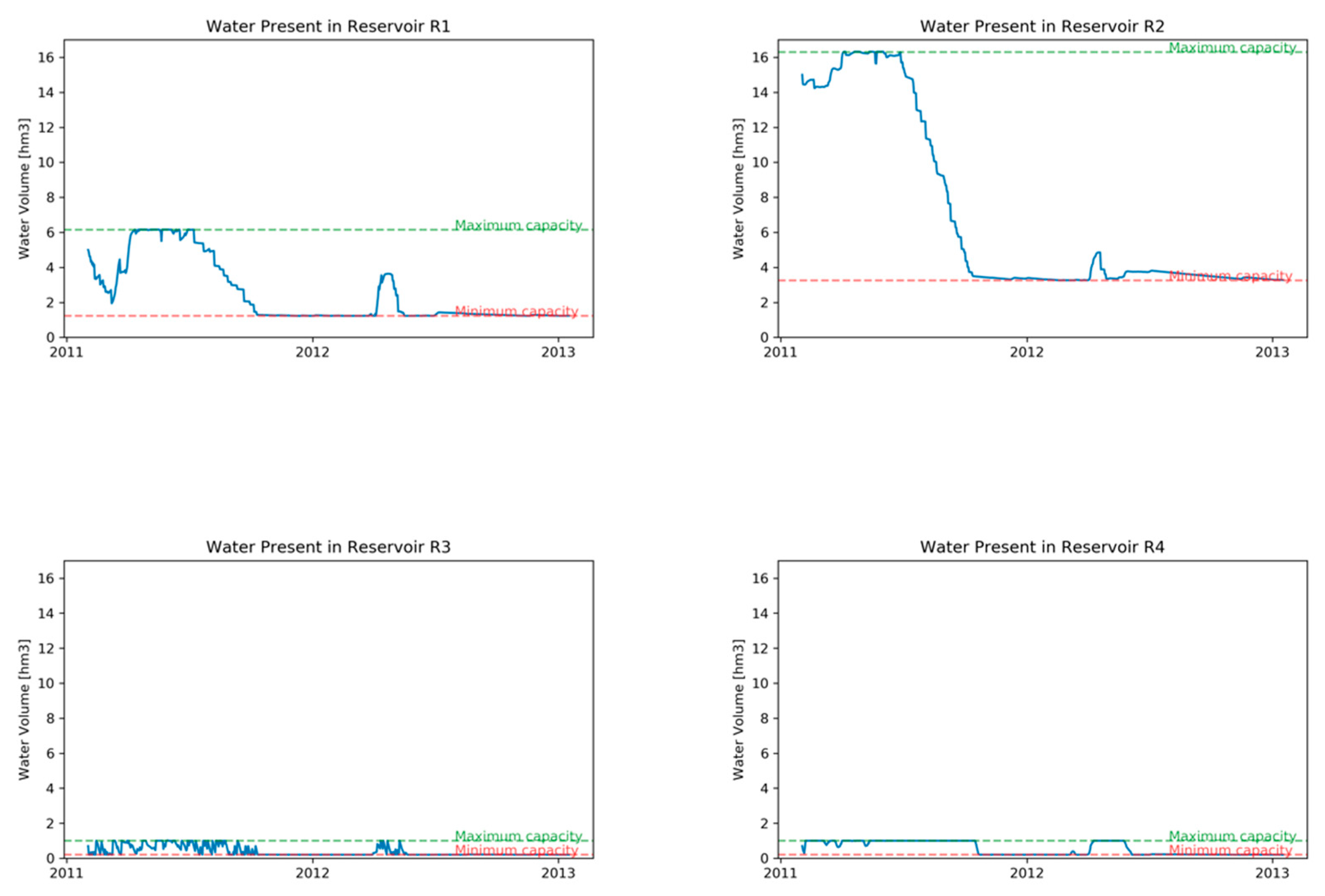
Water in Reservoirs
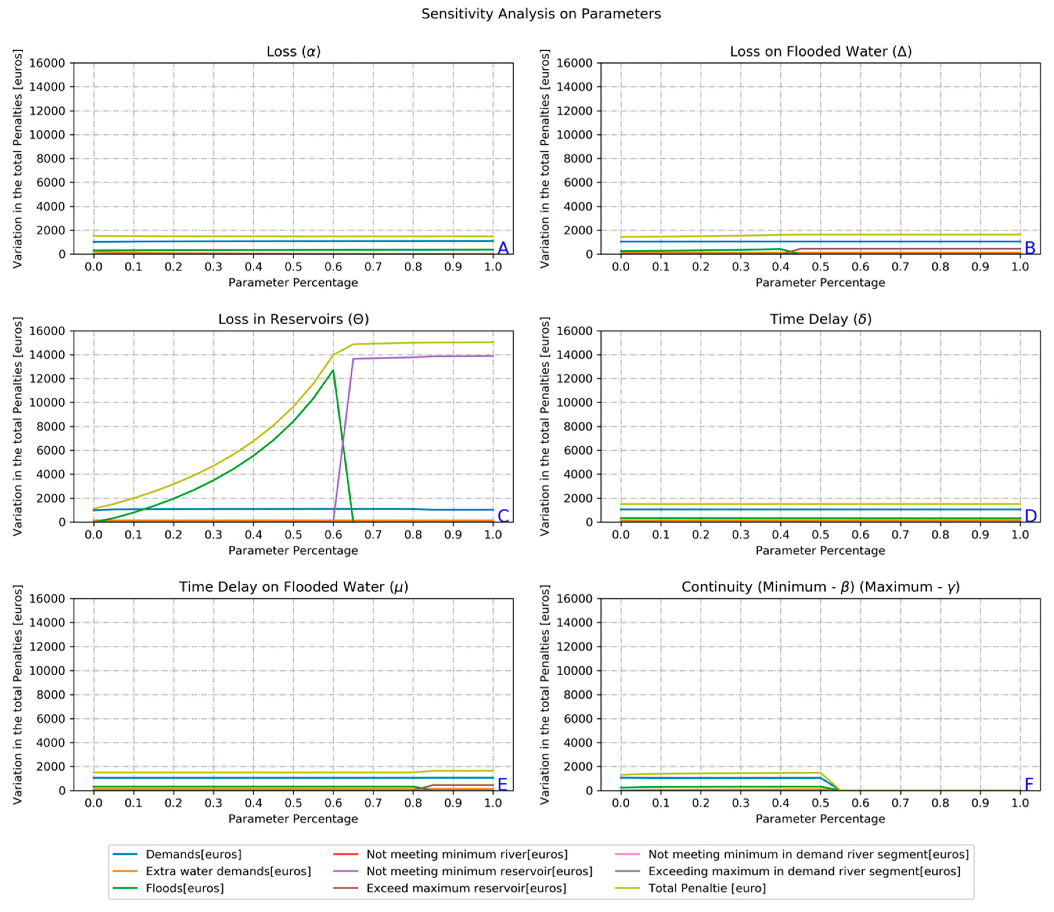
Penalties
3.3. Application of the MILP-Model
Mixed Integer Linear Programming Model
4. Discussion
5. Conclusions
Author Contributions
Funding
Conflicts of Interest
References
- Sharma, B.; Neupane, N.; Amjath-Babu, T.S.; Wahid, S.M.; Sieber, S.; Rasul, G.; Bhattarai, U.; Brouwer, R. Integrated modelling of the impacts of hydropower projects on the water-food-energy nexus in a transboundary Himalayan river basin. Appl. Energy 2019, 239, 494–503. [Google Scholar]
- Liu, P.; Zou, H.; Guo, S.; Zeng, Y.; Shen, Y.; Liu, D.; Zhang, J.; Xiong, L.; Tian, J. Optimisation of water-energy nexus based on its diagram in cascade reservoir system. J. Hydrol. 2018, 569, 347–358. [Google Scholar] [CrossRef]
- Allam, M.M.; Eltahir, E.A.B. Water-Energy-Food Nexus Sustainability in the Upper Blue Nile (UBN) Basin. Front. Environ. Sci. 2019, 7. [Google Scholar] [CrossRef]
- Zeng, X.T.; Zhang, J.L.; Yu, L.; Zhu, J.X.; Li, Z.; Tang, L. A sustainable water-food-energy plan to confront climatic and socioeconomic changes using simulation-optimization approach. Appl. Energy 2019, 236, 743–759. [Google Scholar] [CrossRef]
- Veintimilla-Reyes, J.; De Meyer, A.; Cattrysse, D.; Van Orshoven, J. A linear programming approach to optimise the management of water in dammed river systems for meeting demands and preventing floods. Water Sci. Technol. Water Supply 2018, 18, 713–722. [Google Scholar] [CrossRef]
- Jerves-Cobo, R.; Everaert, G.; Iñiguez-Vela, X.; Córdova-Vela, G.; Díaz-Granda, C.; Cisneros, F.; Nopens, I.; Goethals, P.L.M. A Methodology to Model Environmental Preferences of EPT Taxa in the Machangara River Basin (Ecuador). Water 2017, 9, 195. [Google Scholar] [CrossRef]
- INEC. Resultados del Censo 2010 de Población y Vivienda en el Ecuador. Fascículo Provincial Los Ríos; INEC: Quito, Ecuador, 2010; p. 8. [Google Scholar]
- Jacobsen, D.; Encalada, A. The macroinvertebrate fauna of Ecuadorian highland streams in the wet and dry season. Fundam. Appl. Limnol. 2016, 142, 53–70. [Google Scholar] [CrossRef]
- Texas A&M University. Global Weather Data for SWAT. Available online: https://globalweather.tamu.edu/ (accessed on 6 November 2018).
- Elecaustro. Electro Generadora del Austro—Elecaustro S.A.; Elecautro: Cuenca, Ecuador, 2011. (In Spainish) [Google Scholar]
- Elecaustro. Central Hidroeléctrica Saymirín V Descripción de las Obras de la Central; Elecaustro: Cuenca, Ecuador, 2014. (In Spainish) [Google Scholar]
- Matute, V. Análisis De Factibilidad De Generación Eléctrica A Pie De La Presa De Chanlud. Bachelor’s Thesis, Universidad de Cuenca, Cuenca, Ecuador, 2014. (In Spainish). [Google Scholar]
- Herrera, I.; Carrera, P. Environmental flow assessment in Andean rivers of Ecuador, case study: Chanlud and El Labrado dams in the Machángara River. Ecohydrol. Hydrobiol. 2017, 17, 103–112. [Google Scholar] [CrossRef]
- SENPLADES. Zona de Planificación 6—Austro—Secretaría Nacional de Planificación y Desarrollo. Available online: http://www.planificacion.gob.ec/zona-de-planificacion-6-austro/ (accessed on 31 March 2019). (In Spainish).
- Texas A&M University. ArcSWAT | Soil and Water Assessment Tool. Available online: https://swat.tamu.edu/software/arcswat/ (accessed on 23 July 2018).
- Programa para el Manejo del Agua y el Suelo (PROMAS). Promas. Available online: http://promas.ucuenca.edu.ec/Promas/ (accessed on 6 March 2019). (In Spainish).
- Liu, Q.; Meng, J.; Liu, H.; Chelliah, M.; Ek, M.; Higgins, W.; Xue, Y.; Yang, R.; Keyser, D.; Wang, J.; et al. The NCEP Climate Forecast System Reanalysis. Bull. Am. Meteorol. Soc. 2010, 91, 1015–1058. [Google Scholar]
- Veintimilla-Reyes, J.; De Meyer, A.; Cattrysse, D.; Van Orshoven, J. From Linear Programming Model to Mixed Integer Linear Programming Model for the Simultaneous Optimisation of Water Allocation and Reservoir Location in River Systems. Proceedings 2018, 2, 594. [Google Scholar] [CrossRef]
- Veintimilla-Reyes, J.; Cattrysse, D.; De Meyer, A.; Van Orshoven, J. Mixed Integer Linear Programming (MILP) approach to deal with spatio-temporal water allocation. In Proceedings of the 2nd EWaS International Conference: “Efficient & Sustainable Water Systems Management toward Worth Living Development”, Chania, Crete, Greece, 1–4 July 2016; pp. 1–9. [Google Scholar]
- Veintimilla-Reyes, J.; Cattrysse, D.; De Meyer, A.; Van Orshoven, J. Mixed Integer Linear Programming (MILP) approach to deal with spatio-temporal water allocation. Procedia Eng. 2016, 162, 221–229. [Google Scholar] [CrossRef]
- Google. Google Earth User Guide Getting to Know Google Earth; Google: Parkway Mountain view, CA, USA, 2007; pp. 1–131. [Google Scholar]
- Sultana, Q. Useful Life of a Reservoir and its Dependency on Watershed Activities. Agric. Res. Technol. Open Access J. 2017, 8, 1–9. [Google Scholar] [CrossRef]
- Vaghefi, S.A.; Mousavi, S.J.; Abbaspour, K.C.; Srinivasan, R.; Arnold, J.R. Integration of hydrologic and water allocation models in basin-scale water resources management considering crop pattern and climate change: Karkheh River Basin in Iran. Reg. Environ. Chang. 2013, 15, 475–484. [Google Scholar] [CrossRef]
- Labadie, J.W. MODSIM: Decision Support System for Integrated River Basin Management. Summit Environ. Model. Softw. Int. Environ. Model. Softw. Soc. 2006, 1518–1524. [Google Scholar]
- Shourian, M.; Mousavi, S.J.; Tahershamsi, A. Basin-wide water resources planning by integrating PSO algorithm and MODSIM. Water Resour. Manag. 2008, 22, 1347–1366. [Google Scholar] [CrossRef]
- Pietrucha-Urbanik, K.; Tchorzewska-Cieslak, B. Safety, Reliability and Risk Analysis: Beyond the Horizon; Steenbergen, R., Van Gelder, P., Miraglia, S., Ton Vrouwenvelder, A., Eds.; CRC Press: Boca Raton, FL, USA, 2014; pp. 1115–1120. [Google Scholar]
- Labadie, J.W. Optimal Operation of Multireservoir Systems: State-of-the-Art Review. J. Water Resour. Plan. Manag. 2004, 130, 93–111. [Google Scholar] [CrossRef]
- Hu, Z.; Chen, Y.; Yao, L.; Wei, C.; Li, C. Optimal allocation of regional water resources: From a perspective of equity-efficiency tradeoff. Resour. Conserv. Recycl. 2016, 109, 102–113. [Google Scholar] [CrossRef]
- Devia, G.K.; Ganasri, B.P.; Dwarakish, G.S. A Review on Hydrological Models. Aquat. Procedia 2015, 4, 1001–1007. [Google Scholar] [CrossRef]


| Num. | Demand | Value (hm3 per day) |
|---|---|---|
| D1 | Sucay powerplant | 0.62208 |
| D2 | Machangara irrigation project | 0.0432 |
| D3 | Saymirin powerplant | 0.6912 |
| D4 | Tixan | 0.12096 |
| D5 | “Sociedad riego ricaurte”—irrigation | 0.02592 |
| D6 | Ecosystem | 0.01728 |
| Description | Constraint | |
|---|---|---|
| Objective function | (1) | |
| Flow balance constraints | Transport (n) | |
| (2) | ||
| Reservoir (r) | ||
| (3) | ||
| Network Limitations and capacity constraints | Inputs (i) | |
| (4) | ||
| Sources (i) | ||
| (5) | ||
| Demands (d) | ||
| (6) | ||
| Capacity constraint | River Segments (n) | |
| (7) | ||
| (8) | ||
| Reservoir(r) | ||
| (9) | ||
| (10) | ||
| Demand(d) | ||
| (11) | ||
| (12) | ||
| Continuity constraint | Continuity constraints | |
| (13) | ||
| (14) | ||
| Time Delay | All nodes | |
| (15) | ||
| Flooded Water (n) | ||
| (16) | ||
| Losses | Transfer nodes (n) | |
| (17) | ||
| Reservoir nodes (r) | ||
| (18) | ||
| Demand nodes (d) | ||
| (19) | ||
| Water in Reservoir (r) | ||
| (20) | ||
| Flooded water (n) | ||
| (21) | ||
| Returning water | Returning water to river segments (n) | |
| (22) | ||
| Water returning from a demand | ||
| (23) | ||
| (24) |
| Type | Notation | Description | Unit | Value Use Case |
|---|---|---|---|---|
| Indices | i | input node | - | - |
| r | reservoir node | - | - | |
| d | demand node | - | - | |
| n | transfer node | - | - | |
| t | time step | - | - | |
| Parameters | Penalty for not meeting the demand with one unit | euro/hm3 | 1.0 × 10⁶. | |
| Penalty for exceeding the demand with one unit | euro/hm3 | 2.0 × 10⁷. | ||
| Penalty for not meeting the minimum river segment capacity with one unit | euro/hm3 | 5.0 × 10⁶. | ||
| Penalty for exceeding the maximum capacity in a demand segment with one unit | euro/hm3 | 2.0 ×10⁷. | ||
| Penalty for having a one unit flood in segment (n, n + 1) | euro/hm3 | 4.0 × 10⁶. | ||
| Penalty not meeting the minimum capacity in segment (n, n + 1) with one unit | euro/hm3 | 2.0 × 10⁷. | ||
| Penalty for not meeting the minimum capacity of a reservoir with one unit | euro/hm3 | 8.0 × 10⁶. | ||
| Penalty for exceeding the maximum capacity of a reservoir with one unit | euro/hm3 | 7.0 × 10⁶. | ||
| : | Loss factor associated with the river segment (n, n + 1) at time (t)—to be calibrated | - | 10% | |
| : | Time delay factor associated with the water excess in a river segment (n, n + 1) at time (t) to be calibrated | - | 10% | |
| : | Loss factor associated with the water excess in a river segment (n, n + 1) at time (t) to be calibrated | - | 10% | |
| : | Percentage of water that must flow from the nth node to the next one at time (t), to be calibrated | - | 5% | |
| : | Percentage of water that must remain in the nth node until the next time step (t), to be calibrated | - | 20% | |
| : | Percentage of water that comes to the next node with a time delay in time step (t) to be calibrated | - | 10% | |
| : | Loss factor associated to a reservoir to be calibrated | - | 10% | |
| Minimum capacity of the river segment (n, n + 1) at time (t) | m3 | - | ||
| Maximum capacity of the river segment (n, n + 1) at time (t). The length and width of segment were derived from Google Earth and with a depth of 3m and calculating the cross section [21]. | m3 | - | ||
| Amount of water arriving at the input node (i) at time (t) | m3 | - | ||
| Maximum capacity of a reservoir -> Table 3 | m3 | - | ||
| Minimum capacity of a reservoir -> Table 3 | m3 | - | ||
| Variables | Volume of water in a node (n) at time (t) | m3 | - | |
| Amount of water needed to meet demand (d) in time (t) | m3 | - | ||
| Volume of water in the reservoir (r) at time (t) | m3 | - | ||
| Flow between two nodes, (n) and (n + 1) at time (t) and time (t+1). | m3/day | - | ||
| Flow between a reservoir node (r) and a transfer node (n) at time (t) | m3/day | - | ||
| Flow between a transfer node (n) and a reservoir node (r) at time (t) | m3/day | - | ||
| Flow between an input node (i) and a transfer node (n) at time (t) | m3/day | - | ||
| Flow between an input node (i) and a reservoir node (r) at time (t). | m3/day | - | ||
| Flow between a transfer node (n) and a demand node (d) at time (t) | m3/day | - | ||
| Delayed flow from previous nodes and coming into node (n) at time (t). | m3/day | - | ||
| Water lost during the flow from transfer node (n) to transfer node (n + 1) | m3 | - | ||
| Water lost during the flow from reservoir node (r) to a transfer node (n) | m3 | - | ||
| Water lost during the flow from transfer node (n) to demand node (d) | m3 | - | ||
| Water lost in a reservoir node (r) | m3 | - | ||
| Water lost from the water flooded in the flow process from node (n) to node (n + 1) | m3 | - | ||
| Water delayed from the water flooded in the flow process from node (n) to node (n + 1) | m3 | - | ||
| Water returned from a demand node (d) coming out from a reservoir (r) | m3 | - | ||
| Water delayed from the water flooded in the flow process from node (n) to node (n + 1) | m3 | - | ||
| Slack Variables | Amount of water that cannot be allocated to demand (d) at time (t) | m3 | - | |
| Amount of water above the maximum capacity of node (n) at time (t) | m3 | - | ||
| Amount of water under the maximum capacity of node (n) at time (t) | m3 | - | ||
| Amount of water under the minimum capacity of the node (n) at time (t) | m3 | - | ||
| Amount of water above the minimum capacity of the node (n) at time (t) | m3 | - | ||
| Amount of water above the maximum capacity of the reservoir (r) at time (t) | m3 | - | ||
| Amount of water under the maximum capacity of the reservoir (r) at time (t) | m3 | - | ||
| Amount of water under the minimum capacity of the reservoir (r) at time (t) | m3 | - | ||
| Amount of water above the minimum capacity of the reservoir (r) at time (t) | m3 | - | ||
| Amount of water under the minimum capacity of the demand river segment (d) at time (t) | m3 | - | ||
| Amount of water above the minimum capacity of the demand river segment (d) at time (t) | m3 | - | ||
| Amount of water under the maximum capacity of the demand river segment (d) at time (t) | m3 | - | ||
| Amount of water above the maximum capacity of the demand river segment (d) at time (t) | m3 | - |
| Node | Reservoir | Initial Value (hm3) | Maximum Capacity (hm3) | Minimum Capacity (hm3) | Building + Management Cost (Euros per Two Years) |
|---|---|---|---|---|---|
| 17 | R1 | 5 | 6.15 | 1.23 | 150,000 |
| 18 | R2 | 15 | 16.3 | 3.26 | 215,000 |
| 19 | R3 | 0.7 | 1 | 0.2 | 100,000 |
| 20 | R4 | 0.7 | 1 | 0.2 | 100,000 |
| Branch | Loss Flooded Water (∆) | Time Delay Flooded Water (μ) | |||||
|---|---|---|---|---|---|---|---|
| 1 | 1.0 × 10⁻⁵ | 0.2 | 1.0 × 10⁻⁵ | 0.001 | 0.001 | 0.002 | 0.01 |
| 2 | 1.0 × 10⁻⁵ | 0.2 | 1.0 × 10⁻⁵ | 0.001 | 0.001 | 0.002 | 0.01 |
| 3 | 1.0 × 10⁻⁹ | 0.2 | 1.0 × 10⁻⁹ | 0.001 | 0.001 | 0.002 | 0.01 |
| 4 | 1.0 × 10⁻⁵ | 0.2 | 1.0 × 10⁻⁵ | 0.001 | 0.001 | 0.002 | 0.01 |
| 5 | 1.0 × 10⁻⁵ | 0.2 | 1.0 × 10⁻⁵ | 0.001 | 0.001 | 0.002 | 0.01 |
| Penalties (Euros) | Value (Euros) | Values (Euro/hm3) |
|---|---|---|
| (a) Penalty for not meeting the demands | 920.81 | 920.81 |
| (b) Penalty for exceeding the demands | 3.44 × 10⁸ | 17.17 |
| (c) Penalty flooding of river segments | 0.00 | 0.00 |
| (d) Penalty for not meeting the minimum capacity in the river segments | 0.00 | 0.00 |
| (e) Penalty for exceeding the maximum capacity in reservoirs | 1.82 × 10⁵ | 0.03 |
| (f) Penalty for not reaching the minimum capacity in reservoirs | 0.00 | 0.00 |
| (g) Penalty for not reaching the minimum capacity in demand segments | 0.00 | 0.00 |
| (h) Penalty for exceeding the maximum capacity in demand segments | 0.00 | 0.00 |
| (i) Building + management cost | 5.65 × 10⁵ | 0.00 |
| Total (a) + (b) + (c) + (d) + (e) + (f) + (g) + (h) + (i) | 3.45 × 10⁸ | 938.01 |
| Use Case | Number of Reservoirs | Reservoirs Included in the Solution | Water Not Allocated | Penalties (Euros) | Building + Management (Euros) | Total | |
|---|---|---|---|---|---|---|---|
| 1 | 0 | - | 934.975 | 1.97 × 10⁸ | 0.00 | 1.97 × 10⁸ | |
| 2 | 1 | 12 | 926.707 | 9.27 × 10⁸ | 1.95 × 10⁵ | 9.27 × 10⁸ | |
| 3 | 2 | 12,20 | 926.39 | 9.26 × 10⁸ | 2.95 × 10⁵ | 9.27 × 10⁸ | |
| 4 | 3 | 12,19,20 | 925.429 | 9.25 × 10⁸ | 3.95 × 10⁵ | 9.26 × 10⁸ | |
| 5 | 4 | 11,13,19,20 | 925.094 | 9.25 × 10⁸ | 5.90 × 10⁵ | 9.26 × 10⁸ | |
| 6 | 5 | 10,12,17,19,20 | 916.215 | 9.16 × 10⁸ | 7.40 × 10⁵ | 9.17 × 10⁸ | |
| 7 | 6 | 9,10,12,17,19,20 | 911.807 | 9.12 × 10⁸ | 9.35 × 10⁵ | 9.13 × 10⁸ | |
| 8 | 7 | 9,10,12,13,17,19,20 | 911.329 | 9.11 × 10⁸ | 1.13 × 10⁶ | 9.12 × 10⁸ | |
| 9 | 8 | 9,10,12,13,14,17,19,20 | 910.859 | 9.11 × 10⁸ | 1.33 × 10⁶ | 9.12 × 10⁸ | |
| 10 | 9 | 9,10,12,13,14,15,17,19,20 | 910.315 | 9.10 × 10⁸ | 1.52 × 10⁶ | 9.12 × 10⁸ | |
| 11 | 10 | 8,9,10,12,13,14,15,17,19,20 | 908.859 | 9.09 × 10⁸ | 1.72 × 10⁶ | 9.11 × 10⁸ | |
| 12 | 11 | 7,8,9,10,12,13,14,15,17,19,20 | 908.438 | 9.08 × 10⁸ | 1.91 × 10⁶ | 9.10 × 10⁸ | |
| 13 | 12 | 7,8,9,10,12,13,14,15,16,17,19,20 | 908.38 | 9.08 × 10⁸ | 2.11 × 10⁶ | 9.10 × 10⁸ | |
| 14 | 13 | 7,8,9,10,11,12,13,14,15,16,17,19,20 | 908.324 | 9.08 × 10⁸ | 2.30 × 10⁶ | 9.11 × 10⁸ | |
| 15 | 14 | 6,7,8,9,10,11,12,13,14,15,16,17,19,20 | 907.759 | 9.08 × 10⁸ | 2.50 × 10⁶ | 9.10 × 10⁸ | |
| 16 | 15 | 5,6,7,8,9,10,11,12,13,14,15,16,17,19,20 | 907.267 | 9.07 × 10⁸ | 2.69 × 10⁶ | 9.10 × 10⁸ | |
| 17 | 16 | 4,5,6,7,8,9,10,11,12,13,14,15,16,17,19,20 | 906.703 | 9.07 × 10⁸ | 2.89 × 10⁶ | 9.10 × 10⁸ | |
| 18 | 17 | 3,4,5,6,7,8,9,10,11,12,13,14,15,16,17,19,20 | 906.212 | 9.06 × 10⁸ | 3.08 × 10⁶ | 9.09 × 10⁸ | |
| 19 | 18 | 2,3,4,5,6,7,8,9,10,11,12,13,14,15,16,17,19,20 | 905.701 | 9.06 × 10⁸ | 3.28 × 10⁶ | 9.09 × 10⁸ | |
| 20 | 19 | 1,2,3,4,5,6,7,8,9,10,11,12,13,14,15,16,17,19,20 | 905.166 | 9.05 × 10⁸ | 3.47 × 10⁶ | 9.09 × 10⁸ | |
| 21 | 20 | 1,2,3,4,5,6,7,8,9,10,11,12,13,14,15,16,17,18,19,20 | 872.398 | 8.72 × 10⁸ | 3.69 × 10⁶ | 8.76 x10⁸ | |
© 2019 by the authors. Licensee MDPI, Basel, Switzerland. This article is an open access article distributed under the terms and conditions of the Creative Commons Attribution (CC BY) license (http://creativecommons.org/licenses/by/4.0/).
Share and Cite
Veintimilla-Reyes, J.; De Meyer, A.; Cattrysse, D.; Tacuri, E.; Vanegas, P.; Cisneros, F.; Van Orshoven, J. MILP for Optimizing Water Allocation and Reservoir Location: A Case Study for the Machángara River Basin, Ecuador. Water 2019, 11, 1011. https://doi.org/10.3390/w11051011
Veintimilla-Reyes J, De Meyer A, Cattrysse D, Tacuri E, Vanegas P, Cisneros F, Van Orshoven J. MILP for Optimizing Water Allocation and Reservoir Location: A Case Study for the Machángara River Basin, Ecuador. Water. 2019; 11(5):1011. https://doi.org/10.3390/w11051011
Chicago/Turabian StyleVeintimilla-Reyes, Jaime, Annelies De Meyer, Dirk Cattrysse, Eduardo Tacuri, Pablo Vanegas, Felipe Cisneros, and Jos Van Orshoven. 2019. "MILP for Optimizing Water Allocation and Reservoir Location: A Case Study for the Machángara River Basin, Ecuador" Water 11, no. 5: 1011. https://doi.org/10.3390/w11051011