Modelling Soil Water Dynamics from Soil Hydraulic Parameters Estimated by an Alternative Method in a Tropical Experimental Basin

Abstract

Knowledge about soil moisture dynamics and their relation with rainfall, evapotranspiration, and soil physical properties is fundamental for understanding the hydrological processes in a region. Given the difficulties of measurement and the scarcity of surface soil moisture data in some places such as Northeast Brazil, modelling has become a robust tool to overcome such limitations. This study investigated the dynamics of soil water content in two plots in the Gameleira Experimental River Basin, Northeast Brazil. For this, Time Domain Reflectometry (TDR) probes and Hydrus-1D for modelling one-dimensional flow were used in two stages: with hydraulic parameters estimated with the Beerkan Estimation of Soil Transfer Parameters (BEST) method and optimized by inverse modelling. The results showed that the soil water content in the plots is strongly influenced by rainfall, with the greatest variability in the dry–wet–dry transition periods. The modelling results were considered satisfactory with the data estimated by the BEST method (Root Mean Square Errors, RMSE = 0.023 and 0.022 and coefficients of determination, R² = 0.72 and 0.81) and after the optimization (RMSE = 0.012 and 0.020 and R² = 0.83 and 0.72). The performance analysis of the simulations provided strong indications of the efficiency of parameters estimated by BEST to predict the soil moisture variability in the studied river basin without the need for calibration or complex numerical approaches.

1. Introduction

Surface soil moisture plays a key role in the hydrological cycle as it controls the water fluxes between soil, vegetation, and atmosphere [1,2,3]. Moreover, knowledge about soil moisture is widely required in many agricultural studies and applications related to irrigation management [1,4,5,6]. Therefore, monitoring and understanding of soil moisture variability and its exchange relationships with the surface and atmosphere are essential to improve weather forecasting, flooding and drought predictions, and climate projections [7,8]. However, soil moisture is highly variable in space and time due to the combined influence of many factors in a nonlinear fashion such as the hydraulic properties of the soil, topographic characteristics, interaction with surface water systems, precipitation features, and additional meteorological conditions [3,9,10]. Because of its high variability in natural conditions, achieving accuracy in soil moisture estimation to obtain areal information at different spatial and temporal scales is still a challenging task, especially at high spatiotemporal scales [6,11]. In the last 40 years, the scientific community has clearly recognized the importance of soil moisture as input for earth science applications, developing new approaches and techniques for monitoring, modelling, and use of soil moisture data [12].

Currently, three main approaches are used to provide soil moisture estimates: in situ (generally point-scale) measurements, remote sensing observations, and hydrological modelling applications [12,13]. The most accurate and direct methods to determine soil moisture are related to experimental techniques using classical devices such as soil sampling and Time Domain Reflectometry (TDR) probes [14]. However, these measurements are expensive and time-consuming and provide point-scale information but are unable to detect the spatial heterogeneity of the soil moisture at wider scales [6]. The use of remote sensing and modelling techniques has become a viable solution to overcome the limitations of in situ data [15,16]. For instance, remote sensing techniques provide surface soil moisture estimates over large areas by using active sensors operating in microwave bands that are not influenced by solar radiation and cloud cover [6]. However, the spatial and temporal resolutions of the current remote sensing products are still insufficient for small-scale applications (<1 km²) [17], with soil moisture data only available for the first few centimetres of the soil layer [14,18]. Consequently, they do not cover the soil water in the root zone or over the whole profile, which is most interesting for hydrologists [13]. The limitations imposed by the complex interactions between vegetation, soil, and climate make the use of models based on physical processes an effective and viable (low-cost) alternative for evaluating the spatiotemporal soil moisture trends at different depths [2,19,20].

Many models with different levels of complexity and accuracy have been proposed to simulate the dynamics of water in the unsaturated zone of soil; they include, among others, the Soil Water Atmosphere Plant (SWAP) [21], Soil-Vegetation-Atmosphere Transfer (SVAT) [22], Soil Water Infiltration and Movement (SWIM) [23], Groundwater Loading Effects of Agricultural Management Systems (GLEAMS) [24], Water and Agrochemicals in the soil, crop and Vadose Environment (WAVE) [25], and Hydrus models. Most of the abovementioned models use the Richards’ equation to represent the movement of water in unsaturated soil [26], allowing a detailed description of the soil water content distribution and fluxes inside the soil domain [27]. Hydrus-1D model is one of the most common numerical solutions based on the Richards’ equation [28]. Over the years, Hydrus-1D model has been successfully applied in various studies worldwide for predicting soil moisture content and water movement under different conditions (e.g., [13,29,30,31,32,33]). As a physically based model, Hydrus-1D requires some input data for simulations such as meteorological data for surface boundary conditions, soil physical conditions, and physical parameters (saturated hydraulic conductivity and soil water retention curve), which may be obtained through experimentation [27,34,35,36]. Moreover, according to Bordoni et al. [2], for a better implementation of this type of model, a preliminary calibration of some hydrological parameters used in the methodology is sometimes required.

When performed in the laboratory, the methods commonly used to determine soil physical parameters may not be accurate enough to represent the actual field conditions or may be tedious and time-consuming [36,37]. As an alternative, the scientific community has developed simplified methods that are very often able to provide more accurate results, such as Beerkan [38,39]. Beerkan is a simple and easy method based on in situ single-ring water infiltration experiments which can be carried out in the field at low cost [40]. BEST (Beerkan Estimation of Soil Transfer Parameters) is an algorithm presented by Lassabatere et al. [41] which makes it possible to process the infiltration tests carried out using the Beerkan method [42]. The Hydrus-1D model is also able to estimate the soil physical parameters in a simple way through the inverse method, which has been widely used by researchers (e.g., [37,43,44,45]), requiring the use of other types of data observed in the field. However, there is a lack of studies on the performance of Hydrus-1D to simulate the temporal variability of soil moisture from soil physical parameters estimated by the BEST algorithm.

This study focuses on the use of the combination of Hydrus-1D model with BEST method to estimate the temporal variability of soil moisture in an important experimental river basin located near to a highly urbanized area in Northeast Brazil. Specifically, this study aims to: (i) quantify the temporal variability of soil moisture (storage and movement) by using rainfall as the only water input (without irrigation) of the system over two years (2015–2016); (ii) analyze the response of the Hydrus-1D model to simulate the soil moisture dynamics by implementing soil hydrodynamic parameters estimated in the field by the BEST method; and (iii) verify the performance of the Hydrus-1D model after the calibration (inverse modelling) of the soil hydrodynamic parameters. The comparison of modelled data obtained with BEST method and those optimized using numerical inversion allows the characterization of the consistency of BEST estimates for the modelling of water flow. To the authors’ knowledge, such a validation of the use of BEST method has never been done before. Moreover, information about soil moisture dynamics in tropical regions where the monitoring network is scarce are relevant, especially the knowledge of water transfer processes.

2. Materials and Methods

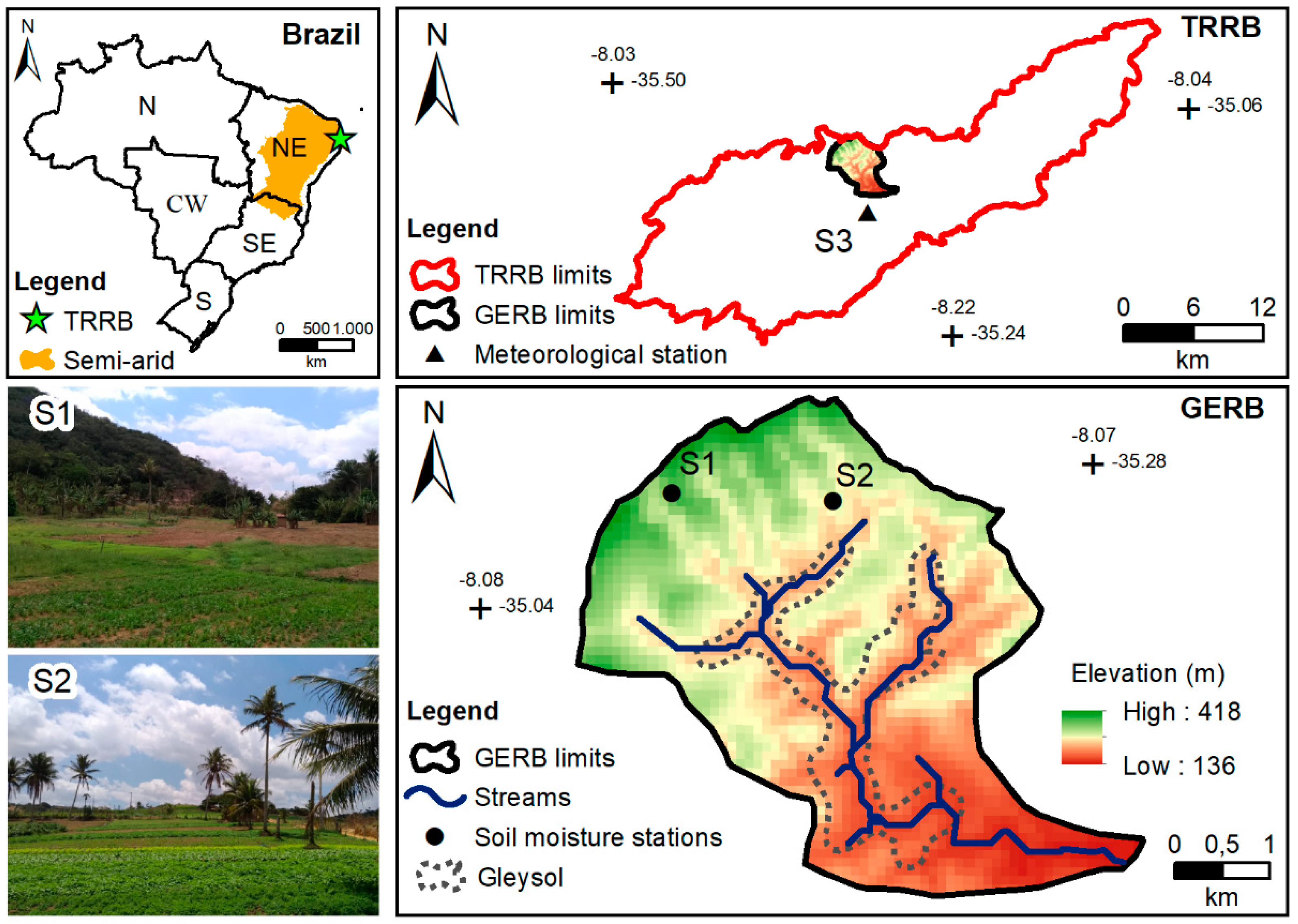
2.1. Study Site Description

This study was carried out in Gameleira Experimental River Basin (GERB), Pernambuco state, Northeast Brazil (Figure 1). The experimental basin covers 17 km² between the coordinates 8°04′ and 8°06′ S and 35°17′ and 35°20′ W. GERB is a sub-basin of the Tapacurá Representative River Basin (TRRB), which plays an important role in water supply and flood control for the Recife Metropolitan Region (RMR) [46], the fourth largest urban area in Brazil, hosting four million inhabitants. The experimental and representative catchments have been monitored by the Network of Hydrology of the Semi-Arid Region (REHISA), which currently consists of eight federal universities in Brazil [47]. In the last years, the hydrology of the GERB has been studied with regard to surface runoff [48], sediment yield [49,50], hydrodynamic soil characterization [51], and evapotranspiration [52,53].

GERB is strategically located near the transition zone between the humid (Atlantic Forest, tropical woodland) and the semi-arid zone (Caatinga, scrub vegetation). The study site is mostly covered by irrigated sugarcane and vegetable crops, evidencing the necessity of practical and precise studies considering information on the water-soil system in the region. Secondary natural vegetation and grassland for extensive cattle-raising are also found in GERB. According to Köppen’s classification proposed by Alvares et al. [54] for the Brazilian territory, the climate in GERB is tropical with dry summer (As), with an average temperature above 23 °C. The average annual rainfall in the experimental basin is approximately 1050 mm, most of which is concentrated from March to July, when the relative air humidity is higher than 70% [46].

The catchment altitude ranges between 140 and 430 m above sea level, with many points presenting high slopes. The dominant soil types in GERB are Acrisols and Gleysols, according to the WRB 2006 [55]. Acrisols are well drained, with structure developed in blocks and a large percentage of silt in their composition. On the other hand, Gleysols occur at the banks of the watercourses and are characerized by a low coefficient of infiltration when saturated and low hydraulic conductivity [56].

2.2. Data Collection

Soil moisture data were automatically measured at two monitoring stations (S1 and S2, Figure 1) by using TDR probes (CS616, Campbell Scientific). Data from monitoring stations S1 and S2 were collected between March 2014 and December 2016. One TDR probe per site was vertically inserted in the soil to indirectly represent the average water content along the first 30 cm downward from the surface, i.e., over the depth of 0–30 cm. The two TDR probes were calibrated in the laboratory, with the reproduction of the field conditions in soil column tests.

Table 1. Physical properties of the soil at the monitoring stations.

Site	Soil Type	Depth (cm)	Soil Particle Composition			Bulk Density	Particle Density
			Sand (%)	Silt (%)	Clay (%)	(g cm−3)
S1	Acrisol	0–10	71.61	20.06	8.33	1.54	2.62
		10–20	71.72	18.68	9.60	1.50	2.60
		20–30	76.14	14.11	9.75	1.51	2.58
S2	Acrisol	0–10	67.56	24.01	8.43	1.58	2.58
		10–20	60.40	21.26	18.34	1.62	2.56
		20–30	65.88	23.10	11.02	1.64	2.58

shows some soil characteristics of monitoring stations S1 and S2, such as the soil type, textural characterization, bulk density, and particle density. Overall, these two sites present similar physical properties of the soil and homogeneity of the profiles along the depths of 0–10, 10–20, and 20–30 cm. During the rainy season, the groundwater levels are approximately 1 and 4 m above the soil surface in stations S1 and S2, respectively. Both monitored sites are covered by sparse grass frequently trimmed, with root depth inferior to 10 cm.

Daily meteorological data were also used in this study to calculate the potential evapotranspiration (ET_p) by Penman’s formulation [57] modified by Shuttleworth [58]. This formulation is a physically-based form of ET_p, which means that all key variables that govern the evaporative process are explicit in the equation [59]. Donohue et al. [60] demonstrated that this form of ET_p is the most appropriated when considering a changing climate, which was also used by Coelho et al. [61] in a study carried out in the Brazilian Northeast region. The data necessary to calculate the ET_p by the Penman’s formulation were acquired from a meteorological station (named S3) operated by Pernambuco Water and Climate Agency (APAC). Meteorological station S3 is approximately 6 km from stations S1 and S2 and automatically monitors the following variables: rainfall, air temperature, relative humidity, atmospheric pressure, wind speed, and solar radiation. In addition, rainfall data were also obtained by using two automatic rain gauges installed in stations S1 and S2.

2.3. Modelling the Unsaturated Water Flow

Unsaturated water flow in GERB was modelled using the Hydrus-1D package, a free modelling environment that allows the simulation of water, heat, and solute transport in variably saturated media under permanent or transient regimes [28]. The governing equation of one-dimensional water flow for a partially saturated porous medium can be described by a modified form of the Richards equation [26], as described in Equation (1). The application of this modified form assumes that the air phase plays an insignificant role in the liquid flow process and the water flow due to thermal gradients, and therefore they can be neglected [62].

$$\frac{\partial \theta }{\partial t}=\frac{\partial }{\partial z}\left[K\left(h\right)\left(\frac{\partial h}{\partial z}+1\right)\right]-S\left(h\right)$$

(1)

where h is the water pressure head (cm), θ is the volumetric water content (cm³ cm⁻³), t is time (day), x is the vertical coordinate axis (cm) (positive upward), K(h) is the hydraulic conductivity (cm day⁻¹), and S(h) is the sink term in the flow equation (cm³ cm⁻³ day⁻¹), which represents the root water uptake (actual transpiration), obtained using the Feddes equation (more information can be found in the manual [28]). K(h) and θ(h) are obtained from the following functions according to van Genuchten [63]:

$$\theta \left(h\right)={\theta }_r+\frac{{\theta }_s-{\theta }_r}{{\left[1+{\left|\alpha h\right|}^n\right]}^m}, h<0$$

(2)

$$\theta \left(h\right)={\theta }_s, h\ge 0$$

(3)

$$K\left(h\right)=K_s{S}_e^l{\left[1-{\left(1-S_e^{1/m}\right)}^m\right]}^2$$

(4)

where θ_r is the residual water content (cm³ cm⁻³), θ_s is the saturated water content (cm³ cm⁻³), K_s is the saturated hydraulic conductivity (cm day⁻¹), l is the shape factor in the hydraulic conductivity function (assumed to be equal to 0.5), m, α, and n are empirical shape factors in the water retention function (m = 1 − 1/n), and S_e is the relative saturation, calculated as follows:

$$S_e=\frac{\theta -{\theta }_r}{{\theta }_s-{\theta }_r}$$

(5)

2.4. Estimation of Soil Hydraulic Parameters Using BEST Methods

The soil hydraulic parameters required for the Hydrus-1D simulation were obtained by the BEST method [64]. The BEST method has wide advantages when compared to other classical methods because it provides a complete characterization of both soil water retention and hydraulic conductivity functions. BEST is based on the van Genuchten [63] relationship for the water retention curve, by using the Burdine [65] condition and the Brooks and Corey [66] relationship for hydraulic conductivity (Equation (6) [65]) and Equation (7). These relationships were used because Fuentes et al. [67] found they gave more accuracy when describing the hydraulic behaviour of most soil types analyzed.

$$\frac{\theta -{\theta }_r}{{\theta }_s-{\theta }_r}={\left[1+{\left(\frac{h}{h_g}\right)}^n\right]}^{-m} \mathrm{with} m=1-\frac{2}{n}$$

(6)

$$\frac{K\left(\theta \right)}{K_s}={\left(\frac{\theta -{\theta }_r}{{\theta }_s-{\theta }_r}\right)}^{\eta }$$

(7)

where h_g is the scale parameter (cm) of θ(h), and η is the shape parameter of the K(θ) relationship. Usually, θ_r is very low and is assumed to be zero in BEST. The saturated water content (θ_s) is derived from the value of bulk density, being assumed to be equal to the porosity. This set of formulae for water retention and hydraulic conductivity functions is referred to as the vGBC functions (van Genucthen–Brooks and Corey functions).

BEST methods require two sets of data to estimate all the hydraulic parameters: (i) the Particle-Size Distribution (PSD) of the soil and bulk density and (ii) cumulative infiltration along with the initial and final soil water contents of the infiltration experiment [40,41]. Three algorithms were developed to analyze the infiltration data: (i) the original version, namely BEST-slope [41], (ii) an improved method for coarse media, namely BEST-intercept [68], and (iii) a third method, BEST-steady [69], based on the analysis of the last part of the cumulative infiltration [40]. The difference between the three methods lies in the way in which the cumulative infiltration data are processed. In this study the BEST-slope and BEST-intercept algorithms were used; however, the results of the first algorithm were discarded due to divergent values of K_s. According to Yilmaz et al. [68], the BEST-slope may lead to erroneous values of K_s, especially when a very high level of precision relative to the steady-state infiltration rate cannot be obtained.

In this study, the infiltration experiments were performed at depths of approximately 10 cm from the soil surface in order to represent the range of soil moisture obtained by the probes installed in the field. For the experiments, fixed water volumes (70 mL) were poured into a 75-mm-diameter ring, leading to a ponded water thickness of a few millimetres. Three infiltration experiments were performed at each of the monitoring stations S1 and S2 to improve the representativeness of the site. The time required for the infiltration of each water volume was measured until steady state was reached and the surface soil was sampled at the end of each experiment. These collected samples were used to determine the final profiles of θ_s and to analyze the particle size of the soils, as previously done by Coutinho et al. [40]. Although BEST assumes that θ_r is equal to zero, the value of this parameter was determined in the laboratory and fixed for the initial model simulations.

The shape parameters n, m, and η are derived from the pedotransfer functions detailed in BEST [41]. Then, the cumulative infiltrations are treated and fitted to the models developed for water infiltration into the disc source by Haverkamp et al. [38] to derive the field-saturated soil hydraulic conductivity (K_s) and soil sorptivity (S). The scale parameter for the water retention curve, hg, is then obtained from the estimates of K_s and S. In this step, all unsaturated hydraulic parameters, namely θ_r, θ_s, n (and thus m), η, h_g, and K_s, are fully estimated and the complete water retention and hydraulic conductivity functions are determined [40,41].

The retention curve parameters obtained by the BEST method were adjusted in this study because the Hydrus-1D model uses the van Genuchten equation with the Mualem [70] pore distribution condition. Therefore, the Retension Curve (RETC) program elaborated by van Genuchten et al. [71] was used. RETC uses the parametric models of vGBC functions to fit the hydraulic curves previously determined with BEST. After adjusting the retention curve, the parameters α = 1/h_g (cm⁻¹) and a new value of n were obtained.

2.5. Boundary Condition

For the atmosphere boundary condition, the variable flow of daily precipitation and potential evapotranspiration were used, considering free drainage for the lower boundary condition. Hydrus-1D requires separated input values of both potential evaporation (the upper boundary condition) and potential transpiration (the sink term in the Richards equation) fluxes at a daily time step to simulate the influence of soil water on transpiration (root water uptake) [62]. Then, potential evaporation (E_p) and potential transpiration (T_p) were separated according to the model based on the Leaf Area Index (LAI) using Beer’s law [72] as follows:

$${\mathrm{T}}_{\mathrm{p}}={\mathrm{ET}}_{\mathrm{p}}\left[1-e^{\left(-k \mathrm{LAI}\right)}\right]$$

(8)

$${\mathrm{E}}_{\mathrm{p}}={\mathrm{ET}}_{\mathrm{p}}{e}^{\left(-0.463 \mathrm{LAI}\right)}$$

(9)

where k is an extension coefficient for global solar radiation and depends on the angle of the sun, the distribution of plants, and the arrangement of leaves [62,73]. In this study, we adopted the same k-value of 0.463 that was considered by Chen et al. [13] and Šimůnek [28]. The value of LAI was assumed to be equal to 1.0 and constant for the whole period of simulation because S1 and S2 are installed in a sparse lawn area. This constant LAI with time is the same used by Chen et al. [13], which selected values in a feasible range for grasses and found LAI = 1 the more consistent after optimization and calibration of the parameters. The partitioned daily values of ET_p were then used as input data for the model (Figure 2).

2.6. Time and Space Discretisation

Regarding the geometry of the numerical domain, we considered a profile with a depth of 60 cm composed of a single control layer (corresponding to the physical and hydrodynamic properties obtained in the infiltration test performed for the 10 cm layer). This assumption of a homogeneous soil along the first 60 cm of the profile was considered after the collection of samples for soil characterization, where the same structural class was found. The numerical domain is made of a compact mesh of 201 nodes. Daily time discretisation was used in this study, with the initial time considered as 0 (the day before the simulation) and the final time referring to the days for calibration and validation. The soil moisture measured on the day before the simulation start was used as the initial condition. For the convergence criteria, the maximum number of 10 iterations for the resolution of the Richards non-linear equation was chosen, with a value of 0.001 for the tolerance of the water content in the unsaturated region of the nodes, in agreement with the default values [28]. As mentioned above, the hydraulic curves were described using the van Genuchten model for the water retention curve [63], with the Mualem condition, and the Mualem model for hydraulic conductivity. This set of formulae for water retention and hydraulic conductivity functions is referred to as the vGM functions. We did not consider the hysteresis phenomenon.

2.7. Simulations of Volumetric Water Content and Model Evaluation

The simulations were started with the hydraulic parameters obtained by the BEST method and adjusted to the vGM formulations for the period of two years. Then, optimization of the hydraulic parameters was performed by inverse modelling with the model parameters adjusted to minimize the difference between observed and simulated values [74]. The parameter algorithm employed by the Hydrus-1D model for optimization purposes is based on the Marquardt-Levenberg method [28]. The optimization was performed by using 365 and 268 days throughout 2015 for S2 and S1, respectively. A reduced number of days was used for this purpose at S1 because the station only started to operate at the end of March 2015.

On the other hand, the year 2016 was used for the validation of the model, performed soon after the calibration of the hydraulic parameters. Three statistical criteria were adopted to analyze the performance of the model: (i) the root mean square error (RMSE); (ii) the Willmott index (d); and (iii) the Nash-Sutcliffe model efficiency coefficient (NSE).

$$\mathrm{RMSE} =\sqrt{\frac{1}{\mathrm{n}}\left[{\displaystyle \sum }_{\mathrm{i}=1}^{\mathrm{n}}{\left({\theta }_o-{\theta }_m\right)}^2\right]}$$

(10)

$$\mathrm{d}=1-\frac{{\sum }_{\mathrm{i}=1}^{\mathrm{n}}{({\theta }_m-{\theta }_o)}^2}{{\sum }_{\mathrm{i}=1}^{\mathrm{n}}\left(\left|{\theta }_m-\overline{\theta }\right|+\left|{\theta }_o-\overline{\theta }\right|\right)}$$

(11)

$$\mathrm{NSE}=1-\frac{{\sum }_{\mathrm{i}=1}^{\mathrm{n}}{\left({\theta }_o-{\theta }_m\right)}^2}{{\sum }_{\mathrm{i}=1}^{\mathrm{n}}{\left({\theta }_o-\overline{\theta }\right)}^2}$$

(12)

where θ_o and θ_m are the observed and modelled soil moisture values, respectively, $\overline{\theta }$ is the mean of the observed moisture values, and n is the number of comparable paired points.

3. Results and Discussion

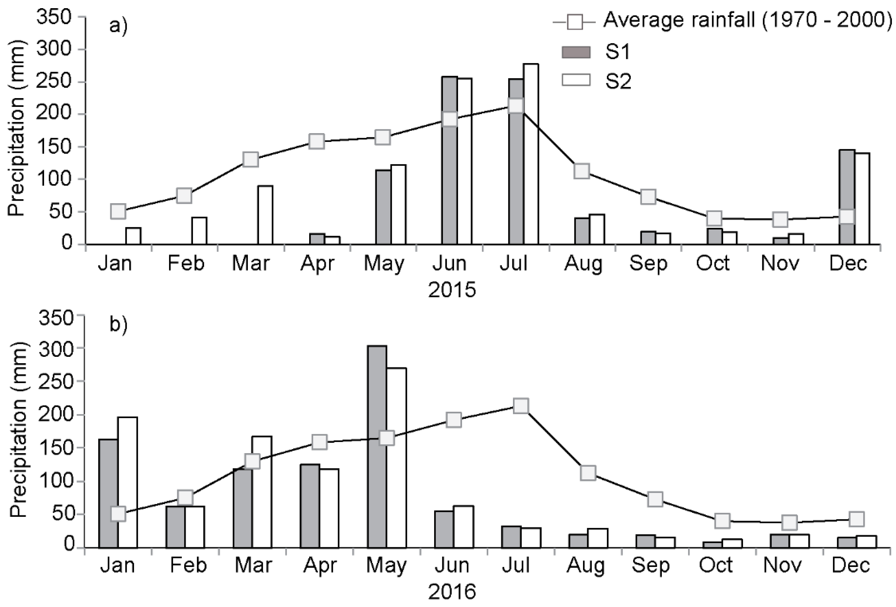
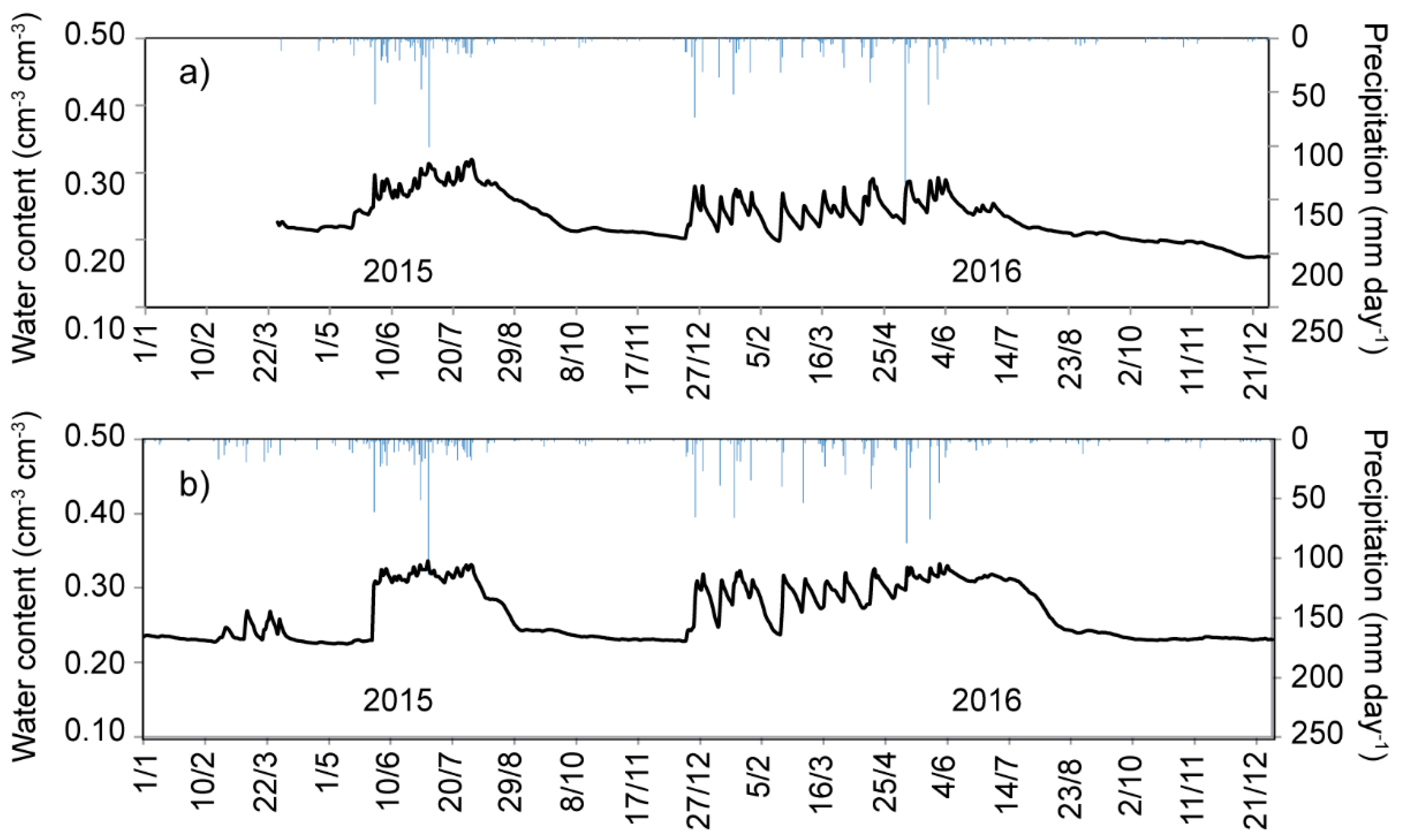
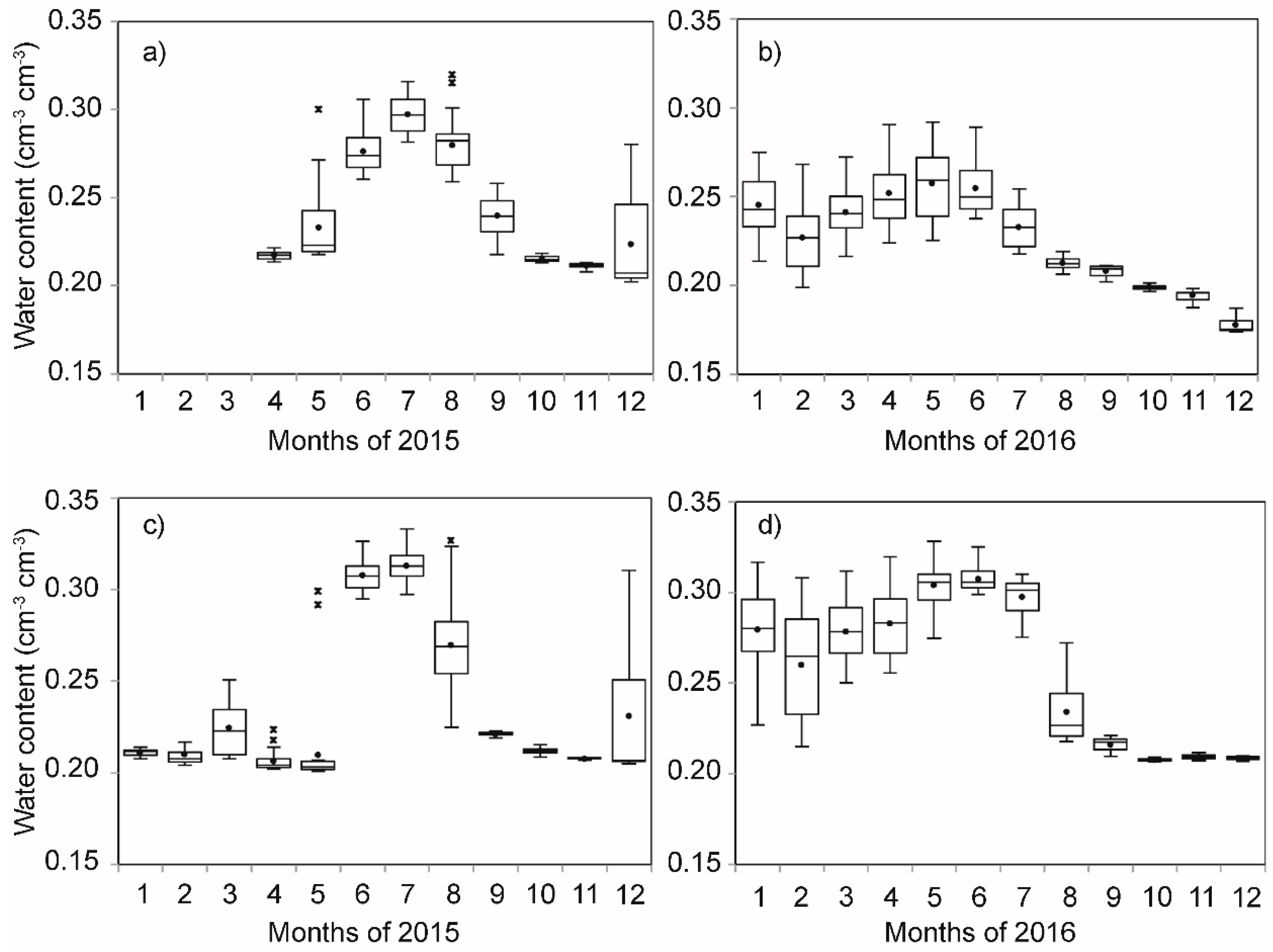
3.1. Rainfall and Soil Moisture Dynamics

Figure 3 shows the differences between monthly rainfall regimes in the two studied hydrological years and the average monthly rainfall time series from 1970 to 2000 in the Tapacurá representative river basin, TRRB. In 2015, the rainy period occurred between March and July as well as in December. On the other hand, the rainfall was more concentrated from January to May in 2016, which does not correspond to the rainy period registered in the monthly long-term time-series for TRRB [75]. In the two analyzed years, the precipitation in GERB was around 20% less than the annual average for the region, with values of 1821 and 2060 mm registered for S1 and S2, respectively.

The time series of volumetric water content (Figure 4) were obtained based on the calibration curves of CS616 probes performed in the laboratory. Analysing the soil moisture behaviour as a function of precipitation, it is observed that rainfall events above 15 mm generally provide rapid responses in the two stations. The highest increases in soil water content occurred during the rainfall events observed from May to July 2015, with maximum values of 0.32 and 0.33 cm³ cm⁻³ in S1 and S2, respectively. After the abrupt increase of soil moisture at the end of May 2015, which was influenced by a rainfall event of 61 mm, the water content in the soil remained slightly stable in S1 and S2 until the end of the rainy period in July. In 2016, the soil moisture variability was higher than in 2015 during the rainfall events, exhibiting many abrupt increases and decreases in soil water content. These different soil moisture temporal patterns are probably associated with the divergent behaviour of rainfall between the two analyzed years. While in 2015, the rainy season was more concentrated and without the presence of abrupt decreases of soil moisture, throughout the year 2016, the rain was sparser during the rainy season and consequently depletions in the soil moisture were smoother in the two stations. After the rainy period, the water content in the soil presented a mild depletion during the first days of August in both analyzed years, that is, at the beginning of the dry season. These decreases after the rainy season are more pronounced at S2, probably due to the surrounding vegetation slightly lower, and tend to stabilize at values close to 0.20 cm³ cm⁻³.

Figure 5 shows box plots with the variability and distribution of the observed mean daily soil moisture (the dot inside the box) for each month at the two monitoring stations, and the median (central marks), minimum, and maximum are also presented. The box delimits the lower and upper quartiles and outliers. The presence of outliers was only noted in 2015 due to the higher values of soil moisture, probably caused by isolated rainfall events. The isolated rainfall events observed in 2015 generated more accentuated increases in soil water content, differing from the other events. The presence of these atypical values can also be associated with the beginning and ending of the rainy season, as observed in May and August.

The highest dispersion of data is observed in the transition months between dry–wet and wet–dry periods, such as August and December 2015 and the first semester of 2016, and during the wetter periods. This variability can be noted from the difference between maximum and minimum values as well as the distance between the quartiles and the median. On the other hand, the driest months presented the lowest variability of data, as expected due to the absence of high rainfall volumes. These lowest variabilities were observed from September to October 2015 and after the end of the rainy season in 2016 (starting in August).

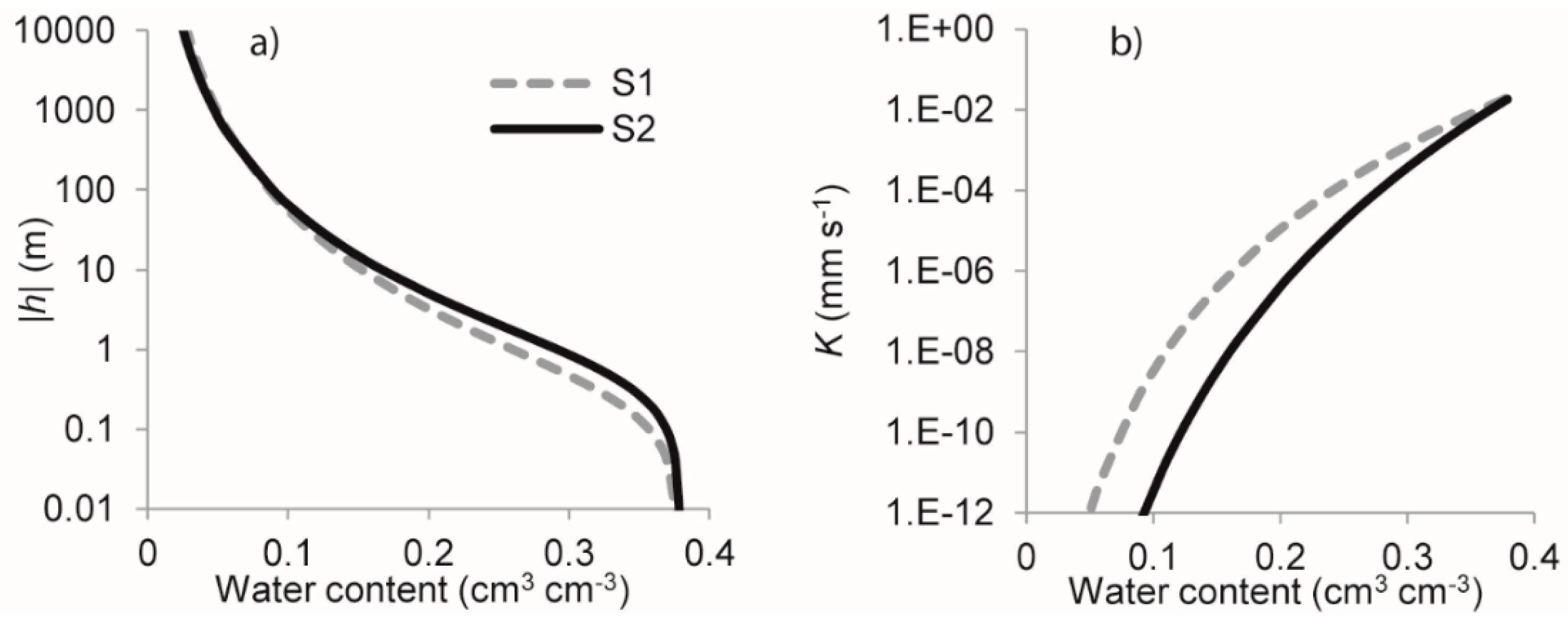
3.2. Hydraulic Characterization of the Sites

Table 2. Mean values of the hydraulic parameters derived from Beerkan Estimation of Soil Transfer (BEST) and Retension Curve (RETC) of the three replicates performed at each station.

Site	BEST Output								RETC Output
	m	n	η	S (mm s−1/2)	Ks (cm day−1)	θr1 (cm3 cm−3)	θs (cm3 cm−3)	hg (cm)	A (cm−1)	n
S1	0.102	2.223	11.482	1.31	159.97	0.063	0.377	−18.5	0.041	1.245
S2	0.094	2.204	12.682	1.20	155.52	0.026	0.379	−16.7	0.020	1.273

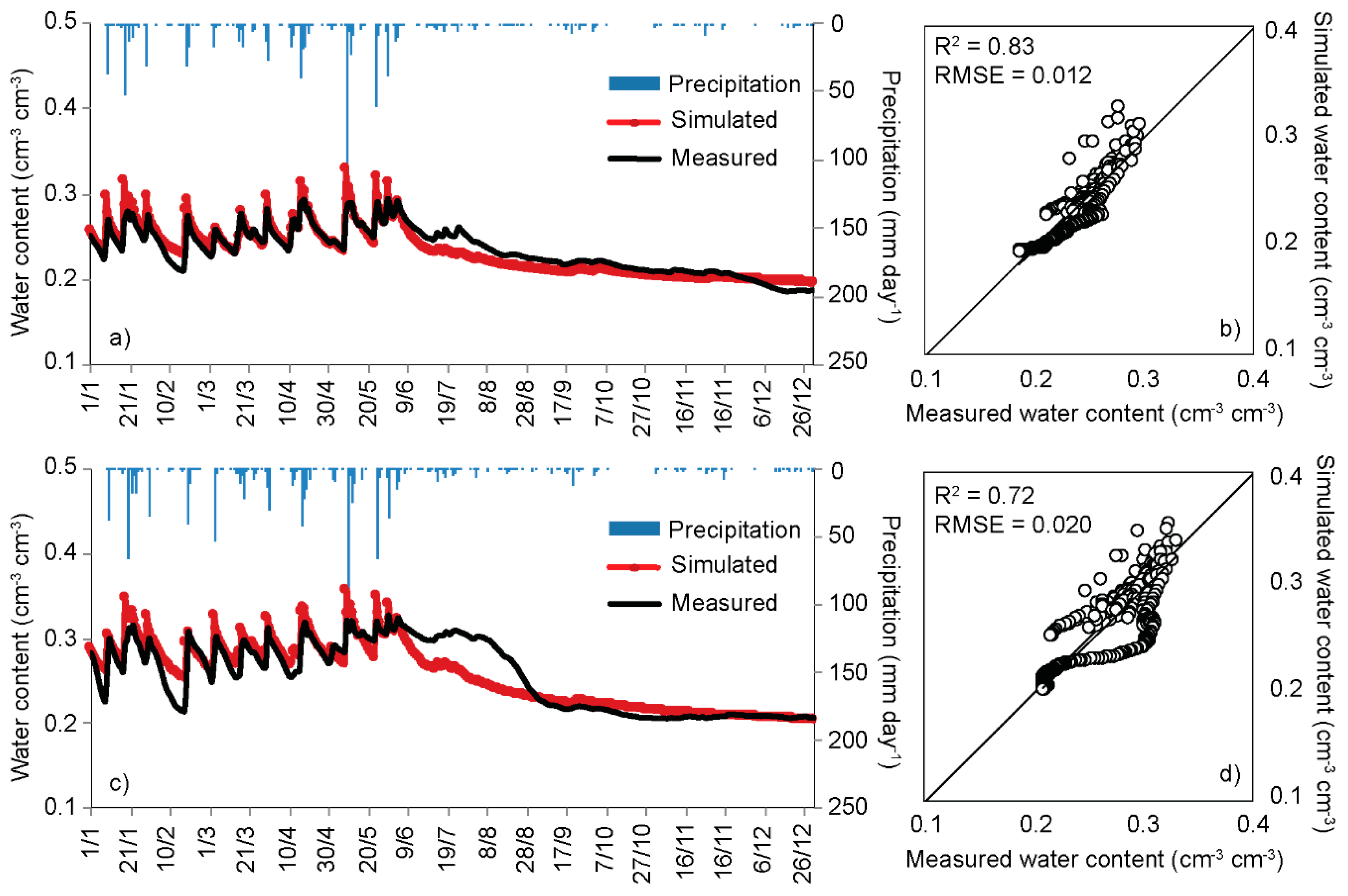
¹ The value of θ_r was measured in the laboratory.

presents the results of the mean values of the shape (m, n, and η) and normalisation (S, K_s, θ_s, and h_g) parameters of the soils generated by the BEST method for stations S1 and S2. Adjusted parameters (α and n) for the vGM functions using the RETC program are also exhibited in Table 2. The parameters m and n, which depend on the soil texture, presented the highest values in the soil with the sandiest fraction, that is, at station S1. The shape parameters strongly depend on the type of soil, with higher values of parameters n and m for the coarser materials (sand and silty sand) and smaller values of the parameter η for coarse soils [40,76]. The soil at station S1 also exhibits slightly higher values of S and K_s. The estimated values are similar to the results found by Furtunato et al. [51], who also used the BEST method at 102 points distributed throughout the GERB.

Figure 6 shows the hydraulic conductivity and water retention curves of the soils at stations S1 and S2 obtained from the mean values of the hydraulic parameters. The water retention curves were fitted to the vGM functions, generating the new parameters α and n (Table 2).

Accordingly, a similar hydraulic behaviour was verified between the soils present at the studied stations. Both hydraulic curves present an accentuated format typical of coarser materials, with a very marked inflexion point before saturation. This similarity of shapes is in agreement with the proximity of the adjusted values of the parameter n in the two soils (Table 2), as this parameter mainly determines the slope of the retention curve at larger potential values [77]. In this case, water retention is mainly affected by the soil texture [78], which is similar in the two stations (see Table 1). It is possible to observe that the Ks values at station S1 are higher than those noted at S2 for almost all ranges of soil water content. The values of K at the two stations only reach similar amounts when the soils are near to saturation (~ 160 cm day⁻¹).

3.3. Simulation

The first simulations were performed with the hydraulic parameters estimated by the BEST method and adjusted to vGM functions (Table 2). The results of the simulation at both station S1 and station S2 present similar tendencies of variation, with estimated soil moisture values close to the observed data in almost the entire series throughout the studied period (Figure 7). Exceptions are noted during the dry periods, especially in S2, when the simulated data cannot effectively capture the observed recession curves. This may have been influenced by the lower boundary condition adopted in the simulation, which in this case was free drainage disregarding the depth of the groundwater. It is possible that in the field there is a small contribution of capillarity to soil moisture. Another possible explanation for the underestimated results of the model at the two sites may be the constant value considered for LAI over the whole simulation, promoting periods with higher evaporation rates and consequently reducing soil moisture rates.

The scatter plots also show the good agreement between observed and estimated data, with values of R² ranging from 0.72 (S1) to 0.81 (S2) and RMSE below 0.024 cm³ cm⁻³ (Figure 7b,d). Honari et al. [36] used the soil parameters estimated by the BEST method to evaluate the performance of Hydrus-3D model in simulating 3D water flow and water content in a short time period and at different depths of a soil cultivated with corn and durum in Montpellier, France. They also obtained good results without parameter calibration, with RMSE values between 0.0174 and 0.019 cm³ cm⁻³. The authors emphasized that the quality of hydrodynamic property estimates is fundamental for accuracy in simulations.

Some studies used hydraulic parameters estimated by the Rosetta Lite pedotransference function [79] to start the simulations of the behaviour of water in the vadose zone using Hydrus-1D [30,32,33,73]. By analysing the efficiency of this function, Okamoto et al. [80] observed that the hydraulic parameters measured in the field presented better results than those estimated by Rosetta Lite. They highlighted the importance of the use of measured parameters when simulating the water flux in the unsaturated zone. The results found at this step demonstrate the good efficiency of hydrodynamic parameters determined in situ with the BEST model, adjusted by the RETC, to characterize the temporal variability of soil moisture in the GERB.

Table 3. Calibrated soil hydraulic parameters by using the inverse solution for the monitoring stations.

Site	θr (cm3 cm−3)	θs (cm3 cm−3)	α (cm−1)	n	Ks (cm day−1)	l
S1	0.107	0.342	0.037	1.23	234.2	0.5
S2	0.056	0.369	0.018	1.17	243.7	0.5

presents the hydraulic parameters of the soil calibrated by inverse modelling. After calibration, residual moisture values increased and saturated moisture decreased in the two stations. The saturated hydraulic conductivity in the two stations increased approximately 50% of predicted values using the BEST methods (Table 2 versus Table 3). Chen et al. [13] used Hydrus-1D to simulate soil moisture in two sub-basins of the Goulburn River, Australia, for a period of three years. They observed that inverse modelling modified the soil properties, reducing the values of θ_r while θ_s and K_s increased. According to the aforementioned authors, the calibrated hydraulic parameters represent, in addition to soil texture, factors such as the number of macropores caused by roots or cracks, vegetation type, organic matter, and anthropic activities.

Figure 8 shows the results of the modelling validation. It is noticeable that the estimated soil water content is better adjusted to the observed values obtained in situ. However, a discrepancy between the observed and estimated data remains in both stations after the end of the rainy season. At S1, the simulated data follow the same pattern of the measured soil moisture variation; however, the model slightly overestimated the measured values for some rainfall events (Figure 8a). For instance, the response of the model to the rainfall of 133.8 mm that occurred on 9 May 2016 was 0.33 cm³ cm⁻³, while the observed value registered was 0.27 cm³ cm⁻³. For the same station, the model was unable to detect the rainfall events that occurred from 13 June 2016 to 10 August 2016, underestimating the measured soil moisture data.

The simulated data for S2 also presented overestimated values for some rainfall events (Figure 8). Similar underestimation was also observed after the rainy season from 10 July 2016 to 9 August 2016, with a considerable difference between the observed and estimated data. This behaviour of the model in underestimating the observed data is probably linked to the high infiltration rate considered by Hydrus-1D, which is larger than that which actually occurs with the antecedent soil moisture.

The correlation between estimated and simulated values for the two monitoring stations is shown in Figure 8b,d. The dispersion between the data indicates that the observed soil water content is represented well by the modelling results, with R² values equal to 0.83 (S1) and 0.72 (S2). Silva et al. [29] obtained similar values of R² (0.79 for natural cover and 0.78 for bare soil) by using the Hydrus-1D model to simulate soil moisture in an Acrisol in Brazil using 151 days of the year 2013 for validation. The authors attributed the results obtained to the different hydrological behaviours between the years used for calibration and validation, particularly the changes in interception rate and evapotranspiration and the scarcity of rainfall events in the calibration period. Any change in vegetation or soil structure at the surface may impact the water budget, mainly the runoff and infiltration processes.

Figure 8b,d also shows that some points are still far from the straight 1:1 line for the two stations, even though R² presents good values. This occurred because of the response of the model to some isolated rainfall events, which raised the soil moisture to values higher than those measured in the field. Another divergent behaviour is observed below the 1:1 line, where the model failed to respond to the small rainfall events that occurred in June and July after the rainy season, underestimating the soil moisture values measured in the field.

Another possible cause of the observed divergence between simulated and observed values is associated with some possible small errors that accumulated throughout the data acquisition process, such as: (i) characterization of soil properties, (ii) calibration of the sensors in the laboratory, and (iii) some criteria adopted for simulation of the model (e.g., LAI and lower boundary condition), as previously described.

Table 4. Hydrus-1D model goodness of fit and accuracy. RMSE: Residual Mean Square Errors; d: Willmott coefficient of agreement; NSE: Nash-Sutcliffe model efficiency coefficient.

Site	RMSE (cm3 cm−3)	d	NSE
S1	0.012	0.95	0.783
S2	0.020	0.93	0.740

presents the results of the performance evaluation of the model. The RMSE for the simulated and observed soil moisture data exhibited good absolute values equal to 0.012 and 0.020 cm³ cm⁻³ for S1 and S2, respectively. The Willmott coefficient of agreement (d) close to 1 also evidences the good accuracy of the soil moisture simulations under the investigated conditions. The NSE values for the simulations at both station S1 and station S2 were classified as being “very good” (0.75 < NSE < 1) and “good” (0.65 < NSE ≤ 0.75), respectively. These results are similar to those found by Silva et al. [29] using Hydrus-1D for simulations, with d equal to 0.93 and 0.94 and NSE equal to 0.72 and 0.74 for natural and bare soils, respectively.

The comparison between simulated and validated results shows that the RMSE values were very close, with a small reduction of 0.009 cm³ cm⁻³ at S1 and a of 0.002 cm³ cm⁻³ at S2 (see Figure 7 and Figure 8). Considering the aforementioned results and the entire time series used in both the initial simulation and the validation (2015 and 2016), it can be noticed that the parameters estimated by the BEST method are efficient for use in the Hydrus-1D model and describe the soil conditions in the GERB well, without the need for calibration. Therefore, simplified estimates of soil properties by the BEST method, associated with meteorological data and using Hydrus-1D model, can provide acceptable predictions of soil water content in GERB.

4. Conclusions

This study was conducted in an experimental basin in Brazil to investigate the behaviour and prediction of soil water content dynamics in the region using field measurements and numerical methods. Soil moisture presented the greatest and the lowest variability during the rainy transitions (dry–rainy–dry) and dry periods, respectively. The soil water content did not approximate the residual and saturation contents throughout the period. The Hydrus-1D model adequately simulated the soil moisture variability both with the parameters estimated by the BEST model and after their calibration (numerical optimization of parameters by fitting experimental measures). Indeed, these optimized parameters reduced the differences between the measured and simulated values, as expected. However, the inverse modelling requires a considerable number of observations, which means it is limited to well monitored basins. Meanwhile, the gain in accuracy was not drastic, suggesting that BEST estimates were sufficient. Thus, the performance analysis of the simulations provided strong indications of the efficiency of parameters estimated by BEST to predict the soil moisture variability in the studied region, without the need for calibration or complex numerical approaches. This result indicates that the BEST method can be adequate for depicting the water retention and hydraulic conductivity functions, even with the final aim of modelling the water flow processes and water budget for a soil profile. It must be mentioned that the approach was based on the modelling of a soil profile, considering a uniform soil. The impact of soil heterogeneity and spatial variability of soil hydraulic characteristics in different layers of the soil profile should be investigated and the resulting flow heterogeneity should be accounted for. This issue will be the object of further investigations.

References

1. Šípek, V.; Tesar, M. Soil moisture simulations using two different modelling approaches. Die Bodenkult. 2013, 64, 99–103. [Google Scholar]
2. Bordoni, M.; Bittelli, M.; Valentino, R.; Chersich, S.; Persichillo, M.G.; Meisina, C. Soil water content estimated by support vector machine for the assessment of shallow landslides triggering: The role of antecedent meteorological conditions. Environ. Model. Assess. 2018, 23, 333–352. [Google Scholar] [CrossRef]
3. Zarlenga, A.; Fiori, A.; Russo, D. Spatial variability of soil moisture and the scale issue: A geostatistical approach. Water Resour. Res. 2018, 54, 1765–1780. [Google Scholar] [CrossRef]
4. Rodriguez-Iturbe, I.; Porporato, A. Ecohydrology of Water-Controlled Ecosystems: Soil Moisture and Plant Dynamics, 1st ed.; Cambridge University Press: Cambridge, UK, 2005. [Google Scholar] [CrossRef]
5. Sheikh, V.; van Loon, E.E. Comparing performance and parameterization of a one-dimensional unsaturated zone model across scales. Vadose Zone J. 2007, 6, 638–650. [Google Scholar] [CrossRef]
6. Ojha, R.; Morbidelli, R.; Saltalippi, C.; Flammini, A.; Govindaraju, R.S. Scaling of surface soil moisture over heterogeneous fields subjected to a single rainfall event. J. Hydrol. 2014, 516, 21–36. [Google Scholar] [CrossRef]
7. Dirmeyer, P.A.; Gao, X.; Zhao, M.; Guo, Z.; Oki, T.; Hanasaki, N. GSWP-2: Multimodel analysis and implications for our perception of the land surface. Bull. Am. Meteorol. Soc. 2006, 87, 1381–1397. [Google Scholar] [CrossRef]
8. Li, S.; Liang, W.; Zhang, W.; Liu, Q. Response of soil moisture to hydro-meteorological variables under different precipitation gradients in the Yellow River basin. Water Resour. Manag. 2016, 30, 1867–1884. [Google Scholar] [CrossRef]
9. Melo, O.R.; Montenegro, A.A.A. Dinâmica temporal da umidade do solo em uma bacia hidrográfica no semiárido pernambucano. Rev. Bras. Recur. Hídr. 2015, 20, 430–441. [Google Scholar] [CrossRef]
10. Huang, X.; Shi, Z.H.; Zhu, H.D.; Zhang, H.Y.; Ai, L.; Yin, W. Soil moisture dynamics within soil profiles and associated environmental controls. Catena 2016, 136, 189–196. [Google Scholar] [CrossRef]
11. Negm, A.; Capodici, F.; Ciraolo, G.; Maltese, A.; Provenzano, G.; Rallo, G. Assessing the performance of thermal inertia and Hydrus models to estimate surface soil water content. Appl. Sci. 2017, 7, 975. [Google Scholar] [CrossRef]
12. Brocca, L.; Ciabatta, L.; Massari, C.; Camici, S.; Tarpanelli, A. Soil moisture for hydrological applications: Open questions and new opportunities. Water 2017, 9, 140. [Google Scholar] [CrossRef]
13. Chen, M.; Willgoose, G.R.; Saco, P.M. Spatial prediction of temporal soil moisture dynamics using HYDRUS-1D. Hydrol. Process. 2014, 28, 171–185. [Google Scholar] [CrossRef]
14. Tavakoli, M.; De Smedt, F. Validation of soil moisture simulation with a distributed hydrologic model (WetSpa). Environ. Earth Sci. 2013, 69, 739–747. [Google Scholar] [CrossRef]
15. Legates, D.R.; Mahmood, R.; Levia, D.F.; DeLiberty, T.L.; Quiring, S.M.; Houser, C.; Nelson, F.E. Soil moisture: A central and unifying theme in physical geography. Prog. Phys. Geogr. 2011, 35, 65–86. [Google Scholar] [CrossRef]
16. Escorihuela, M.J.; Quintana-Seguí, P. Comparison of remote sensing and simulated soil moisture datasets in Mediterranean landscapes. Remote Sens. Environ. 2016, 180, 99–114. [Google Scholar] [CrossRef] [Green Version]
17. Espejo-Pérez, A.J.; Brocca, L.; Moramarco, T.; Giráldez, J.V.; Triantafilis, J.; Vanderlinden, K. Analysis of soil moisture dynamics beneath olive trees. Hydrol. Process. 2016, 30, 4339–4352. [Google Scholar] [CrossRef]
18. Zribi, M.; Le Hégarat-Mascle, S.; Ottlé, C.; Kammoun, B.; Guerin, C. Surface soil moisture estimation from the synergistic use of the (multi-incidence and multi-resolution) active microwave ERS Wind Scatterometer and SAR data. Remote Sens. Environ. 2003, 86, 30–41. [Google Scholar] [CrossRef]
19. She, D.; Liu, D.; Xia, Y.; Shao, M. Modeling effects of land use and vegetation density on soil water dynamics: Implications on water resource management. Water Resour. Manag. 2014, 28, 2063–2076. [Google Scholar] [CrossRef]
20. Chen, B.; Liu, E.; Mei, X.; Yan, C.; Garré, S. Modelling soil water dynamic in rain-fed spring maize field with plastic mulching. Agric. Water Manag. 2018, 198, 19–27. [Google Scholar] [CrossRef] [Green Version]
21. Van Dam, J.C.; Huygen, J.; Wesseling, J.G.; Feddes, R.A.; Kabat, P.; van Walsum, P.E.V.; Groenendijk, P.; van Diepen, C.A. Theory of SWAP Version 2.0: Simulation of Water Flow, Solute Transport and Plant Growth in the Soil-Water-Atmosphere-Plant Environment; Technical Document 45; Wageningen Agricultural University and DLO Winand Staring Centre: Wageningen, The Netherlands, 1997. [Google Scholar]
22. Avissar, R. Which type of soil-vegetation-atmosphere transfer scheme is needed for general circulation models: A proposal for a higher-order scheme. J. Hydrol. 1998, 212–213, 136–154. [Google Scholar] [CrossRef]
23. Verburg, K.; Ross, P.J.; Bristow, K.L. SWIM v2.1 User Manual; Divisional Report No. 130; CSIRO Division of Soils: Canberra, Australia, 1996.
24. Leonard, R.A.; Knisel, W.G.; Still, D.A. GLEAMS: Groundwater loading effects of agricultural management systems. Trans. ASAE 1987, 30, 1403–1418. [Google Scholar] [CrossRef]
25. Vanclooster, M.; Viaene, P.; Diels, J.; Christiaens, K. WAVE: A mathematical model for simulating water and agrochemicals in the soil and vadose environment. In Reference and User’s Manual, Release 2.1; Institute for Land and Water Management, Katholieke Universiteit Leuven: Leuven, Belgium, 1996. [Google Scholar]
26. Richards, L.A. Capillary conduction of liquids through porous mediums. J. Appl. Phys. 1931, 1, 318–333. [Google Scholar] [CrossRef]
27. Tinet, A.J.; Chanzy, A.; Braud, I.; Crevoisier, D.; Lafolie, F. Development and Evaluation of an Efficient Soil-Atmosphere Model (FHAVeT) based on the Ross fast solution of the Richards equation for bare soil conditions. Hydrol. Earth Syst. Sci. 2015, 19, 969–980. [Google Scholar] [CrossRef]
28. Šimůnek, J.; Šejna, M.; Saito, H.; Sakai, M.; van Genuchten, M.T. The HYDRUS-1D Software Package for Simulating the One-Dimensional Movement of Water, heat, and Multiple Solutes in Variably-Saturated Media Version 4.17; University of California Riverside: Riverside, CA, USA, 2013; pp. 1–342. [Google Scholar]
29. Da Silva, J.R.L.; Montenegro, A.A.A.; Monteiro, A.L.N.; Silva, P.V. Modelagem da dinâmica de umidade do solo em diferentes condições de cobertura no semiárido pernambucano. Rev. Bras. Cienc. Agrar. 2015, 10, 293–303. [Google Scholar] [CrossRef]
30. Lai, X.; Liao, K.; Feng, H.; Zhu, Q. Responses of soil water percolation to dynamic interactions among rainfall, antecedent moisture and season in a forest site. J. Hydrol. 2016, 540, 565–573. [Google Scholar] [CrossRef]
31. Li, Y.; Šimůnek, J.; Wang, S.; Yuan, J.; Zhang, W. Modeling of soil water regime and water balance in a transplanted rice field experiment with reduced irrigation. Water 2017, 9, 248. [Google Scholar] [CrossRef]
32. Wang, H.; Tetzlaff, D.; Soulsby, C. Modelling the effects of land cover and climate change on soil water partitioning in a boreal headwater catchment. J. Hydrol. 2018, 558, 520–531. [Google Scholar] [CrossRef]
33. Gabiri, G.; Burghof, S.; Diekkrüger, B.; Leemhuis, C.; Steinbach, S.; Näschen, K. Modeling spatial soilwater dynamics in a tropical floodplain, East Africa. Water 2018, 10, 191. [Google Scholar] [CrossRef]
34. Šimůnek, J.; van Genuchten, M.T. Using the HYDRUS-1D and HYDRUS-2D codes for estimating unsaturated soil hydraulic and solute transport parameters. In Characterization and Measurement of the Hydraulic Properties of Unsaturated Porous Media; van Genuchten, M.T., Leij, F.J., Wu, L., Eds.; University of California: Riverside, CA, USA, 1999; pp. 1523–1536. [Google Scholar]
35. Kato, C.; Nishimura, T.; Imoto, H.; Miyazaki, T. Predicting soil moisture and temperature of andisols under a monsoon climate in Japan. Vadose Zone J. 2011, 10, 541–551. [Google Scholar] [CrossRef]
36. Honari, M.; Ashrafzadeh, A.; Khaledian, M.; Vazifedoust, M.; Mailhol, J.C. Comparison of HYDRUS-3D soil moisture simulations of subsurface drip irrigation with experimental observations in the south of France. J. Irrig. Drain. Eng. 2017, 143, 1–8. [Google Scholar] [CrossRef]
37. Siltecho, S.; Hammecker, C.; Sriboonlue, V.; Clermont-Dauphin, C.; Trelo-Ges, V.; Antonino, A.C.D.; Angulo-Jaramillo, R. Use of field and laboratory methods for estimating unsaturated hydraulic properties under different land uses. Hydrol. Earth Syst. Sci. 2015, 19, 1193–1207. [Google Scholar] [CrossRef]
38. Haverkamp, R.; Ross, P.J.; Smettem, K.R.J.; Parlange, J.Y. Three-dimensional analysis of infiltration from the disc infiltrometer: 2. Physically based infiltration equation. Water Resour. Res. 1994, 30, 2931–2935. [Google Scholar] [CrossRef] [Green Version]
39. Braud, I.; De Condappa, D.; Soria, J.M.; Haverkamp, R.; Angulo-Jaramillo, R.; Galle, S.; Vauclin, M. Use of scaled forms of the infiltration equation for the estimation of unsaturated soil hydraulic properties (the Beerkan method). Eur. J. Soil Sci. 2005, 56, 361–374. [Google Scholar] [CrossRef]
40. Coutinho, A.P.; Lassabatere, L.; Montenegro, S.; Antonino, A.C.D.; Angulo-Jaramillo, R.; Cabral, J.J.S.P. Hydraulic characterization and hydrological behaviour of a pilot permeable pavement in an urban centre, Brazil. Hydrol. Process. 2016, 30, 4242–4254. [Google Scholar] [CrossRef]
41. Lassabatère, L.; Angulo-Jaramillo, R.; Soria Ugalde, J.M.; Cuenca, R.; Braud, I.; Haverkamp, R. Beerkan estimation of soil transfer parameters through infiltration experiments—BEST. Soil Sci. Soc. Am. J. 2006, 70, 521. [Google Scholar] [CrossRef]
42. Kanzari, S. Spatio-Temporal variability of the soil hydraulic properties—Effect on modelling of water flow and solute transport at field-scale. In Recent Advances in Environmental Science from the Euro-Mediterranean and Surrounding Regions; Kallel, A., Ksibi, M., Ben Dhia, H., Khélifi, N., Eds.; Springer: Cham, Switzerland, 2018; pp. 1279–1281. [Google Scholar] [CrossRef]
43. Lai, J.; Ren, L. Estimation of effective hydraulic parameters in heterogeneous soils at field scale. Geoderma 2016, 264, 28–41. [Google Scholar] [CrossRef] [Green Version]
44. Nascimento, Í.V.; de Assis Júnior, R.N.; de Araújo, J.C.; de Alencar, T.L.; Freire, A.G.; Lobato, M.G.R.; da Silva, C.P.; Mota, J.C.A.; Nascimento, C.D.V. Estimation of van Genuchten equation parameters in laboratory and through inverse modeling with Hydrus-1D. J. Agric. Sci. 2018, 10, 102. [Google Scholar] [CrossRef]
45. Graham, S.L.; Srinivasan, M.S.; Faulkner, N.; Carrick, S. Soil hydraulic modeling outcomes with four parameterization methods: Comparing soil description and inverse estimation approaches. Vadose Zone J. 2018, 17. [Google Scholar] [CrossRef]
46. Montenegro, S.M.G.L.M.; Ragab, R. Impact of possible climate and land use changes in the semi arid regions: A case study from north eastern Brazil. J. Hydrol. 2012, 434–435, 55–68. [Google Scholar] [CrossRef]
47. Montenegro, A.A.A.; Ragab, R. Hydrological response of a brazilian semi-arid catchment to different land use and climate change scenarios: A modelling study. Hydrol. Process. 2010, 24, 2705–2723. [Google Scholar] [CrossRef]
48. Araújo Filho, P.; Cabral, J. Modelagem hidrológica da bacia do riacho Gameleira (Pernambuco) utilizando TOPSIMPL, uma versão simplificada do modelo TOPMODEL. Rev. Bras. Recur. Hídr. 2005, 10, 61–72. [Google Scholar] [CrossRef]
49. Paiva, F.M.L.; Montenegro, S.M.G.L.; Salcedo, I.H.; Araújo Filho, P.F.; Srinivasan, V.S.; Silva Filho, S.L.; Azevedo, J.R.G.; Silva, R.M.; Silva, L.P. Análise do transporte de sedimentos em suspensão num pequeno curso d’água na bacia experimental do riacho Gameleira, PE. In Proceedings of the XIX Simpósio Brasileiro de Recursos Hídricos (SBRH), Maceió, Brazil, 27 November–1 December 2011; Available online: https://abrh.s3.sa-east-1.amazonaws.com/Sumarios/81/e7457e425ff7a2508f2b4bfb293cfbd9_e6315e8645bda4bec9188b7bdc137669.pdf (accessed on 17 December 2018).
50. Da Silva, R.M.; Paiva, F.M.D.L.; Montenegro, S.M.G.D.L.; Augusto, C.; Santos, G. Aplicação de Eqsuações de Razão de Transferência de Sedimentos na Bacia do rio Gameleira com Suporte de Sistemas de Informação Geográfica. In Proceedings of the XVIII Simpósio Brasileiro de Recursos Hídricos (SBRH), Campo Grande, Brazil, 22–26 November 2009; Available online: https://abrh.s3.sa-east-1.amazonaws.com/Sumarios/110/c9e2c8a28e3027a52b5b34e91b6f9b14_705324c4dd596d1379d42fc4fe927d8f.pdf (accessed on 17 December 2018).
51. Furtunato, O.M.; Montenegro, S.M.G.L.; Antonino, A.C.D.; de Oliveira, L.M.M.; de Souza, E.S.; Moura, A.E.S.S. Variabilidade espacial de atributos físico-hídricos de solos em uma bacia experimental no estado de Pernambuco. Rev. Bras. Recur. Hídr. 2013, 18, 135–147. [Google Scholar] [CrossRef]
52. Oliveira, L.M.M.; Montenegro, S.M.G.L. Evapotranspiração de referência na bacia experimental do riacho Gameleira, PE, utilizando-se lisímetro e métodos indiretos. Rev. Bras. Ciênc. Agrár. 2008, 81, 58–67. [Google Scholar] [CrossRef]
53. Moura, A.R.C.; Montenegro, S.M.G.L.; Antonino, A.C.D.; de Azevedo, J.R.G.; da Silva, B.B.; de Oliveira, L.M.M. Evapotranspiração de referência baseada em métodos empíricos em bacia experimental no estado de Pernambuco - Brasil. Rev. Bras. Meteorol. 2013, 28, 181–191. [Google Scholar] [CrossRef] [Green Version]
54. Alvares, C.A.; Stape, J.L.; Sentelhas, P.C.; de Moraes Gonçalves, J.L.; Sparovek, G. Köppen’s climate classification map for Brazil. Meteorol. Z. 2013, 22, 711–728. [Google Scholar] [CrossRef]
55. WRB, I.W.G. World Reference Base for Soil Resources 2006: A Framework for International Classification, Correlation and Communication; World Soil Resources Reports; Food and Agriculture Organization: Rome, Italy, 2006. [Google Scholar]
56. Braga, R.A.P. Gestão Ambiental Da Bacia Do Rio Tapacurá - Plano de Ação; Universitária-UFPE: Recife, Brazil, 2001; p. 101. [Google Scholar]
57. Penman, H.L. Natural evaporation from open water, bare soil, and grass. Proc. R. Soc. Lond. 1948, 193, 120–146. [Google Scholar] [CrossRef]
58. Shuttleworth, W.J. Evaporation. In Handbook of Hydrology; Maidment, D.R., Ed.; McGraw Hill: New York, NY, USA, 1993; pp. 4.1–4.53. [Google Scholar]
59. McVicar, T.R.; Roderick, M.L.; Donohue, R.J.; Li, L.T.; Van Niel, T.G.; Thomas, A.; Grieser, J.; Jhajharia, D.; Himri, Y.; Mahowald, N.M.; et al. Global review and synthesis of trends in observed terrestrial near-surface wind speeds: Implications for evaporation. J. Hydrol. 2012, 416–417, 182–205. [Google Scholar] [CrossRef]
60. Donohue, R.J.; McVicar, T.R.; Roderick, M.L. Assessing the ability of potential evaporation formulations to capture the dynamics in evaporative demand within a changing climate. J. Hydrol. 2010, 386, 186–197. [Google Scholar] [CrossRef]
61. Coelho, V.H.R.; Montenegro, S.; Almeida, C.N.; Silva, B.B.; Oliveira, L.M.; Gusmão, A.C.V.; Freitas, E.S.; Montenegro, A.A.A. Alluvial Groundwater Recharge Estimation in Semi-Arid Environment Using Remotely Sensed Data. J. Hydrol. 2017, 548, 1–15. [Google Scholar] [CrossRef]
62. Li, Y.; Šimůnek, J.; Jing, L.; Zhang, Z.; Ni, L. Evaluation of water movement and water losses in a direct-seeded-rice field experiment using Hydrus-1D. Agric. Water Manag. 2014, 142, 38–46. [Google Scholar] [CrossRef] [Green Version]
63. Van Genuchten, M.T. A closed-form equation for predicting the hydraulic conductivity of unsaturated soils. Soil Sci. Soc. Am. J. 1980, 44, 892–898. [Google Scholar] [CrossRef]
64. Angulo-Jaramillo, R.; Bagarello, V.; Iovino, M.; Lassabatère, L. Infiltration Measurements for Soil Hydraulic Characterization; Springer International Publishing: New York, NY, USA, 2016; ISBN 978-3-319-31786-1. [Google Scholar] [CrossRef]
65. Burdine, N.T. Relative permeability calculations from pore size distribution Data. J. Pet. Technol. 1953, 5, 71–78. [Google Scholar] [CrossRef]
66. Brooks, R.H.; Corey, A.T. Hydraulic Properties of Porous Media; Hydrology Paper 3; Colorade State University: Fort Collins, CO, USA, 1964. [Google Scholar]
67. Fuentes, C.; Haverkamp, R.; Parlange, J.Y. Parameter constraints on closed-form soilwater relationships. J. Hydrol. 1992, 134, 117–142. [Google Scholar] [CrossRef]
68. Yilmaz, D.; Lassabatère, L.; Angulo-Jaramillo, R.; Deneele, D.; Legret, M. Hydrodynamic characterization of basic oxygen furnace slag through an adapted BEST method. Vadose Zone J. 2010, 9, 107–116. [Google Scholar] [CrossRef]
69. Bagarello, V.; Di Prima, S.; Giordano, G.; Iovino, M. A test of the Beerkan Estimation of Soil Transfer Parameters (BEST) procedure. Geoderma 2014, 221–222, 20–27. [Google Scholar] [CrossRef]
70. Mualem, Y. A new model for predicting the hydraulic conductivity of unsaturated porous media. Water Resour. Res. 1976, 12, 513–522. [Google Scholar] [CrossRef]
71. Van Genuchten, M.T.; Leij, F.J.; Yates, S.R. The RETC Code for Quantifying the Hydraulic Functions of Unsaturated Soils; Research Report n. EPA/600/2-91/065; U.S. Salinity Laboratory, USDA-ARS: Riverside, CA, USA, 1991; 93p. [CrossRef]
72. Ritchie, J.T. Model for predicting evaporation from a row crop with incomplete cover. Water Resour. Res. 1972, 8, 1204–1213. [Google Scholar] [CrossRef]
73. Qu, W.; Bogena, H.R.; Huisman, J.A.; Martinez, G.; Pachepsky, Y.A.; Vereecken, H. Effects of soil hydraulic properties on the spatial variability of soil water content: Evidence from sensor network data and inverse modeling. Vadose Zone J. 2014, 13. [Google Scholar] [CrossRef]
74. Vereecken, H.; Huisman, J.A.; Bogena, H.; Vanderborght, J.; Vrugt, J.A.; Hopmans, J.W. On the value of soil moisture measurements in vadose zone hydrology: A review. Water Resour. Res. 2008, 44. [Google Scholar] [CrossRef] [Green Version]
75. Silva, R.M.; Silva, L.P.; Montenegro, S.M.G.L.; Santos, C.A.G. Análise da variedade espaço-temporal e identificação do padrão da precipitação na bacia do rio Tapacurá, Pernambuco. Soc. Nat. 2010, 22, 357–372. [Google Scholar] [CrossRef]
76. Souza, E.S.; Antonino, A.C.D.; Angulo-Jaramillo, R.; Netto, A.M. Caracterização hidrodinâmica de solos: Aplicação do método Beerkan. Rev. Bras. Eng. Agrícola Ambient. 2008, 12, 128–135. [Google Scholar] [CrossRef]
77. Pirastru, M.; Castellini, M.; Giadrossich, F.; Niedda, M. Comparing the hydraulic properties of forested and grassed soils on an experimental hillslope in a mediterranean environment. Procedia Environ. Sci. 2013, 19, 341–350. [Google Scholar] [CrossRef]
78. Van Genuchten, M.T.; Nielsen, D. On describing and predicting the hydraulic properties of unsaturated soils. Ann. Geophys. 1985, 3, 615–627. [Google Scholar] [CrossRef]
79. Schaap, M.G.; Leij, F.J.; van Genuchten, M.T. Rosetta: A computer program for estimating soil hydraulic parameters with hierarchical pedotransfer functions. J. Hydrol. 2001, 251, 163–176. [Google Scholar] [CrossRef]
80. Okamoto, K.; Sakai, K.; Nakamura, S.; Cho, H.; Nakandakari, T.; Ootani, S. Optimal choice of soil hydraulic parameters for simulating the unsaturated flow: A case study on the island of Miyakojima, Japan. Water 2015, 7, 5676–5688. [Google Scholar] [CrossRef]
Figure 1. The location of Tapacaurá Representative River Basin (TRRB) and Gameleira Experimental River Basin (GERB), showing the soil moisture stations (S1 and S2) and meteorological monitoring station (S3).
Water 11 01007 g001
Figure 2. Daily time series of evaporation (Ep) and transpiration (Tp) for S3 estimated using the Penman-Monteith equation from 2015 to 2016.
Water 11 01007 g002
Figure 3. Distribution of total monthly rainfall during the observed period at S1 and S2 in comparison to rainfall monthly historical series (1970–2000) in the Tapacurá representative river basin, TRRB, for 2015 (a), and 2016 (b).
Water 11 01007 g003
Figure 4. Temporal distribution of soil moisture and precipitation at sites S1 (a) and S2 (b) during the studied period (2015–2016).
Water 11 01007 g004
Figure 5. Box plot of monthly soil moisture variability at sites S1 (a,b) and S2 (c,d) during the studied period (2015–2016, respectively). The dot represents the mean. The box plots present the 10, 25, 50, 75, and 90% quantiles, with the marks after that representing the outliers.
Water 11 01007 g005
Figure 6. Soil hydraulic characteristics curves: water retention curve (a) and hydraulic conductivity (b) for the soil of the sites as estimated using BEST and adjusted by the RETC procedure.
Water 11 01007 g006
Figure 7. Measured and simulated water contents from the hydraulic parameters estimated by the BEST methods during the studied period (2015–2016) in stations S1 (a,b) and S2 (b,c). Scatter plots show the simulated versus observed water contents with the indication of the coefficient of determination (R2) and the root mean square error (RMSE).
Water 11 01007 g007
Figure 8. Measured and simulated water content after calibration for the year 2016 at S1 (a,b) and S2 (c,d). Scatter plots show the simulated versus observed water contents with the indication of the coefficient of determination (R2).
Water 11 01007 g008