Predictive biophysical models of bivalve larvae dispersal in Scotland

Introduction

Bivalves first appeared in the middle Cambrian (over 500 million years ago) and predate the dinosaurs by about 300 million years (Woods, 1999). Bivalves are an extremely successful class of invertebrates found in aquatic environments all over the world. Bivalve aquaculture, namely oyster, clam, scallop, and mussel cultivation, appears to have a low environmental impact when compared to other aquaculture species (Yaghubi et al., 2022). The selection of sites for bivalve culture depends on components of a generic and site-specific nature (i.e., hydrodynamic stability and the carrying capacity of the system), culture areas must meet water quality standard, and are subject to spatial regulation (Smaal, 2002). But as most of the bivalve aquaculture source their seeds from wild recruitment, connectivity between farmed and wild populations has a significant influence on production outputs, i.e., with the emerging issues of climate change, invasive species, and connectivity between bodies of water (e.g., translocation of seed), vectors for harmful algal blooms and pathogens are increasing (Wijsman et al., 2019). A lack of spawning or fluctuation in environmental conditions influencing larval dispersion or survival would result in production losses and food insecurity. As a result, other considerations for improving and protect culture conditions must also be addressed.

In bivalves, larval development occurs shortly after fertilization and consists of two motile stages, the non-feeding trochophore and feeding veliger, as well as one partially motile stage, the pediveliger. The whole pelagic larval stage lasts three to four weeks, during which time the principal organs (foot, digestive gland, and gills) begin to develop (Gosling, 2003; Helm et al., 2004), and under certain conditions it can be extended to three months (Widdows, 1991). However, it is known in most marine benthic species that the pelagic larval stage is capable of much greater dispersal than juveniles and adults, making the fate of larvae a key determinant of marine population connectivity (Pineda et al., 2007; Cowen and Sponaugle, 2009). After three to four weeks, veliger larvae are fully developed pediveligers ready to settle; a reversible stage of bivalves’ lifecycle that precedes metamorphosis (Helm et al., 2004). Dispersal of bivalve’s larvae remains largely unresolved; Marine dispersal distances are notoriously difficult to directly measure (Pineda et al., 2007). Quantifying the magnitude and pattern of exchange between populations of marine organisms is hindered by the difficulty of tracking the trajectory and fate of their offspring (Shanks, 2009). The match between larval transport by currents and genetically inferred connectivity is often poor (Hellberg, 2009) and rapidly improving (Jahnke and Jonsson, 2022).

Advanced hydrodynamic models that can describe regional scale dispersal in complex coastline and topography are now available. Geometry based on triangular prism components has been incorporated in hydrodynamic models, allowing them to predict the values in grid cells (Willis, 2011). This accommodates for the topographical intricacy of complex coastlines, islands, and narrow bays. Developments of those irregular mesh models have improved the flow details in complex areas (Chen et al., 2006), boosting our capacity to deploy these models in complex areas such Scottish coastal waters (Adams et al., 2014; Aleynik et al., 2016; De Dominicis et al., 2018).

Because patterns of dispersal remain poorly understood for many marine species, it is highly important to develop and use proper tools to understand the ecological processes linked to dispersion and to inform conservation and management decisions (Weersing and Toonen, 2009). Thus, the need to incorporate biological and physical elements (Cowen and Sponaugle, 2009); biological in the sense of processes influencing offspring production, growth, development, and survival; physical in the sense of advection and diffusion properties of water circulation; and elements influencing interactions between certain larval traits (e.g., vertical swimming behaviour) and physical properties of the environment that operate at various scales, e.g., coastal topography, tidal forces, surface waves, turbulence (Gawarkiewicz et al., 2007; Clark et al., 2021).

The goal of this study was to employ an unstructured tri-dimensional hydrodynamic model to understand patterns of larval movement on the West coast of Scotland, quantify variability in connectivity between regions, and identify the most likely sources of larvae for key bivalve productions locations in dynamic places such as the West coast of Scotland.

Materials and methods

Study domain

The study domain encompasses the majority of Scotland’s West coast, extending from the Isle of Man to 50 miles north of Cape Wrath and westward to the Outer Hebrides archipelago (Figure 1). It builds on previous research that used smaller domains in the same area (Adams et al., 2014; Adams et al., 2016; Aleynik et al., 2016) where most of the Scottish bivalves production is located. Complexity of the Scottish coastline and regional topography, exposed to high winds, strong tides and mild seasonal cycles at mid-latitude require unique modelling for accurate reproduction.

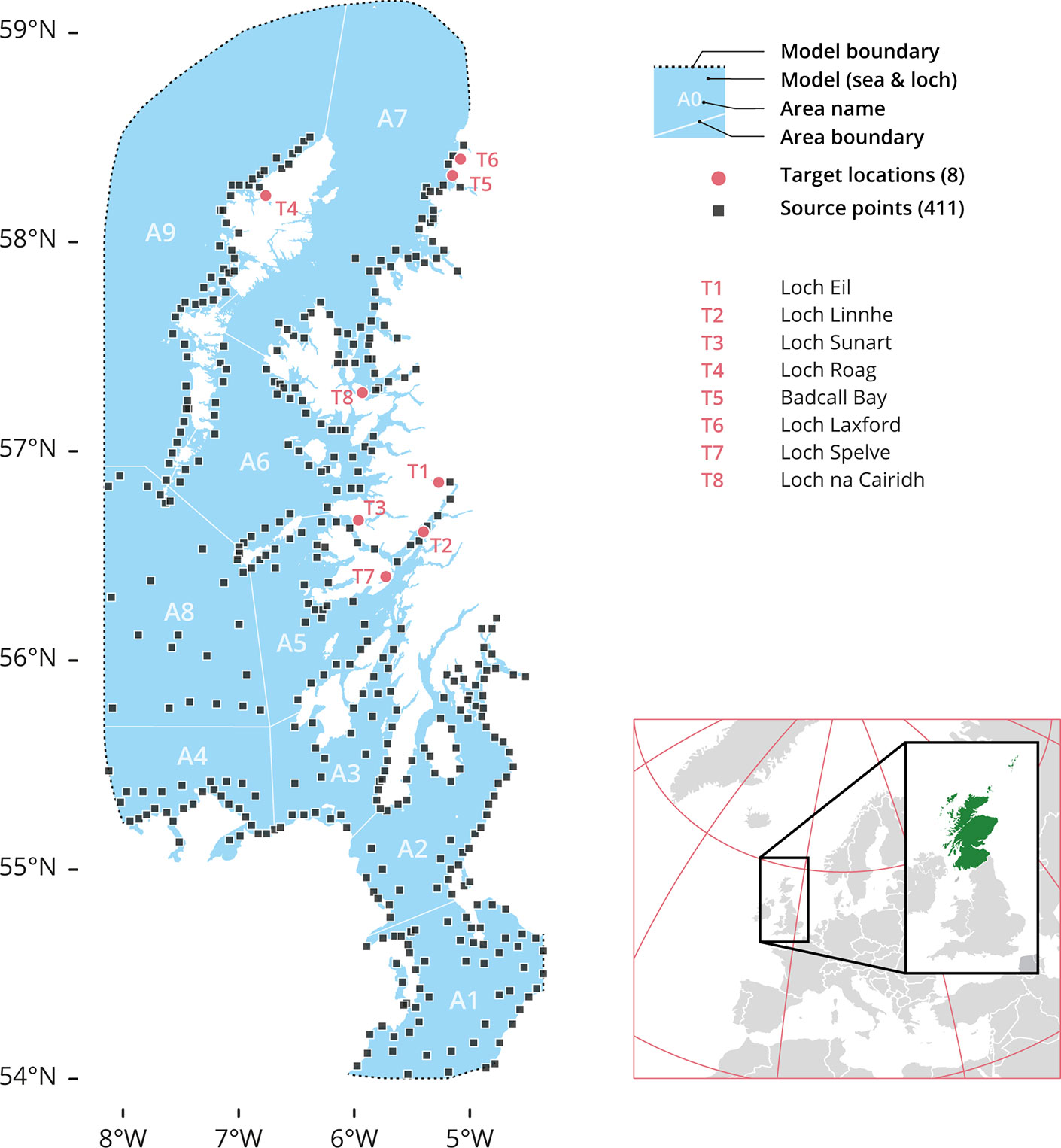
Figure 1 The Model’s source and target locations. A total of 411 source points (black squares) were used and 8 target sites (red dots): T1 Loch Eil, T2 Loch Linnhe, T3 Loch Sunart, T4 Loch Roag, T5 Badcall Bay, T6 Loch Laxford, T7 Loch Spelve and T8 Loch na Cairidh. The model also spliced the region in 9 geographical area divisions: A1. Northern Irish Sea and Solway Firth; A2. North Channel and Firth of Clyde; A3. Sound of Jura; A4. Malin Head or Northern coast of Ireland; A5. Firth of Lorne (and southern part of Inner Hebrides Sea); A6. South Minch and Small Isles; A7. North Minch; A8. Atlantic and South Hebrides; and A9. West Outer Hebrides.

Biophysical model

The biophysical model was comprised of a hydrodynamic model, a particle tracking model, and a post-processing module to determine the source location of the bivalve larvae. The post-process of data has been made using MATLAB R.2019b. The count of accumulated particles in each area and subsequent count of particles in each target location has been made with the inpolygon function. The data used (Supplementary Table S1) for the ANOVA test is the obtained after counting the accumulation of particles and the statistical test has been done using the anovan function. Finally, the representation of physical variables such as wind roses and current velocity has been done using the WindRose and the cquiver functions, respectively.

Hydrodynamic model

This study’s hydrodynamic model was based on the Finite Volume Coastal Ocean Model (FVCOM; Chen et al., 2006). The WeStCOMS v1 model domain (Aleynik et al., 2016) was expanded in v2 and became operational in April 2019 for hindcast/forecast use (Davidson et al., 2021). Triangular elements in WeStCOMS-FVCOM allowed for variation in element size and were capable of resolving the flow along the complex coastline and bathymetry in fjordic coastal environments such as the West coast of Scotland. The open lateral boundaries of the model were forced (nested) with the output of a high resolution (2 km regular grid) North-East Atlantic ROMS operational model (Dabrowski et al., 2016) supplied by the Marine Institute, Ireland. The layer depths were determined using the uneven terrain-following sigma layer proportions. Tides at the boundaries were calculated using the inverse barotropic tidal solution developed by Oregon State University (Egbert and Erofeeva, 2002). Fresh-water discharge estimates based on precipitation over 228 river catchment basins, as well as fluxes across the air-sea-surface interface, were derived from the regional implementation of Weather Research Forecasting (WRF v4; Skamarock and Klemp, 2008) and run at SAMS. Integration stability of 2D (external) and 3D (internal) momentum equations in mod-splitting hydrostatic FVCOM model is predetermined by the smallest horizontal length-scales (up to 80 m near-shore) and short external time-step 0.3 seconds. Wetting and drying scheme was activated, however, to prevent ‘drying’ all the shoreline nodes assigned fixed value -5 m, assuming that the width of littoral (intertidal zone) along the western Scottish coasts is usually shorter than the nearest model element side. WeStCOMS-FVCOM outputs contain one-hourly snapshots of 3D temperature, salinity, velocity and turbulence fields as well as its surface meteo-forcing 2D time-series. Initial WeStCOMS (v1) simulations cover the period between June 2013 and June 2019 and switched to extended domain (v2) since April 2019 to run operationally onward. Surface elevation, velocity, temperature, salinity, and turbulence intensity were among the model outputs. The hydrodynamic model’s accuracy had been tested using multiple oceanic observations (Aleynik et al., 2016; Davidson et al., 2021). The International Hydrographic Office provided the sites data for tidal analyses and comparison. Temperature, salinity, and current data were obtained from conductivity, temperature and depth (CTD) transects and thermistor loggers (Inall et al., 2009), as well as an 18-year time series of currents and subsurface CTD readings (Fehling et al., 2006) and recently deployed several sea-gliders missions in south-western model segment. Comprehensive description of the model’s skills validation against observational data near shore was given in (Aleynik et al., 2016) and recently published (Davidson et al., 2021).

The hydro-files containing weather data implemented for WeStCOMS-FVCOM can be found at https://thredds.sams.ac.uk/thredds/catalog/scoats-westcoms2/catalog.html (folders covering 2017 to 2021).

Particle tracking model

Particle tracking was conducted using the model of Adams et al. (2014; 2016). This was originally developed to predict dispersal and linked physical processes such as water movements with biological processes such as maturation and mortality. The movement of larvae incorporated advection due to local currents and horizontal diffusion equal to 0.1 m² s^-1. Particle depths below the water surface were fixed for the duration of each simulation (meaning trajectories were effectively 2D). Particle movement vectors were set to zero when they would have taken the particle onto land.

Maturation and mortality were omitted from the particle definition, however we made use of a ‘settlement window’ for the ‘tidal release’ simulations. Details relating to particle numbers, source sites and release schedule are given in the subsections ‘Single day release simulations’ and ‘Tidal cycle release simulations’.

Velocities at particle locations were interpolated horizontally and vertically from WeStCOMS-FVCOM irregularly grid current output, and the model is integrated using a fourth-order Runge Kutta scheme.

The particle tracking code can be found at https://github.com/tomadams1982/BioTracker (commit 9fbf1bb). The software used to run the particle tracking model was NetBeans v11.3i, an integrated development environment for Java.

Post process

The domain area (West coast of Scotland) was partitioned into 9 different geographical areas (Figure 1) for reporting analysis purposes (A1 to A9). Each geographical area had several source points from which the larvae were released during the simulations. Finally, within the domain area, 8 aquaculture sites with bivalve recruitment operations were chosen as target locations for larval settlement (T1 to T8).

Boundaries between A1 and A9 reflected island chains and other natural geographical features, and as such are consistent with the complicated coastlines and flow patterns of the studied area. The following polygons were used to fill the different geographical areas (Figure 1): A1, The Northern Irish Sea and the Solway Firth. A2, The North Channel and the Firth of Clyde. A3, The Sound of Jura. A4, Malin Head to Ireland’s Northern Coast. A5, The Firth of Lorne (including the southern half of the Inner Hebrides Sea). A6, The South Minch and Small Isles. A7, The North Minch. A8, The Atlantic and South Hebrides. And A9, The West Outer Hebrides. The division of the areas help us to identify the release-source coordinates for the particle simulation.

Settlement sites (‘target locations’) included: Loch Eil (T1; Latitude 56.85°N, Longitude 5.27°W), Loch Linnhe (T2; 56.61°N, 5.40°W), Loch Sunart (T4; 56.67°N, 5.96°W), Loch Roag (T4; 58.22°N, 6.77°W), Badcall Bay (T5; 58.31°N, 5.15°W), Loch Laxford (T6; 58.40°N, 5.08°W), Loch Spelve (T7; 56.40°N, 5.73°W) and Loch na Cairidh (T8; 57.28°N, 5.93°W).

Single day release simulations

Single-day release simulations were run to evaluate the particles’ circulation through the mesh from emitter point (‘source points’). We assumed that all bivalves from each source point spawned at the same time, representing a mass-spawning events, which are common in the spring, rather than trickle spawning events, which are more common later in the season (Fernández et al., 2015).

A range of particle tracking simulations were carried out in order to assess variability in predicted dispersal patterns. Like most benthic organisms, bivalves spend their early life stage within the water column, which lasts from three to four weeks (Bayne, 1965; Pineda et al., 2007). We adjusted the simulation start time (1^st March, 1^st April, 1^st May), the release year (2017-2021), dispersal period (30 or 45 days; Helm et al., 2004; Pineda et al., 2007; Demmer et al., 2022), and the particle depth (2 m, 6 m or 10 m below sea level) following literature that indicates mussel pediveliger larvae are found primarily in near-surface waters (Baker and Mann, 2008; Demmer et al., 2022). The total number of released particles was 8,877,600 (20 particles 411 number of sites 24 first hours 3 different months 5 years 3 depths).

On average, the ocean currents around Scotland flow in a clockwise direction along the coast (De Dominicis et al., 2018). Since the water flow within the study region has a dominant northward movement and considering our target locations, we limited the possible source points to areas A1 to A6. During the first 24 hours of each simulation, twenty particles were released per hour from each source points in each region, at a given depth, month, and year. This initial test enabled us to validate the model and to a broad identification of the larvae trajectory and proximity to the selected target locations.

Tidal cycle release simulations

Tidal cycle release simulations were run to determine the source points seeding receiver zones (‘target locations’). After a broad scale identification of the larvae trajectory, we pursued a more realistic scenario releasing particles continuously for the first 14 days to cover a spring/neap cycle. The following simulations were run from 1^st April to 17^th June 2021. Ten particles were released each hour for the first 14 days from the source points located in A1 to A9 at6 m below the sea level (total number of release particles was 6,904,800). For each particle, the coordinates for each release point (source point), settlement site (target location) and arrival time in hours were recorded.

We established a 20 km 20 km square centred on each target site to aggregate particles ending up in proximity to each target location and its surroundings, counting particles moving within these zones during the last 7 days of our period of interest (27^th April to 3^rd May 2021). Each particle had a unique ID and coordinate, making it possible to locate their initial release coordinate (source point). Particle dispersal accumulation has been converted into density values by dividing particle counts within mesh elements by the element area (particles/m³).

Results

Physical variables affecting the simulation of particles

Using April 2021 as an example, the wind rose (Figure 2A) shows that winds from the North-West sector occur 10% of the time, reaching maximum speeds of 9.6 m/s to 11.0 m/s from those directions. The same is happening from the south, but in this case, winds reach speeds between 7.3 m/s and 9.6 m/s. There is a general wind flow occurring from the North-West. In April 2020 (Supplementary Figure S1), the wind rose shows that winds from the east sector occur 9% of the time, reaching maximum speeds of 3.0 m/s to 6.0 m/s. However, the greatest speed is coming from the south sector just 2% of the time, achieving maximum speeds of 12.0 m/s to 15.0 m/s.

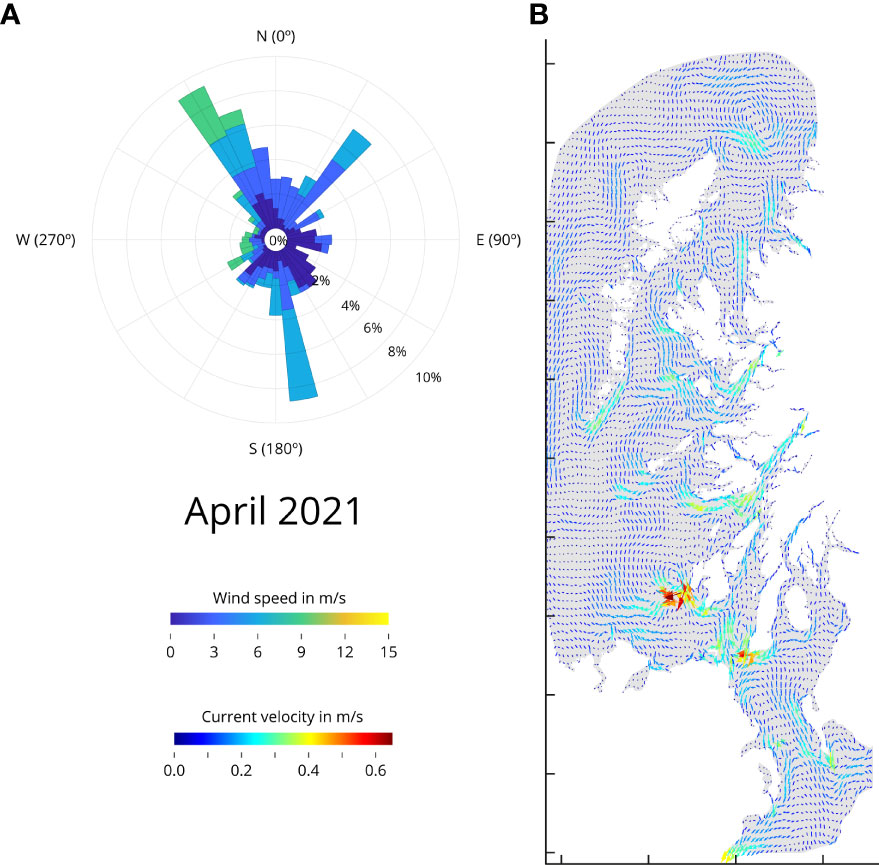
Figure 2 Wind rose and surface current velocity for April 2021. (A) Wind rose. The wind direction determined by where it blows to. The color scale represents wind speed (m/s), whereas the inner circle represents frequency. The data are from WRF v4. (B) Average current velocity between 0 m to 10 m below sea level (m/s). Detailed Wind roses and for average surface current velocity for March, April, and May 2021 and 2020 are available Supplementary Figures S1, S2 respectively.

The wind is a major driving force for the currents, and the model allows for the estimation of average current speeds throughout Scotland’s West coast. Sea-surface currents (0 to 10 m below sea level) suggest a mainly northward flow with velocities of 0.3 m/s to 0.4 m/s dominating in the open areas of the basin in March and April 2021 (Figure 2B and Supplementary Figure S2). The average speed for complex areas and narrow channels goes up to 0.65 m/s. May 2021 however remains calmer, reaching only maximum speeds in the south channel. On the other hand, the intense current speeds in March 2020, are not present in April 2020, where the sea surface currents show a calmer picture for that year and month; only in the north, between Western Isles and the Highlands, the sea surface currents reach maximum speeds of 0.5 m/s to 0.6 m/s, and May 2020 remains similar as in year 2021. The combination of wind rose data with the sea surface currents, provides an understanding for the observed variability in determined areas of the West coast of Scotland.

Variability analysis

We carried out a regression analysis to identify significant differences within groups in our data set. Being years, release areas, target areas, and months the nominal variables (factors); depth continuous variable (co-variate), and accumulation of particles (in each settlement area) the continuous dependent variable (Table 1). Results suggest that there is not a noticeable change in overall structure between the depths, years, and months. The only significant differences are between source areas (settlement sites) and target areas (P-value 0.001).

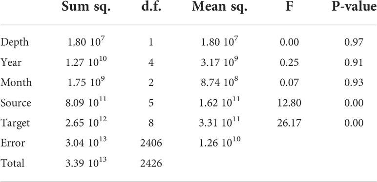
Table 1 Analysis of variance. Sq Square; d.f. degree of freedom.

Single day releases

When combined with the climatic pattern, the particle tracking model yielded large-scale patterns of larval distribution that were consistent with expectations. We compared a 30-day simulation period to a 45-day simulation period, with the first days of the simulations being 1^st March, 1^st April, and 1^st May.

When analyzing the variability between years 2017-2021 (Figure 3) and between depths in one specific year, 2021 (Figure 4), climatic conditions need to be considered to understand the annual differences in the particle dispersion. The identification of physical parameters influencing the larvae trajectory between years has been done, producing wind roses and current surface velocity plots for the years 2020-2021 (Figure 2 and Supplementary Figures S1, S2). In general, annual variability is higher since the weather fluctuations are affecting the overall integrated transport of our fixed-depth particles from one year to another due to the fact that model momentum equations include the wind-driven, the density-driven (baroclinic) and tidal (barotropic) components. When looking at the variability between depths, the retention of our fixed-depth particles remains similar at 2 m, 6 m, and 10 m depth for year 2021.

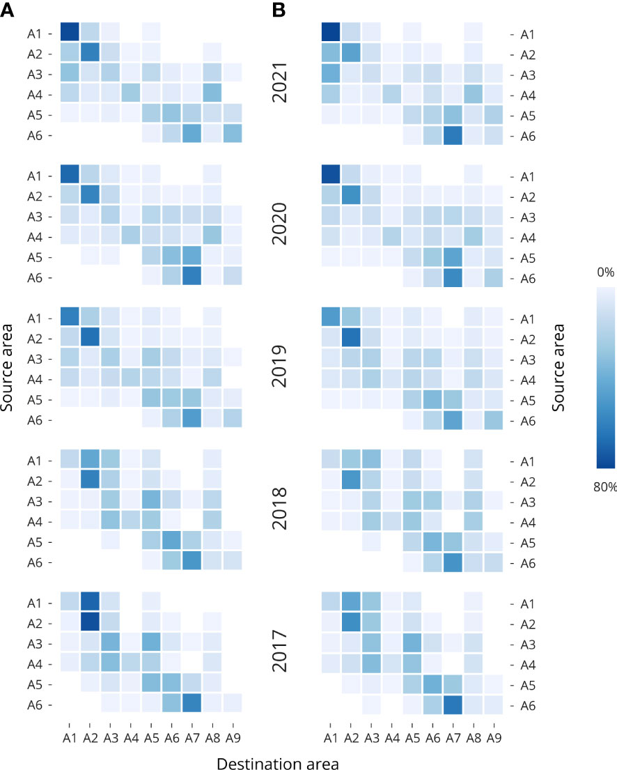
Figure 3 Heatmaps of the particle connectivity between the source (Y axis) and destination area (X axis). The particle accumulations from Single day release setup, where the accumulation for each source regions have been averaged for March, April, and May at 2 m, 6 m, and 10 m depth for the years 2021 to 2017; (A) 30-day release and (B) 45-day release with beginning points on 1^st March, 1^st April, and 1^st May 2021. Dark blue boxes corresponding to areas with higher particle accumulation and light blue to white boxes corresponding to areas with lower particle accumulation in percent. Detailed means and standard deviations are provided in Supplementary Table S2.

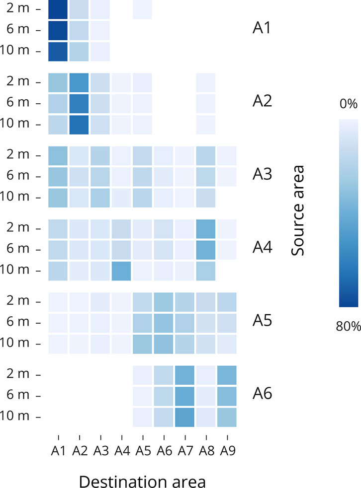
Figure 4 Heatmaps showing particle connectivity between the source (Y axis) and destination (X axis) areas for the Single day set up. For the years 2021, the accumulation for each source region was averaged for March, April, and May at each depth. Dark blue boxes represent area with high particle accumulation, whereas light blue to white boxes represent areas with lower particle accumulation in percent. Supplementary Table S3 has detailed means and standard deviations.

During the 30-day simulation (Figure 3A and Supplementary Table S2), the release of particles from the source points in A1 in years 2021, 2020 and 2019 show higher retention of particles in that same destination area (A1), but more dispersal towards A2 in years 2018 and 2017. With 81.7%, 72.3% and 63% of particles accumulated in A1 for years 2021, 2020, and 2019. The release of particles from source points in A2 show higher retention of particles in all the years. With 15.2% and 15.5% of particles accumulated in A1, and 45.1%, and 72.7% in A2 for years 2019 and 2018. From the release of particles from source points in A3, A4, and A5 the dispersion of particles across the rest of the areas is more predominant in all the years. Finally, the release of particles from the source points in A6 show dispersion of the particles mainly between the areas in A6 (16.1%, 22.1%, 22.1%, 27.1%. And 32.4% for years 2021, 2020, 2019, 2018, and 2017, respectively), and A7 (43.8%, 62.9%, 50.6%, 53.6%, and 61.1%, for years 2021, 2020, 2019, 2018, and 2017, respectively). During the 45-day simulation period (Figure 3B and Supplementary Table S3), the release of particles from the source points in A1 to A6 show a similar pattern as the one described for the 30-day simulation period. But since the particles have been circulating for 45 days, slightly more dispersion has been observed. However, the release of particles from the release points in A1 and A2 keep reflecting higher particle retention values. Details particle dispersal through 2021 for March, April, and May, at 2 m, 6 m and 10 m depth are available in Supplementary Figure S3.

Tidal cycle releases

Through the tidal cycle simulations, we have identified possible source points of larvae for every aquaculture site. After analyzing 5 years of particle dispersal within three different depths, and since our variability analysis (Figure 4) between depths showed not significant changes in the movement of particles for 2021, for our purpose (finding the possible source points of the larvae ending up in our target locations) we decided to focus on April 2021 at 6 m depth. Our results represent a week window, from the 27^th of April to the 3^rd of May (i.e., four weeks of pediveliger larvae swimming through the water body plus three extra days assuming larvae does not settle exactly the 30^th of April). The results are shown in Figure 5 and visually, there is a clear particle dispersal separation between particles released from source points located in southern areas (A1 to A4) compared to the particles released from source points located in the central-northern areas (A5 to A9).

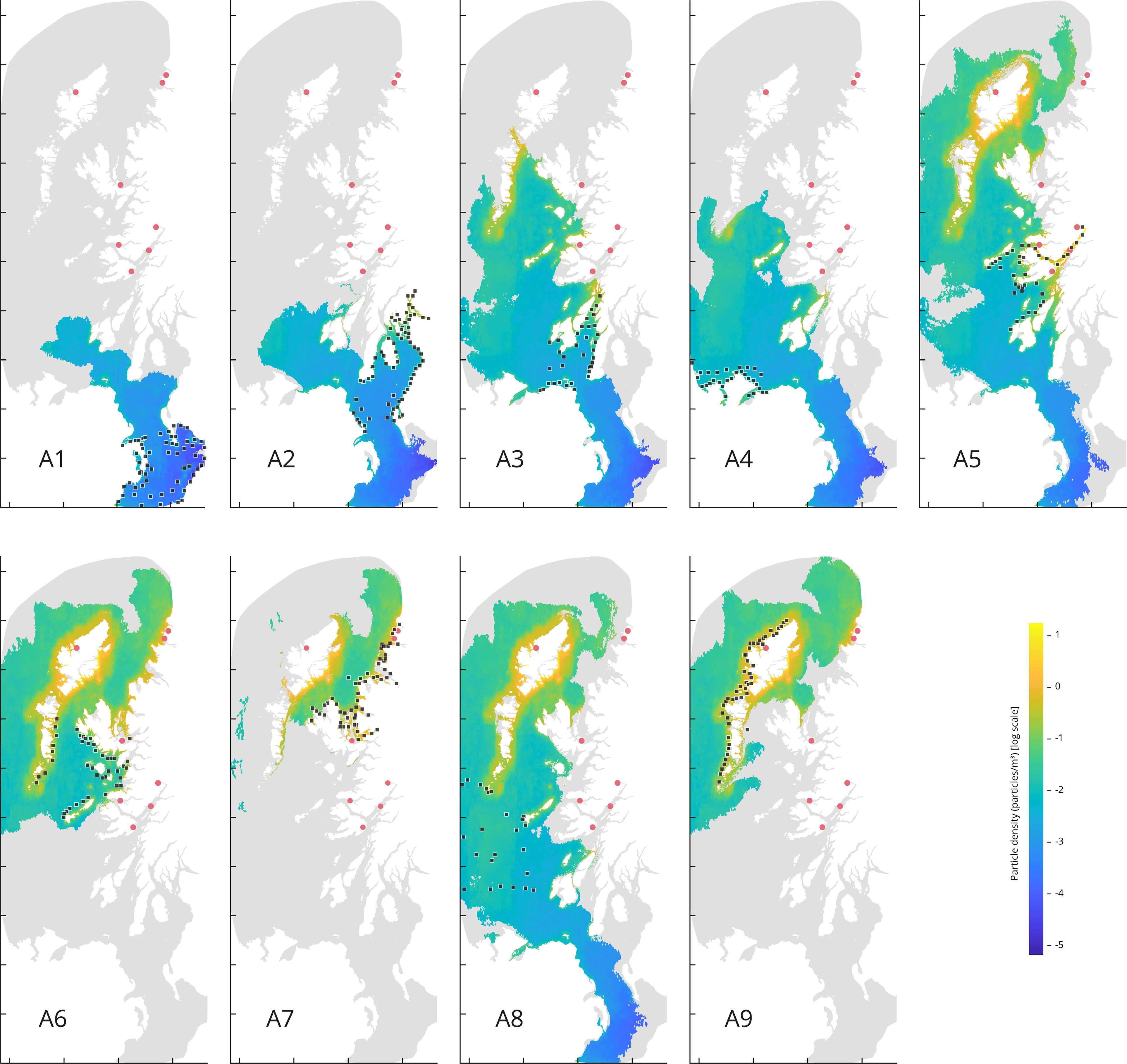
Figure 5 Particle density (particles/m³) from particles released from each source area. the map depicts the period from 27^th April to 3^rd May 2021, at a depth of 6 m. Tidal cycle releases simulation set up (continuous release for the first 14 days). The red dots represent the eight target sites. Each source points from the area A1 through A9 are represented by a black square.

Higher densities values are observed for the releases occurred in source areas corresponding to A5, A6, A7, A8 and A9, with density values of 2.39, 2.70, 3.04, 2.06, and 2.34 particles/m³, respectively. Whilst the lowest mean density values are coming from the source areas corresponding to A1, A2, A3, and A4, with density values of 0.02, 0.12, 0.38 and 0.10 particles/m³, respectively.

Releases from A1 and A2 (Figure 5) show less particle dispersal compared to the rest of the source areas. Although the results for A3 and A4 show more particle dispersal, the maximum density values do not coincide with our target locations. The higher density accumulation sourced from A5 coincides with four of the target locations: Loch Eil, Loch Linnhe, Loch Spelve and Loch Sunart. The higher density accumulation sourced from A6 coincides with the target locations corresponding to Loch na Cairidh, Loch Roag, Badcall Bay, and Loch Laxford. The higher density accumulation sourced from A7 coincides with the target locations corresponding to Badcall Bay, Loch Laxford, and Loch na Cairidh. The higher density accumulation source from A8 coincides with Loch Roag. And lastly, the higher density accumulation source from A9 coincides with Loch Roag, Badcall Bay, and Loch Laxford.

Source location identification

The particles released from each geographical source area on the last day of our period of interest (tidal cycle releases simulation set up, continuous particle release for the first 14 days), 27^th April to 3^rd May 2021at 6 m depth, were quantified in each target location, and found within the 20 km defined area (Table 2). The source point closest to the target location is just 6 km away, and the source point being further away is 170 km far from the target location. For example, all the particles observed in Loch Eil originate from the same place, A5-1 (6 km to the target location). The results suggest (Supplementary Figure S4) that none of the particles emitted from the sources areas A1 to A4 seed any of the target locations, however particles released from A5 appear to seed the majority of our target locations (5/8 target locations). Furthermore, T4 (Loch Roag) is the target location that receives particles from the majority of the source areas (A5, A6, A8, and A9).

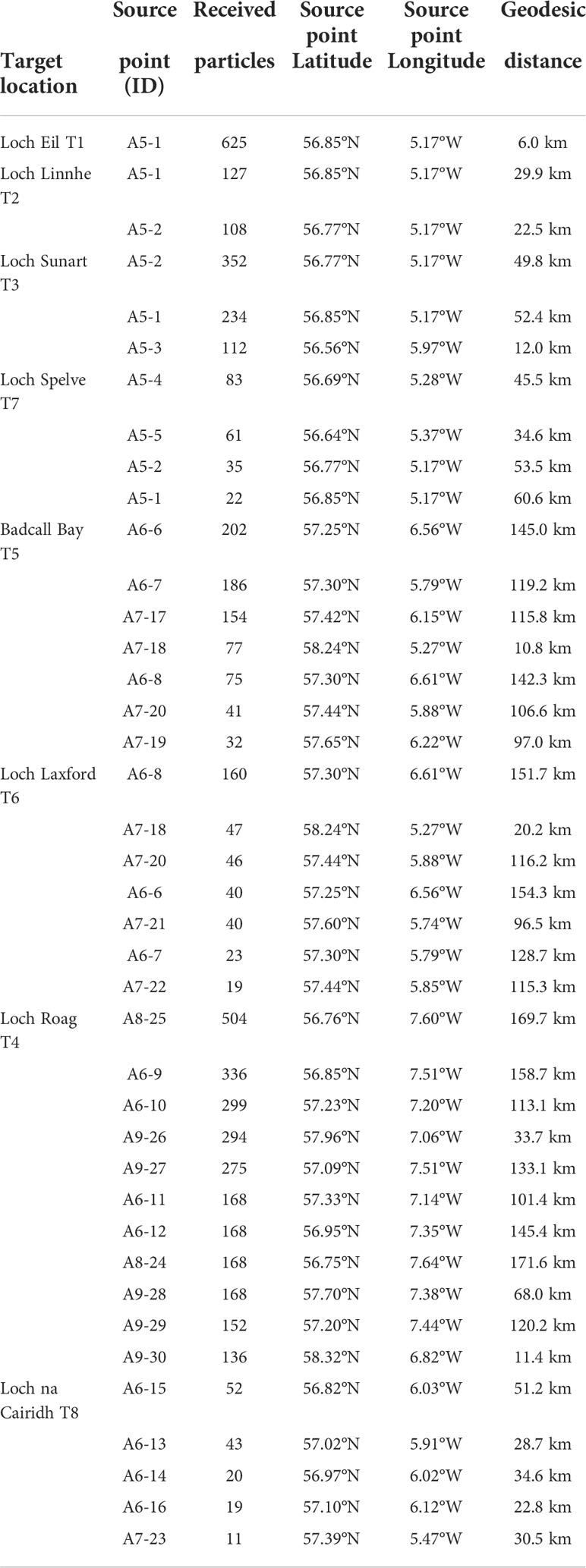
Table 2 Identification of the major source points contributor for each target locations.

Based on the source point locations, we found three types of larval recruitment dynamics: self-recruiting, self-recruiting with external recruitment influence, and low-self-recruitment with high external recruitment influence (Table 2). Figure 6 depicts an example of each case: self-recruiting site, A5-1 is the only source points for the target location in T1 (Figure 6B); self-recruitment with external recruitment influence, A5-1 and A5-2 are the source points for T2 (and Figure 6B) and A5-1, A5-2, and A5-3 are the source points for T7. Finally, Figure 6C depicts an example of low-self-recruitment with high external recruitment influence for T4 where source points are in A6, A8, and A9.

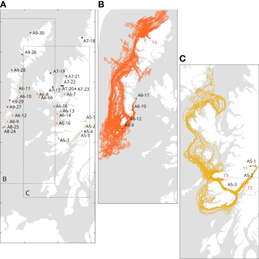
Figure 6 Details of the source locations significantly contributing to the particle accumulations at each target locations. (A) Representation of the source points; (B) Cases of self-recruitment, Loch Eil (T1), and self-recruiting and influence of external recruitment for Loch Linnhe (T2) and Loch Sunart (T3); (C) Example of external recruiting only: Loch Roag (T4). To avoid visual clutter, only the source points A6-9 to A6-12 are illustrated. Distinct colors represent different geographical areas. Details are available in Supplementary Table S4.

Discussion

Inter-annual variability in larval dispersal and connectivity of bivalve populations in the West coast of Scotland has been investigated through the parameterization of a particle tracking model exposed to climatic variables. Our models represent two plausible scenarios: the first (single day releases), confirmed the optimum larval movement through the mesh representing the West coast of Scotland; and the second (tidal cycle releases) allowed for the identification of distinct source points for each target location.

The study of bivalve larvae trajectory in Scotland is still a work in progress, model scenarios were designed following observations made by literature on inter-annual variability of seed recruitment and to a lesser extent from shellfish farmers expertise. As mentioned before, in most marine benthic species the pelagic larval stage is capable of much greater dispersal than juveniles and adults, making the fate of larvae a key determinant of marine population connectivity (Pineda et al., 2007; Cowen and Sponaugle, 2009). Previous studies have shown the importance of circulation patterns on interannual variability of larval recruitment and dispersal (McQuaid and Phillips, 2000; Largier, 2003), and interactions between larval vertical migration and stratification have been shown to be an important driver of dispersal (Raby et al., 1994). Moreover, the water column in the West coast of Scotland remains well mixed since winter until May, which implies that stratification might not play a role in earlier spring on larval dispersal, as also shown in Figure 4; this is in addition supported by Demmer et al. (2022) for the study of mussel dispersion in the northern Irish Sea.

In our model study, virtual larvae distributed at 6 m depth dispersed away from their native bed to a target location by a maximum of 170 km after four weeks, suggesting both local connectivity and general connectivity within the West coast of Scotland. Our results show that there is no significant difference in dispersal patterns between the three depths tested by the model. Indeed, assuming that larvae are distributed throughout the water column, performing only a limited vertical migration and in the absence of stratification, then their dispersal would be primarily controlled by tidal currents (Raby et al., 1994; McQuaid and Phillips, 2000; Demmer et al., 2022). Furthermore, assuming that bivalve larvae are mainly distributed in the near-surface waters, their dispersal would additionally be influenced by wind-driven currents. Currents can be divided into tidal (barotropic) and non-tidal (residual) components. We assumed that residual currents in the higher layers are primarily generated by a combination of two factors: wind stress and pressure variations caused by density gradients. Seasonal thermal vertical stratification is highest in the summer, whereas saline stratification is associated with nearshore sources of freshwater discharge in sea-lochs and along coasts. Larvae released from the Northern Irish Sea and Solway firth (A1); North Channel and Firth of Clyde (A2); Sound of Jura (A3) and Malin Head (A4) present more particles retention and less accumulation after four weeks, meaning that the southern part of the West coast of Scotland is facing a barrier for the larvae to travel northwards. This can be observed in Figure 2B with dynamic velocity currents facing maximum values in the south channel. On the other hand, the larvae released from Firth of Lorne (A5); South Minchand Small Isles (A6); North Minch (A7); Atlantic and South Hebrides (A8); and West Outer Hebrides (A9) all present a higher dispersion of the particles as well as greater particle accumulation after four weeks. This first observation might be important for aquaculture practices; larvae from the southern part of the West coast of Scotland (A1 to A4) might have different genetic structure if compared to the northern part of the West coast of Scotland (A5 to A9).

Looking closely to the source points seeding in T1, T2, T3 and T7, the particles are coming from the same area (A5), being T1 an example of self-recruitment, and T2, T3 (in a lesser extent; Table 2) and T7 receiving seeds from T1. The source points seeding T5 and T6, have their origin in the south and north of Skye peninsula; at the same time, T8 location (north of the Skye peninsula) is in the same area where multiple source points are seeding T5 and T6, suggesting these three target locations might be connected. Finally, the remainder target sites located in A9 (T4) is an example of robust external seed recruitment and to a lesser extent self-recruitment from nearby areas. From A5 to A9 a rapid dispersion of the particles simulating the bivalve larvae is predominant. The fast flow on Scottish waters carrying particles with similar behaviour, e.g., other larvae and sea lice, entail implications for policy and farming practices, disease control and global warming issues.

Even though, we constructed a simulation of particles (bivalve larvae) moving along the West coast of Scotland, our model has significant limitations that will need to be addressed in future studies. For example, the particle tracking model does not account for vertical migration of particles through the different layers of the FVCOM mesh as little data are available to model the phenomenon; no mortality was considered because there is insufficient information on mortality rates for bivalves during the larval phase.

In this study, we show how a biophysical model can help in the understanding of system dynamics and the identification of breeding grounds and settlement areas, which can be utilized to rationalize bivalve farming activities. This biophysical approach could help the understanding of bivalve populations in a dynamic maritime environment such as the West coast of Scotland. Furthermore, our observations on the Scottish waters can help to develop new particle simulations with similar characteristics, e.g., other pelagic larval stages of keystone species and potential pathogens like sea lice. With the corresponding policy, farming, and disease control implications in the face of global warming concerns.

Data availability statement

Publicly available datasets were analyzed in this study. The particle tracking code can be found at https://github.com/tomadams1982/BioTracker (commit 9fbf1bb), while the hydro-files containing weather data implemented for WeStCOMS-FVCOM can be found at https://thredds.sams.ac.uk/thredds/catalog/scoats-westcoms2/catalog.html (folders covering 2017 to 2021).

Author contributions

SC sourced the funding, co-developed the conceptual idea, supervised the findings of this work, and edited the manuscript. TA co-developed the conceptual idea with SC, provided the particle tracking code, trained AC-F to use the particle tracking code, supervised the findings of this work and edited the manuscript. DA Supervised the findings of this work, edited the manuscript, developed and shared the WeStCOMS model output. MB sourced the funding, revised the manuscript and the figures. AC-F sourced and co-developed the conceptual idea with SC and TA, carried out all the particle tracking simulations, conducted all the analysis and wrote the draft of the manuscript. The authors read and approved the final manuscript.

Funding

The NERC SUPER Doctoral Training Program, Fishmongers’ Company, Association of Scottish Shellfish Growers, the Sustainable Aquaculture Innovation Centre, and the University of Stirling funded this work. WeStCOMS hydrodynamic model development and maintenance was supported by the EU’s INTERREG VA and AA Programmes, via ‘Collaborative Oceanography and Monitoring for Protected Areas and Species’ (COMPASS) and ‘Predicting Risk and Impact of Harmful Events on the Aquaculture Sector’ (PRIMROSE) projects, and a several UKRI grants: ‘Combining Autonomous observations and Models for Predicting and Understanding Shelf seas’ (CAMPUS NE/R00675X/1) and ‘Evaluating the Environmental Conditions Required for the Development of Offshore Aquaculture’ (OFF-AQUA, BB/S004246/1). The funding bodies played no role in the design of the study and collection, analysis, and interpretation of data and in writing the manuscript.

Conflict of interest

TA is employed by Scottish Sea Farms Limited.

The remaining authors declare that the research was conducted in the absence of any commercial or financial relationships that could be construed as a potential conflict of interest.

Publisher’s note

All claims expressed in this article are solely those of the authors and do not necessarily represent those of their affiliated organizations, or those of the publisher, the editors and the reviewers. Any product that may be evaluated in this article, or claim that may be made by its manufacturer, is not guaranteed or endorsed by the publisher.

Supplementary material

The Supplementary Material for this article can be found online at: https://www.frontiersin.org/articles/10.3389/fmars.2022.985748/full#supplementary-material

References

Adams T., Aleynik D., Black K. (2016). Temporal variability in sea lice population connectivity and implications for regional management protocols. Aquacult. Environ. Interact. 8, 585–596. doi: 10.3354/aei00203
Adams T. P., Aleynik D., Burrows M. T. (2014). Larval dispersal of intertidal organisms and the influence of coastline geography. Ecography 37, 698–710. doi: 10.1111/j.1600-0587.2013.00259.x
Aleynik D., Dale A. C., Porter M., Davidson K. (2016). A high resolution hydrodynamic model system suitable for novel harmful algal bloom modelling in areas of complex coastline and topography. Harmful Algae 53, 102–117. doi: 10.1016/j.hal.2015.11.012
Baker P., Mann R. (2008). Late stage bivalve larvae in a well-mixed estuary are not inert particles. Estuaries 26, 837–845. doi: 10.1007/BF02803342
Bayne B. L. (1965). Growth and the delay of metamorphosis of the larvae of Mytilusedulis (l.). Ophelia 2, 1–47. doi: 10.1080/00785326.1965.10409596
Chen C., Beardsley R. C., Cowles G. (2006). An unstructured grid, finite-volume coastal ocean model (FVCOM) system. Oceanography 19, 78–19. doi: 10.5670/oceanog.2006.92
Clark S., Hubbard K. A., McGillicuddy D. J., Ralston D. K., Shankar S. (2021). Investigating Pseudo-nitzschia australis introduction to the gulf of Maine with observations and models. Continental Shelf Res. 228, 104493. doi: 10.1016/j.csr.2021.104493
Cowen R. K., Sponaugle S. (2009). Larval dispersal and marine population connectivity. Annu. Rev. Mar. Sci. 1, 443–466. doi: 10.1146/annurev.marine.010908.163757
Dabrowski T., Lyons K., Nolan G., Berry A., Cusack C., Silke J. (2016). Harmful algal bloom forecast system for SW ireland. part I: Description and validation of an operational forecasting model. Harmful Algae 53, 64–76. doi: 10.1016/j.hal.2015.11.015
Davidson K., Whyte C., Aleynik D., Dale A., Gontarek S., Kurekin A. A., et al. (2021). HABreports: Online early warning of harmful algal and biotoxin risk for the Scottish shellfish and finfish aquaculture industries. Front. Mar. Sci. 8. doi: 10.3389/fmars.2021.631732
De Dominicis M., Wolf J., O’Hara Murray R. (2018). Comparative effects of climate change and tidal stream energy extraction in a shelf sea. J. Geophysical Research: Oceans 123, 5041–5067. doi: 10.1029/2018JC013832
Demmer J., Robins P., Malham S., Lewis M., Owen A., Jones T., et al. (2022). The role of wind in controlling the connectivity of blue mussels (Mytilus edulis l.) populations. Movement Ecol. 10, 3. doi: 10.1186/s40462-022-00301-0
Egbert G. D., Erofeeva S. Y. (2002). Efficient inverse modeling of barotropic ocean tides. J. Atmospheric Oceanic Technol. 19, 183–204. doi: 10.1175/1520-0426(2002)019<0183:EIMOBO>2.0.CO;2
Fehling J., Davidson K., Bolch C., Tett P. (2006). Seasonality of Pseudo-nitzschia spp. (Bacillariophyceae) in western Scottish waters. Mar. Ecol. Prog. Ser. 323, 91–105. doi: 10.3354/meps323091
Fernández A., Grienke U., Soler-Vila A., Guihéneuf F., Stengel D. B., Tasdemir D. (2015). Seasonal and geographical variations in the biochemical composition of the blue mussel (Mytilus edulis l.) from Ireland. Food Chem. 177, 43–52. doi: 10.1016/j.foodchem.2014.12.062
Gawarkiewicz G., Monismith S., Largier J. (2007). Observing larval transport processes affecting population connectivity: Progress and challenges. Oceanography 20, 40–53. doi: 10.5670/oceanog.2007.28gawarkiewicz2007
Gosling E. (2003). “Ecology of bivalves”. in Bivalve Molluscs (Oxford, UK: Blackwell publishing Ltd), 44–86.
Hellberg M. E. (2009). Gene flow and isolation among populations of marine animals. Annu. Rev. Ecol Evol Systematics 40, 291–310. doi: 10.1146/annurev.ecolsys.110308.120223
Helm M. M., Bourne N., Lovatelli A. (2004). Hatchery culture of bivalves: A practical manual. no. 471 in FAO fisheries technical paper (Rome, Italy: Food and agriculture organization of the united nations).
Inall M., Gillibrand P., Griffiths C., MacDougal N., Blackwell K. (2009). On the oceanographic variability of the north-West European shelf to the West of Scotland. J. Mar. Syst. 77, 210–226. doi: 10.1016/j.jmarsys.2007.12.012
Jahnke M., Jonsson P. R. (2022). Biophysical models of dispersal contribute to seascape genetic analyses. Philos. Trans. R. Soc. B: Biol. Sci. 377, 20210024. doi: 10.1098/rstb.2021.0024
Largier J. L. (2003). Considerations in estimating larval dispersal distances from oceanographic data. Ecol. Appl. 13, 71–89. doi: 10.1890/1051-0761(2003)013[0071:CIELDD]2.0.CO;2
McQuaid C., Phillips T. (2000). Limited wind-driven dispersal of intertidal mussel larvae: in situ evidence from the plankton and the spread of the invasive species Mytilus galloprovincialis in south Africa. Mar. Ecol. Prog. Ser. 201, 211–220. doi: 10.3354/meps201211
Pineda J., Hare J., Sponaugle S. (2007). Larval transport and dispersal in the coastal ocean and consequences for population connectivity. Oceanography 20, 22–39. doi: 10.5670/oceanog.2007.27
Raby D., Lagadeuc Y., Dodson J. J., Mingelbier M. (1994). Relationship between feeding and vertical distribution of bivalve larvae in stratified and mixed waters. Mar. Ecol. Prog. Ser. 103, 275–284. doi: 10.3354/meps103275
Shanks A. L. (2009). Pelagic larval duration and dispersal distance revisited. Biol. Bull. 216, 373–385. doi: 10.1086/BBLv216n3p373
Skamarock W. C., Klemp J. B. (2008). And forecasting applications. J. Comput. Phys. 227, 3465–3485. doi: 10.1016/j.jcp.2007.01.037
Smaal A. (2002). European Mussel cultivation along the Atlantic coast: Production status, problems and perspectives. Hydrobiologia 484, 89–98. doi: 10.1023/A:1021352904712
Weersing K., Toonen R. (2009). Population genetics, larval dispersal, and connectivity in marine systems. Mar. Ecol. Prog. Ser. 393, 1–12. doi: 10.3354/meps08287
Widdows J. (1991). Physiological ecology of mussel larvae. Aquaculture 94, 147–163. doi: 10.1016/0044-8486(91)90115-N
Wijsman J. W. M., Troost K., Fang J., Roncarati A. (2019). Global production of marine bivalves. Trends and challenges. Goods and Services of Marine Bivalves. Eds. Smaal A. C., Ferreira J. G., Grant J., Petersen J. K., Strand Ø. (Cham, Denmark: Springer International Publishing), 7–26. doi: 10.1007/978-3-319-96776-9_2
Willis J. (2011). Modelling swimming aquatic animals in hydrodynamic models. Ecol. Model. 222, 3869–3887. doi: 10.1016/j.ecolmodel.2011.10.004
Keywords: bivalve, larval dispersal, particle tracking, Scotland, Aquaculture, finite volume coastal ocean model
Citation: Corrochano-Fraile A, Adams TP, Aleynik D, Bekaert M and Carboni S (2022) Predictive biophysical models of bivalve larvae dispersal in Scotland. Front. Mar. Sci. 9:985748. doi: 10.3389/fmars.2022.985748
Received: 04 July 2022; Accepted: 17 August 2022;
Published: 12 September 2022.
Edited by:
Lorenzo Mari, Politecnico di Milano, ItalyReviewed by:
Peter Robins, Bangor University, United KingdomJonathan Demmer, Bangor University, United Kingdom
Copyright © 2022 Corrochano-Fraile, Adams, Aleynik, Bekaert and Carboni. This is an open-access article distributed under the terms of the Creative Commons Attribution License (CC BY). The use, distribution or reproduction in other forums is permitted, provided the original author(s) and the copyright owner(s) are credited and that the original publication in this journal is cited, in accordance with accepted academic practice. No use, distribution or reproduction is permitted which does not comply with these terms.
*Correspondence: Michaël Bekaert, michael.bekaert@stir.ac.uk