SN 2022jli: A Type Ic Supernova with Periodic Modulation of Its Light Curve and an Unusually Long Rise

We compute a pseudobolometric light curve by integrating under the BgcVrGoiz-band observations using the publicly available code SUPERBOL (Nicholl 2018). From our bolometric light curve we measure a peak luminosity L_opt = 10^42.08±0.04 erg s⁻¹, which is within the typical range of SESNe found by Prentice et al. (2019). The total integrated luminosity (across the wavelength range covered by our filters) is E_opt ≈ 2.5 × 10⁴⁹ ergs.

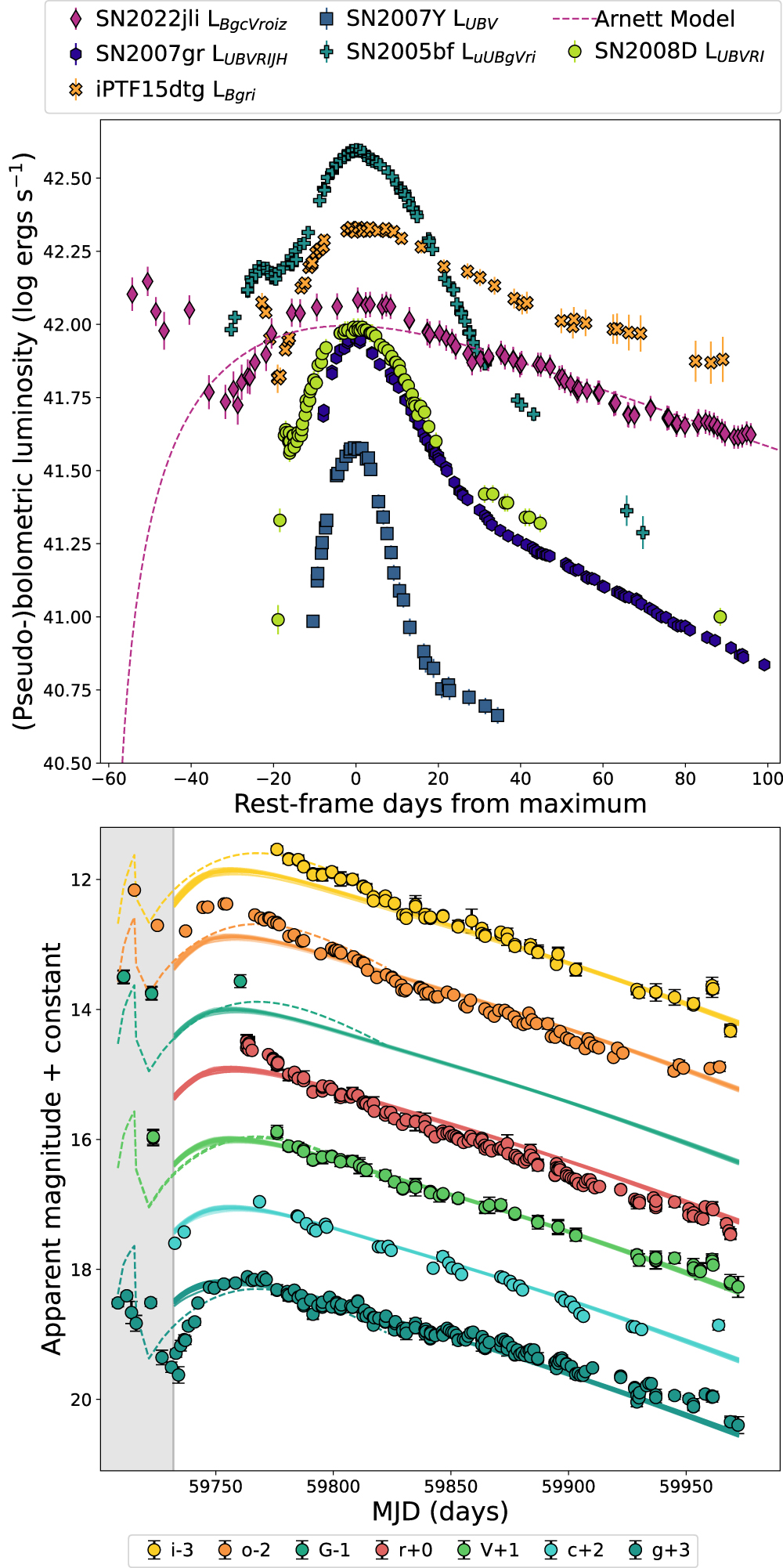
We compare the (pseudo)bolometric light curve to other SNe, including normal SESNe and those with double-peaked light curves, in Figure 3. SN 2022jli exceeds the peak brightness of the Type Ic SN 2007gr (Hunter et al. 2009), the Type Ib SN 2008D (Soderberg et al. 2008; Modjaz et al. 2009), and the relatively faint Type Ib SN 2007Y (Stritzinger et al. 2009), showing a significantly more luminous broad peak and slower decay. SN 2007gr and SN 2007Y both display a monotonic rise and smooth decline, typical of a normal Type Ibc SN, unlike the double-peaked structured light curve of SN 2022jli. The overall shape of the light curve resembles the unusual Type Ic iPTF15dtg (Taddia et al. 2016). Both SNe have a fast-declining early excess with a broad persistent maximum. SN 2005bf (Anupama et al. 2005) has an early peak and broad maximum but is significantly more luminous than SN 2022jli and declines significantly faster.

Zoom In Zoom Out Reset image size

We model the light curve using simple models to derive a representative ejecta mass estimate for SN 2022jli using the Modular Open Source Fitter for Transients (MOSFiT; Guillochon et al. 2018). MOSFiT is a publicly available code that we use to fit semianalytic models to the multiband observed light curves of SN 2022jli. We use two models, one where we model only the broad "main" peak assuming radioactive decay of ⁵⁶Ni as the only energy source (Arnett 1982; Nadyozhin 1994), and another where we fit the full light curve interpreting the initial excess as shock cooling emission (SCE) from interaction with a CSM and a subsequent radioactively powered "main" peak (Chatzopoulos et al. 2013). All model fitting was performed using the dynamic nested sampler DYNESTY package (Speagle 2020) option in MOSFiT.

The bottom panel of Figure 3 shows the ⁵⁶Ni-only model fit to SN 2022jli. To construct this model, we used the nickel-driven explosion model built into MOSFiT (Nadyozhin 1994), omitting any data during the early excess (before MJD 59732). We modify the priors of the model to require the explosion time to be before discovery, i.e., MJD_explosion < MJD_discovery. The opacity was fixed at κ = 0.1 cm² g⁻¹ and κ_γ = 0.027 cm² g⁻¹. With no prior on ejecta velocity, the data require v_ej ≈ 2500 km s⁻¹ and M_ej ≈ 4 M_⊙; this velocity is much lower than the measurements of the Fe ii lines in the spectra (see Section 4.3). The posterior distribution for this fit is included in the Appendix (Figure 5).

This model reproduces the maximum luminosity for the g and c bands but fits poorly to the redder bands, underestimating the flux particularly in the o and i bands. This simple model also fails to reproduce the fast g-band rise after the light-curve dip and the o-band peak luminosity. Color differences between the model light curve and the observed data are likely due to the blackbody assumption made by MOSFiT, as the true spectrum is dominated by strong emission and absorption lines by the time of maximum light. Further detailed modeling is warranted using more sophisticated techniques, which is beyond the scope of this work. For comparison, we perform an additional Arnett model (Arnett 1982) fit to the bolometric light curve with a χ² fitting approach. Fixing κ = 0.1 cm² g⁻¹ and v_ej ≈ 3000 km s⁻¹, we require M_ej ≈ 6 M_⊙, which is in agreement with the results from MOSFiT. This fit is included in Figure 3.

To gauge the systematic modeling uncertainties within MOSFiT, we run the same nickel-driven model for the main peak with a range of v_ej to determine a probable range of M_ej. A fixed ejecta velocity of v_ej = 3500 km s⁻¹ requires M_ej ≈ 7 M_⊙, v_ej = 6000 km s⁻¹ requires M_ej ≈ 18 M_⊙, and v_ej = 7000 km s⁻¹ forces M_ej ≈ 21 M_⊙. With no pre-explosion nondetections available to constrain the explosion time and large systematic errors on the model, we adopt an indicative mass range for SN 2022jli of M_ej ≈ 12 ± 6 M_⊙.

In the second scenario we consider the contribution of SCE following shock breakout of the ejecta through a dense CSM using the ⁵⁶Ni + CSM (CSMNI) model (Chatzopoulos 2013; Villar et al. 2017; Jiang et al. 2020). SCE is a natural interpretation for a fast-declining excess shortly after explosion and is now regularly detected for a range of SN subtypes. The same assumptions are made for the opacities as before, but the explosion time is left as a free parameter of the fit. We modify the code so that the interaction begins when the ejected material reaches the inner radius of the CSM at R₀. Our results indicate a CSM radius R₀ ∼ 1 au, M_ej ∼ 20 M_⊙, M_CSM ∼ 26 M_⊙, and f_Ni ∼ 0.01 for the early excess to be powered by CSM interaction. Our model (fit to the first 110 days) results in a poor match to the observed data, particularly the colors of the early excess, and requires physically improbable parameters; this model is shown in Figure 3.

Although the Chatzopoulos et al. (2013) model implemented in MOSFiT is relatively simple, the very large ejecta masses required imply that this scenario is physically unlikely. We return to this point in Section 5.2. We also emphasize that there is no robust measurement of explosion time to constrain the model since the earliest epoch from the Monard observations is after the SN appeared from solar conjunction.

A long rise time (exceeding 30 days) is a rare occurrence for Type Ibc SNe (Lyman et al. 2016): long-duration light curves with rise times similar to SN 2022jli arise from only ∼6%–10% of SNe Ibc in a bias-corrected sample (Karamehmetoglu et al. 2023). We estimate that M_ej = 12 ± 6 M_⊙ is required to provide the long rise to maximum light. An ejecta mass this extreme is rare and points to a high-mass progenitor star.

The bumps we observe in the light curve could be due to ejecta interacting with concentric shells of circumstellar material. During the undulation, SN 2022jli is overluminous by ∼1 × 10⁴⁰ erg s⁻¹ for 12.5 days. Using the scaling relation $L=\tfrac{1}{2}{M}_{\mathrm{CSM}}{v}^{2}/{t}_{\mathrm{rise}}$ (Smith & McCray 2007; Quimby et al. 2007; Nicholl et al. 2016), we estimate the mass required for each bump to be M_CSM,bump ≈ 10⁻⁵ M_⊙, assuming v = 7000 km s⁻¹ from Fe ii line velocity measurements, and t_rise = 6.3 days.

The average pre-explosion mass-loss rate needed to produce this CSM mass per undulation can be calculated by setting $\dot{M}/{v}_{w}={M}_{\mathrm{CSM},\mathrm{bump}}/{\rm{\Delta }}R$, where v _w is the wind velocity and ΔR = vt_bump is the radial distance bounding this CSM mass. For an SN velocity v = 7000 km s⁻¹ and t_bump = 12.5 days, this gives $\dot{M}\approx \mathrm{few}\times {10}^{-5}({v}_{w}/1000\,\mathrm{km}\,{{\rm{s}}}^{-1})$ M_⊙ yr⁻¹. This is consistent with the mass-loss rates observed from Wolf−Rayet stars (e.g., Sander & Vink 2020), suggesting that a "typical" wind mass-loss rate could potentially provide the CSM structure needed to explain the periodic undulations of SN 2022jli, if subjected to a periodic modulation.

Nested shells of dust caused by colliding winds in a massive binary system have recently been spectacularly revealed in JWST imaging (Lau et al. 2022). They showed that the 17 observed shells were due to repeated dust formation episodes every 7.93 yr modulated by periastron passage of the companion O5.5fc star in the mutual orbit around the WC7 Wolf−Rayet star. An ejection velocity of v = 7000 km s⁻¹ means that the SN shock front travels Δr ≃ 54 au in 12.5 days. By comparison, the nested dust shells around WR 140 are Δr = 4380 ± 120 au. If SN 2022jli undulations were due to peaks in CSM density similar to WR 140 shells, a binary progenitor would need to eject these shells on timescales ∼100 times more frequent, or with a ∼0.2 yr periodicity. We note that the dust emission in the shells in WR 140 does not necessarily imply enhanced gas densities (Pollock et al. 2021).

In this scenario of concentric shells or rings, one might expect that light-travel time effects could broaden the undulation timescale as the shock expands. As the SN ejecta hits the back and front of the shells at the same time, the light-travel time from the back to front increases as ${\rm{\Delta }}{t}_{\mathrm{lt}}\simeq 2{v}_{\mathrm{ej}}{t}_{\exp }/c$, or about 9 days (after 200 days of expansion). While there will be an integrated signal from all parts of the shell, the effect should be to broaden the timescale of the undulations; should the ejecta be photospheric, the broadening effect will be less. The data do not clearly support such broadening.

We can explore potential progenitor candidates using the BPASSv2.2.2 predictions (Eldridge et al. 2017; Stanway & Eldridge 2018), restricting our search to Type Ic progenitors (see Stevance & Eldridge 2021): we select hydrogen-deficient systems with surface mass hydrogen <0.0001 M_⊙ and surface hydrogen mass fraction <0.01. We also restrict our search to helium-depleted SN progenitors, with helium mass fraction <0.3. We then look for systems that satisfy the period estimate of a WR 140−like scenario by searching for P = 0.07±0.015 yr (the error is chosen to give a window of roughly +/−5 days). Finally, we also impose a luminosity and temperature constraint ($\mathrm{log}(L/{L}_{\odot })\gt 5$ and $\mathrm{log}(T/{T}_{\odot })\gt 4.3$), as we are looking for WR+O star systems. We find 27 BPASS models at solar metallicity that fulfill these requirements, and including the initial mass function weighting, we would expect about 15 such systems to be formed per 1 million M_⊙. All these systems have primary star (SN progenitor) masses in a rather narrow range of 10−13 M_⊙, while the secondaries range from 24.5 to 60 M_⊙. Although all these predicted systems have stellar winds around 0.8 × 10⁻⁵ M_⊙ yr⁻¹, similar to the estimated requirement to create the CSM as mentioned in Section 5.1.1, a key factor in the periodic modulation is the eccentricity of the system. Stellar evolution models such as BPASS assume circularized orbits, so we cannot assess how many systems would be born with and maintain sufficient eccentricity.

An alternative mechanism to produce light-curve bumps in Type Ibc SNe was suggested by Hirai & Podsiadlowski (2022). After an SESN in a binary system, the newly born neutron star (NS) may receive a kick in the favorable direction of its companion. As a result, the NS may penetrate or skim the surface of the binary companion. They predict that material captured from the companion settles around the NS and that the accretion rate is likely to be super-Eddington. The accretion could result in outflows or jets that add further energy to the SN ejecta and result in additional luminosity. Accretion resulting in jets has been modeled by Hober et al. (2022), which they propose could power bumps in the late-time light curves of SNe. Undulations in the light curves of SLSNe have been detected (Nicholl et al. 2016; Inserra et al. 2017; Gomez et al. 2021; Hosseinzadeh et al. 2022; West et al. 2023), but no repeating signature has been confirmed over multiple cycles.

Hirai & Podsiadlowski (2022) calculate that even if only ∼0.01 M_⊙ is captured by the NS and if only ∼1% of that is accreted, then the energy available would be of order E_acc ∼ M_acc c² ∼ 10⁵⁰ erg, which is comfortably enough to power a few percent of the total integrated SN flux of E_rad ≃ 2.5 × 10⁴⁹ erg. The direct interaction invoked in Hirai & Podsiadlowski (2022) requires a fairly fine-tuned kick direction and velocity. However, a milder interaction as discussed in Hirai et al. (2018) and Ogata et al. (2021) may be sufficient. The companion star is inflated by heating from the SN ejecta−companion interaction, and the inflated part of the envelope may interact with the NS, causing periodic accretion on the timescale of the orbit.

Accretion-powered jets after core collapse also have sufficient energy (Soker 2022; Hober et al. 2022) to power the excess flux observed in the light curve of SN 2022jli, but a modulation process is required. In the Hirai & Podsiadlowski (2022) scenario, the gradual inspiral of the NS into the companion is a pathway for the formation of a Thorne−Żytkow object (TŻO). TŻOs, which are NSs inside an envelope of nondegenerate diffuse material, have been predicted in the literature (Thorne & Zytkow 1975, 1977), but very few real candidates exist (O'Grady et al. 2020). An issue of the Hirai & Podsiadlowski (2022) scenario is that the orbit of the NS will decay rapidly (within ∼5 orbits), making 15 orbital cycles problematic. However, in the inflated companion case, the low-density envelope results in slower orbital decay (Hirai et al. 2018; Ogata et al. 2021).

The accreting compact object model can be thought of as an internal powering source. The energy released must diffuse out through the ejecta on timescales determined by the opacity, density, and radius of the optically thick material. Hosseinzadeh et al. (2022) propose that a central origin is disfavored if the dimensionless depth of the powering source, $\delta \simeq \tfrac{{t}_{\mathrm{bump}}{\rm{\Delta }}{t}_{\mathrm{bump}}}{{t}_{\mathrm{rise}}^{2}}$, is significantly less than unity. With Δt_bump ≃ 12.5 and t_rise ≃ 60, this parameter then ranges between 0.2 and 0.7 for the earliest and latest bumps. This would marginally disfavor a central, internal powering source, although Hosseinzadeh et al. (2022) note that the expression is quite approximate and should only be treated as an order-of-magnitude result.

MOSFiT modeling of the early excess with an interaction-powered model requires M_ej ≈ 12 M_⊙, which is compatible with the mass required for the long rise to maximum light. However, the duration requires significant M_CSM (>3 M_⊙ in or modeling), which is very large for a Type Ic SN and would require an exotic mechanism to drive extreme mass loss shortly before explosion, such as pulsational pair-instability SN ejections (Woosley 2017).

Perhaps the apparent duration of SCE is extended owing to enhanced opacity caused by Thomson scattering in the CSM (Moriya & Maeda 2012), which is eventually overtaken by the forward shock. Finally, the red spectrum during the first peak (Grzegorzek 2022) would appear inconsistent with luminous circumstellar interaction at early times (i.e., with compact CSM).

We cannot exclude CSM interaction as the source of the early excess; to do so would require more data to constrain the excess or more sophisticated modeling of the interaction to determine the viability of this scenario.

Here we consider the emission from the collision of ejecta with the binary companion of SN 2022jli using the model suggested by Kasen (2010). In this scenario the interaction shocks the SN ejecta, dissipating kinetic energy causing bright optical/UV emission. This additional contribution to the observed luminosity exceeds the radioactively powered SN for a short period, resulting in an early excess. We investigate the viability of this model using Equations (22) and (23) from (Kasen 2010) to estimate the luminosity and the collision luminosity timescale (t_c ) where (L_c,iso > L_Ni)

$$\begin{eqnarray}&&{L}_{c,\mathrm{iso}}={10}^{43}{a}_{13}{M}_{c}^{1/4}{v}_{9}^{7/4}{\kappa }_{e}^{-3/4}{t}_{\mathrm{day}}^{-1/2}\mathrm{erg}\ {{\rm{s}}}^{-1},\end{eqnarray} \tag{ 1 }$$

$$\begin{eqnarray}&&{t}_{c}\lt 7.3{a}_{13}^{2/5}{M}_{c}^{1/2}{v}_{9}^{3/10}{\kappa }_{e}^{1/10}{\displaystyle \frac{{\kappa }_{\mathrm{Ni}}}{{\kappa }_{e}}}^{2/5}{M}_{\mathrm{Ni},0.6}^{-2/5},\end{eqnarray} \tag{ 2 }$$

where a₁₃ = a/10¹³ cm (a is the orbital separation), M _c = M/M_Ch is the ejecta mass M in units of the Chandrasekhar mass (M_Ch), v₉ = v _t /10⁹ cm s⁻¹, ${v}_{{\rm{t}}}=6\,\times \,{10}^{8}{\zeta }_{v}{({E}_{51}/{M}_{c})}^{1/2}$ cm s⁻¹ (following Kasen 2010, we adopt ζ_v = 1.69), κ_Ni is the opacity in the ⁵⁶Ni-dominated region, and κ_e is the ejecta opacity outside this region. The time since explosion is given as t_day, M_Ni,0.6 = M_Ni/0.6 M_⊙, E₅₁ = E/10⁵¹ erg s⁻¹, and E is the explosion energy. We adopt an indicative ejecta mass of 12 M_⊙ from MOSFiT modeling in Section 4.1.2 and set κ _e = κ_Ni = 0.1 cm² g⁻¹. We set M_Ni ≈ 0.7 (for f_Ni ≈ 0.06 from MOSFiT) and set v _t = 8500 km s⁻¹ from direct measurement of the −29-day spectrum (during the early excess).

To produce the observed early luminosity on the order of ∼10⁴² erg s⁻¹ and timescale of ∼10 days, we would need to have separation ∼1 au. For these parameters we calculate t _c ≲ 17.5 days and L_c,iso ≈ 8 × 10⁴³ erg s⁻¹ for t _d = 2 days and L_c,iso ≈ 2 × 10⁴² erg s⁻¹ for t _d = 20 days.

With these assumptions for separation and ejecta mass, our observations are compatible with the direct collision of the ejecta with the companion star. It is important to note that this scenario requires a favorable viewing angle; Kasen (2010) predicts that the collision should be visible in only ∼10% of cases and that an orbital separation of ∼1 au at the time of interaction may require the object to be close to pericenter. An important additional qualification of the Kasen (2010) model calculation is the assumption that the companion to the exploding star is filling its Roche lobe, as in a thermonuclear binary star explosion. Therefore, this calculation should be regarded only as an illustrative estimate of the energetics of a companion interaction. The progenitor systems considered in Section 5.1.1 have separations of 0.5 au and upward, which is compatible with the 1 au separation adopted for this calculation, although we note that they are typically not filling their Roche lobe and interacting. Should the excess be powered by companion collision, one might expect to observe late-time Hα emission from the companion and at late times observe a surviving but inflated companion star.