


Abstract
Resonant states (RS), also known as quasi-normal modes, arise in spectral expansions of linear response functions of open systems. Manipulation of these spatially 'divergent' oscillating functions requires a departure from the usual definitions of inner product, normalization and orthogonality typical in the studies of closed systems. A multipolar Gaussian regularization method for RS inner products is introduced in the context of light scattering and shown to provide analytical results for the crucial RS inner product integrals in the problematic region exterior to the scattering system. We detail the applicability of this method to arbitrary scattering geometries while providing semi-analytic benchmark results for spherical scatterers. This formulation is then used to highlight the lack of 'convergence' in directly truncated RS spectral expansions and the necessity of adding non-resonant contributions to the RS spectral expansions. Solutions to these difficulties are illustrated in the case of dispersive media spheres, but these methods should prove generalizable to arbitrary RS spectral expansions.
Export citation and abstract BibTeX RIS

Original content from this work may be used under the terms of the Creative Commons Attribution 4.0 licence. Any further distribution of this work must maintain attribution to the author(s) and the title of the work, journal citation and DOI.
1. Introduction
The eigenstates of open systems, known as resonant states (RSs), can be viewed as a means of simultaneously describing both the spatial and temporal behavior of the oscillatory 'eigenmodes' of an open system. As such, RSs have been a fruitful, albeit problematic, concept in many branches of physics for over a century [1], where they have been given a wide variety of names like: quasi-normal modes, transient modes, and the famous leaky modes of wave-guides. The RS concept was widely developed in quantum mechanics [2] after its pioneering success by Gamow in describing alpha decay [3], and later by Siegert for characterizing nuclear reactions [4]. Throughout the 20th century, quantum RS descriptions continued to draw the attention of prominent physicists like Wigner [5], Peierls [6], and Zel'dovich [7, 8], the latter of whom described the mathematical difficulties associated with RSs as follows: 'an exponentially decaying state that describes, for example, the phenomenon of a decay, is characterized by a complex value of the energy, the imaginary part of the energy giving the decay probability. The wave function of this state increases exponentially in absolute value at large distances, and therefore the usual methods of normalization, of perturbation theory, and of expansion in terms of eigenfunctions do not apply to this state'. For us, the pivotal words in Zel'dovich's remark are 'usual methods'. Indeed, this work shows that 'non-traditional' normalization methods allow the RSs to quantitatively express open system spectral response functions.
The utility of RSs is not limited to the quantum realm, and in the 1990s Leung et al [9, 10] studied various mathematical aspects of the RS states in 'classical field' applications, renaming them 'quasi-normal-modes' (QNMs), a terminology often adopted in photonics and colliding black holes [11]. It thus appears that RSs are a nearly universal tool for describing open systems in arbitrary spatial dimensions, and we restrict attention here to 3D electromagnetic systems for the purpose of discussion.
Combining the assumption that energy outside a system is 'radiated' into a background media governed by a Helmholtz type equation satisfying outgoing boundary conditions, leads to frequency domain eigenstates characterized by complex eigenfrequencies,  , with causality constraining
  to be negative (given that we adopted an exp(−iωt) inverse temporal Fourier transform/time harmonic convention). In terms of wavenumber, kα
= ωα
/c, the associated far-field radial dependence is proportional to
to be negative (given that we adopted an exp(−iωt) inverse temporal Fourier transform/time harmonic convention). In terms of wavenumber, kα
= ωα
/c, the associated far-field radial dependence is proportional to ![$\mathrm{exp}\left[\text{i}{k}_{\alpha }(r-ct)\right]/{k}_{\alpha }r$](https://content.cld.iop.org/journals/1367-2630/23/8/083004/revision7/njpac10a6ieqn3.gif) , giving RS excitations a physically desirable exponential temporal decay, but necessarily accompanied by exponentially increasing spatial oscillations at large distances, (sometimes referred to as the 'exponential catastrophe' [12]). An example of the generality of the RS approach is found in electromagnetic scattering problems [13–15], where one encounters both vector and scalar wave RS problems. Mathematical descriptions of vector RSs are more complex than those for scalar fields, and this was a major motivation for this work (as well as references [16–18], where the mathematical groundwork and physical motivation are developed).
, giving RS excitations a physically desirable exponential temporal decay, but necessarily accompanied by exponentially increasing spatial oscillations at large distances, (sometimes referred to as the 'exponential catastrophe' [12]). An example of the generality of the RS approach is found in electromagnetic scattering problems [13–15], where one encounters both vector and scalar wave RS problems. Mathematical descriptions of vector RSs are more complex than those for scalar fields, and this was a major motivation for this work (as well as references [16–18], where the mathematical groundwork and physical motivation are developed).
For a long time, the mathematical difficulties posed by the spatial divergence of RSs led to a widely held belief they were principally of phenomenological interest, but it has become increasingly appreciated in recent years that RSs can be used as the basis for quantitative calculations. Notably, causality considerations regularize the exponentially diverging behavior when one transforms from frequency domain descriptions back into the time domain [1, 19–22]. Determining the correct normalization of the RSs in the frequency domain long remained a matter of debate with a number of recent papers in photonics advocating various RS normalization schemes, many of which involve a regularization of the RS inner product integrals (see references [23–29] and articles cited in two recent reviews [30, 31]). A notable feature of the RS paradigm is that normalization adjusts the eigenstate phases in addition to their amplitudes.
For the propose of discussion, normalization schemes can be classified into three principal categories. A first technique relies on the use of perfect matched layers (PMLs) to regularize the normalization integral [23, 27, 30], which can be interpreted as a deformation of spatial integration paths into the complex plane. This technique is strongly linked to the complex scaling approach developed in the context of quantum scattering theory [2, 32]. Two other methods make use of a surface integral to complement the volume integral [24–26, 31]. The definitions for the surface integral in these two approaches differ however and they therefore lead to two different definitions for the norm. The first definition [24, 31] has been inspired by an earlier work of Lai et al [33] which makes use of the Silver–Muller radiation condition that describes the asymptotic behavior of outgoing waves to evaluate the surface term. The volume integral then needs to be calculated over a volume that is sufficiently large for the surface integral to be located in the far-field region. Another definition of the norm integral makes use of analytic continuation of the RS field along with some properties of vector analysis to express the surface term [25, 26].
Here we illustrate yet another regularization scheme, along the lines first proposed by Zel'dovich [7], to regularize the inner product by introducing a Gaussian 'killing' function, exp(−ηr2) into RS inner product integrals and then taking the limit η → 0 after integration (a technique which nowadays is considered as belonging to the general distribution techniques of regularization by 'good functions' [34], and which agrees with the old technique of fractional calculus dating back to Euler and Leibnitz, and with that of Mellin transforms [35]). One advantage of this technique is that it rigorously leads to analytic expressions for RS type integrals in the exterior regions where the field divergences occur, (shown in a 1992 paper by one of the present authors and two colleagues [36]). This technique was recently extended to 3D electromagnetic RSs where it was referred to somewhat picturesquely (or melodically) as 'killing Mie softly' with the derivations involving distribution theory mathematics by two of the present authors [16]. Besides its value in replacing numerical integrals with analytic formulas, we will see that this approach also sheds new light on the other regularization schemes, and helps justify their physical justification and equivalence.
This article is organized as follows: section 2 reviews our RS formulation of electromagnetic scattering problems followed by a presentation of RS multipolar representations. In section 2.3, we derive orthogonality relations for the RSs of scatterers possessing electric and/or magnetic dispersion. We then show that the analytical formulas for Gaussian regularized multipole integrals given in reference [16] and appendix
The application of RS spectral expansions to Mie theory, which we have developed and exploited for a number of years now [17, 18, 22, 37–39], is reviewed in section 3. Advantages of this approach are that it enables RS expansions to remain accurate even far from the resonant frequencies by including the crucial non-resonant terms in the RS expansion. Section 4 is dedicated to high precision numerical results and applications for dispersive scatterers. These are intended to serve as benchmarks for those using our methods or elaborating purely numerical models for nanophotonic and metamaterial problems. This last section concludes with a study of RS spectral expansion 'convergence' and the necessity of including non-resonant contributions. Demonstrative calculations show that both of these problems must be resolved whenever even modestly off-resonant quantitative information is required. Means for resolving these issues are proposed and numerically verified in the case of spherical scatterers. This work concludes with discussion of avenues for future investigations and applications. The appendices
2. Resonant states of light
When formulating RSs in electromagnetism, it is convenient to express the electromagnetic field as a six component 'ket' state,  , and appropriately dimensioned source currents,
  , as multi-component fields,

where
E
and
H
are respectively the vector electric and magnetic fields. We found it convenient to adopt, 'field theoretic' units of m−3/2, but Gaussian units or impedance adjusted SI units are acceptable alternatives since these also assign the same units to both electric and magnetic fields (although we found that m−3/2 field dimensions are particularly well adapted to Green's functions, energy density, LDOS [40] applications). Six component electromagnetic field formulations are nothing new, and notably  in our notation is quite similar (but not quite identical) to the six-component field,
  , that appeared in an RS study during the writing of an initial version of this manuscript [41].
The scattering particles are taken to be characterized by spatially local materials with sharp boundaries and temporally dispersive constitutive parameters, ɛ(
r
, ω), and/or μ(
r
, ω). The scatterers are assumed to be immersed in an isotropic non-dispersive background medium, described by real-valued constitutive parameters ɛb or μb, with the background media wave velocity given by  , where cv is the vacuum speed of light. Henceforth, the constitutive parameters of the scatterers will all be normalized with respect to the background medium properties,

which notably simplifies various derivations, and renders almost all further formulas independent of unit conventions.
Using the above definitions and normalizations, the frequency domain Maxwell equations can be written as a single convenient equation,

where the medium metric, Γ(ω), and the linear differential operator,  , are symmetric 6 × 6 matrix operators whose spatial representations are,

RSs are defined as source-free eigensolutions of equation (2),

obeying outgoing boundary conditions with complex eigenfrequencies,

with  a necessary condition for exponential temporal decay.
The frequency dependence of the medium metric, Γ(ω), is required to satisfy Kramers–Kronig relations and Γ*(ω) = Γ(−ω*), so that fields in the time domain are both causal and real valued. Consequently, even though negative frequency RSs must be included in our analysis, they are not independent of the positive frequency solutions. One remarks that equation (4) is a self-consistent eigenvalue equation in terms of the complex wavenumber (frequency), and consequently the determination of RS eigenvalues must almost always be carried out numerically.
Taking the complex conjugate of equation (5) for a given eigenstate ωα
, and remarking that  , one obtains,

which is of the same form as equation (4), so that for any RS eigenvalue, ωα
, there is an associated RS with eigenvalue,  , which also satisfies outgoing boundary conditions.
Since the RS frequencies are discrete, their index, α, can be assigned integer values, but when symmetries permit additional quantum numbers, following the discussion in section 2.1 below, we will designate RS indices by, α(q, ..., ℓ) where q, ..., denotes symmetry based quantum numbers, while the ℓ number adopts both positive and negative integer indices,  ; the presence of an ℓ = 0 index depends on the mode symmetry properties. From the discussion of the previous paragraph, we assign the ℓ indices such that,
  , which requires all ωα(q,...;0) to have purely imaginary values. In the cases considered here, there will generally be at most one RS eigenvalue on the negative imaginary axis for a given set of quantum numbers, so we can denote such states ωα(q,...,ℓ=0) when they occur.
A Green function response operator,  , by definition, produces the electromagnetic field equations of equation (2) when acting on arbitrary source currents,
  . Adopting a non-conventional 'bra' and 'ket' notation discussed below in section 2.3, and using a first order Taylor expansion of Γ(ω) about Γ(ωα
), the above RS formalism tells us that the spectral expansion of the Green function operator in the frequency domain takes the form,
. Adopting a non-conventional 'bra' and 'ket' notation discussed below in section 2.3, and using a first order Taylor expansion of Γ(ω) about Γ(ωα
), the above RS formalism tells us that the spectral expansion of the Green function operator in the frequency domain takes the form,

which employs the shorthand notations, Γα
≡ Γ(ωα
) and ![${\left[\omega {\Gamma}\right]}_{\alpha }^{\prime }\equiv \frac{\mathrm{d}}{\mathrm{d}\omega }{\left[\omega {\Gamma}(\omega )\right]}_{\omega ={\omega }_{\alpha }}$](https://content.cld.iop.org/journals/1367-2630/23/8/083004/revision7/njpac10a6ieqn17.gif) . The operator,
. The operator,  , in equation (7) is taken to include contributions like static poles [42, 43] and other non-resonant state considerations [44] associated with the non-uniqueness of the Green operator and boundary conditions.
The state,  , in equation (7) stands for a state which is 'arbitrarily' normalized (in the sense that neither equations (4) nor (7) determines how RSs should be normalized). The Green's function can however be made to 'determine' the RS normalization if we assign a dimensionless predetermined number to
 ![$\langle {{\Psi}}_{\alpha }^{(\mathrm{a}\mathrm{r}\mathrm{b}.)}\vert {\left[\omega {\Gamma}\right]}_{\alpha }^{\prime }\vert {{\Psi}}_{\alpha }^{(\mathrm{a}\mathrm{r}\mathrm{b}.)}\rangle $](https://content.cld.iop.org/journals/1367-2630/23/8/083004/revision7/njpac10a6ieqn20.gif) (a value of '1' is sometimes considered to be a 'natural' choice since this leads to a particularly simple expression for
(a value of '1' is sometimes considered to be a 'natural' choice since this leads to a particularly simple expression for  in equation (7)). We will adopt a different normalization choice, in section 2.4, that facilitates the expressions of linear response theory and which may give the RSs a more physically intuitive interpretation.
In the following sections, we first show how RSs can be developed on a multipole basis, and how RS product integrals can be evaluated analytically via Gaussian regularization. This methodology is then used to validate a number of RS properties in this section, finally arriving at analytic RS orthogonality and normalization formulas in the case of spherical scatterers.
2.1. Multipolar expansions of resonant states
In any homogeneous region of the scattering system, any three dimensional RS can be expanded in terms of multipole wave functions evaluated at the RS frequency, ωα
. Specifically, let us consider the generalizable example of a single scattering particle as shown in figure 1. In the homogeneous background media lying outside a sphere of radius Rout, an RS field, Ψα
(
r
), can be expanded in terms of multipolar basis functions,  :
:

where  are the RS expansion coefficients.

Figure 1. Scattering system (a particle with exterior surface Ss in this example) immersed in a background medium of ɛb and permeability μb. Only the background material is present outside a sphere of radius, Rout, surrounding the scattering particle, described by a permittivity ɛs and permeability μs. A sphere of radius, Rin, contains only the scattering medium.
Download figure:
Standard image High-resolution imageThe six component functions,  , can be characterized according to being either of magnetic (h) field types (denoted by a q = 0 index), or of electric (e) field types (denoted by the index q = 1). The other indices are the multipole (angular momentum) numbers, n ⩾ 1, and the azimuthal (projection) numbers m < n. Using multipole analysis, the
  functions can be defined as:

where k ≡ ω/cb is the exterior medium wavenumber, while  and
and  , are the dimensionless outgoing vector partial waves (VPWs), (defined in appendix
If one chooses the origin of the coordinate system to lie inside a scattering particle of interest, one can determine a homogeneous spherical region of radius Rin containing only the scattering medium. Inside this region, the RS fields can be expressed,

where the real-valued RS expansion coefficients are designated  and the
  are formulated in terms of the 'regular' (i.e. singularity free) VPWs, and the normalized (possibly dispersive) constitutive parameters of the scattering media:

so that the regular, medium dependent media wave functions,  can be defined as:

where  and
and  are regular (i.e. singularity free) VPWs.
One way to solve the RS eigenstate values, ωα
, would be to numerically solve the propagation of each  function through the inhomogeneous region, Rin < r < Rout, and then determine the values of ωα
which allow sets of coefficients
function through the inhomogeneous region, Rin < r < Rout, and then determine the values of ωα
which allow sets of coefficients  and
and  to be determined which satisfy both electric and magnetic boundary values at Rin and Rout. An example of this procedure for spherical particles is given in section 2.2 below, but for particles of arbitrary shape, alternative schemes, employing other types of basis functions are generally preferred (cf articles cited in [29, 30]).
The generality of the multipole technique stems from the fact that regardless of the means by which RS eigensolutions have been obtained, their solutions in homogeneous regions can be reexpressed in terms of the spherical wave basis described in this section (using for example the techniques described in reference [45]). As mentioned earlier, solving an eigenvalue problems like equation (4), only determines the coefficients  and
and  up to an overall 'normalization' factor, henceforth designated
  , which must be determined by additional criteria which will be specified in section 2.4.
2.2. Resonant states of spherical particles
For spherically symmetric particles, there is no mixing of the multipole indices and for each distinct set of multipole numbers (q, n, m), there exists an infinite discrete set of RSs (degenerate with respect to the m number). As discussed after equation (6) above, an additional 'quantum' index, ℓ, enumerates the different RS eigenfrequencies, ωα within a given multipole set so that α(q, n, m, ℓ) designates one and only one RS. Due to the symmetries, the RS multipole developments of equations (8) and (10) simplify here to:

with the RS index, α, uniquely identified by the full set of quantum numbers, i.e. α(q, n, m, ℓ).
For spherically symmetric cases, the overall normalization factor,  , can be associated with the external field coefficient as
  . Given the expressions in equations (9) and (12) for the Φ(+) and Φ(1) basis functions, the continuity of the transverse electric and transverse magnetic fields [46] respectfully take the form of analytic linear relationships between internal field and external coefficients, which we henceforth write as, γα
≡ dα
/cα
:
. Given the expressions in equations (9) and (12) for the Φ(+) and Φ(1) basis functions, the continuity of the transverse electric and transverse magnetic fields [46] respectfully take the form of analytic linear relationships between internal field and external coefficients, which we henceforth write as, γα
≡ dα
/cα
:


where zα
≡ kα
R, is the complex size parameter, jn
(z) the spherical Bessel functions, and hn
(z) the outgoing spherical Hankel functions, while ψn
(z) ≡ zjn
(z) and ξn
≡ zhn
(z) are their respective Ricatti–Bessel function counterparts (cf appendix
The notations ɛα and μα , and ρα , introduced in equation (14) are shorthands for designating the constitutive parameters evaluated at the RS frequency, i.e.

which are normalized with respect to the exterior medium in accordance with the notation introduced in equation (2). To summarize, the exact expressions for the RSs of spherical particles can henceforth be written,

The value of the normalization factor,  , will be determined analytically in section 2.4 for the spherical scatterer case. Alternative compact expressions for the spherical particle RS expression of equation (16) and comparisons with expressions in the literature are given in appendix
One can readily verify that satisfying the equalities in equation (14) is identical to the condition for the occurrence of poles in the electric and magnetic Mie coefficients respectively (as can be seen by examining equation (85) of appendix  , have been determined as functions of ωα
in equation (37).
, have been determined as functions of ωα
in equation (37).
2.3. Inner products and RS orthogonalization
In conventional quantum mechanics, inner products are defined using complex conjugated 'bra' states, but in a lossy system this would transform loss to gain which is something we need to avoid [40, 47]. We thus define 'bra' states as,  , without complex conjugation of the fields. The inner product of any two electromagnetic states, Ψα
and Ψβ
is thus defined as the integral over a volume,
, without complex conjugation of the fields. The inner product of any two electromagnetic states, Ψα
and Ψβ
is thus defined as the integral over a volume,  , inside a surface
  that is sent to infinity:

Given the fundamental exponential divergence of the RSs in the far-field discussed in the introduction, it could appear that the RS inner product integral of equation (17) is 'ill-defined', but the Gaussian regularization method assigns unambiguous, finite, values to RS products like those of equation (17) in a manner which allows the differential operator,  of equation (2), to remain symmetric when acting on regularized RS products, i.e.

Applying the RS equations of motion in equation (2) to this relation provides an orthogonality relation for the product states, valid even in the case of temporally dispersive media,

where Γ(ω) is the frequency dependent medium metric.
Although the inner product orthogonality relation of equation (19) is defined as an integration over all space, it can alternatively be reexpressed as an integration over a finite volume supplemented by an appropriate surface integral. This is done by remarking that vector identities allow the inner product integrands of the left-hand side of equation (19) to be rewritten:
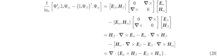
Next, let us consider an arbitrary 'annular' closed volume,  , with an inner surface,
  , exterior to the scattering system and an outer surface,
  , exterior to
  as illustrated in figure 2.

Figure 2. Annular volume,  , around a scattering system, with an inner surface,
  , surrounding the system and an exterior surface,
  , that will be sent to infinity.
Download figure:
Standard image High-resolution imageIntegrating over the annular volume integral and applying the divergence theorem to equation (20) yields:
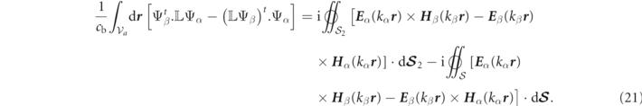
Letting the outer surface tend to infinity, the result can only be consistent with equation (19) provided that,

The vanishing of the surface integral,  , at infinity arises from distribution theory and is discussed at length in reference [16] and reviewed in appendix
  factor.
Equation (22) allows the orthogonality relation of equation (19) to alternatively be expressed as a volume integral over any finite closed region,  , containing the system, supplemented by an integral on the surface,
  , of
, of  :
:

For lossless particles, the medium metric, Γ, is frequency independent and real valued, so that equation (19) reads  , which for kα
≠ kβ
leads to a frequency independent eigenstate orthogonality condition for lossless systems:
, which for kα
≠ kβ
leads to a frequency independent eigenstate orthogonality condition for lossless systems:

which can of course also be expressed in the finite volume-surface form of equation (23).
It is worth remarking at this stage that the presence of the medium metric, Γ, gives a Lagrangian aspect to RS field products (as opposed to the more common Hamiltonian type products), which will become even more apparent when we consider RS normalization in section 2.4.
2.3.1. Regularizing multipole expansion products
Once the RS fields are developed according to equation (8), then the analytic expressions for RS product integrals, given in appendix

where the orthogonality of the VPWs over angular integration results in there being only a single sum over basis indices rather than the double sum that would generally occur using other basis functions. Analytic expressions for all the integrals on the right-hand side of equation (25) are given in equations (81a) and (81d) of appendix
Inside a homogeneous region, r < Rin, lying completely inside a scattering object (cf figure 1), one can again develop the RS field on a multipole basis according to equation (10), and the RS volume integrals are:

with ordinary analytic expressions for the integrals on the right-hand side of equation (26) being given in equations (82) and (83) of appendix
2.3.2. Orthogonalization: example with a spherical scatterer
Let us consider the case of a lossless sphere with relative permittivity, ɛ = 16 and null permeability contrast, μ = 1. A few low frequency electric mode RSs are graphically represented in figure 6 and given to high numerical precision in table 1. Since the sphere is lossless, the frequency independent RS orthogonality relation of equation (24) applies. This orthogonality relation requires that either the electric field and magnetic product integrals exactly cancel one another, or that they are both null. However, we know that for a system without material losses, knowledge of the electric field completely determines the magnetic field and vice versa, which leads us to the conclusion that RS orthogonality for dispersionless scatterers corresponds to the magnetic and electric field product integrals being independently zero. Rather than mathematically proving this statement, we next invoke the formulas of appendix
Table 1. RS eigenvalues, zα
, and associated residues,  , for a non-dispersive dielectric medium with dielectric contrast of ɛ = 16 and no magnetic contrast, μ = 1.
| α(q, n, [ℓ]) | zα |

|
|---|---|---|
| (e, 1, [1]) | 1.0395 − i0.500 935 | −0.236 682 + i0.231 492 |
| (e, 1, [2]) | 1.052 73 − i0.072 3549 | 0.065 9905 − i0.057 9972 |
| (e, 1, [3]) | 1.920 43 − i0.082 005 | 0.074 8408 − i0.028 2738 |
| (e, 1, [4]) | 2.7227 − i0.073 007 | 0.002 794 37 − i0.068 3107 |
| (e, 2, [0]) | −i1.679 7303 | i0.146 892 |
| (e, 2, [1]) | 1.377 484 − i0.011 8433 | 0.001 846 13 − i0.011 8059 |
| (e, 2, [2]) | 2.071 446 − i0.667 649 | −0.305 381 + i0.277 002 |
| (h, 1, [0]) | −i1.250 038 | i0.136 765 |
| (h, 1, [1]) | 0.753 7823 − i0.024 0302 | −0.006 017 59 − i0.022 9898 |
| (h, 1, [2]) | 1.541 4631 − i0.045 9254 | −0.039 4075 − i0.019 5948 |
| (h, 2, [1]) | 0.870 513 − i1.752 59 | −0.0521 306 + i0.140 046 |
| (h, 2, [2]) | 1.095 7165 − i0.006 840 25 | −0.000 482 964 − i0.006 816 78 |
Let us consider a magnetic field product of two distinct electric type RSs (q = 0) of a dispersionless spherical scatterer. Rescaling the radial variable by the sphere radius,  , a volume integral of the (complex valued) magnetic fields inside the sphere can then be evaluated as,


where equation (27a) is obtained after analytical integration of the angular variables, while the term in brackets of (27b) is a direct application of the bracketed integral in equation (27a) as given by equation (85a) of [16] (cf also Watson reference [48], and equations (78) and (82c)). The final result of equation (27c) exploits the expressions of equation (14a) for γα(e,n), and employs algebraic manipulations that are only true when zα and zβ are distinct RS size parameter eigenvalues (i.e. zα ≠ zβ ).
Thanks to the Gaussian regularization program, we find an analytic expression for integral in the region outside the sphere (where μ(r) = 1 due to medium normalization),


where we used equation (103a) in reference [16] to evaluate the integral in the first line of this equation (reproduced in equation (81e)). The 'killing' regularization, described in detail in reference [16] and appendix  factor in order to yield the finite analytic expression of equation (28b) in the η → 0 limit. We ignored irrelevant overall sign factors in the above demonstration because it is now clear that the integrals in equations (27c) and (28b) exactly cancel, so that indeed there is a magnetic field orthogonality of RS states in spheres for dispersion free media to yield,

where we stopped refering only to the field type index 'e' (q = 0) in equation (29) since as shown in appendix
In order to appreciate the complexity of what is accomplished in equation (29), the real and imaginary parts of a solid angle averaged RS magnetic product integrand of the first two electric dipole RSs at zα(e,n=1,ℓ=1) ≃ 1.0395 − i0.5009 and zβ(e,n=1,ℓ=2) ≃ 1.0527 − i0.072 355 of a high index dielectric sphere (ɛ = 16) are plotted in figure 3 (cf table 1 and figure 6). Specifically, the real and imaginary parts of the angle averaged magnetic field product integrands given in equation (27a) (r < R) and equation (28a) (r > R) are plotted first for r/R in figure 3(a), up to 1.2 and then extended in figure 3(b) up to values of r/R = 25, where a Gaussian killing factor of η = 0.025 is adopted for values of r > R. High accuracy numerical calculations confirm that the integrals of both the real and imaginary parts of the total magnetic field integral do indeed tend towards zero when a sufficiently small value of η in the region r/R > 1 is adopted.

Figure 3. Numerical plots of the RS magnetic inner product integrands of equation (28) (i.e.  ) for zα(e,n=1,ℓ=1) ≃ 1.0395 − i0.5009 and zβ(e,1,ℓ=2) ≃ 1.0527 − i0.072 355. The real (blue-solid) and imaginary (red-dotted) parts of equation (28), are plotted in (a) in the range (r ∈ {0, 1.2}) and for (r ∈ {0, 25}) with a η = 0.025 killing factor. Analogous plots for the electric field integrand of equation (89) are given in (c) and (d). The envelope of the curves when η = 0 is given by black dashed lines in (b) and (d).
Download figure:
Standard image High-resolution imageAnalogous result hold for RS orthogonality in terms of an electric field, despite presence of discontinuities in the electric field component normal to the scatterer surface. Analytical formulas for electric field orthogonality are given explicitly in appendix

when α ≠ β, a result which is illustrated graphically by plotting the electric field integrands of equations (89a) and (89d) for r/R up to 1.2 and figure 3(d) for r/R up to 25. As shown in appendix
An advantage of Gaussian regularization is that it can replace numerical integrations by analytical expressions (once the multipole development of the RS fields outside the system are determined). Although Gaussian regularization could also be used as numerical method, this may not be the most efficient choice for the following reason: a numerical evaluation of a Gaussian regularized RS integral should adopt a small value of η, so as to be close to the η → 0 limit, but small values of η lead to large amplitude far-field oscillations (cf figure 4), which renders numerical integrations time consuming. For numerical evaluations, it is often preferable to generalize the radial coordinate to complex values and deform radial integration path so that it goes to infinity at a finite angle from the real axis in the complex plane. This procedure is commonly employed in temporal analysis of applied mathematics and lies at the heart of the PML method [49].

Figure 4. Plot of the real part of equation (28) in the complex kr plane for η = 0.025. A Gaussian integration path along the real axis is given by the thick blue curve, while the red dashed curve indicates the path of a contour shifted by an angle of π/4 into the complex plane.
Download figure:
Standard image High-resolution imageWe can readily understand the numerical advantage of the complex contour method from figure 4, which plots the real part of equation (28), i.e. ![$\mathrm{R}\mathrm{e}\left[{r}^{2}{h}_{n}({z}_{\alpha }r){h}_{n}({z}_{\beta }r){\text{e}}^{-\eta {r}^{2}}\right]$](https://content.cld.iop.org/journals/1367-2630/23/8/083004/revision7/njpac10a6ieqn65.gif) (with η = 0.025) in the complex plane. The Gaussian regularized contour on the real axis is plotted as a thick blue line, while the red dashed curve indicates the path of a contour rotated by an angle of π/4 into the complex plane. The integrals along the two contours must be the same, but the red dashed PML type contour is clearly more manageable numerically and a Gaussian regularization is superfluous for the rotated path which could be evaluated directly without regularization (i.e. for η = 0). Although it is visually clear from figures 3 and 4 that RS product integrands oscillate around zero outside the scatterer, they do not quite average to zero since the RS orthogonality relation of equation (29) requires the exterior product integral to be equal and opposite to the field product integral inside the sphere, (this interior integral is generally not null, as seen in this example by inspection of figures 3(a) and (b)).
(with η = 0.025) in the complex plane. The Gaussian regularized contour on the real axis is plotted as a thick blue line, while the red dashed curve indicates the path of a contour rotated by an angle of π/4 into the complex plane. The integrals along the two contours must be the same, but the red dashed PML type contour is clearly more manageable numerically and a Gaussian regularization is superfluous for the rotated path which could be evaluated directly without regularization (i.e. for η = 0). Although it is visually clear from figures 3 and 4 that RS product integrands oscillate around zero outside the scatterer, they do not quite average to zero since the RS orthogonality relation of equation (29) requires the exterior product integral to be equal and opposite to the field product integral inside the sphere, (this interior integral is generally not null, as seen in this example by inspection of figures 3(a) and (b)).
The utility of analytic Gaussian regularization formulas is further highlighted by remarking that if one also evaluates the electric field product integrals (cf equation (89) in appendix

where the first term is a volume integral of fields inside a sphere of radius, R, denoted  , and the second term is a quantity evaluated at the sphere's surface. It is worth remarking that although R can be 'naturally' taken to be the particle radius, equation (31) remains valid for any sphere surrounding the scatterer.
An examination of equation (31) shows that the volume integral and the second, 'surface', contribution are none other than special cases (spherical volume and surface) of the more general volume and surface integrals derived in equation (23). Although the explicit agreement between the analytic Gaussian regularization method with equation (23) was only shown here for the case of a dispersionless sphere, analogous manipulations confirm this agreement for the case of dispersive spheres, at the cost of some additional algebra.
2.4. Resonant state normalization
A variety of methodologies have been adopted to determine RS normalization [24–27, 50], which has given rise to 'different' normalization conditions being proposed for photonic problems, but Kristensen et al [24] and others have argued that varying normalization formulas should be at least inter-consistent. We agree that final response functions of an RS theory should be independent of regularization schemes, but we saw when we adopted equation (7) for the Green function response, the 'correctness' of the RS normalization factors can be considered a matter of convention.
We found it advantageous to adopt a field theory based route to normalization and impose the RS norms in equation (7) be proportional to their associated RS frequencies, ωα , which since adimensional scalar products were desired, led us to adopt:

where we recall that zα
= ωα
R/c. Since the frequency derivatives of the constitutive factors in ![$\mathrm{d}\left[\omega \varepsilon (\boldsymbol{r},\omega )\right]/\mathrm{d}\omega $](https://content.cld.iop.org/journals/1367-2630/23/8/083004/revision7/njpac10a6ieqn67.gif) and
and ![$\mathrm{d}\left[\omega \mu (\boldsymbol{r},\omega )\right]/\mathrm{d}\omega $](https://content.cld.iop.org/journals/1367-2630/23/8/083004/revision7/njpac10a6ieqn68.gif) can be interpreted as accounting for the energy associated with material degrees of freedom [51], one can interpret the Lagrangian energy of the RS as
can be interpreted as accounting for the energy associated with material degrees of freedom [51], one can interpret the Lagrangian energy of the RS as  . The Lagrangian interpretation of equation (32), is more transparent in dispersionless media where it simplifies to:

Despite the divergence of RS field amplitudes, the infinite volume integrals in equation (32) can be regularized by either Gaussian regularization or by a PML type rotation of the integration path into the complex plane as illustrated in figure 4. Yet another way to determine the normalization factors is said to avoid the RS divergences by integrating only over a finite region of space, analogous to the formula found for RS orthogonalization in section 2.3. Indeed, it suffices to divide both sides of equation (23) by kα
− kβ
, and then take the limit kα
→ kβ
to obtain a finite volume expression of  being equal to a constant (which we assign as zα
), so that a finite volume normalization expression reads:
being equal to a constant (which we assign as zα
), so that a finite volume normalization expression reads:

where  is a finite volume surrounding the system and
  its surface. Although not necessary, we used k = ω/cb, to formulate equation (34) in terms of exterior medium wavenumber, k, (as opposed to angular frequency, ω). Several works in recent years have obtained formulas quite similar to equation (34)[25, 26, 50], but the formula with the most explicit agreement is equation (20) of reference [41], derived in the context a six-by-six component Green's function (except for a differing RS convention—obtained by replacing zα
on the right-hand side of equation (34) by 1).
its surface. Although not necessary, we used k = ω/cb, to formulate equation (34) in terms of exterior medium wavenumber, k, (as opposed to angular frequency, ω). Several works in recent years have obtained formulas quite similar to equation (34)[25, 26, 50], but the formula with the most explicit agreement is equation (20) of reference [41], derived in the context a six-by-six component Green's function (except for a differing RS convention—obtained by replacing zα
on the right-hand side of equation (34) by 1).
The frequency derivative (or k derivative) of fields in the surface integral of equation (34) could be deemed undesirable for numerical analysis, but we can take advantage of the scale invariance in the region outside the system to replace d/dk by  , as done in reference [41, 50]. Those favoring a surface integral approach to RS normalization often choose to formulate normalization in terms of volume integrals involving only the electric field (in contrast to the 'Lagrangian' field formulation of this work). One can transform from one formulation to the other by invoking a Poynting vector analysis which yields:

which in the case of null magnetic permeability contrast, i.e. μ → 1 allows the normalization constraint to be written in terms of an electric field volume integral:

where we used the replacement ![$\frac{\mathrm{d}}{\mathrm{d}\omega }{\left[\varepsilon (\omega )\right]}_{{\omega }_{\alpha }}\to 2\frac{\mathrm{d}}{\mathrm{d}{k}^{2}}{\left[\varepsilon ({k}^{2})\right]}_{{k}_{\alpha }^{2}}$](https://content.cld.iop.org/journals/1367-2630/23/8/083004/revision7/njpac10a6ieqn74.gif) . The surface terms in equation (36) are radial derivatives, and the first appearance of such a normalization in photonics seems to be have been derived in 2010 for dispersionless media [52].
. The surface terms in equation (36) are radial derivatives, and the first appearance of such a normalization in photonics seems to be have been derived in 2010 for dispersionless media [52].
Even though the normalization formulas of equations (32), (34) and (36) may appear distinct from one another, the Gaussian regularization perspective shows their equivalence, under the proper conditions, since they are all determined by the same underlying condition. This equivalence can be demonstrated directly for a spherical surface,  , of radius R by using Hankel function recursion relations to show that the surface integral on the right-hand side of equation (34) of an arbitrary spherical surface of radius R is analytically identical to the formula of equation (94) for a Gaussian regularized volume integration of the electromagnetic field carried out in the region outside this sphere. Such analytic equivalencies can also be extended to arbitrary scatterer geometries by invoking the multipole decomposition of equation (8).
2.4.1. Analytic formulas for fully dispersive spherical scatterers
Analytical RS normalization expressions are derived in appendix


with the definitions:


For dispersionless media, light scattering becomes scale invariant and equation (37) simplifies to expressions which only depend on the size parameter of the mode, zα , and the relative constitutive parameters, ɛ and μ (now real-valued) as was previously derived in reference [17]:


Comparisons of the above normalization formulas for spherical scatterers with other analytic formulations are discussed in appendix
It is insightful to plot the radial dependence of the normalization integrals of equation (33) (after angular integration) for a lossless dielectric of ɛ = 16 as shown in figure 5. The convergence factor was simply set to η = 0 in these graphs since the exponential divergence only becomes relevant for r/R significantly larger than the r/R < 4 range in the RSs plots for the z2, z3, and z4 RSs. For such low loss RSs, a numerical 'verification' of equations (33) or (32) is simple because the exponential divergence only becomes non-negligible after passing through a long region where the integrand is nearly zero. Therefore, truncations of the low loss RS integrals will approximately verify equation (33) as one can guess by visual inspection of figures 5(b)–(d).

Figure 5. RS normalization integrand real parts (blue) and imaginary parts (red) for the first four electric dipole RS size parameters, zα(e,n=1,ℓ=1,2,3,4) plotted as functions of r/R with a null killing factor (η = 0) in the case of a dielectric sphere with high permittivity (ɛ = 16).
Download figure:
Standard image High-resolution imageThe situation is quite different however for poorly confined RSs with large imaginary parts, like z1 ≃ 1.04 − i0.5. As one can see in figure 5(a), the exponential divergence sets in immediately outside the sphere and a regularization of the RS normalization is essential if we look to numerically reproduce the analytic normalization result of equation (33). Similar behavior is observed for the RSs of lossy scatterers studied in section 4.3 below.
Unlike the physics of closed systems, where the phase of the modes can often be treated as arbitrary, the RS 'normalization' factors,  , must correctly adjust the phase of the RSs which is a crucial information for reconstructing response functions. This point will be reinforced in section 3, where we will see that the RS phase determines the complex residues in spectral developments of response functions.
The ultimate justification for setting the right hand sides of equations (32), (34) and (36) to zα
, is that this choice generates particularly simple spectral response functions presented in section 3 below. A more widespread choice is obtained by defining a rescaled RS wavefunction  for which the RS normalization reads:

which is reminiscent of normalization in closed systems like conventional quantum mechanics.
2.4.2. Mode volumes
Recent derivations of the Purcell factor for RSs define a mode 'volume', Vα [23, 24, 26, 39, 53]. These derivations generally invoke a Green's function formalism and the local density of states (LDOS), which generally leads to a 'complex' valued mode volume [54–56]. A typical definition for Vα derived along the LDOS Green function approach is:

where
r
c is a 'chosen' position (often the field maxima) while  is one of the commonly employed photonic notations [24] for the RS electric field, and the double '⟨⟨...⟩⟩' is an inner product notation reference [24]. Following the usual LDOS route to mode volume in the framework of this work leads to,

which up to possible proportionality factors agrees with more recent mode volume definitions that continue to be debated even now [57].
As discussed in the previous paragraph and the references therein, given that Vα
is generally complex valued, there appears to be little utility in trying to interpret it as a true mode 'volume', and it is generally considered preferable to interpret it as the inverse normalized field squared. Mode volume assignments along the lines of equations (40) and (41) tell us that |Vα
| is proportional  , so we generally expect small values of
  to correspond to 'small' mode volumes, or in other words, stronger interactions with an incident field. One indeed sees from table 2 that poorly confined, 'structural' modes like
  (cf figure 5(a)) have smaller
  , than the more 'resonant' modes illustrated in the other graphics of figure 5.
Table 2. Illustrative electric dipole RSs, α(e, n = 1, ℓ), for plasmonic particles: for the dispersion models of equations (52b) and (53) for gold and equation (52a) for silver. The complex wavelengths and dielectric constants are given in addition to the Mie coefficient residue factor,  , associated with RS normalization is given in the last column.
| R (nm) | ℓ | Disp. | λα (nm) | ɛα |

|
|---|---|---|---|---|---|
| 100 | 1 | (52b) | 606.976 + i239.112 | −13.7606 − i12.5419 | −0.217 942 + i0.034 889 |
| 100 | 1 | (53) | 592.219 + i210.126 | −5.904 24 − i12.9379 | −0.309 192 − i0.005 709 58 |
| 80 | 1 | (52b) | 505.163 + i174.433 | −9.480 69 − i7.588 28 | −0.2111 − i0.003 857 08 |
| 80 | 1 | (53) | 547.731 + i79.8811 | −3.642 00 − i3.522 01 | 0.017 306 − i0.100 09 |
| 100 | 1 | (52a) | 600.211 + i231.333 | −11.1356 − i14.0631 | −0.236 629 + i0.026 6621 |
| ⋅ | 2 | ⋅ | 290.678 + i33.6325 | 0.704 812 − i0.966 352 | 0.178 962 + i0.124 692 |
| ⋅ | 3 | ⋅ | 217.845 + i20.8224 | 2.580 05 − i0.449 824 | 0.013 9492 − i0.235 957 |
| 80 | 1 | ⋅ | 500.306 + i156.443 | −6.780 66 − i7.895 19 | −0.235 268 − i0.050 9908 |
| ⋅ | 2 | ⋅ | 281.965 + i50.9047 | 1.030 36 − i1.441 87 | 0.127 46 + i0.248 96 |
| ⋅ | 3 | ⋅ | 192.72 + i20.4675 | 3.110 19 − i0.394 101 | 0.103 72 − i0.210 644 |
Inspection of equation (38) appears to lead to the conclusion that weak constitutive contrasts lead to small values of  ). However, the
  factors in equation (38) do not at all vanish in the limit of zero contrast since the vanishing (ɛ − 1) and (μ − 1) factors, are multiplied by factors expressed in terms of spherical Hankel functions evaluated at the RS frequencies. The fact that the
  normalization factors remain finite in the limit of null contrast is in fact a necessary ingredient for retrieving a vanishing T-matrix response, (cf section 3), in the zero contrast limit. A detailed analysis of this intriguing result will be addressed elsewhere.
3. Resonant state expansions of Mie theory response functions
One can obtain physical response functions directly from the Green's function, but we have argued in recent years the advantages of employing elegant and powerful scattering formalisms involving S and T-matrices and reaction matrices (cf [17, 18, 22, 37–39] for more details and applications). An essential idea is seen by remarking that the T-matrix operator,  , is related to the Green's function as: [58–62]

where  is the Green function of the homogeneous background. An advantage of this formalism is that the
  -operator describes electromagnetic response in terms of fields (as opposed to source current for Green's functions). This occurs because the
  operators on the left and right side of
  in equation (42) respectively generate outgoing and incident multipole fields, (the normalization in equation (32) accounts for differences in the fields generated by
  operators and the conventional multipole fields) [47, 58, 61]. Once projected onto the multipole basis, the
  -'operator' takes the form of a 'matrix' on the multipole basis functions (which is precisely the justification of the terminology T-matrix).
Given the observations made around equation (7) and in the previous paragraph, we conclude that the RS residues of the scattering T-matrix are  , as will be confirmed below for spherical scatterers, since the T-matrices in this case are diagonal on the multipole basis (with matrix elements given analytically by Mie theory for complex frequencies). This agreement is remarkable in that
  was obtained through RS regularization, quite outside the context of traditional Mie theory. Although it is clear from equation (42) that T-matrices are just a reformulation of the Green function of equation (7), we have found in our prior works that the T-matrix formulation has the advantage of facilitating the derivation of the non-resonant contributions to response functions [17, 18, 22, 37–39] (notably through considerations of causality and energy conservation [21]). Relevant results of this approach, and some new derivations in the context of RS Mie theory, are reviewed below.
3.1. RS spectral expansions
In the interest of completeness, essential elements of Mie theory and linear response theory are recalled in appendix
The meromorphic expansion of the Tn functions in terms of frequency, ω, have been determined to be [17, 18, 22, 37]:


which takes the form of a non-resonant contribution to which one adds the spectral RS contributions. (zα = kα R with α(q, n, ℓ) being determined by multipole indices, q, n, and the discrete RS index, ℓ). The question mark on the truncated RS approximation in equation (43b) highlights the fact that the obligatory truncation of an infinite RS sum should be addressed with care (see the end of this section and section 4.4 for further discussion).
Recent works have proposed to derive the non-resonant contributions by summing static-mode contributions [42, 43], but we have found it more expedient to determine the non-resonant contributions analytically by invoking mathematical constraints derived in the context of the S/T-matrix response functions [17, 18]. An advantage of our formulation is that it holds true even for Drude-type constitutive parameters where static mode formulations do not appear to be applicable. The relationship between these approaches appears to merit further investigation [43].
The first, non-resonant, term on the right-hand side of equation (43) is a function of only the particle size parameter, z = kR = ωR/c. The Aq,n in equation (43), are multipole sign factors, which for q = 0 (magnetic) or q = 1 (electric), modes are:

The residues, rα , of the RSs in the RS expansion of the T-matrix in equation (43) are,

where the  phase factor does not affect the T-matrix residue equation (43) since it is canceled by the e−2iz
multiplicative factor so the RS residues are indeed
phase factor does not affect the T-matrix residue equation (43) since it is canceled by the e−2iz
multiplicative factor so the RS residues are indeed  as expected.
The internal field coefficients of Mie theory, Ωq,n , are quite similar to the T-matrix expressions with the exception of their response being expressed entirely in terms of RS states, (i.e. there are no non-resonant contributions):

As one could deduce from equation (7) and the RS expression in equation (16), the residues of internal RS coefficients, are related to the T-matrix residues in equation (46), as  .
.
Since the non-resonant contributions were determined analytically here, we could expect to be able to retrieve the Mie coefficients from the RS spectral expansion in equation (43), but upon closer inspection we realize that there is no reason to presume that the neglected, high frequency, RSs will make negligible contributions to the Mie coefficients (which up to a sign difference are matrix elements of the T-matrix which in turn is a reformulation of the Green's function—as seen in equation (42)). In order to demonstrate this lack of 'convergence', we developed codes that determined the RSs in a given frequency window, and one of our initial 'solutions' to the convergence problem, for dielectrics, was to simply to include hundreds of RSs when reconstructing Mie coefficients using equation (43b).
We should keep in mind however that the initial interest of RSs was to characterize a physical system with a modest number of relevant RSs, and the necessity of including hundreds of RSs in spectral expansions would considerably diminish the utility of this formulation, particularly in the case of non-spherical objects where the asymptotics of high frequency RSs will be less straightforward. This convergence difficulty turned out to be even more problematic when treating dispersive scatterers as we will see in section 4.4.
3.2. Spectral residues in Mie theory
Given the expressions for Ωn
, and Tn
in section 3.1 and equation (46) in terms of the Nq,n
and Dq,n
functions defined in equations (86) and (87) of appendix

which can be rewritten as,

One should note that for non-dispersive media, the scale invariance of the underlying electromagnetic equations imposes that the residues, rα
and  , only depend on particle radius, R, as a function of, zα
= ωα
R, which results in the spectral response functions of equations (46) and (43b) becoming solutions for all particle sizes and frequencies in this case.
, only depend on particle radius, R, as a function of, zα
= ωα
R, which results in the spectral response functions of equations (46) and (43b) becoming solutions for all particle sizes and frequencies in this case.
We remark from the second equality in equation (47b) that the relation between the T-matrix residues, rn,α
, and the internal field residues,  , is purely analytic. This relation can be rewritten in a more transparent form by invoking the respective RS conditions of equation (14) such that the expressions of Ne,n
and Nh,n
can be rewritten:
, is purely analytic. This relation can be rewritten in a more transparent form by invoking the respective RS conditions of equation (14) such that the expressions of Ne,n
and Nh,n
can be rewritten:

for the electric modes and,

for the magnetic modes. In both equations (48a) and (48b) we invoked the Wronskian relation,

and recalled the definitions of the γα functions defined in equation (14).
Mie theory therefore analytically validates the relation,

that we deduced after equation (46) using arguments based on RS spectral expansions of the response function. Although the derivation is a bit lengthy here, one can also directly derive the T-matrix residue,  , directly from Mie theory. We found this fact quite striking since Mie theory makes no use whatsoever of the RS regularization methodology. We interpret this as striking evidence for the mathematical validity of the RS regularization program.
4. Numerical implementations
This section provides precise calculations of RS eigenvalues, normalization, and response function reconstructions in the case of spherical scatterers. As discussed in section 2, generalizations to non-spherical shapes are quite analogous, but they will not be considered here since they are not amenable to such high precision analytics.
Even for spherical geometries, solving for the RS frequencies must be carried out numerically, but thanks to the field continuity conditions of equation (14), the RS frequencies are determined as solutions to analytic expressions that can be expressed in terms of the reduced logarithmic derivatives of the Ricatti–Bessel functions:


where we recall from equation (15) that ɛα , μα , and ρα are in general frequency dependent constitutive parameters evaluated at the RS frequency, ωα , such that the first terms in equation (51) have a non-trivial frequency dependence.
4.1. Resonant states and normalizations of high refractive index dielectric spheres
There is currently considerable interest in non-dispersive scatterers since high index dielectrics are being considered in nano-optics as an alternative to plasmonics [63]. Even for such energy conserving systems, one still needs to solve equation (51) numerically, but the difficulty is greatly reduced and the problem becomes scale invariant, which means that one essentially solves the problem for all particle sizes and/or frequencies simultaneously. Furthermore, the RS normalization coefficients are calculated with the simple expressions found in equation (38).
Numerical results for a few low-order modes of a dielectric with no magnetic permeability contrast, μ = 1 and high, ɛ = 16, permittivity contrast are shown in table 1 (further analysis and discussion of such modes may be also found in [18]). There are an infinite number of modes for each value of n, and they follow an asymptotic pattern resembling that of zeros of Bessel functions. Beginning with electric modes, table 1 gives the values of zα
and the normalization factors for the first two dipole and quadrupole modes. An interesting feature of the RSs in this case is that for n even (odd), there is one electric (magnetic) mode with purely imaginary z, labeled with ℓ = 0. One can also remark from table 1 that for imaginary RS eigenvalues, the interaction 'strengths' (residues),  , have purely imaginary values.
The high number of significant figures given in table 1 for the RS eigenvalue size parameters, zα
and normalizations,  were adopted because these values were indeed calculated up to such high order accuracy which underscores the results of this work to serve as benchmarks for more numerically based approaches.
4.2. Numerical verification of RS expansions of Mie theory
The steps to implement the results of this paper up to the construction of Mie theory response functions can be summarized as follows:
- (a)For each required multipole order n, and mode type q = (0, 1), (i.e. (h) and (e) respectively), the only non-trivial step is to find a sufficient number of the RS size parameters, zα , by numerically solving the transcendental equation (14) (or equivalently equation (51)). The sufficient number of RSs depends on the particle radius R (or frequency of interest) and the dispersion relations of the constitutive parameters, but might be as low as 1 for some applications in dispersive materials. When only a few RSs are required, graphical solutions with numerical refinements may suffice (see section 4.3 for examples, but one should exercise caution with such techniques since important RSs can occur far from the real z axis as can be seen in figures 6(b) and (e)).
- (b)Calculate the square of the complex-valued RS norms,
 , using equation (37).
 - (c)Insert the values of found in step (b) into equation (45) to determine the residues, rα(q,n,ℓ), for the meromorphic expression of section 3.1 for the scattered field Mie coefficients, an
= −Te,n
and bn
= −Th,n
. Cross section contributions, σn
, can then be determined by the standard formulas recalled in equation (88) of appendix
D.2 . - (d)If one needs to determine the fields inside the sphere, use the values of rα found in step (c) and the γα(q,n,ℓ) coefficients of equation (14) to calculate the residues,, of equation (50) that appear in the meromorphic expression of equation (46), for the internal field Mie coefficients cn
= Ωh,n
and dn
= Ωe,n
(defined in equation (85b)).


The results displayed in table 1 of section 4.1 were obtained by applying steps (a) and (b) above. An illustration of carrying out step (c) above, with the same material parameters (ɛ = 16, μ = 1) used in figure 5, is illustrated graphically for both electric and magnetic mode contributions and orbital quantum numbers, n = 1 and n = 4. The first few RSs for each mode are given as blue dots in the lower half plane with Im(z) on the vertical axis, while the associated contributions to the cross section efficiencies, Q ≡ σ/(πR2), are plotted on the positive vertical scale. In figures 6(c) and (f), we verified that this procedure reproduces Mie theory up to arbitrary computational accuracy for all multipole orders when large numbers of resonant states are included.

Figure 6. The electric RSs and their contributions to cross-sections for multipoles, n = 1 and n = 4 for a dispersionless sphere with ɛ = 16: electric modes (a) and (b) and magnetic modes (c)–(f). The geometrically normalized cross section contributions,  , are plotted according to the positive vertical axis. Complex RSs are indicated by blue dots with Im(zα
) on the negative vertical axis. In parts (c) and (f), the contributions of the n = 1 (red) and n = 4 (green) multipoles are compared with the total cross section (blue line) determined by the sum of all multipole contributions for the electric and magnetic cases respectively.
, are plotted according to the positive vertical axis. Complex RSs are indicated by blue dots with Im(zα
) on the negative vertical axis. In parts (c) and (f), the contributions of the n = 1 (red) and n = 4 (green) multipoles are compared with the total cross section (blue line) determined by the sum of all multipole contributions for the electric and magnetic cases respectively.
Download figure:
Standard image High-resolution imageThe curves in figure 5 were generated both from RS calculations and Mie theory, but are identical since they agreed here up to six figure accuracy, but at the cost however of including hundreds of RSs in equation (43). Similar calculations can reproduce Mie theory for dispersive media, but in that case, the problem is no longer scale invariant and the position of the RS eigenfrequencies will depend on the particle size and will be seen in section 4.3 below.
4.3. Resonant states and normalizations of 'Drude' model conductors
The calculation of the complex wavenumbers of RS's depends on an extrapolation of the experimental data on complex permittivities (or permeabilities in cases involving magnetic materials) from the real axis of frequencies or wavelengths. Such an extrapolation depends critically on both the accuracy of the experimental data and on the accuracy of the analytic model used for the extrapolation.
Data on the complex refractive index of gold as a function of frequency are available in volume 1 of the comprehensive collection due to Palik [64]. The simplest widely used analytic expression for this data is that of the Drude model, which may be written in terms of the angular frequency, ω, for gold [23] and silver [65] as:

The comparison with experimental data given in figure 13 of appendix
To achieve a better fit for gold valid down to shorter wavelengths, extra Lorentz resonant terms need to be added to the Drude model of equation (52b). For example, Sikdar and Kornyshev [66] give the parameters for a model for gold taking into account inter-band transitions via two additional resonances:

Here the parameters are given in eV:  ∞ = 5.9752, ℏωpD
= 8.8667 eV, ℏΓD
= 0.037 99 eV, s1 = 1.76, ℏωp1,L
= 3.6 eV, ℏΓ1,L
= 1.3 eV, s2 = 0.952, ℏωp2,L
= 2.8 eV and ℏΓ2,L
= 0.737 eV. The conversion of ω to electron volts is achieved by dividing the frequency results by e/ℏ = 1.519 27 × 1015. As can be seen from figure 14, this model works well down to around 0.40 μm. An interesting feature of the dispersion model of equation (53) is that it supports bulk plasmons [67]. These occur for complex wavelengths or frequencies at which ɛ(ω) = 0. For the dispersion model of equation (53) they are at: λLg = 0.257 778 + i0.020 6709 μm, λLg = 0.395 618 + i0.053 6046 μm, λLg = 0.502 518 + i0.048 786 μm. Bulk plasmons are longitudinal waves, which do not couple to transverse electromagnetic waves and cannot be excited by or scattered into them. This translates as the fact that one obtains a normalization residue factor,
∞ = 5.9752, ℏωpD
= 8.8667 eV, ℏΓD
= 0.037 99 eV, s1 = 1.76, ℏωp1,L
= 3.6 eV, ℏΓ1,L
= 1.3 eV, s2 = 0.952, ℏωp2,L
= 2.8 eV and ℏΓ2,L
= 0.737 eV. The conversion of ω to electron volts is achieved by dividing the frequency results by e/ℏ = 1.519 27 × 1015. As can be seen from figure 14, this model works well down to around 0.40 μm. An interesting feature of the dispersion model of equation (53) is that it supports bulk plasmons [67]. These occur for complex wavelengths or frequencies at which ɛ(ω) = 0. For the dispersion model of equation (53) they are at: λLg = 0.257 778 + i0.020 6709 μm, λLg = 0.395 618 + i0.053 6046 μm, λLg = 0.502 518 + i0.048 786 μm. Bulk plasmons are longitudinal waves, which do not couple to transverse electromagnetic waves and cannot be excited by or scattered into them. This translates as the fact that one obtains a normalization residue factor,  , of zero for any longitudinal 'RSs'.
Figure 7 shows the modulus of the dispersion equation of equation (51a) for n = 1 and for a gold sphere of radius 100 nm, both for the Drude model of equation (52b) and for the more elaborate Drude-Lorentz model of equation (53). The former has its minimum at λα = 0.606 976 + i0.239 112 μm, in good agreement with the value reported in Sauvan et al [23]. The latter has a slightly different value: λα = 0.592 227 + i0.210 097 μm. From table 2 the values of ɛα at the resonance and consequently the normalization factor disagree more significantly for the more elaborate model.

Figure 7. The inverse of the modulus of the dispersion equation (51a) for the electric dipole mode of a gold sphere of radius 100 nm and an RS at λα ≃ 607 + i239 nm. (Left) The Drude model of equation (52b); (right) the extended Drude–Lorentz model of equation (53) with a lowest energy RS of λα ≃ 592 + i210 nm.
Download figure:
Standard image High-resolution imageFigure 8 shows the inverse modulus of the n = 1 dispersion relation of equation (51) for a gold sphere of radius 80 nm. The plot is more complicated for the more elaborate dispersion model of equation (53) since the decrease in radius moves the wavelength range of interest into that for which the zeros, poles and branch cuts of this dispersion model become evident (see the data listed above for the wavelengths corresponding to bulk plasmons). The complex wavelength of the RS for the Drude model is λα = 0.505 163 + i0.174 433 μm. With the model of equation (53), this becomes λα = 0.547 815 + i0.080 062 μm. Note the significant decrease in the imaginary part around this wavelength, as visible in figure 14, since the Drude model is only a crude approximation to the experimental data.

Figure 8. The inverse of the modulus of the n = 1 dispersion equation, (equation (51a)) for a gold sphere of radius 80 nm. (Left) The Drude model of equation (52b) with and a principal RS at λα ≃ 505 + i174 nm. (Right) The model of equation (53) with a lowest energy RS of λα ≃ 548 + i80 nm.
Download figure:
Standard image High-resolution imageThe aforementioned electric dipole RSs for the different dispersion models are given in table 2 for RSs in silver and gold spheres of radius 100 and 80 nm. In order to calculate the mode normalization factors, the numerical differentiation, described in equation (47), is a valid alternative to equation (37) for finding the necessary dispersion derivatives. The data given in table 2 for the resonances of silver spheres of radius 100 and 80 nm shows complex wavelengths and normalization factors which are broadly similar to the corresponding values for gold.
4.4. Response function with truncated RS spectral expansions
We argued at the end of section 3.1 that one cannot necessarily expect the Mie coefficients of equation (43a), with their infinite sets of RS poles, to be accurately approximated by the directly truncated RS sums in equation (43b). In order to better understand this issue, let us first see what happens if we adopt the direct truncation of equation (43b) for a particularly simple physical example. Specifically, let us adopt the gold Drude model of equation (52b) and an R = 80 nm sphere, for which a well isolated 'principal' RS is illustrated graphically in figure 8 (and given numerically in table 2-line 3). This isolated, long wavelength RS has the promising property of lying near the broad, red-shifted plasmon 'resonance' peak in the electric dipole extinction cross section,  , calculated from Mie theory and plotted as the solid blue lines in figures 9(a) and (b).

Figure 9. Extinction cross section for an R = 80 nm gold sphere plotted using a simple Drude gold model of equation (52b). In (a), we plot the exact Mie theory calculation as a solid blue curve, while the 'directly' truncated model with Lmax = 1 is plotted as a dotted green curve and the 'corrected' normalization deduced from equation (54) is plotted as a dashed red curve The second graphic, (b) is the same as (a), but with the truncated calculations carried out for Lmax = 4.
Download figure:
Standard image High-resolution imageDespite the apparent simplicity of the physical situation, truncating the RS expansion in equation (43b) to a single independent RS state is far from being satisfactory (dotted green curve in figure 9(a): Lmax = 1). If we try to 'improve' the approximation by adding additional RSs, as shown by a Lmax = 4 calculation in figure 9(b) (dotted green curve) the agreement only worsens and quickly loses any semblance of physical relevance with predictions of large negative cross sections and unitarity violations. A solution to this problem will be described in the following paragraphs, and the results of this new, 'optimized', truncation technique are plotted as dashed red curves in figures 9(a) and (b) for Lmax = 1 and Lmax = 4 respectively. The word 'optimized' is used to indicate that this improved methodology tends towards the exact results with increasing values of Lmax as desired.
The cause for the 'failure' of the direct spectral expansion was traced to the fact that the Mie coefficients resulting from the 'infinite' RS series, has an analytic structure that a direct truncation of the RS series in equation (43) (using analytic normalizations/residues) does not preserve. One can solve this problem by constraining the truncated RS spectral expansions to satisfy the same unitarity requirements as the exact Tq,n
function deduced from Mie theory. This was done by appealing to the S-matrix, related to the T-matrix by  , (
, ( being the identity operator). The key observation is that the zeros of the S-matrix, denoted
  , satisfy the same equation as the RSs, i.e. equation (4), but with incoming boundary conditions replacing the outgoing RS boundary conditions (in equations where the RS eigenvalues also appear, the RS eigenvalues will be denoted
  ). For lossless dielectrics, the
  are simply the complex conjugates of the RS eigenstates,
  , but for dispersive materials the set of
  values must be determined anew by solving the self-consistent eigenvalues with incoming boundary conditions (n.b. unlike the RSs,
  , which have only non-positive imaginary parts,
  may be either positive or negative for dispersive scatterers).
The S-matrix can then be conveniently expressed in terms of eigenvectors of  , and
, and  . For spherically symmetric particles, this leads to a particularly convenient, alternate expression for the response function residue, rα
, formulated entirely in terms of
. For spherically symmetric particles, this leads to a particularly convenient, alternate expression for the response function residue, rα
, formulated entirely in terms of  , and
, and  :
:

where the poles (i.e. RS normalization as seen in equation (45)) can now be approximately determined as a function of a finite number of poles and zeros bounded by Lmax (which we take to be the same as the truncation adopted in equation (43b)).
We numerically verified that for |ℓ| ≪ |Lmax|, the approximate equality in equation (54) tends toward the analytic results of equation (45) for increasingly large values of Lmax, but that for RSs near the cutoff (ℓ ∼ ±|Lmax|), rα differ significantly from the analytically calculated values. The advantage of this cutoff 'corrected' construction of the residues is that it enforces 'optimized' analytic behavior and static limits on the truncated Mie coefficients of equation (43b) at any truncation level, Lmax, which thereby enables the RS expansion to converge to the Mie result. We plot the complex wavelengths of the first 25, positive wavelength, RSs of an R = 80 nm sphere in figure 10(a) for the simple Drude model of gold, equation (52b), and the more complex Drude–Lorentz model of equation (53), in figure 10(c). The results of the convergent RS expansion method with Lmax = 25 are then plotted as red dashed curves in figures 10(b) and (d) respectively. This truncation level suffices to produce approximate curves that are almost indistinguishable from the exact (solid blue) curves. Similar agreements can be found for any multipolar order and thus allow Mie theory to be completely reconstructed within the RS framework for both dispersive and non-dispersive scatterers.

Figure 10. The first 25 RS wavelengths, λα
(blue dots), for an R = 80 nm gold sphere are plotted in (a) and (c) using two different dispersion models (the simple Drude gold model of equation (52b) in (a) and the Drude–Lorentz model of equation (53) in (c). Electric dipole (Mie) contributions to extinction cross section,  , for these two models are plotted as solid blue curves in (b) and (d). Calculations with the convergent residue method of equation (54), using Lmax = 25, are plotted as dashed red curves. Dotted green curves correspond to the same RS calculations as for the red curves, but with the non-resonant contributions of equation (43) artificially set to 0.
Download figure:
Standard image High-resolution imageFinally, it is crucial to remark that the convergence towards the Mie theory results was only possible because we had added the analytically determined non-resonant contribution to the RS spectral expansion in equation (43). Ignoring the non-resonant terms would again lead to catastrophic predictions (notably negative cross sections), as illustrated by the dotted green curves in figures 9(b) and (d) where we used the same convergent RS expansion as the red dashed curves, but where the non-resonant contributions were arbitrarily set to zero.
It is widely recognized that the plasmonic resonances can be viewed as a collective quasi-static excitation, so it therefore appears physically relevant that the non-resonant term, determined from quasi-static considerations, plays such a major role in metallic scattering. Such 'plasmonic' resonances are thereby rather different from their dielectric counterparts which tend to have their principal cross section peaks dominated by RS contributions (despite the continued importance of non-resonant contributions [17, 18, 22]).
5. Conclusions and perspectives
We used Gaussian regularization to demonstrate that RSs can be assigned finite normalization and orthogonality properties that are closely analogous to definitions adopted for the eigenstates of closed systems. A notable difference however is that the RS normalization factors,  , are complex valued, (in contrast to their real-valued counterparts in closed systems). Although, 'irrelevant' phase factors are a familiar feature of the time evolution of eigenstates in dispersionless closed systems, phase plays a crucial physical role in an open system's response to an external excitation (and consequently can no longer be treated as arbitrary). The RS normalization factor must therefore ensure the physically correct RS phase, in addition to its amplitude. Recognizing the importance of phase factors from the outset helps one to understand the fact that when RS physics is imposed on closed system concepts, like the Purcell factor, the complex normalization factor inevitably leads to the introduction of apparently incongruous notions like complex valued mode volumes [24, 56, 57].
For systems of arbitrary geometry, the determination of the RS eigenvalues and the regularization of their inner products are often carried out numerically. This work combined a multipolar expansion of arbitrary RSs with Gaussian regularization in order to analytically evaluate the inner product integrals in the region lying outside the system of interest. Our analytical analysis can serve both as benchmarks for purely numerical treatments, as shown in section 4, and also increase the speed of numerical approaches by replacing certain numerical integrals with analytical formulas. The results of this work for RS normalization have been shown to be consistent with other formulas in the literature for non-spherical scatterers and we have explicitly generalized previous analytical results of the literature for dispersive spherical scatterers with both permittivity and permeability contrasts.
The Gaussian methodology introduced in this work was used to illustrate the difficulties of constructing spectral expansions of response functions. The problem of requiring non-resonant terms in RS spectral expansions has been addressed before [17, 18, 22], and has continued to be the subject of investigations [42, 43], but the importance of correcting the RS 'normalizations' in order to ensure the analyticity of truncated RS spectral expansions is a new finding. Both of these 'difficulties' were resolved here for the special cases of spherical dispersive and non-dispersive scatterers, but the methodology introduced should prove generalizable to arbitrary geometries and will be the subject of future studies. The utility of this work for spherical scatterers should not be dismissed however, because given the vast popularity and practical utility of Mie theory in applications, there can be little doubt that the ability to reliably formulate Mie theory in terms of the conceptually and mathematically simple RS spectral expansions will find future, and likely unforeseen, applications and insights.
Acknowledgments
Research conducted within the context of the International Associated Laboratory for Photonics between France and Australia (LIA ALPhA). This work has been carried out thanks to the support of the A*MIDEX Project (No. ANR-11-IDEX-0001-02) funded by the Investissements d'Avenir French Government program, managed by the French National Research Agency (ANR). We would like to thank Jean-Paul Hugonin for calling our attention to the numerical equivalence between the Gaussian normalization and the PML deformation into the complex plane as demonstrated in figure 2. We would also thank the referees whose remarks helped improve this manuscript, most notably concerning notation and more thorough the comparisons with results in literature.
Data availability statement
All data that support the findings of this study are included within the article (and any supplementary files).
Appendix A.: Alternative normalizations and literature comparisons
Given the wide variety of constantly evolving notations and conventions in the QNM/RS literature, it is not realistic to carry out exhaustive comparisons, so in this appendix we show that our normalization formulas agree with other analytic formulations in the special case of purely dielectric scatterers that have previously been given in the literature, notably those by Muljarov et al and in particular in references [26, 50].
Although we adopted a six component electromagnetic field formulation in contrast to the more common formulations entirely in terms of the three-component electric field, such differences should not affect the values of RS normalization. One remarks that reference [50] labeled RS indices 'n' as opposed to our generalized index α, and they used an index, ℓ, for multipole number as opposed to our 'Mie theory' choice of index n. Comparisons between our formulas and those given in references [26, 50] are facilitated by introducing the definitions of reference [50]. These authors used radial dependent constitutive parameters of a spherical scatterer are defined as:

and defined a function Rn :

together with

where the various spherical Bessel functions, jn , ψn , hn , and ξn are defined here in appendix B.
Invoking our definitions of equation (14) together with the RS relations for spherical scatterers in equation (51), our six component RSs equation (16) can finally be compactly reexpressed:
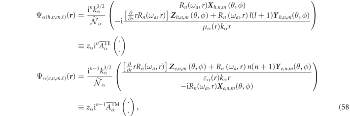
where the final set of parentheses are identical to the parenthesis of the central expressions; thus establishing the connection between the normalization coefficients  and
and  of reference [50], with our normalization factors,
  . Note that we normalized the coefficients of reference [50]
  , in order to compensate for the
  normalization factor of spherical harmonics that was included in our vector spherical harmonics
X
q,n,m
,
Y
q,n,m
, and
Z
q,n,m
, given in appendix B (also note that
normalization factor of spherical harmonics that was included in our vector spherical harmonics
X
q,n,m
,
Y
q,n,m
, and
Z
q,n,m
, given in appendix B (also note that  reads
reads  in reference [50]).
The electric fields in the parenthesis of equation (58) can be directly identified with the RS electric fields in equations (26) and (27), of reference [50] (again up to the  factor). In order to make our RS fields of equation (16) match the RS field expressions of reference [50], we had to divide our multipolar fields Φα
by hn
(zα
), which we then had to compensate for via a modified normalization factor,
factor). In order to make our RS fields of equation (16) match the RS field expressions of reference [50], we had to divide our multipolar fields Φα
by hn
(zα
), which we then had to compensate for via a modified normalization factor,  :
:

which results in particularly compact and symmetric expressions:
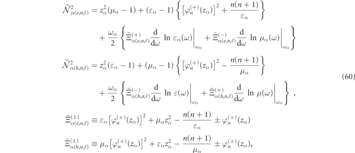
where  is the reduced logarithmic derivative of the outgoing Riccati Hankel function, ξn
(z):
is the reduced logarithmic derivative of the outgoing Riccati Hankel function, ξn
(z):

Finally, we remark that we had to multiply the Aα
coefficients of reference [50] by an additional zα
factor in order to account for the fact that we normalized the RS to a zα
in equation (32) as opposed to a normalization of the RSs to unity. Finally, reading off the relation between the  and
and  , in equation (58) we find our expressions of
  factors provided we first set μα
(ω, r) = 1 and ɛα
→ ɛ = ρ2 with ɛ and ρ real valued:
factors provided we first set μα
(ω, r) = 1 and ɛα
→ ɛ = ρ2 with ɛ and ρ real valued:


The agreement with the  factor with our formulas of reference [50] is immediate by remarking that
  where nR
is the notation of reference [50] for relative index contrast. Our expression in equation (62b) for
where nR
is the notation of reference [50] for relative index contrast. Our expression in equation (62b) for  also agrees with that of reference [50] even though this is not immediately clear by inspection. In order reveal this agreement, we first recall that the magnetic mode RS condition of equation (51b) can be expressed:

which allows us to write,

and if we express this in a manner of reference [50], equation (64) becomes,

which in their notation reads,

so our expressions finally agree exactly provided we take μ(ω, r) = 1 and set  .
.
In the above, we only compared the formulas for dispersionless media normalization of reference [50], but proceeding along the same lines permits the retrieval of the comparison with later formulas derived for dispersive media [26].
Appendix B.: Vector partial waves and vector spherical harmonics
The regular VPWs are defined as:


while for the outgoing (+) and incoming (−) waves,


In equations (67) and (68), we used the Riccati–Bessel functions ψn and ξ±,n that are functions of a complex variable z, defined by,

and the prime is the derivative with respect to the argument, i.e.

The angle dependent vector spherical harmonics, X , Y , and Z of the 'electric' mode type (q = 1) are defined for m = 0, 1, ..., n:

while the magnetic VSHs are defined for m = 1, ..., n,

We remark that in the classic text of reference [46], the magnetic and electric modes were referred to as 'odd' and 'even' modes respectively, but we found the terminology magnetic and electric to have more physical relevance. We also point a recent convention of associating the magnetic ('odd') modes with negative m and the electric ('even') modes with non-negative m values. Although such a notation has the advantage of eliminating the need of a separate index to distinguish electric and magnetic type modes, we found it useful to keep the separate index here for reasons of clarity in explanations and notation.
The normalized associated Legendre functions are defined,

with a normalization factor,

and we adopted a common definition of (positive m) associated Legendre functions as:

Appendix C.: Killing Mie softly
This section demonstrates how an integral of special functions with diverging amplitudes can yield finite results by first taming the relevant integrals by a Gaussian factor, exp(−ηx2) and then taking of the limit η → 0. The analytic arguments presented here and in [16] may also be of help to those developing purely numerical methods for nanophotonics. As described in [16], if the integrand oscillates about a non-zero mean value, this needs to be treated separately, as it may generate a delta function contribution (such contributions cancel out in the cases treated here). The oscillations about a mean of zero will in general give a zero contribution for the integration variable tending to infinity, as in the spirit of generalized function theory.
We now give an example of the results in the references [16, 36]. The integral chosen is that over the product of the spherical Bessel functions jn (Kx) and yn (kx), where K and k are (possibly complex) wavenumbers: see equation equation (76).
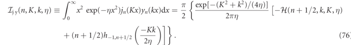
The analytic result for this integral from [36] is given by the rightmost expression in (76). Here h−1,b
denotes an associated Bessel function [68], and  is the following finite-range integral:

Using expansions given by Luke [68] and evaluating the finite integral in (77) by direct numerical integration, the expression (76) may be verified for arbitrary choices of the parameters K, k and η.
The asymptotic treatment given in [36] which takes the limit as η → 0 is lengthy and complicated. However, it yields a simple result, which is in keeping with the well-known result from Watson [48]:

where  and
and  are cylinder functions of integer or real order μ. For the integral (76) we need to take
  and
and  . The expression (78) is used (with a minus sign) to give the contribution from the lower limit to the integral (76). In the case chosen, the asymptotics show that the contribution from the upper limit (infinity) is precisely zero. (For other cases, like the integrals
  and
and  , there is a delta function contribution which comes from the upper limit; this arises if the asymptotic expansion of the integrand in expressions like (76) with η = 0 as x → ∞ contain a constant term in addition to terms oscillating around zero.) The result is in this case:

We now give an example of the effectiveness of the Gaussian 'killing' function technique for the integral (76): see figure 11. Even with a Gaussian with η only equal to 0.01, the divergent integrand is replaced by one which can be integrated accurately. The numerical integration of the Gaussian form with η = 0.01 gives 0.016 4787 − 0.013 8487i, for integration with upper limit 80 or beyond. The analytic value for the integral (79) is 0.016 3332 − 0.013 5188i. For η = 0.005, the numerical integral gives 0.016 4062 − 0.013 6812i, slightly closer to the exact answer, while for η = 0.001, the numerical integration in Mathematica fails.

Figure 11. The effect of a Gaussian 'killing' function on  : n = 1, k = 1.37, K = 2.96 + 0.457i. At left: without the Gaussian factor, the integrand (red: real part; green: imaginary part) diverges strongly; at right: with the Gaussian factor with η = 0.01 the integrand converges to zero for large x.
Download figure:
Standard image High-resolution imageAs a second example, we give in figure 12 plots of the integrand in the following normalization integral:

As η gets smaller, the oscillating real and imaginary parts of the integrand become for larger x concentrated between Gaussian envelopes. The envelopes peak round  , and have a 1/e full width of
  . The peak modulus of the envelope is
 ![$\mathrm{exp}\left\{{[\mathfrak{I}(k)]}^{2}/\eta \right\}$](https://content.cld.iop.org/journals/1367-2630/23/8/083004/revision7/njpac10a6ieqn153.gif) , and the oscillations within the envelope go as
, and the oscillations within the envelope go as ![$\mathrm{exp}[2\text{i}\mathfrak{R}(k)x]$](https://content.cld.iop.org/journals/1367-2630/23/8/083004/revision7/njpac10a6ieqn154.gif) . The oscillatory behavior means that the value of the integral over this peaked region alternates between positive and negative values, and has on average the value zero. To carry out the integral directly for small η becomes increasingly difficult, particularly if
. The oscillatory behavior means that the value of the integral over this peaked region alternates between positive and negative values, and has on average the value zero. To carry out the integral directly for small η becomes increasingly difficult, particularly if  is small in magnitude.

Figure 12. The effect of Gaussian 'killing' functions on  : n = 1,
  (left), k = 4(1.0527 − 0.072 355i) (right). The integrand (red: real part; green: imaginary part) has the Gaussian factors with η = 0.025 (left) and 0.005 (right). The black vertical lines mark the estimates −Im(k)/η for the abscissa corresponding to the peak of the Gaussian envelopes.
Download figure:
Standard image High-resolution imageThe peak value of the envelope increases rapidly as η decreases, while there are more and more canceling positive and negative contributions to the integral. In order to obtain an accurate numerical estimate for the integral, more and more decimal places have to be used in evaluations of the elements of the integrand, if the oscillations are to cancel the diverging peak value.
This means, for calculations with a fixed accuracy (say 10–12 decimal places) there will be a smallest value of η for which the numerical estimate is good. The calculations will get more and more difficult as the ratio  increases. These remarks emphasize the value of the analytic studies [16] which have shown there is a simple explicit and general answer for normalization integrals such as (80).
In region outside the sphere, the specific integrals of the more general exposition of reference [16] that are needed for this work are:
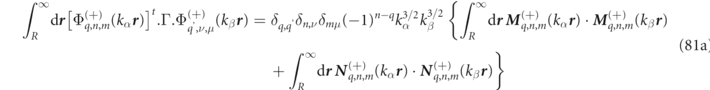
which for α ≠ β are:

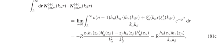
while for β = α one finds:


where zα ≡ kα R, with hn (z) the outgoing spherical Hankel functions, and ξn (z) ≡ zhn (z) the outgoing Ricatti–Hankel functions.
The integrals of the regular partial waves inside a dispersionless homogeneous sphere of arbitrary radius R inside the particle can also be carried out analytically without the need for regularization:
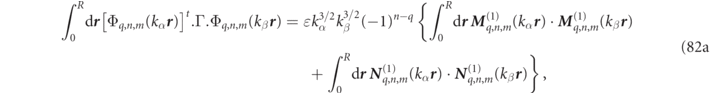
which when α ≠ β, the analytic multipole integrals are:

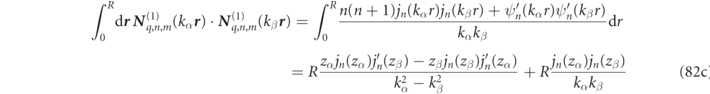
while when β = α, one finds:


where jn are the spherical Bessel functions with ψn (z) ≡ zjn (z). These formulas are particularly useful for spherical scatterers but could also prove useful in non-spherical particles and multiple scattering situations.
Appendix D.: Mie theory
D.1. Multipolar decomposition of fields
Mie theory relies on developing fields in different regions in terms of VPWs, which are homogeneous media electromagnetic wave solutions in an angular momentum eigenstate basis. The excitation field, E e, is the field created by source currents in the absence of the scatterer and it can be developed on the complete basis of 'regular' multipolar fields denoted by a superscripted (1),

where n is the electromagnetic angular momentum quantum number, m an absolute value of the angular momentum projection. The real parameter, E, determines the strength of the incident field. The real-valued multipole wave functions, N q,n,m (k r ) and M q,n,m (k r ), expressed in equation (67) are either of the magnetic, h(q = 0), type or electric, e(q = 1), type (denoted 'even' and 'odd' multipolar types in Bohren and Huffman [46]).
The total field inside a spherical particle can also be developed in terms of regular VPWs provided that position vector in the VPWs is weighted by the field frequency dependent wavenumber inside the sphere, kρω using the notation of equation (11),

Mie theory also involves the 'scattered field' which has its traditional definition as the incident field subtracted from the total field in presence of the scatterer, which can be developed in terms of outgoing VPWs,

which can be viewed as replacing the spherical Bessel functions in the definitions of the regular VPWs by outgoing Hankel functions as shown in equation (68).
D.2. Mie coefficients and cross sections
A consequence of linear response of any scatterer is that if one expresses the scattered and internal fields coefficients, f and s, as infinite dimensional column matrices, then the scattering and internal field coefficients can be expressed in terms of the column matrix of excitation field coefficients via infinite matrices, T and Ω, such that, f = T.e and s = Ω.e. The fact that scattering by spheres does not change the angular momentum, both T and Ω become diagonal matrices for spherically symmetric scatterers and traditional 'Mie' theory provides algebraic expressions for these diagonal elements, henceforth denoted Tq,n and Ωq,n . For the different multipole orders, one has,

where we specified the relation between Tq,n and the time honored Mie coefficients, traditionally denoted an and bn . The 'numerator' and 'denominator' functions in equation (85a) are functions of the angular frequency, ω and particle radius, R are written out explicitly in equations (86) and (87).
Mie theory also provides expressions for the lesser known cn and dn coefficients between the internal field and the incident field decomposition which can be directly expressed in terms of denominator functions,

The 'numerator' and 'denominator' functions in equation (85) are functions of the angular frequency, ω and particle radius, R:


and,


where we have again used z = kR = ωR/c and used the condensed notation of equation (11) for ɛω , μω , and ρω , for the (possibly frequency dependent) constitutive parameters: an inspection of equations (86) and (87) readily shows for non-dispersive media, the, Nq,n and Dq,n reduce to functions of size parameter, z = kR, only.
Cross sections like those plotted in figure 6 are obtained from the Mie coefficients of equation (85a) via well-known relations:


Appendix E.: Resonant state electric field orthogonalization
In the main text, we showed the orthogonality of electric mode RS product integrals for a spherical scatterer when integrating the magnetic field product of the RSs products over all space when α ≠ β. Here we show that RS orthogonality also holds for products of the electric fields of the electric type modes (n.b. the same integrals also arise in magnetic field integration of magnetic type modes). The volume inner product integral inside the sphere for two RSs α and β is zero unless they share the same q, n, m numbers, and in the case where they do share the same q, n, m, their product integral inside the sphere is,


where the rhs of equation (89a) is obtained after analytical integration of the angular variables, while equation (89b) follows from equation (89a) via the analytic result of equation (106) in reference [16]. The final result of equation (89c) exploits the expressions of equation (14a) for γe,n,α and is only true provided that both zα and zβ are RS (size parameter) eigenvalues.
One finishes the electric field inner product by carrying out the volume integral in the region outside the scatterer (i.e. for r > R),


where we used equation (111a) in reference [16] to evaluate the integral in the first line of this equation. Simply adding equations (89c) and (89e) then immediately leads to the orthogonality of the electric type RSs in lossless media when integrating their electric fields over all space,

All the calculations for the magnetic modes when α ≠ β are completely analogous to those of this section and those of section 2.3.1 in the main text up to overall sign factors (which we did not explicit here for sake of clarity).
Appendix F.: Resonant state normalization for Mie theory: dispersive media
F.1. Magnetic mode normalization
The normalization for magnetic (TE) mode fields is found through,

For clarity, the overall magnetic multipole mode sign factor, (−1)n , resulting from the in phase factor in multipole fields (cf equations (9) and (12)) is omitted in this section since it has no effect on normalization and is explicitly included in the response functions expansions of appendix D.
Denoting by, ɛ(ω), the permittivity of the sphere normalized with respect to exterior medium, the contribution to the electric field integral from the volume inside the sphere is,
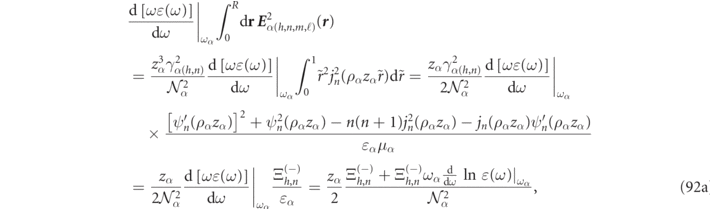
where we used equation (14b) for γα(n,h) and the expression of equation (37c) for  .
.
Denoting by μ(ω), the magnetic permeability of the sphere divided by permeability of the external medium, the magnetic field integral of equation (91) is,
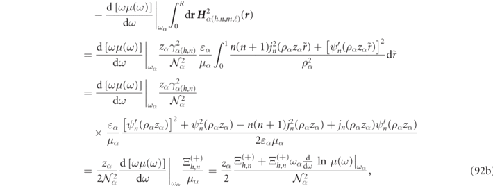
where the  function was again defined in equation (37c).
The exterior integrals are again finite despite their divergent kernels following our regularization approach,

and,

and the sum of the above two integrals yields:

Finally, putting together the results of equations (92a), (92b) and (94) into equation (91), one finds the normalization factor of equation (37a) for magnetic type RSs for spherical scatterers with full temporal dispersion.
F.2. Electric mode normalization
The normalization condition for electric (TM) modes is strictly analogous to those of the magnetic (TE) modes above with:

where the overall electric multipole mode sign factor, (−1)n−1, will be henceforth suppressed for simplicity like we did above for the magnetic modes above.
The E-field integration inside the sphere is,
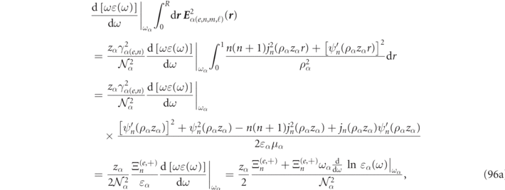
where we used equation (14a) for γe,n,α
and used the definition of equation (37d) for  .
.
The H-field integral inside the sphere is,
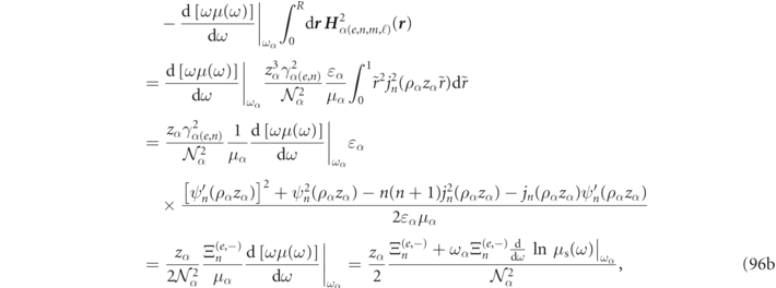
where  is defined in equation (37d).
The integrals outside the sphere are identical to those of equation (93) with the roles of electric and magnetic fields reversed, so we obtain the same result as equation (94) for the field integrals in a region exterior to a sphere of radius R. Inserting the results of equations (94), (96a) and (96b) into equation (95), one finds the normalization factor of equation (37b) for electric type RSs for spherical scatterers with full temporal dispersion.
Appendix G.: Drude models for fitting dispersion relations
Drude models and its extensions can be used to fit experimental measurements like those of Johnson and Christy for silver and gold as shown respectively in figures 13 and 14.

Figure 13. The real (left) and imaginary (right) parts of the complex refractive index of silver as a function of wavelength. Blue: experimental data from Johnson and Christy [69]; red-the Drude model of equation (52a).
Download figure:
Standard image High-resolution image
Figure 14. The real (left) and imaginary (right) parts of the complex refractive index of gold as a function of wavelength. Green: experimental data from Palik; red-the Drude model of equation (52b); blue an alternative Drude model with DC = 5.9752; black—the Drude–Lorentz model of equation (53).
Download figure:
Standard image High-resolution image