Matrix representation of lateral soil movements: scaling and calibrating CE-DYNAM (v2) at a continental level

Fendrich, Arthur Nicolaus; Ciais, Philippe; Lugato, Emanuele; Carozzi, Marco; Guenet, Bertrand; Borrelli, Pasquale; Naipal, Victoria; McGrath, Matthew; Martin, Philippe; Panagos, Panos

doi:https://doi.org/10.5194/gmd-15-7835-2022

Articles | Volume 15, issue 20

https://doi.org/10.5194/gmd-15-7835-2022

Articles | Volume 15, issue 20

Development and technical paper

24 Oct 2022

Development and technical paper |

| 24 Oct 2022

Matrix representation of lateral soil movements: scaling and calibrating CE-DYNAM (v2) at a continental level

Arthur Nicolaus Fendrich, Philippe Ciais, Emanuele Lugato, Marco Carozzi, Bertrand Guenet, Pasquale Borrelli, Victoria Naipal, Matthew McGrath, Philippe Martin, and Panos Panagos

Abstract

Promoting sustainable soil management is a possible option for achieving net-zero greenhouse gas emissions in the future. Several efforts in this area exist, and the application of spatially explicit models to anticipate the effect of possible actions on soils at a regional scale is widespread. Currently, models can simulate the impacts of changes on land cover, land management, and the climate on the soil carbon stocks. However, existing modeling tools do not incorporate the lateral transport and deposition of soil material, carbon, and nutrients caused by soil erosion. The absence of these fluxes may lead to an oversimplified representation of the processes, which hinders, for example, a further understanding of how erosion has been affecting the soil carbon pools and nutrients through time. The sediment transport during deposition and the sediment loss to rivers create dependence among the simulation units, forming a cumulative effect through the territory. If, on the one hand, such a characteristic implies that calculations must be made for large geographic areas corresponding to hydrological units, on the other hand, it also can make models computationally expensive, given that erosion and redeposition processes must be modeled at high resolution and over long timescales. In this sense, the present work has a three-fold objective. First, we provide the development details to represent in matrix form a spatially explicit process-based model coupling sediment, carbon, and erosion, transport, and deposition (ETD) processes of soil material in hillslopes and valley bottoms (i.e., the CE-DYNAM model). Second, we illustrate how the model can be calibrated and validated for Europe, where high-resolution datasets of the factors affecting erosion are available. Third, we presented the results for a depositional site, which is highly affected by incoming lateral fluxes from upstream lands. Our results showed that the benefits brought by the matrix approach to CE-DYNAM enabled the before-precluded possibility of applying it on a continental scale. The calibration and validation procedures indicated (i) a close match between the erosion rates calculated and previous works in the literature at local and national scales, (ii) the physical consistency of the parameters obtained from the data, and (iii) the capacity of the model in predicting sediment discharge to rivers in locations observed and unobserved during its calibration (model efficiency (ME) =0.603, R²=0.666; and ME =0.152, R²=0.438, respectively). The prediction of the carbon dynamics on a depositional site illustrated the model's ability to simulate the nonlinear impact of ETD fluxes on the carbon cycle. We expect that our work advances ETD models' description and facilitates their reproduction and incorporation in land surface models such as ORCHIDEE. We also hope that the patterns obtained in this work can guide future ETD models at a European scale.

Download & links

Article (PDF, 8410 KB)

How to cite

How to cite.

Dates

Received: 28 Apr 2022 – Discussion started: 30 May 2022 – Revised: 13 Sep 2022 – Accepted: 13 Sep 2022 – Published: 24 Oct 2022

1 Introduction

The adoption of more sustainable land management actions constitutes a critical alternative for mitigating climate change and sustaining food production (Roe et al., 2019). Soils constitute a vital carbon (C) pool for the world, storing 1500–2400 Pg of carbon (PgC), more than the atmosphere (589 PgC) and the surface ocean (900 PgC) together, and the way humans interact with soils affects how soils and the atmosphere interact, including the sequestration of carbon (Ciais et al., 2013). It is understood that even minor disturbances to soil pools can have significant impacts on the global C cycle: increases of 4 ‰ in global agricultural stocks, for example, could result in additional C sequestration of 2 to 3 PgC per year, which would contribute significantly to the Paris agreement targets (Guenet et al., 2020; Minasny et al., 2017; Soussana et al., 2019). Alternatives to rapidly increase the content of soil organic matter, and consequently the C sequestration from the atmosphere, include conservation agriculture (e.g., the retention of residues and zero or no-tillage) (Robert, 2001), agroforestry, and afforestation. In the future, however, the projected population growth poses an increasing demand for food, feed, energy, and water, resulting in additional pressures that, if not properly dealt with, can even aggravate the problem (IPCC, 2019). An iconic example is the southeastern Amazon forest, which has long been understood as a C sink, but after decades of deforestation, it is becoming a source of C to the atmosphere (Gatti et al., 2021; Nobre et al., 2016).

One of the possible strategies for evaluating the impacts of different alternatives on the C stocks is the use of numerical models that represent the physical, chemical, and biological processes of the soil–plant–atmosphere system, such as fixation by plants for biomass growth and the respiration by microorganisms (Gettelman and Rood, 2016). Models representing the interaction between soils and the atmospheric system allow the evaluation of how future climate change will impact soils and the opposite relationship. For example, land surface models (LSMs) have allowed studies on different topics, such as assessing the impacts of climate change on crops, habitat, and water availability (Leng and Hall, 2019; Schewe et al., 2019; Hamaoui-Laguel et al., 2015; Bonan and Doney, 2018), evaluating strategies to achieve global environmental targets (Harper et al., 2018; Chang et al., 2021), and forecasting future scenarios of change (Friedlingstein et al., 2006; Friedlingstein, 2015), among others. However, the implementation state of LSMs currently does not cover some relevant processes, such as lateral displacement of nutrients in the soil due to erosion, transport, and deposition (ETD) processes (Quine and van Oost, 2020 a). ETD is argued to affect the carbon cycle dynamically during its occurrence by inducing lateral fluxes of C in the landscape and vertical fluxes between soil layers (Lal, 2003; Lugato et al., 2018), and their absence in LSMs leads to an oversimplified representation of the reality. The modeling complexity, along with the scarcity of empirical data for the phenomenon and the non-standardized nomenclature in the literature, hinders, for example, a further understanding of how erosion has been affecting the soil C pools through time (Lal, 2019; Lugato et al., 2018; Wang et al., 2017; van Oost et al., 2007).

Including the complex ETD-related processes into existing LSMs comes at the cost of increasing the inherent technical complexity of these mechanistic models, such as requiring massive amounts of codes, demanding costly computational resources, and being hard to diagnose thoroughly (Lu et al., 2020). For example, even without ETD-related processes, existing LSMs are so complex with their detailed soil–vegetation–atmosphere feedbacks and multitude of spatial or temporal scales that simulations often must be performed repeatedly for hundreds or thousands of years until a stable condition is reached (Huang et al., 2018). In these cases, calculations can take hundreds of processor hours, and researchers often adopt less detailed or simplified processes to avoid prohibitively slow simulation times (Washington et al., 2008). Practically, such technical problems may hinder their operation by users, who are often individuals with different backgrounds and abilities. Since such problems can have an impact on model testing, validation, and ultimately acceptance by the scientific community, approaches to overcome them have been studied in the recent past. It is, for example, the case of the matrix approach, which consists of representing all carbon fluxes explicitly in matrix form (Luo et al., 2017), which has been reported to increase modularity, facilitate diagnostics, and accelerate spin-up calculations (Lu et al., 2020; Xia et al., 2012; Huang et al., 2017, 2018). For ETD-related processes, the incorporation and development of such approaches are advisable, encouraged, and necessary to enable the complexity of representing the vertical and lateral dynamics of C and sediments on the landscape.

In this paper, we address the problem of scaling the calculations of CE-DYNAM, a hybrid empirical–mechanistic ETD model based on a physical emulator of the carbon cycle in soils (Naipal et al., 2020) on a continental scale. First, we describe the model formulation and show how the matrix approach leads to a sparse linear system, thus making calculations feasible. We expect our mathematical development of CE-DYNAM to facilitate its reproduction and incorporation in LSMs such as ORCHIDEE, DayCent, and others. We then calibrated the model for the study area (i.e., Europe) for the last 150 years using climate forcings with a monthly temporal and a 0.125^∘ spatial resolution (approx. 12.5 km at the Equator) using sediment concentration in rivers from data collected in the field. Comparing the predictions against such observed values is important to evaluate the cumulative effect of all model assumptions, as well as its performance on catchments with different characteristics. Internal and external validation of the results is presented to show their consistency and physical realism. Finally, we exemplify the practical use of CE-DYNAM by presenting the results of the impact of ETD-related processes in a chosen depositional area in the territory. With the model in a matrix form, the calibration, and the pattern obtained at the depositional area, we expect it to form the basis for future large-scale model applications.

2 Materials and methods

2.1 Methodological proposal: the matrix approach

2.1.1 Definitions

The CE-DYNAM model (Naipal et al., 2020) consists of coupling erosion and transport modules to the soil carbon dynamics of any land surface model based on CENTURY (Parton et al., 1983, 1988). Typically, CE-DYNAM uses the revised universal soil loss equation (RUSLE; Renard, 1997), an approach adapted for predicting erosion at a large scale and a coarse spatial resolution, but any other existing option such as the LISEM model (de Roo et al., 1998) could be used. The transport module is a topography-based routing scheme, which uses the altitude (or an approximate digital elevation model) to distribute the sediments and their corresponding organic carbon. The scheme is calibrated with field sediment discharge data to generate realistic values, and the elements are incorporated into the soil organic C dynamics as additional fluxes between pools beyond those initially present in the first-order kinetics of CENTURY (Naipal et al., 2015, 2016). As a remark, CE-DYNAM could be coupled to other carbon models as long as they adopt a first-order kinetics. Some advantages of the coupled approach of CE-DYNAM include the current incorporation of interactions such as the feedback between land use, climate, and erosion (Borrelli et al., 2020; Quine and van Oost, 2020 b), as well as the potential for the future implementation of other components such as soil properties. Figure 1 presents a simplified representation of all fluxes of hillslopes and valley bottom soil pools in CE-DYNAM.

https://gmd.copernicus.org/articles/15/7835/2022/gmd-15-7835-2022-f01

Figure 1A simplified representation of all fluxes in CE-DYNAM. All colors represent the same flux (e.g., the blue arrow represents the input from litter). The example shown corresponds to a specific moment in time, spatial location, plant functional type (PFT), and soil pool. All fluxes with written descriptions are directly affected by the parameters to be calibrated (i.e., γ₁, γ₂, etc.), except for those with an underline. Fluxes whose description is in bold interact with one or more spatial locations, soil pools, or PFTs (right, gray squares).

Download

CE-DYNAM has only been applied at a local scale, such as in the non-alpine region of the Rhine basin (whose total area equals 185 000 km²) (Naipal et al., 2020). However, scaling the model to the continental scale, where the area can be tens of times larger than the application mentioned above, still faces practical implementation difficulties that we address in our current work. A careful evaluation of CE-DYNAM's original implementation allows the identification of three important points. First, from a computational point of view, the original implementation requires the storage of a large amount of data in the computer's memory for its execution, which in practice becomes prohibitive as the geographical area or spatial resolution increases. Second, the original strategy is based on the subdivision of the problem in smaller and adjacent units – generally the sub-basins of a hydrographic basin. This procedure naturally restricts the ability to distribute the solution over different processing units and requires the continuous execution of additional steps of integration of all smaller units, which leads to a significant performance reduction. Third, the equilibrium calculation procedure of the original method consists of the successive iteration of the model, which can be very inefficient (Huang et al., 2018). Alternatives for these problems are more easily perceived when the models' mathematical notation is properly developed and stated.

Thus, to solve the problems above, we first clarify the notation to facilitate the comprehension of details and ensure reproducibility. We do so by adopting a general description and, when necessary, including examples based on ORCHIDEE (Krinner et al., 2005) to illustrate the concepts. The formulation accompanies Table 1, containing all input variables for the model, which helps clarification. The indices in Table 1 refer to five dimensions: the soil pool (c), the spatial location (x, interpreted here as a point of a lattice X representing an area on the surface), the plant functional type (PFT) (p), and the soil depth (d). Besides those dimensions, most variables also evolve in time (t). Some datasets are assumed constant on one or more dimensions during simulations: the geographic area of each cell, for example, varies in space but does not change according to the soil pools, PFTs, soil depth, or time.

(Shangguan et al., 2014)(Poggio et al., 2021)(Poggio et al., 2021)(Poggio et al., 2021)(Farr et al., 2007)Pelletier et al. (2016)(Lehner et al., 2008)

Table 1The external input variables for CE-DYNAM calculation.

Download Print Version | Download XLSX

Mimicking the carbon dynamics of the LSM (in our case, ORCHIDEE) is the most important pillar of CE-DYNAM (Naipal et al., 2020). In general, we can represent the soil carbon pool setting of such LSMs with a set $C_{s} = {c_{1}, c_{2}, \dots, c_{n}}$ . However, in comparison to the LSM in which it is based, CE-DYNAM makes additional assumptions to those described above. One of these assumptions is that the soil carbon pools are divided into two fractions – hillslopes and valley bottoms (i.e., $C_{s} = C_{h} ⋃ C_{v}$ ) – in such a way that the original number of soil carbon pools is twice the number of the LSMs. Such an assumption affects the original calculation depending on the fraction under consideration. For the hillslopes, calculations are modified by the inclusion of an extra flux proportional to the erosion predicted by a chosen model such as the RUSLE. For the valley bottoms, such a flux from hillslopes becomes a new input, and a new lateral dynamics of sediments across the landscape, induced by the terrain slope (s_x) and the flow accumulation ( $1 / w_{x}$ ), is added. These lateral dynamics give rise to most computational challenges in CE-DYNAM since they make the stock in one simulation unit dependent on its neighbors.

Another assumption introduced by CE-DYNAM is a discretization of soil depth, which allows the evaluation of the vertical movement of carbon in layers even when the LSM does not. This is done by first setting m=3 soil layers (that is, surface, middle, and bottom layers) and then defining a set $D = {d_{1}, d_{2}, \dots, d_{m}}$ of soil layers. For example, if one lets d₁=10 cm, d₂=20 cm, and d₃=30 cm, then one is identifying the segment of soil from zero to 10 cm as the surface, the segment from 10 cm to 30 cm as the middle layer, and from 30 to 60 cm as the bottom layer. Throughout this text, we also use the symbol d_k, $k \in {1, 2, \dots, m}$ , to refer to the kth layer. Then, the input from litter to soil pools is distributed along D to calculate the share of input to each soil layer. We describe such a vertical discretization procedure in Sect. 2.1.2, and we denote the vertically discretized version of $I_{x, p_{l}}^{j} (t)$ as ${I^{*}}_{x, p_{l}, d}^{j} (t)$ (Eq. 5).

Because the LSM used in this work is based on CENTURY, carbon pool kinetics will always follow a first-order differential equation. Furthermore, soil carbon is divided into three pools (active, slow, passive) with different turnover rates that vary with temperature, moisture, clay content, and other modifiers (e.g., tillage) (Camino-Serrano et al., 2018). The set of v=15 plant functional types used to represent land cover in the model is denoted here as $P = {p_{1}, p_{2}, \dots, p_{v}}$ . Then, for a fixed layer d_k∈D, a fixed lattice point x∈X, a fixed PFT p_l∈P, a fixed pool c_i∈C_s, and a fixed time t, we let $S_{x, p_{l}, d_{k}}^{i} (t)$ denote its carbon stock.

The formulas for the CE-DYNAM rates are detailed in later sections of the text. However, we can essentially represent how the model evolves in time with Eq. (1). While such a representation omits most model dimensions, it is useful to clarify its dynamics as that of a linear and non-autonomous model (Sierra et al., 2018, Table 1). As we will describe in the following subsections, the coupling of erosion-related processes will always respect this general structure, with the changes consisting of modifications to each of its elements according to the particular case.

\begin{matrix} (1) & \frac{d S}{d t} = I (t) - κ (t) \cdot S (t), \end{matrix}

with S(t) denoting the carbon stock at time t in the pool, I(t) denoting all the pool's input, and κ(t) denoting the output rates. In the equilibrium calculation, the model was iterated several times over the period 1860–1869 until convergence to the pullback attracting trajectory (Sierra et al., 2018). In the transient period, all the elements on the right part of the equation will be known, and the $d S / d t$ calculated will correspond to the increment in carbon stocks at each time step. Essentially, we are interested in evaluating how the carbon stocks S(t) change over the transient period. Through the rest of the text, we frequently refer to Eq. (1) as the basis to form the carbon budget in all cases.

In the matrix approach, we discretize Eq. (1) and represent all fluxes between pools as a linear system. Hypothetically, if no fluxes between pools existed, we would have

\begin{matrix} (2) & S (t + Δ t) = S (t) + I (t) \cdot Δ t - A (t) S (t) \cdot Δ t, \end{matrix}

where $S (t) = {[S_{x, p_{l}, d_{k}}^{i} (t)]}_{\begin{matrix} x \in X \\ l \in [v] \\ k \in [m] \\ i \in [n] \end{matrix}} \in R^{| X | \times v \times m \times n}$ , $I (t) = {[I_{x, p_{l}, d_{k}}^{i} (t)]}_{\begin{matrix} x \in X \\ l \in [v] \\ k \in [m] \\ i \in [n] \end{matrix}} \in R^{| X | \times v \times m \times n}$ , and A(t) is a diagonal matrix with diagonal ${[κ_{x, p_{l}, d_{k}}^{i, i} (t) κ_{x, p_{l}, d_{k}}^{i, i} (t)]}_{\begin{matrix} x \in X \\ l \in [v] \\ k \in [m] \\ i \in [n] \end{matrix}} \in R^{| X | \times v \times m \times n}$ .

However, interactions tend to be complex in more general situations. The following sections show that the routing scheme for valley bottoms creates a dependence between pools of different grid cells, PFTs, and soil layers. While such a property replaces several off-diagonal zero elements of A(t) by non-zero rates, it still preserves the inherently sparse structure of A(t).

Next, we detail how the elements of A(t) and I(t) can be calculated. For simplicity, we exemplify with the first time step of the equilibrium period (t=t₀), but calculations are analogous for all time steps.

2.1.2 Vertical discretization

As mentioned in Sect. 2.1.1, CE-DYNAM vertically discretizes the soil, which has a direct impact on the respiration, erosion, and turnover rates of the original LSM. An exponential increase in the profile depth is assumed, so each soil layer thickness in the discretization profile is calculated from the depth to bedrock, α_x, using two real-valued parameters γ₁ and r:

\begin{matrix} (3) & \begin{aligned} d_{m - k + 1} & = \int_{z = (k - 1) / m}^{z = k / m} α_{x} \cdot \exp (γ_{1} + r \cdot z) d z \\ = \frac{α_{x}}{r} \cdot [\exp (γ_{1} + r \cdot \frac{k}{m}) - \exp (γ_{1} + r \cdot \frac{k - 1}{m})] \\ \forall k = 1, 2, \dots, m . \end{aligned} \end{matrix}

For any choice of γ₁, the parameter r is calculated by constraining the sum of all vertical layers to match the total distance to bedrock. By using the general properties of definite integrals, it is possible to show that it can be analytically calculated with the closed-form solution

\begin{matrix} (4) & r = - \exp (γ_{1}) - W [- \exp (γ_{1} - \exp (γ_{1}))], \end{matrix}

where W(⋅) represents the Lambert W function (see Corless et al., 1996). The example notation of Eqs. (3) and (4) shows an important property of the vertical discretization scheme: the γ₁ parameter depends solely on the soil discretization setting, which is assumed to be identical for all cells in CE-DYNAM. For this reason, there is a single γ₁ value independent of all factors being different (e.g., the spatial location, the PFT, or the variable to be discretized). Besides, this property also means that the vertical discretization is not scale-invariant, and thus the depth scheme must be defined with extra care. In Fig. 2, we show how a possible vertical profile of depth equal to 2 m varies with γ₁: for values closer to zero (left), the profile tends towards a flat one, while for larger values (right), the model tends to calculate a smaller surface layer. The realistic choice of γ₁ must come from the model calibration procedure.

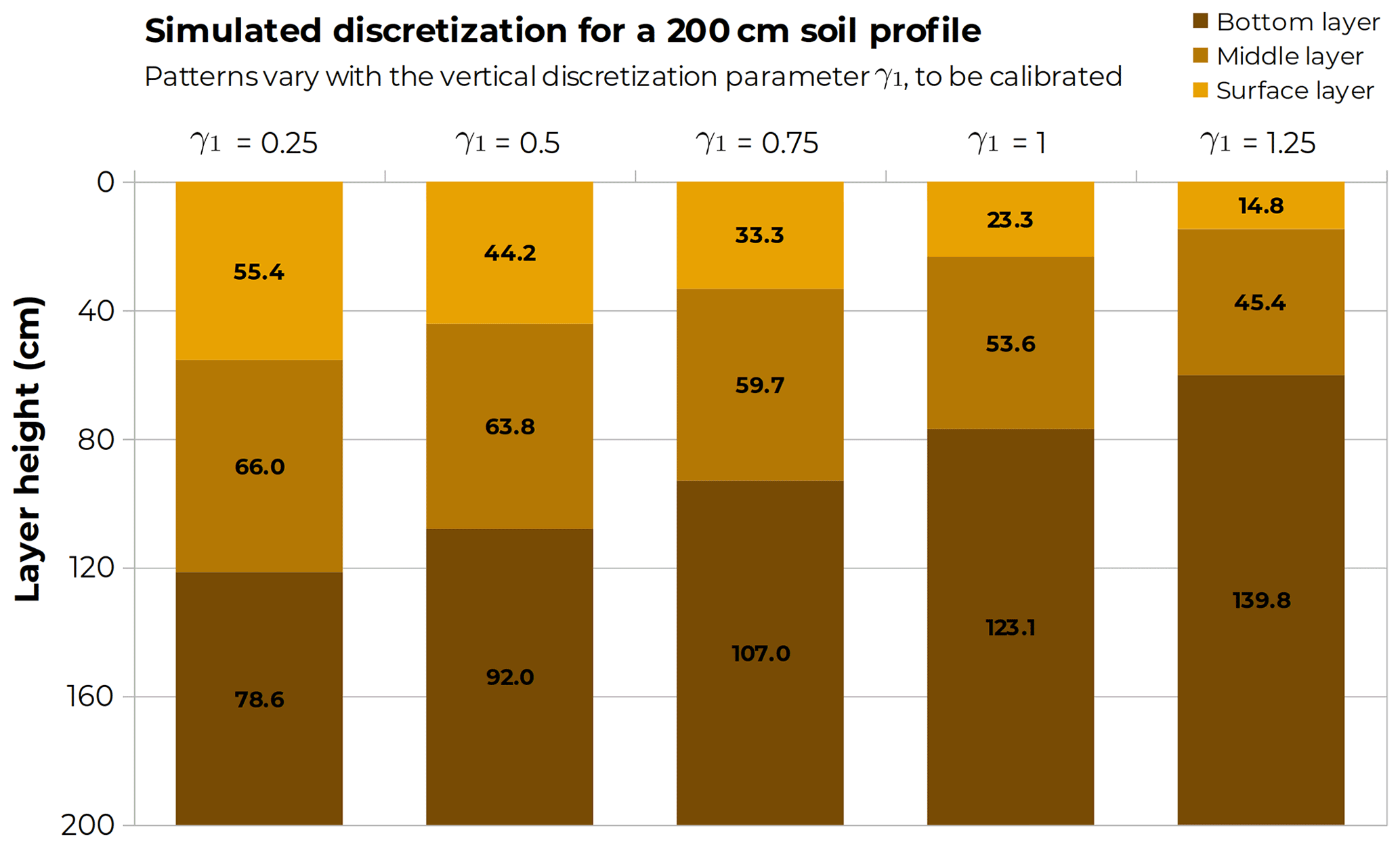
https://gmd.copernicus.org/articles/15/7835/2022/gmd-15-7835-2022-f02

Figure 2Possible options for the vertical discretization parameter in CE-DYNAM. The vertical axis shows the layer heights in centimeters, and the horizontal axis shows some possible γ₁ values.

Download

In the carbon simulation, the input from litter to soil pools is also vertically discretized. This is done by multiplying the original quantity (i.e., $I_{x, p_{l}}^{j} (t)$ ) by the percentage of soil organic carbon in each soil layer (Poggio et al., 2021).

\begin{matrix} (5) & {I^{*}}_{x, p_{l}, d_{k}}^{j} (t) = I_{x, p_{l}}^{j} (t) \cdot \frac{ν_{x, d_{k}}}{\sum_{d} ν_{x, d}} \end{matrix}

For the erosion rates, the vertical discretization is assumed inversely proportional to the mass of soil in each layer. Since not all the carbon eroded in hillslopes goes to valley bottoms, the term is multiplied by a fraction from zero to one, which is assumed to vary with terrain slope and land cover. A different curve is assumed for forests, croplands, and grasslands, and their calibration is made using field observations.

\begin{matrix} (6) & λ_{x, p_{l}, d_{k}} (t) = \overset{RUSLE rate}{\overset{︷}{\frac{e_{x, p_{l}} (t)}{\underset{Total mass of soil}{\underset{︸}{b_{x, d_{k}} \cdot d_{k} \cdot h_{x, p_{l}} \cdot a_{x}}}}}} \cdot \overset{% of erosion that goes to valley bottoms}{\overset{︷}{\frac{1}{1 + \exp (g_{f} (s_{x}))}}}, \end{matrix}

with the multiplication by $h_{x, p_{l}}$ varying for hillslopes and valley bottoms according to their fractions, and g_f(s_x) being the weighted sum of the different smoothing function for forests, croplands, and grasslands multiplied by their corresponding land cover fractions. Although not explicit in the notation, such a function also varies in time, since land cover varies each year.

2.1.3 Fluxes: hillslope soil carbon pools

Bottom soil layer: d_m

We describe the carbon dynamics in hillslopes in terms of three general pools, $c_{1}, c_{2}, c_{3} \in C_{h}$ , which can be interpreted in terms of the active, slow, and passive soil pools of ORCHIDEE. For the deepest soil layer, the rearrangement of Eq. (1) leads to the following equations for c₁, c₂, and c₃, respectively:

\begin{matrix} (7) & \begin{aligned} \frac{d S_{x, p_{l}, d_{m}}^{1} (t_{0})}{d t} & = (\overset{Input: litter pools}{\overset{︷}{\sum_{c_{i} \in C_{l}} {I^{*}}_{x, p_{l}, d_{m}}^{1} (t_{0})}} + \overset{Input: c_{2} pool}{\overset{︷}{κ_{x, p_{l}}^{2, 1} (t_{0}) \cdot S_{x, p_{l}, d_{m}}^{2} (t_{0})}} \\ + \overset{Input: c_{3} pool}{\overset{︷}{κ_{x, p_{l}}^{3, 1} (t_{0}) \cdot S_{x, p_{l}, d_{m}}^{3} (t_{0})}}) \\ - (\overset{Respiration rate}{\overset{︷}{ρ_{x, p_{l}} (t_{0})^{1}}} + \overset{Output: c_{2} pool}{\overset{︷}{κ_{x, p_{l}}^{1, 2} (t_{0})}} + \overset{Output: c_{3} pool}{\overset{︷}{κ_{x, p_{l}}^{1, 3} (t_{0})}} \\ + \overset{Output: erosion B \to T}{\overset{︷}{λ_{x, p_{l}, d_{m}} (t_{0})}}) \cdot \overset{c_{1} stock}{\overset{︷}{S_{x, p_{l}, d_{m}}^{1}}}, \end{aligned} \\ (8) & \begin{aligned} \frac{d S_{x, p_{l}, d_{m}}^{2} (t_{0})}{d t} & = (\sum_{c_{i} \in C_{l}} {I^{*}}_{x, p_{l}, d_{m}}^{2} (t_{0}) + κ_{x, p_{l}}^{1, 2} (t_{0}) \cdot S_{x, p_{l}, d_{m}}^{1} \\ + κ_{x, p_{l}}^{3, 2} (t_{0}) \cdot S_{x, p_{l}, d_{m}}^{3} (t_{0})) \\ - (ρ_{x, p_{l}}^{2} (t_{0}) + κ_{x, p_{l}}^{2, 1} (t_{0}) + κ_{x, p_{l}}^{2, 3} (t_{0}) \\ + λ_{x, p_{l}, d_{m}} (t_{0})) \cdot S_{x, p_{l}, d_{m}}^{2} (t_{0}), \end{aligned} \\ (9) & \begin{aligned} \frac{d S_{x, p_{l}, d_{m}}^{3} (t_{0})}{d t} & = (\sum_{c_{i} \in C_{l}} {I^{*}}_{x, p_{l}, d_{m}}^{3} (t_{0}) + κ_{x, p_{l}}^{1, 3} (t_{0}) \cdot S_{x, p_{l}, d_{m}}^{1} \\ + κ_{x, p_{l}}^{2, 3} (t_{0}) \cdot S_{x, p_{l}, d_{m}}^{2} (t_{0})) \\ - (ρ_{x, p_{l}}^{3} (t_{0}) + κ_{x, p_{l}}^{3, 1} (t_{0}) + κ_{x, p_{l}}^{3, 2} (t_{0}) \\ + λ_{x, p_{l}, d_{m}} (t_{0})) \cdot S_{x, p_{l}, d_{m}}^{3} (t_{0}) . \end{aligned} \end{matrix}

Since CE-DYNAM does not affect litter pools, all quantities in the equations above should be known, except the three hillslope soil carbon pools in the equilibrium calculation. In Eq. (7), we denote as B→T the flux from the bottom layer to the layer above.

Middle and top soil layers

In hillslopes, the structure for middle and top soil layers will be identical to that for bottom layers, except for the B→T loss from the layers below (i.e., the fourth term of Eq. 7), which becomes a new input to the layers above. This results in an additional input equal to $λ_{x, p_{l}, d_{k + 1}} (t_{0}) \cdot S_{x, p_{l}, d_{k + 1}}^{j} (t_{0})$ in the case of pool c_j and depth d_k. One important final remark is that, for the top soil layer, the interpretation of the “Output: erosion B→T” rate becomes “Output: erosion hillslopes → valley bottoms”.

2.1.4 Fluxes: valley bottom soil carbon pools

Preliminary assumptions

In the hillslope soil carbon pools described above, the movement of C was spatially static, which means that all calculations were performed within the same spatial unit (i.e., grid cell). However, the physical definition of valley bottoms extends the movement to other cells, since connected areas exchange sediments and C according to the terrain and land cover configuration. This characteristic is incorporated into the CE-DYNAM model by defining a routing scheme that transports sediments along the landscape.

To represent the lateral transport, a new rate τ_x derived from the sediment residence time is added. Its calculation is performed as

\begin{matrix} (10) & \overset{Sediment rate}{\overset{︷}{τ_{x}}} = \underset{Residence time}{\underset{︸}{\frac{1}{g_{τ} (1 / w_{x})}}}, \end{matrix}

with $g_{τ} (1 / w_{x})$ representing a smoothing function between the sediment residence time and the flow accumulation (i.e., upstream area) to be calibrated from the observations. In this work, we adopted a 3rd degree B-spline to represent all smoothing functions. Besides, the flow accumulation information is also used in the routing scheme to generate an approximated digital elevation model, w_x. Such an approximation is used instead of the original terrain to ensure a hydrologically consistent topography for the lateral movements.

Also, let $P_{x}^{+} (t)$ be the number of non-zero PFTs in cell x at time t and Q(x) be the set of queen neighbors (Fig. 3) (Quinn et al., 1991) of a given cell x formed as

Q (x) = \{y : y - x \in {- 1, 0, 1} \times {- 1, 0, 1}, y \neq x\} .

https://gmd.copernicus.org/articles/15/7835/2022/gmd-15-7835-2022-f03

Figure 3Queen neighbor setting used for the routing scheme. The center cell (red) is x.

Download

With these definitions, the routing scheme for a given cell consists of two elements incorporated into its C balance. First, at the surface depth, d₀, there is loss from the cell to its neighbors, but some definitions are necessary to dictate how the process occurs.

The routing scheme works only within the same carbon pool. For example, the active carbon routed from one cell is added exclusively to the active carbon pool of its neighbor cells.
The C from one PFT in the source cell is transferred equally to all non-zero PFTs of the target cell.
The bare soil PFT (conventionally denoted here by p₀) loses and gains no C on the routing scheme.

The rate of routed C from a PFT p_r of the source cell x to a PFT p_l of the target cell y can then be calculated as

\begin{matrix} (11) & \overset{Lateral transfer rate}{\overset{︷}{θ_{[\underset{Source, Target}{\underset{︸}{x, y}}]}}} = \overset{Indicator function}{\overset{︷}{1_{(w_{y} < w_{x})}}} \cdot \overset{Slope: rise/run}{\overset{︷}{\frac{w_{x} - w_{y}}{| | x - y | |_{2}}}}, \\ (12) & \begin{aligned} \overset{Rate of routed carbon}{\overset{︷}{ζ_{x, p_{r}, y, p_{l}} (t)}} & = \overset{Indicator}{\overset{︷}{1_{(p_{l} \neq p_{0}, p_{r} \neq p_{0})}}} \cdot \overset{Sediment rate}{\overset{︷}{τ_{x}}} \\ \cdot \overset{Local  % of lateral transfer}{\overset{︷}{\frac{θ_{x, y}}{\sum_{y \in Q (x)} θ_{x, y}}}} \cdot \overset{Local % of target PFT}{\overset{︷}{\frac{u_{y, p_{l}} (t)}{\sum_{s = 1}^{v} u_{y, p_{s}} (t)}}}, \end{aligned} \end{matrix}

where the indicator function equals 1 when the condition is met or zero otherwise. Together, Eqs. (11) and (12) result in the important remark: the total loss of C in PFT p_r≠p₀ of the source cell is equal to τ_x times the corresponding C stock at the surface, which varies according to the pool under consideration (for example, $S_{x, p_{r}, d_{0}}^{1} (t_{0})$ for pool c₁). Also, the flux is equal to zero for the remaining case of p_r=p₀, since the bare soil does not participate in the routing scheme. At the surface, the equilibrium value of C stock in one cell and PFT will depend on the equilibrium value of C stock in all the PFTs of all its neighbors. This property of the routing scheme is essential and makes several zero off-diagonal elements be represented as rates from/to different grid cells, PFTs, or soil layers.

Besides, despite affecting more directly the soil surface layer, the routing scheme is also assumed to affect the vertical movement of C described earlier in Sect. 2.1.3 for the case of hillslopes. The same total rate routed from one PFT to the neighbors also moves through the layers, from the bottom to the top (B→T) (i.e., subsoil exposure). In the other way (T→B), the rate received from the neighbors is transmitted vertically from each layer to the layer below (i.e., burial). The only exception is naturally d_m, which has no layers below. Such input rate to p_l can be denoted as $\sum_{y \in Q (x)} \sum_{r = 1}^{v} ζ_{y, p_{r}, x, p_{l}} (t)$ .

Top soil layer: d₀

The equations for the C dynamics in valley bottoms can be obtained by putting the new fluxes along with the other ones from the original LSM. This implicitly assumes that litter input and PFT in valley bottoms are the same as in the standard LSM. Again, we make this section using a general notation of $c_{1}, c_{2}, c_{3} \in C_{h}$ and its respectively correspondent pools $c_{4}, c_{5}, c_{6} \in C_{v}$ . For example, if c₁ is the hillslope soil active carbon pool, then c₄ is the valley bottom soil active carbon pool. Below, we describe the fluxes for PFT p_l of pool c₄ using element-wise notation. For the topsoil layer, d₀, we have input from below but not from above, and we also have inputs from some neighbor cells via the routing scheme and losses for other neighbors for the same reason.

\begin{matrix} (13) & \begin{aligned} \frac{d S_{x, p_{l}, d_{0}}^{4} (t_{0})}{d t} & = (\overset{Input: litter pools}{\overset{︷}{\sum_{c_{i} \in C_{l}} {I^{*}}_{x, p_{l}, d_{0}}^{4} (t_{0})}} + \overset{Input: c_{6} pool}{\overset{︷}{κ_{x, p_{l}}^{6, 4} (t_{0}) \cdot S_{x, p_{l}, d_{0}}^{6} (t_{0})}} \\ + \overset{Input: c_{5} pool}{\overset{︷}{κ_{x, p_{l}}^{5, 4} (t_{0}) \cdot S_{x, p_{l}, d_{0}}^{5} (t_{0})}} \\ + \overset{Input: hillslopes}{\overset{︷}{λ_{x, p_{l}, d_{0}} (t_{0}) \cdot S_{x, p_{l}, d_{0}}^{1} (t_{0})}} + \overset{Input: vertical flow B \to T}{\overset{︷}{\sum_{y \in Q (x)} P_{y}^{+} (t_{0}) \cdot τ_{x} \cdot S_{x, p_{l}, d_{1}}^{4} (t_{0})}} \\ + \overset{Input: routing scheme}{\overset{︷}{\sum_{y \in Q (x)} {\sum_{r = 1}}^{v} ζ_{y, p_{r}, x, p_{l}} (t_{0}) \cdot S_{y, p_{r}, d_{0}}^{4} (t_{0})}}) \\ - (\overset{Respiration rate}{\overset{︷}{ρ_{x, p_{l}}^{4} (t_{0})}} + \overset{Output: c_{5} pool}{\overset{︷}{κ_{x, p_{l}}^{4, 5} (t_{0})}} + \overset{Output: c_{6} pool}{\overset{︷}{κ_{x, p_{l}}^{4, 6} (t_{0})}} \\ + \overset{Output: routing scheme + extra respiration}{\overset{︷}{\sum_{y \in Q (x)} P_{y}^{+} (t_{0}) \cdot τ_{x}}} \\ + \overset{Output: erosion T \to B}{\overset{︷}{λ_{x, p_{l}, d_{0}} (t_{0})}} + \overset{Output: vertical flow T \to B}{\overset{︷}{\sum_{y \in Q (x)} {\sum_{r = 1}}^{v} ζ_{y, p_{r}, x, p_{l}} (t_{0})}}) \\ \cdot \overset{c_{4} stock}{\overset{︷}{S_{x, p_{l}, d_{0}}^{4} (t_{0})}} \end{aligned} \end{matrix}

For the other pools c₅ and c₆, the equations are analogous.

Middle layers

The routing scheme for valley bottoms also affects the middle layers with its vertical components. For having layers above and below, such layers have fluxes in both directions. For a PFT p_l of pool c₄, the equation for d_k, $0 < k < m$ , is

\begin{matrix} (14) & \begin{aligned} \frac{d S_{x, p_{l}, d_{k}}^{4} (t_{0})}{d t} & = (\overset{Input: litter pools}{\overset{︷}{\sum_{c_{i} \in C_{l}} {I^{*}}_{x, p_{l}, d_{k}}^{4} (t_{0})}} + \overset{Input: c_{6} pool}{\overset{︷}{κ_{x, p_{l}}^{6, 4} (t_{0}) \cdot S_{x, p_{l}, d_{k}}^{6} (t_{0})}} \\ + \overset{Input: c_{5} pool}{\overset{︷}{κ_{x, p_{l}}^{5, 4} (t_{0}) \cdot S_{x, p_{l}, d_{k}}^{5} (t_{0})}} \\ + [\overset{Input: erosion T \to B}{\overset{︷}{λ_{x, p_{l}, d_{k - 1}} (t_{0})}} + \overset{Input: vertical flow T \to B}{\overset{︷}{\sum_{y \in Q (x)} {\sum_{r = 1}}^{v} ζ_{y, p_{r}, x, p_{l}} (t_{0})}}] \\ \cdot S_{x, p_{l}, d_{k - 1}}^{4} (t_{0}) + \overset{Input: vertical flow B \to T}{\overset{︷}{\sum_{y \in Q (x)} P_{y}^{+} (t_{0}) \cdot τ_{x} \cdot S_{x, p_{l}, d_{k + 1}}^{4} (t_{0})}}) \\ - (\overset{Respiration rate}{\overset{︷}{ρ_{x, p_{l}}^{4} (t_{0})}} + \overset{Output: c_{5} pool}{\overset{︷}{κ_{x, p_{l}}^{4, 5} (t_{0})}} + \overset{Output: c_{6} pool}{\overset{︷}{κ_{x, p_{l}}^{4, 6} (t_{0})}} \\ + \overset{Output: vertical flow T \to B}{\overset{︷}{\sum_{y \in Q (x)} \sum_{r = 1}^{v} ζ_{y, p_{r}, x, p_{l}} (t_{0})}} + \overset{Output: erosion T \to B}{\overset{︷}{λ_{x, p_{l}, d_{k}} (t_{0})}} \\ + \overset{Output: vertical flow B \to T}{\overset{︷}{\sum_{y \in Q (x)} P_{y}^{+} (t_{0}) \cdot τ_{x}}}) \cdot \overset{c_{4} stock}{\overset{︷}{S_{x, p_{l}, d_{k}}^{4} (t_{0})}} . \end{aligned} \end{matrix}

Bottom soil layer: d_m

Finally, for the bottom soil layer, the equation is identical to Eq. (14), the exception being the inexistence of B→T input or T→B output rates, since there are no bottom layers. In this case, for a given PFT p_l of pool c₄, we have

\begin{matrix} (15) & \begin{aligned} \frac{d S_{x, p_{l}, d_{m}}^{4} (t_{0})}{d t} & = (\overset{Input: litter pools}{\overset{︷}{\sum_{c_{i} \in C_{l}} {I^{*}}_{x, p_{l}, d_{m}}^{4} (t_{0})}} + \overset{Input: c_{6} pool}{\overset{︷}{κ_{x, p_{l}}^{6, 4} (t_{0}) \cdot S_{x, p_{l}, d_{m}}^{6} (t_{0})}} \\ + \overset{Input: c_{5} pool}{\overset{︷}{κ_{x, p_{l}}^{5, 4} (t_{0}) \cdot S_{x, p_{l}, d_{m}}^{5} (t_{0})}} \\ + [\overset{Input: erosion T \to B}{\overset{︷}{λ_{x, p_{l}, d_{m - 1}} (t_{0})}} + \overset{Input: vertical flow T \to B}{\overset{︷}{\sum_{y \in Q (x)} {\sum_{r = 1}}^{v} ζ_{y, p_{r}, x, p_{l}} (t_{0})}}] \\ \cdot S_{x, p_{l}, d_{m - 1}}^{4} (t_{0})) \\ - (\overset{Respiration rate}{\overset{︷}{ρ_{x, p_{l}}^{4} (t_{0})}} + \overset{Output: c_{5} pool}{\overset{︷}{κ_{x, p_{l}}^{4, 5} (t_{0})}} + \overset{Output: c_{6} pool}{\overset{︷}{κ_{x, p_{l}}^{4, 6} (t_{0})}} \\ + \overset{Output: vertical flow B \to T}{\overset{︷}{\sum_{y \in Q (x)} P_{y}^{+} (t_{0}) \cdot τ_{x}}}) \cdot \overset{c_{4} stock}{\overset{︷}{S_{x, p_{l}, d_{m}}^{4} (t_{0})}} . \end{aligned} \end{matrix}

2.2 Study area

In this work, the study area comprises the European Union member states (EU27), plus Switzerland, the United Kingdom, and the Balkan states (i.e., Albania, Bosnia and Herzegovina, Kosovo, Montenegro, North Macedonia, and Serbia). The EU27 is a political and economic block of 27 countries, covering 410×10⁶ ha – larger than the seventh-largest country in the world (India) – and 447 million inhabitants. Switzerland, the United Kingdom, and the Balkan states were included for being spatially adjacent territories. The food and farming sector of the EU27 used 156.7×10⁶ ha of land (i.e., 38.2 % of the total area) for agricultural production in 2016 and currently provides nearly 40 million jobs (i.e., 9.75 % of the total population) (Statistical Office of the European Union, 2020; European Commission, 2021 b).

The EU27 has been promoting changes to shift its agriculture towards more sustainable practices. In 2019, for example, the European Commission proposed the European Green Deal, a growth strategy for the continent that proposes environmental targets, including climate neutrality by 2050. Some of the targets include increasing the share of organic farming from 8.5 % of the total agricultural land to 25 % by 2030 and increasing tree cover by planting 3 billion additional trees also by 2030 (European Commission, 2021 a). Such actions come as an anticipated response to projections of future environmental conditions. For example, the projected patterns of rainfall erosivity for the future indicate an increase in 81 % of the European territory by 2050 (Panagos et al., 2017), which will consequently affect soils, a very relevant natural resource for the achievement of the European Green Deal's goals (Montanarella and Panagos, 2021).

2.2.1 Input data: LSM emulator and erosion rates

The first step to running CE-DYNAM is to build a standalone version of the soil carbon dynamics of an existing LSM, i.e., an emulator. Such a procedure is done by carefully analyzing and modifying the source code of the original LSM to allow the export of all necessary variables for reproducing calculations externally. In this work, we ran ORCHIDEE, a process-based model that simulates vegetation, energy, water, and carbon fluxes (Krinner et al., 2005), with the following settings: (i) version: ORCHIDEE 2.2; (ii) time step and range: daily, from 1 January 1860 to 31 December 2018; (iii) climate: monthly forcings at a 0.125^∘ spatial resolution from the VERIFY project (see https://verify.lsce.ipsl.fr/index.php/presentation, last access: 6 October 2022); (iv) land cover: annual forcing – derived from the ESA CCI Land Cover dataset (European Spatial Agency, 2021; LSCE, 2021).

For the calculation of erosion rates, we applied the well-known revised universal soil loss equation (RUSLE) model, using the values recently developed by the European Commission specifically for our study area (Panagos et al., 2015 e). For a given year (y) and month (m), the monthly erosion rate (E) (in t (ha yr⁻¹ PFT⁻¹)⁻¹) was calculated as

\begin{matrix} (16) & E (y, m) = R (y, m) \cdot K \cdot C (y) \cdot LS \cdot P, \end{matrix}

with R(y,m) being the rainfall erosivity factor¹ (in MJ mm ha⁻¹ h⁻¹ yr⁻¹), K being the soil erodibility factor² (in t ha h ha⁻¹ MJ⁻¹ mm⁻¹), C(y) being the dimensionless land cover and management factor³, LS being the dimensionless slope length and steepness factor⁴, and P being the dimensionless support practice factor⁵. When collapsing the PFT dimension for the calculation of annual or monthly averages, E(y,m) was multiplied by the corresponding land cover fraction p_i for PFT i (Table 1). All the data were aligned and processed on a 0.125^∘ grid.

As seen in Eq. (16), factors K, LS, and P were assumed constant for the whole period 1860–2018, while R(y,m) varies per month, and C(y) varies annually. The source of K is the extrapolated version of Panagos et al. (2014) including stoniness, LS comes from the completely harmonized version of Panagos et al. (2015 b) for the whole study area, and P comes from the database provided by Panagos et al. (2015 d). The first and the second factors cover the whole study area originally, but the third does not, so an additional assumption was added: in places where P was not available (i.e., Switzerland and the Balkan states), it was assumed to be equal to 1. According to the authors mentioned above, K and P were derived from the LUCAS field survey carried out in 2009 and 2012, respectively.

For C, we used the spatial dataset of Panagos et al. (2015 c), but an additional procedure was made to minimize the differences arising from the mismatch in the land cover class definitions and spatial resolution. Such a procedure consisted of fitting a linear regression model to the upscaled version of the original C factor using the target land cover classes as explanatory variables (i.e., $C = \sum_{i} β_{i} {\overline{p}}_{i} + ϵ, ϵ \sim N (0, σ^{2})$ ). An intercept term was intentionally not added to the linear regression, and $\overline{p_{i}}$ is the average land cover from the period 2010–2018, approximately the period of data collection of Panagos et al. (2015 c).

The rainfall erosivity also demanded an extra processing step. The main source for calculations was the monthly erosivity derived and provided by Ballabio et al. (2017). To extrapolate for the past, we assumed a constant erosivity density for the whole simulation period, 1860–2018. That was made by calculating

R (y, m) = r (y, m) \cdot \frac{R^{*} (m)}{\overline{r} (m)},

with R^*(m) being the original monthly erosivity dataset upscaled to a 0.125^∘ spatial resolution, $\overline{r} (m)$ being the average monthly precipitation of the period 2010–2018 (roughly the same data collection period of Ballabio et al., 2017), and r(y,m) being the monthly precipitation for the month m of year y.

2.2.2 Calibration and validation

Calibration

Calibrating CE-DYNAM means ensuring that the values predicted by the routing scheme introduced are realistic and consistent with field observations. To do so, we made an exact copy of the model described in Sect. 2.1.3 and 2.1.4 but replaced the carbon quantities with sediment quantities. Then, we used as field data the information of total suspended solids and river discharge from the GEMStat database (United Nations Environment Programme, 2018) for the whole of Europe. We adopted a squared error cost function between the model predictions and the observations. Because the calculation of analytical derivatives of the cost function with respect to the parameters is hard in our case, minimization was performed using the NEWUOA solver (Powell, 2006, 2008) with early stopping to prevent overfitting.

Like most optimization methods, NEWUOA requires several evaluations of the cost function, which is computationally expensive in our case. For this reason, we calibrated the model using annual averages instead of monthly inputs to accelerate calculations. We also pre-processed our observations by first aggregating annually the total of 10 552 instantaneous observations available, which resulted in 391 annual median values for 40 rainfall stations distributed across Europe from 1979 to 2003. Then, we calculated the 5-year moving averages of the median annual values to simultaneously smooth extreme values from floods that are not modeled in CE-DYNAM and remove stations with a few observations. The final dataset contained 241 observations at 30 stations, whose contributing areas covered nearly one-fourth (23.34 %) of the study area. For each set of parameters, we calculated the predicted sediment stock in the river fraction of the cell (from variable l_x, see Table 1), and the objective function adopted was the squared error between this quantity and the product between the total suspended sediments observed and the water volume in a day (derived from the instantaneous discharge). As in similar works such as Borrelli et al. (2018), the model was assessed using the Nash–Sutcliffe model efficiency (ME) coefficient (Nash and Sutcliffe, 1970) and the coefficient of determination (R²) as defined by Everitt and Skrondal (2010).

Validation

The hillslope erosion rates were externally validated by comparing our estimates with some field observations and modeled values in the literature. We used the compilation of observations by Cerdan et al. (2010) in two ways: (i) we aggregated our and their land cover classes into four common categories (i.e., croplands, grasslands, forest, and bare soil) and compared the distribution of our calculations with their reported point estimates; and (ii) we compared our country averages with their extrapolated calculations for the whole of Europe. We also compared our erosion values to the compilation of local-scale field observations from different sources reported by Panagos et al. (2020) and modeled country averages of Panagos et al. (2015 e) to evaluate the model behavior at a local and regional scale, respectively.

The calibration of the lateral movements on the model was validated both internally and externally. The model's internal consistency was checked by comparing the physical quantities obtained empirically by the calibration procedure with the results previously obtained in the literature. We checked the model's ability to predict the sediment concentrations in places unobserved during the calibration process. For this purpose, the 30 rainfall stations of the final dataset were divided between 24 stations for calibration – i.e., 80 % observed by the model – and 6 stations for validation – i.e., 20 % unobserved by the model.

2.3 Simulations

In order to evaluate the behavior of CE-DYNAM under different scenarios, two simulations were made after model calibration. In Simulation #1 (S1), all ETD-related processes are considered. In Simulation #2 (S2), no ETD-related processes are added to the original LSM fluxes. In this case, the original model is only affected by the vertical discretization of fluxes and the division of soil carbon pools into hillslopes and valley bottom soil carbon pools. With such assumptions, the summation of all the results for soil layers of S2 recovers the original LSM results. In both cases, simulations were run from 1 January 1860 to 31 December 2018.

3 Results and discussion

3.1 LSM emulator and erosion rates

The main result for the LSM emulator is presented in Fig. 4: a comparison of the true values of ORCHIDEE against the predicted ones from the emulator with ETD not enabled. The simulation was made in one random grid cell representative of the model behaviors over the entire studied region. A slight mismatch between original and predicted values exists at early time steps, but as expected, values tend to a nearly identical curve after a few time steps, indicating the adequacy of the emulator to replace the full LSM for erosion calculations with CE-DYNAM. In general, the adoption of an emulator has advantages and disadvantages for CE-DYNAM compared to its implementation directly on an LSM. On the one hand, one can list its simplicity, agility, and flexibility as an advantage to be easily modified for the inclusion of new dynamics, such as the ETD fluxes in the present research or for other LSMs. It could be noted at this point that practically all existing soil carbon model implementations can be represented in a linear form, and therefore, the matrix approach could be applicable and CE-DYNAM coupled (Huang et al., 2018). In fact, Sierra and Müller (2015) and Metzler et al. (2020) demonstrate how the approach could be used even for more complex nonlinear models. On the other hand, the use of a standalone version of the LSM allows the processes to be represented only in a simplified way. In the present work, for example, respiration rates and litter input are always assumed to be identical to those simulated by LSM, whereas the literature suggests that, in fact, these should also be affected by ETD fluxes (Olson et al., 2016). Such a limitation also exists for other important interactions affecting the fate of transported carbon that cannot be properly incorporated into the emulator, such as variation in soil moisture and temperature, as well as in organic matter quality and soil fractions (Lal, 2003).

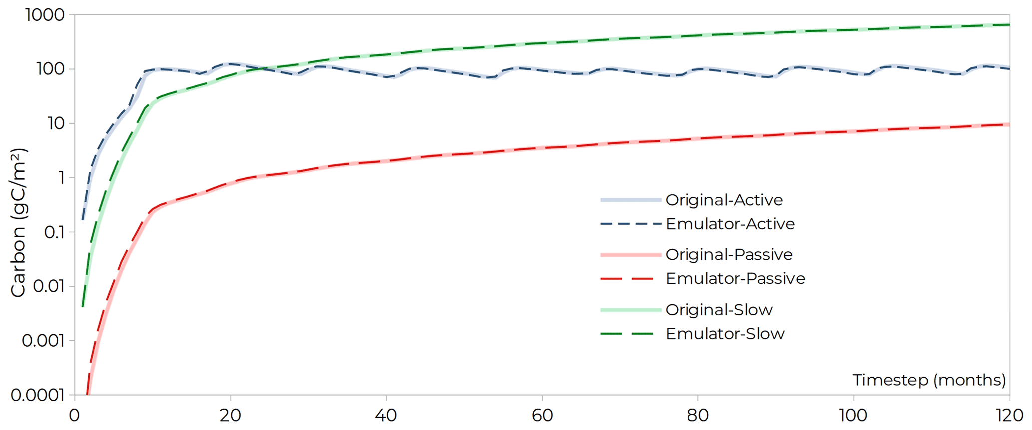
https://gmd.copernicus.org/articles/15/7835/2022/gmd-15-7835-2022-f04

Figure 4Comparison between the results of the original LSM (i.e., ORCHIDEE, continuous lines) and the results of the emulator constructed for the present work (dashed lines), for 10 years of pool initializations. ORCHIDEE does not have a hillslope–valley bottom differentiation of pools, while the line for the emulator corresponds to their sum. Ideally, the emulator would be a perfect standalone version of the LSM.

Download

For the erosion rates, Figs. 5 and 6 present the historical spatiotemporal variability reconstructed. On the top subfigure of Fig. 5, the absolute erosion rates in 1860 are shown on the left, while the maps for 1910, 1960, and 2010 represent the variation with respect to 1860. It can be seen that the annual variations do not follow a linear pattern through time, thus affecting erosion calculations unequally. A decrease in erosion rates from 1860 to 2010 can be noted in Central Europe, and a strong pattern on countries' borders follows from the assumptions of the reconstructed land cover database used (LSCE, 2021). Although partially, this result is related to those reported by Bork and Lang (2003) and Dotterweich (2008), who in historical reconstructions in Germany and Central Europe found peaks in erosion rates in the second half of the 18th century, a period for which there is documentary evidence of extreme rainfall events, and in the early 19th century. In Fig. 5, the 1860 erosion map also shows points in four different locations (i.e., P1, P2, P3, and P4, plus the whole study area (WSA)). Within a year, the monthly variations in erosion rates are due solely to changes in the rainfall and the erosivity factor, and as seen in the bottom graph of Fig. 5, the pattern of such changes also varies nonlinearly in space and may differ from the average pattern of the study area. Additionally, Fig. 6 shows the annual average erosion rates, calculated as 2.96 t ha⁻¹ for 2018. Such a value is higher than the 2.46 t ha⁻¹ reported by Panagos et al. (2015 e), which can be justified by the different spatial resolution, land cover database, and study area, since, in our case, we include Switzerland and the Balkan states, which have erosion rates that are relatively higher compared to their neighbors (Fig. 5, top left). Fig. 6 also shows the average effect of the two time-varying factors adopted for RUSLE calculation, i.e., the R and the C factors of Eq. (16). Two distinct patterns of variation can be seen through time, with the R factor having a higher annual variability and the C factor being less abrupt, except for the evident breaks during the two World Wars. The R factor shows a cyclic pattern from 1860 to 1901 due to the recycling of (i.e., repetition of climate) forcings adopted by ORCHIDEE for this period. The calculations also indicate an overall increase in erosion rates from 1860 to 1960 due mainly to land cover changes and a peak in rainfall erosivity, followed by an overall decrease from 1960 to 2018. Despite such a pattern in the nearer past, the literature indicates a tipping point in the present. Future projections from Panagos et al. (2021) indicate that water erosion in Europe is expected to increase between 13 % and 22.5 % by 2050, and Borrelli et al. (2020) estimate an increase in 2015 water erosion rates of 33 % to 66 % by 2070 worldwide. Under these scenarios, future values could be even higher than the past values calculated and shown in Fig. 6.

https://gmd.copernicus.org/articles/15/7835/2022/gmd-15-7835-2022-f05

Figure 5Annual erosion rates calculated in this work. In the top subfigure, the top-left map shows the erosion rates for 1860 and four points (P1, P2, P3, and P4), while the top-right, bottom-left, and bottom-right maps show the anomalies for 1910, 1960, and 2010, respectively. The bottom subfigure shows the changes in erosion rates due to variations in the monthly rainfall and erosivity for P1, P2, P3, P4, and the whole study area (WSA) within the same year, 1860.

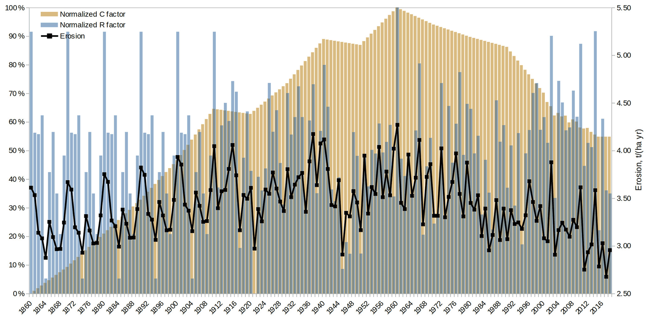
https://gmd.copernicus.org/articles/15/7835/2022/gmd-15-7835-2022-f06

Figure 6The average impact of the reconstructed R and C factors on the erosion rates for the period 1860–2018.

Download

Also for the erosion rates, the annual country averages were compared against values reported in the literature. The results of Fig. 7 (left) show a positive agreement between all databases considered, as highlighted by the positive slope of the robust linear models fitted to the data. The steepness of curves suggests that the model's ability to reproduce the continent-scale patterns is higher than local-scale predictions, which can be interpreted as a consequence of the model's relatively coarse resolution to represent local-scale hydrology. On the right part of Fig. 7, the comparison per land cover class shows a close match for croplands and bare soil, the highest rates in our model. On the other hand, our model tends to underestimate erosion in forests and grasslands compared to the external sources, with our values lying on the lower tail of the distribution of Panagos et al. (2015 e) and Cerdan et al. (2010).

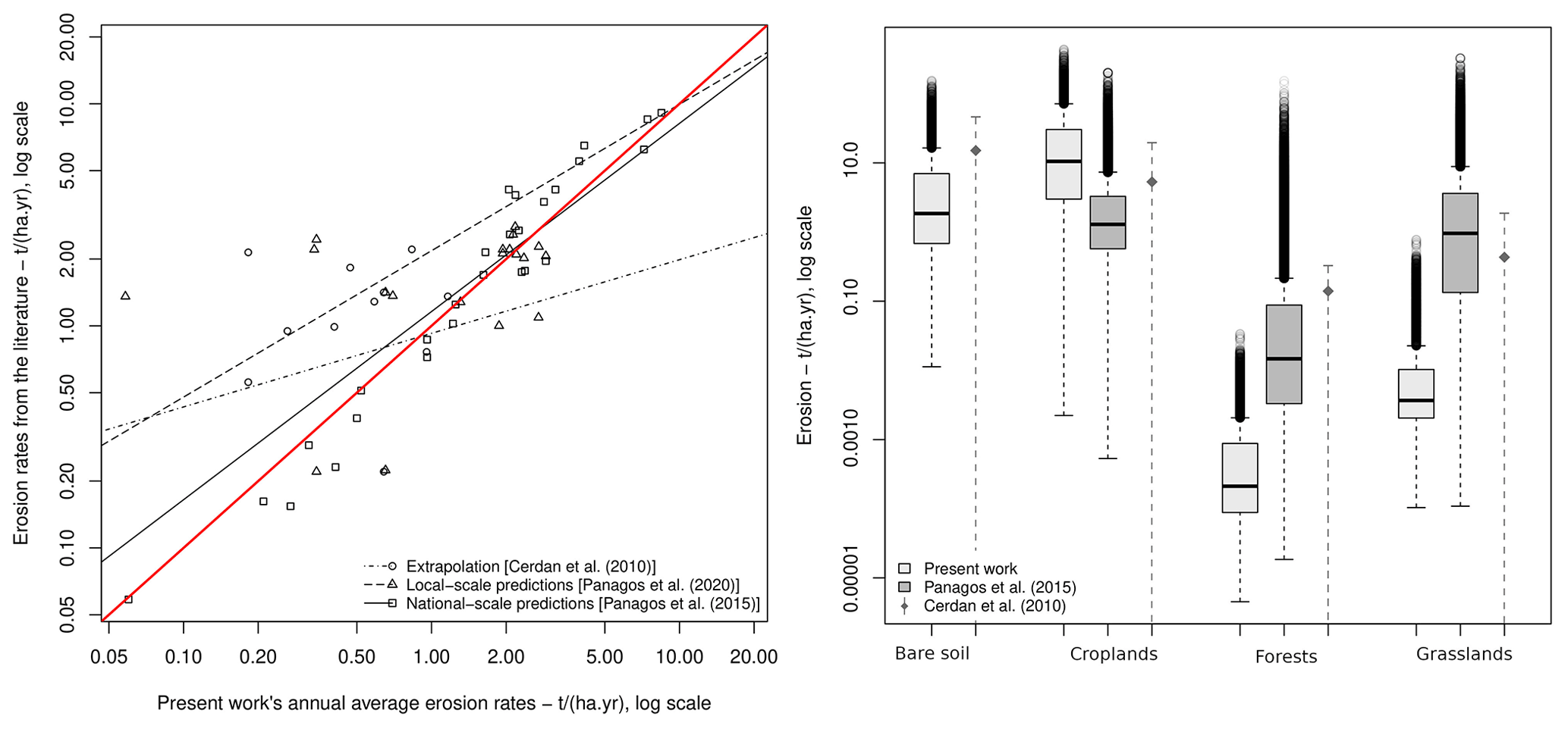
https://gmd.copernicus.org/articles/15/7835/2022/gmd-15-7835-2022-f07

Figure 7Comparison between the average erosion rates calculated by external sources versus the values calculated in our work, along with an identity line (left), and the comparison of the distribution of erosion rates per land cover (right). In the right plot, the values for our work are the average for the period 1970–2018, and the values for Cerdan et al. (2010) are the reported mean ± standard deviation.

3.2 Model calibration

The NEWUOA algorithm performed several hundred function evaluations until stopping. Using averaged annual instead of monthly forcings and performing the calculation only for the catchments areas of stations, each evaluation took around 6 min of processing time. The vertical discretization parameter obtained was γ₁=0.1, approximately the left pattern from Fig. 2. Calibration also indicated that the input of sediments from hillslopes into valley bottoms varies from 0.4 % to 11.8 % in croplands, from 4.9 % to 10.9 % in forests, and from 0.3 % to 3.8 % in grasslands (Fig. 8a). These values can be interpreted in several ways. First, the absolute magnitude of the values is relatively small, following what was suggested by Hoffmann et al. (2013 a), with the maximum values being comparable to the 15 % of on-site erosion reaching riverine systems presented by Borrelli et al. (2018) for the same study area. However, the direct comparison of these values should be read with caution because of the large methodological differences between works. For example, the authors defined the rivers explicitly and used a higher spatial resolution for a single moment in time, characteristics that contrast with those of CE-DYNAM (Naipal et al., 2020). Furthermore, despite the similar interpretation, the quantities compared may themselves differ between the models adopted (Rompaey et al., 2001). Second, regarding the shape of the curves, there is an increasing relation in parameter g_f as a function of slope for forests and croplands but a decreasing relation for grasslands. The increase in two of the three land-use classes can be readily explained by the important effect of gravity on sediment transport (Bridge, 2003; Huggett, 2017), while its generally low range of values can partially explain the unexpected decrease in grasslands compared to that of forests and croplands. Third, with respect to the ordering of the curves, two patterns are observed. In flat areas, with a slope less than 1.5^∘, the pattern is forests having higher transport than grasslands, followed by croplands. In steeper areas, with slopes above 1.5^∘, there is a rapid change in the ordering, leading to a situation where croplands generally have higher sediment transport than forests and grasslands. The low influence of this region on sediment production can explain the non-intuitive relationship between the classes. For example, areas with slopes less than 1.5^∘ were responsible for only 5.43 % of Europe's total erosion in 2018, with the remaining 94.57 % occurring in the steeper areas. Therefore, it is reasonable to expect that the steeper areas will be better represented in the model. Thus, the later pattern of Fig. 8 can be explained by the lower cohesive properties of the less vegetated covers relative to the more vegetated ones, consequently offering less resistance to water and sediment flow (Osterkamp et al., 2011; Hoffmann et al., 2013 a; Huggett, 2017). Figure 8b, also shows the sediment residence time, which was estimated to vary from 0.5 years (180 d) to 24.5 years, indicating that sediment retention increases with watershed size, in agreement with that described by Hoffmann et al. (2013 b).

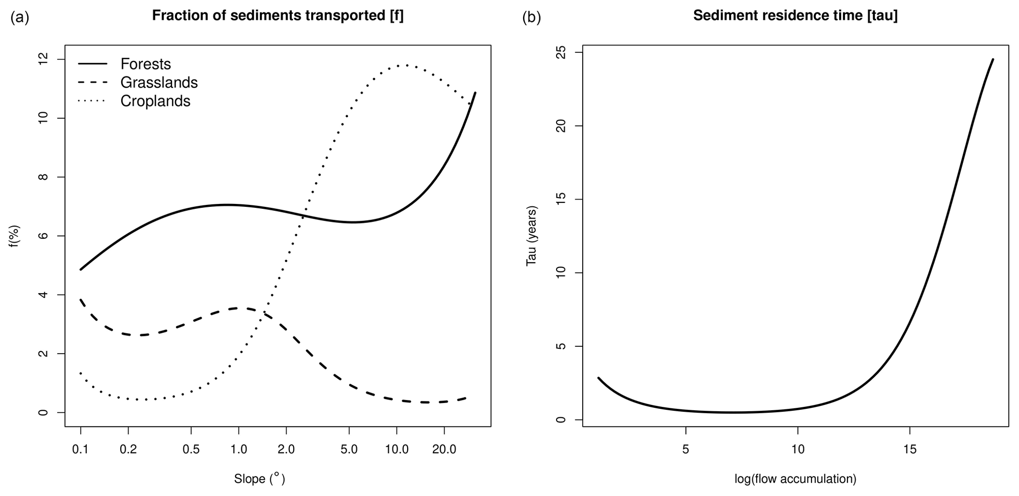
https://gmd.copernicus.org/articles/15/7835/2022/gmd-15-7835-2022-f08

Figure 8Results from the calibration procedure: the fraction of sediments that go from hillslopes to valley bottoms (a) and sediment residence time (b).

Download

The validation for the best set of parameters is summarized in Fig. 9, which shows a plot of actual against predicted values (using annual forcings) for the observed and the unobserved locations. In all cases, the prediction value used for this comparison are those from the same year as the observation. The red diagonal is a 1:1 line, and each group of dots connected by a line represents a different station. The best set of parameters found yielded ME =0.603 and R²=0.666 for the observed stations and ME =0.152 and R²=0.438 for the unobserved stations. Overall, for the full dataset, the model has ME =0.578 and R²=0.640. The values obtained are relatively high when compared to similar studies. Works such as that of Feng et al. (2010) and Rompaey et al. (2005) in China and Italy, respectively, reported negative ME values, which indicate that sometimes distributed models are unable to represent sediment dynamics, especially when there is high heterogeneity in the data (Rompaey et al., 2005). In Quijano et al. (2016), where the authors studied four adjacent hydrological units at a local scale in Spain, distributed models could represent well the dynamics involved. The overall value obtained for the study region was ME =0.11, while the value calculated individually per hydrological unit ranged from ME $= - 0.11$ to ME =0.49. In what is probably the most similar to our work in terms of the study area, Borrelli et al. (2018) initially considered a total of 24 semi-natural and agricultural basins in Europe, for which they obtained ME =0.38. The result motivated the authors to further remove basins as a fine-tuning of the model calibration used, which led to ME =0.89 for 10 basins. The results from these other studies help us to compare the performance of the model presented in the current work. It can be noted that the present work uses more observations and calibrates the model with time-varying data (i.e., not long-term averages), which requires a more complex model architecture and highlights the robustness of the calibration performed. It is also an important remark that the comparison with other works was only possible after the methodological improvements in the new version of CE-DYNAM compared to that of Naipal et al. (2020): (i) the possibility of calibrating the lateral fluxes using sediment data collected in the field and relatively abundant in the literature (see United Nations Environment Programme, 2018); and (ii) the possibility of performing validation with field data, using the model as a basis for prediction for locations unobserved during its fit.

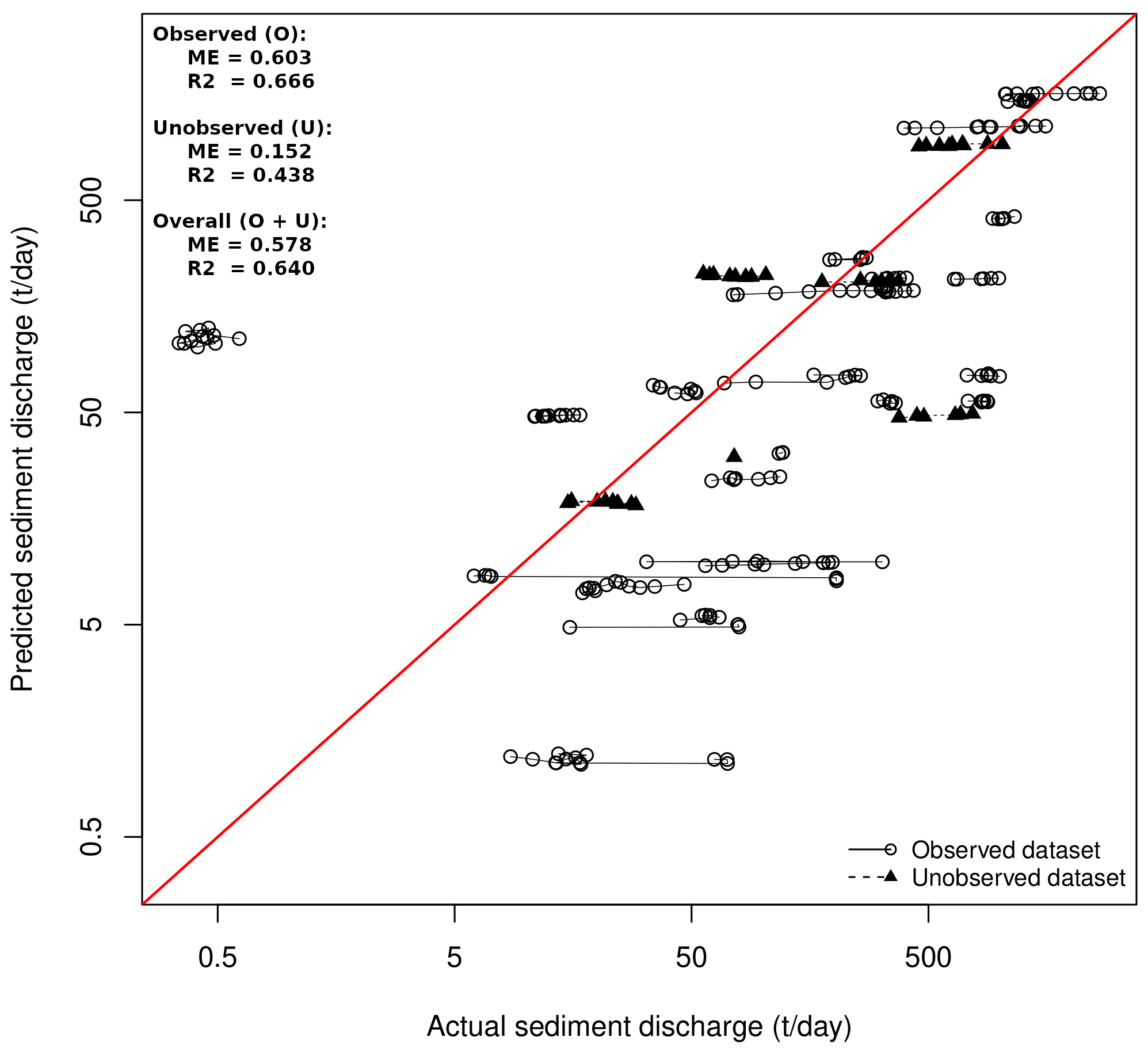
https://gmd.copernicus.org/articles/15/7835/2022/gmd-15-7835-2022-f09

Figure 9Plot of the predicted annual averages against the observed annual sediment discharge values in log scale. Each dot or triangle corresponds to 1 of the 241 observations, and the connected icons correspond to 1 of the 30 different stations of the database. The red line is an identity line.

Download

We also used the same best set of parameters with monthly forcings to quantify how distant the simplified calibration with annual forcings is from the optimal condition. Using monthly forcings for a full calibration remains precluded, since a single function evaluation took almost 1 d to complete. In that experiment, values dropped to ME =0.464 and R²=0.616 for the entire dataset, indicating a relatively small change in predictions compared to the simplification using annual forcings.

3.3 Simulations

In both scenarios, the two A matrices (i.e., one for hillslopes and the other for valley bottom calculations) are square with a size equal to the product between the number of cells, the number of PFTs, the number of soil layers, and the number of soil carbon pools, which for the setting used in the present work equals 1.85×10⁷ rows and columns. In S1, where all fluxes are considered, the average number of non-zero elements on the A matrices of hillslopes and valley bottoms were 7.4×10⁶ and 1.7×10⁷, respectively, corresponding to densities of 21.6 ppb (i.e., 10⁻⁹) and 49.7 ppb. In S2, where fewer fluxes are simulated, the A matrices for hillslopes and valley bottoms contained 5.9×10⁶ and 7.4×10⁶, yielding a density of 17.2 and 21.6 ppb, respectively. Simulations were run on a high-performance computer having 19 Intel(R) Xeon(R) CPU E5-2640 v4 2.40 GHz processors. The number of cores used for calculations varied, as specified next. In both scenarios, the generation of A and B took around 3 to 6 min for each simulation month at the continent scale. After the generation of all matrices, equilibrium calculation took around 10 min on a single core. As a comparison, the calculation for the non-alpine region of the Rhine basin of Naipal et al. (2020) used to take 2 d in seven cores of the same machine. The drastic reduction is a consequence of the matrix approach adopted. While in their work all fluxes had to be recalculated for each month of equilibrium calculation, in our case we just had to precalculate A and B once.

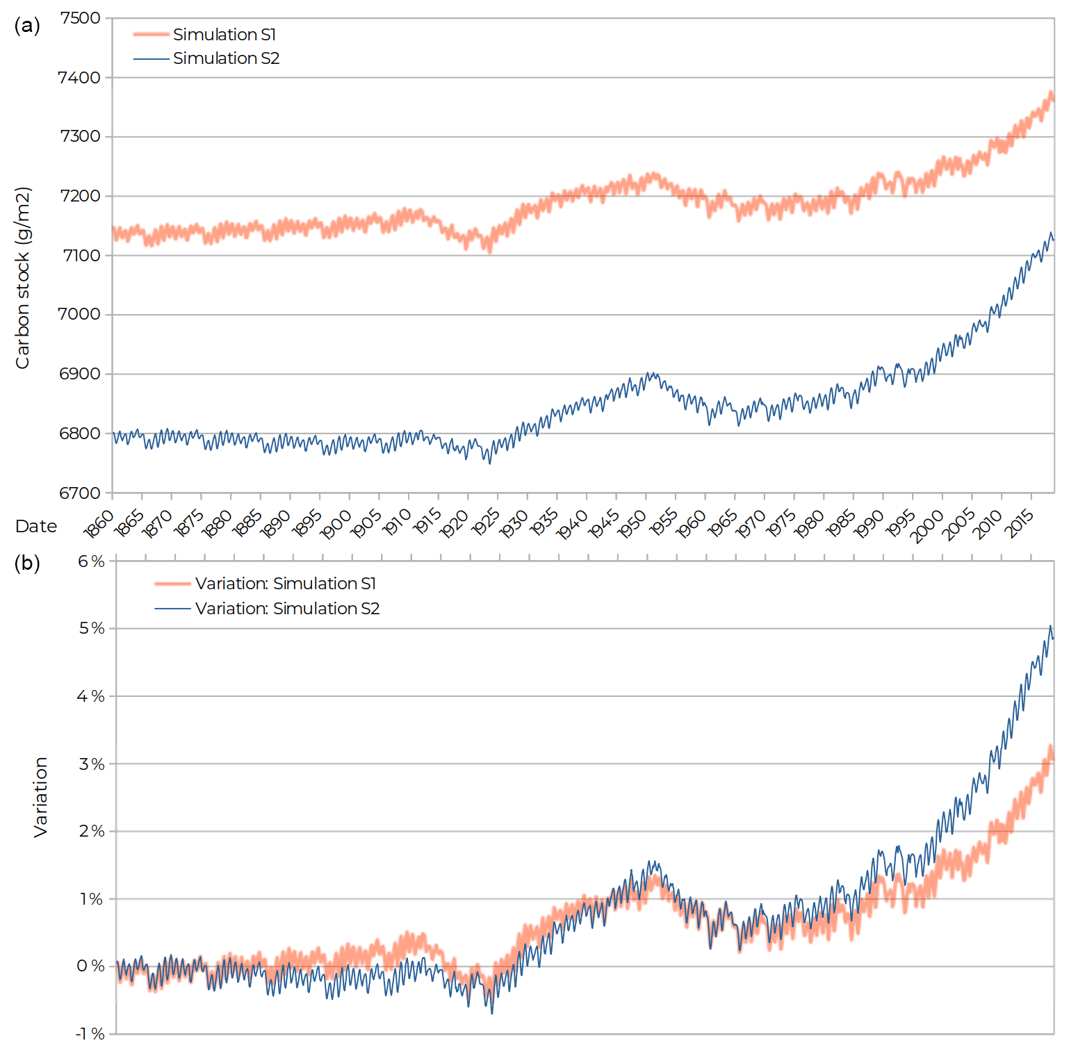
https://gmd.copernicus.org/articles/15/7835/2022/gmd-15-7835-2022-f10

Figure 10Results for the depositional site: absolute values of carbon stock (g m⁻²) (a) and relative difference (b).

Download

The matrix approach brought several benefits for speeding up the model. First, the analytical representation of the model allowed the derivation of first-order approximations for the monthly averages, which are faster to calculate than summing the daily simulations and dividing by the number of days. Second, despite the different settings of S1 and S2, implementation was straightforward thanks to the natural interpretation of each element of A as a flux of carbon from one to another uniquely identified combination carbon pool. Third, the calculation of A and B are independent for each month, which drastically increases the number of possible concurrent execution threads in comparison to the original model of Naipal et al. (2020). These results are similar to those found in the literature. For example, Xia et al. (2012) and Huang et al. (2018) reported reduced processing time and computational cost of the calculations. In our case, it is not possible to compare the processing times as done by Xia et al. (2012) because the previous version of the CE-DYNAM from Naipal et al. (2020) does not support the calculation at a continental scale in a feasible time. In this sense, the very possibility of applying the model at this scale, now allowed because of the matrix approach, is an indicator of such improvements. However, the matrix approach may require changes for applications at even larger scales, such as the global scale. As shown in Eq. (2), the approach simplifies the simulation by representing the variation of fluxes with additions and matrix–vector multiplications. Such operations are typically efficient in the format known as compressed sparse row (CSR) (Bai, 2000; Greathouse and Daga, 2014), which requires the storage of three vectors for its construction. In global-scale problems, it is possible that the amount of memory required for such storage is excessively large, so alternative representations should be explored. A possible solution may come from an analogous problem in the statistical regression literature, where authors seek low-rank representations of models in order to reduce the dimensionality of the problem while still largely preserving the characteristics of the original model (see Wang and Ranalli, 2006 and Wood, 2006, for two examples). However, while procedures that are central for dimensionality reduction problems such as singular value decomposition are well established for dense matrices (Strang, 2016) or even sparse matrices of reasonable size, the problem can be complicated when the dimensions are huge. Therefore, further research and work to search for applicable methods are needed.

The calculation for a depositional site indicates that the additional incoming fluxes from its upstream area due to ETD processes tend to increase the carbon stock at the site from 6800 to 7150 g m⁻² at equilibrium, equivalent to a 5.1 % increase (Fig. 10a). Figure 10b, illustrates the ability of the model to emulate nonlinearities on the impact of ETD fluxes on the carbon cycle. The results are supposed to represent the impacts of the ETD fluxes on the carbon cycle of a depositional area. According to van Oost et al. (2005), Li et al. (2007), and Wang et al. (2015), some expected changes in the dynamics include an increase in the C burial, resulting in an increase in the soil organic carbon, as well as enhanced respiration of the carbon buried with time (Naipal et al., 2020). In fact, in the early period of the curve, from 1860 to approximately 1940, the curve of the S1 simulation is above that of the S2 simulation, indicating that the immediate impact of adding new fluxes to an area is to increase the rates of carbon burial. However, in the final period of the curve, from 1941 to 2018, the variation curve of S1 moves below the S2 curve, indicating a decrease in the lateral input and the rate of carbon burial, as well as a higher respiration by microorganisms due to the carbon previously buried.

Furthermore, to check the mass balance closure, all the fluxes from this depositional area were calculated from 1860 to 2018. On the cell's hillslope fraction, litter input added 25 404.47 gC m⁻², and land cover added 128.71 gC m⁻², of which 25 286.00 gC m⁻² were respired, and 0.39 gC m⁻² were sent to the valley bottoms. On the valley bottom fraction, the inputs were 0.39 gC m⁻² coming from the hillslopes, 722.16 gC m⁻² from upstream lands, and 6039.23 gC m⁻² from litter. Of this, 6764.07 gC m⁻² was respired, and 23.91 gC m⁻² was lost due to land cover change. These values indicate that local erosion at this depositional area is not relevant to the carbon cycle, in contrast to the carbon input from upstream lands, which corresponded to 10.68 % of all the valley bottom fraction inputs.

4 Limitations

Despite the advances presented in this work, there are still limitations that need to be addressed with future modifications. Concerning its structure, incorporating sediment data in CE-DYNAM is only possible by assuming that sediment and carbon follow the same dynamics. While this is convenient for calibration, it might not be realistic, so further work is necessary to improve this important assumption. Besides, the physical representation of the fluxes could be improved. For example, no transformation of C pools during the transport process is represented, such as the breakdown of aggregates. In practice, they could increase the turnover rates of soil organic carbon compared to the simulations we presented.

Regarding the calibration presented here, other limitations concern the spatial resolution and historical reconstructions. First, finding the optimal resolution for CE-DYNAM will always be a problem, since it is halfway between the fine-scale hydrological processes it represents and the coarse resolution of the current climate models. Second, the historical reconstructions presented are highly sensitive to the assumptions adopted and presented. Even though these assumptions are properly evaluated during the calibration and validation process, better results will be possible with better input maps.

Another important limitation refers to the structure of the calibration parameters. The structure presented in this work allows a certain balance between the share of sediments that move from hillslopes to valley bottoms and the sediment residence time so that the optimization may sometimes tend to yield physically unrealistic results. In the present work, this was solved by using multiple starting points, but a better solution in the future should come from the development of the model itself to penalize solutions that do not have a meaningful physical interpretation. Finally, our model also naturally inherits the problems of some necessary assumptions. Even the fundamental assumption that calculations converge to the pullback attracting trajectory in 1860–1869 might not be correct and might affect the results greatly (Sanderman et al., 2017; Dimassi et al., 2018). Analogously, the RUSLE-based approach for erosion modeling is widely criticized but remains the sole alternative for large-scale quantitative applications (Panagos et al., 2016).

5 Conclusions

In this paper, we addressed the challenge of scaling CE-DYNAM, an erosion–transport–deposition model, in a relatively high spatial resolution and long period at the European scale. First, we show how the lateral fluxes of CE-DYNAM can be represented in a matrix form, an alternative that allows the acceleration of the computations performed, making them feasible for large-scale applications. Our work, therefore, enabled the previously precluded possibility of applying CE-DYNAM to large spatial domains or high spatial resolutions. We also improved the model's physical representation of sediment movement to allow for proper calibration and validation procedures using observations of sediment discharge collected in the field. With these changes, the presented model can be readily adapted to other study regions, the main limiting factor being the availability of inputs from external sources. We also describe how the proposed technical solution might not work on an even larger scale (global scale, for example), so further work may be needed to improve the proposed approach, such as the search for the computation of low-rank representations of the model matrices.

Second, a more practical contribution of our work was the calibration of the model for the whole of Europe from field-collected data. Our results show that the patterns obtained are internally consistent and coherent with those previously reported in the literature in similar work. We expect the patterns obtained in this work to serve as a reference for future models for this study region. Since the calibration of the lateral fluxes is done using sediment data, the results form the basis for simulations of the impact of erosion on the carbon cycle and the future incorporation of other nutrients, such as nitrogen and phosphorus, into CE-DYNAM. These works could advance our understanding of the role of ETD processes in nutrient cycles.

Third, we used the calibrated model to predict the movement of carbon at a depositional site, the type of site that tends to be highly affected by incoming lateral fluxes from upstream lands. This simulation evaluated the model's impact on soil carbon pools and showed how the effect of erosion on the carbon cycle could be nonlinear in time. In this sense, this result shows that time-static models can only partially disclose the correct effect of ETD on the carbon cycle.

Code and data availability

The codes are available at https://doi.org/10.5281/zenodo.6553890 (Fendrich, 2022). The dataset used can be made available upon request to the corresponding author, and results of Fig. 5 are available at the European Soil Data Centre (ESDAC). Access to the data used in the paper has been granted to the editor and reviewers during the peer-review process.

Author contributions

ANF, PC, EL, MC, BG, VN, PM, and PP conceived the idea. ANF, PC, EL, MC, BG, PM, and PP conducted the study. PC, PM, and PP were responsible for funding acquisition. All authors contributed to the methodology adopted, to the simulations, to the discussion, and to the writing and editing of this paper.

Competing interests

The contact author has declared that none of the authors has any competing interests.

Disclaimer

Publisher’s note: Copernicus Publications remains neutral with regard to jurisdictional claims in published maps and institutional affiliations.

Acknowledgements

The authors would like to thank Philippe Peylin for granting access to the high-resolution VERIFY forcings, Francis Matthews for the constructive discussions about model calibration, Leonidas Liakos for the European map layouts, Gerd Sparovek for the comments prior to the submission, and Lucas Resende for reviewing the mathematical notation.

Financial support

This research has been supported by the European Commission (grant no. 35403) and by the CLAND project.

Review statement

This paper was edited by Carlos Sierra and reviewed by Yuanyuan Huang and Holger Metzler.

References

Bai, Z.: Templates for the solution of algebraic eigenvalue problems: a practical guide, Society for Industrial and Applied Mathematics (SIAM, 3600 Market Street, Floor 6, Philadelphia, PA 19104, Philadelphia, Pa, ISBN-13 978-0898714715, ISBN-10 0898714710 2000. a

Ballabio, C., Borrelli, P., Spinoni, J., Meusburger, K., Michaelides, S., Beguería, S., Klik, A., Petan, S., Janeček, M., Olsen, P., Aalto, J., Lakatos, M., Rymszewicz, A., Dumitrescu, A., Tadić, M. P., Diodato, N., Kostalova, J., Rousseva, S., Banasik, K., Alewell, C., and Panagos, P.: Mapping monthly rainfall erosivity in Europe, Sci. Total Environ., 579, 1298–1315, https://doi.org/10.1016/j.scitotenv.2016.11.123, 2017. a, b

Bonan, G. B. and Doney, S. C.: Climate, ecosystems, and planetary futures: The challenge to predict life in Earth system models, Science, 359, eaam8328, https://doi.org/10.1126/science.aam8328, 2018. a

Bork, H.-R. and Lang, A.: Quantification of past soil erosion and land use/land cover changes in Germany, in: Long Term Hillslope and Fluvial System Modelling, 1st edn., edited by: Lang, A., Dikau, R., and Hennrich, K., Springer Berlin Heidelberg, 231–239, eBook ISBN: 978-3-540-36606-5, https://doi.org/10.1007/3-540-36606-7_12, 2003. a

Borrelli, P., van Oost, K., Meusburger, K., Alewell, C., Lugato, E., and Panagos, P.: A step towards a holistic assessment of soil degradation in Europe: Coupling on-site erosion with sediment transfer and carbon fluxes, Environ. Res., 161, 291–298, https://doi.org/10.1016/j.envres.2017.11.009, 2018. a, b, c

Borrelli, P., Robinson, D. A., Panagos, P., Lugato, E., Yang, J. E., Alewell, C., Wuepper, D., Montanarella, L., and Ballabio, C.: Land use and climate change impacts on global soil erosion by water (2015–2070), P. Natl. Acad. Sci. USA, 117, 21994–22001, https://doi.org/10.1073/pnas.2001403117, 2020. a, b

Bridge, J. S.: Rivers and floodplains: forms, processes, and sedimentary record, 1st edn., Blackwell Pub, Oxford, UK Malden, MA, USA, ISBN 978-0-632-06489-2, 2003. a

Camino-Serrano, M., Guenet, B., Luyssaert, S., Ciais, P., Bastrikov, V., De Vos, B., Gielen, B., Gleixner, G., Jornet-Puig, A., Kaiser, K., Kothawala, D., Lauerwald, R., Peñuelas, J., Schrumpf, M., Vicca, S., Vuichard, N., Walmsley, D., and Janssens, I. A.: ORCHIDEE-SOM: modeling soil organic carbon (SOC) and dissolved organic carbon (DOC) dynamics along vertical soil profiles in Europe, Geosci. Model Dev., 11, 937–957, https://doi.org/10.5194/gmd-11-937-2018, 2018. a

Cerdan, O., Govers, G., Bissonnais, Y. L., van Oost, K., Poesen, J., Saby, N., Gobin, A., Vacca, A., Quinton, J., Auerswald, K., Klik, A., Kwaad, F., Raclot, D., Ionita, I., Rejman, J., Rousseva, S., Muxart, T., Roxo, M., and Dostal, T.: Rates and spatial variations of soil erosion in Europe: A study based on erosion plot data, Geomorphology, 122, 167–177, https://doi.org/10.1016/j.geomorph.2010.06.011, 2010. a, b, c

Chang, J., Ciais, P., Gasser, T., Smith, P., Herrero, M., Havlík, P., Obersteiner, M., Guenet, B., Goll, D. S., Li, W., Naipal, V., Peng, S., Qiu, C., Tian, H., Viovy, N., Yue, C., and Zhu, D.: Climate warming from managed grasslands cancels the cooling effect of carbon sinks in sparsely grazed and natural grasslands, Nat. Commun., 12, 118, https://doi.org/10.1038/s41467-020-20406-7, 2021. a

Ciais, P., Sabine, C., Bala, G., Bopp, L., Brovkin, V., Canadell, J., Chhabra, A., DeFries, R., Galloway, J., Heimann, M., Jones, C., Le Quéré, C., Myneni, R. B., Piao, S., and Thornton, P.: Carbon and Other Biogeochemical Cycles, in: Climate Change 2013: The Physical Science Basis. Contribution of Working Group I to the Fifth Assessment Report of the Intergovernmental Panel on Climate Change, edited by: Stocker, T. F., Qin, D., Plattner, G.-K., Tignor, M., Allen, S. K., Boschung, J., Nauels, A., Xia, Y., Bex, V., and Midgley, P. M., Cambridge University Press, Cambridge, United Kingdom and New York, NY, USA, 465–570, 2013. a

Corless, R. M., Gonnet, G. H., Hare, D. E. G., Jeffrey, D. J., and Knuth, D. E.: On the Lambert W function, Advances in Computational Mathematics, 5, 329–359, https://doi.org/10.1007/bf02124750, 1996. a

de Roo, A., Jetten, V., Wesseling, C., and Ritsema, C.: LISEM: A Physically-Based Hydrologic and Soil Erosion Catchment Model, in: Modelling Soil Erosion by Water, edited by: Boardman, J. and Favis-Mortlock, D., Springer Berlin Heidelberg, 429–440, ISBN 978-3-642-58913-3, https://doi.org/10.1007/978-3-642-58913-3_32, 1998. a

Dimassi, B., Guenet, B., Saby, N. P., Munoz, F., Bardy, M., Millet, F., and Martin, M. P.: The impacts of CENTURY model initialization scenarios on soil organic carbon dynamics simulation in French long-term experiments, Geoderma, 311, 25–36, https://doi.org/10.1016/j.geoderma.2017.09.038, 2018. a

Dotterweich, M.: The history of soil erosion and fluvial deposits in small catchments of central Europe: Deciphering the long-term interaction between humans and the environment – A review, Geomorphology, 101, 192–208, https://doi.org/10.1016/j.geomorph.2008.05.023, 2008. a

European Commission: European Green Deal, https://ec.europa.eu/clima/eu-action/european-green-deal_en (last access: 1 October 2022), 2021a. a

European Commission: The EU – what it is and what it does, Directorate-General for Communication Editorial Service & Targeted Outreach, Brussels, Belgium, https://op.europa.eu/webpub/com/eu-what-it-is/en/ (last access: 11 October 2022), 2021b. a

European Spatial Agency: Climate Change Initiative, https://www.esa-landcover-cci.org/ (last access: 1 October 2022), 2021. a

Everitt, B. S. and Skrondal, A.: The Cambridge Dictionary of Statistics, 4th edn., edited by: Everitt, B. and Skrondal, A., Cambridge University Press, Hardcover edn., ISBN-10 0521766990, ISBN-13 978-0521766999, 2010. a

Farr, T. G., Rosen, P. A., Caro, E., Crippen, R., Duren, R., Hensley, S., Kobrick, M., Paller, M., Rodriguez, E., Roth, L., Seal, D., Shaffer, S., Shimada, J., Umland, J., Werner, M., Oskin, M., Burbank, D., and Alsdorf, D.: The Shuttle Radar Topography Mission, Rev. Geophys., 45, RG2004, https://doi.org/10.1029/2005RG000183, 2007. a

Fendrich, A. N.: arthfen/CE-DYNAM: Submision – 20220428 (Version v1), Zenodo [code], https://doi.org/10.5281/zenodo.6553890, 2022. a

Feng, X., Wang, Y., Chen, L., Fu, B., and Bai, G.: Modeling soil erosion and its response to land-use change in hilly catchments of the Chinese Loess Plateau, Geomorphology, 118, 239–248, https://doi.org/10.1016/j.geomorph.2010.01.004, 2010. a

Friedlingstein, P.: Carbon cycle feedbacks and future climate change, Philosophical Transactions of the Royal Society A: Mathematical, Physical and Engineering Sciences, 373, 20140421, https://doi.org/10.1098/rsta.2014.0421, 2015. a

Friedlingstein, P., Cox, P., Betts, R., Bopp, L., von Bloh, W., Brovkin, V., Cadule, P., Doney, S., Eby, M., Fung, I., Bala, G., John, J., Jones, C., Joos, F., Kato, T., Kawamiya, M., Knorr, W., Lindsay, K., Matthews, H. D., Raddatz, T., Rayner, P., Reick, C., Roeckner, E., Schnitzler, K.-G., Schnur, R., Strassmann, K., Weaver, A. J., Yoshikawa, C., and Zeng, N.: Climate–Carbon Cycle Feedback Analysis: Results from the C4MIP Model Intercomparison, J. Climate, 19, 3337–3353, https://doi.org/10.1175/jcli3800.1, 2006. a

Gatti, L. V., Basso, L. S., Miller, J. B., Gloor, M., Domingues, L. G., Cassol, H. L. G., Tejada, G., Aragão, L. E. O. C., Nobre, C., Peters, W., Marani, L., Arai, E., Sanches, A. H., Corrêa, S. M., Anderson, L., Von Randow, C., Correia, C. S. C., Crispim, S. P., and Neves, R. A. L.: Amazonia as a carbon source linked to deforestation and climate change, Nature, 595, 388–393, https://doi.org/10.1038/s41586-021-03629-6, 2021. a

Gettelman, A. and Rood, R. B.: Demystifying Climate Models, Springer Berlin Heidelberg, https://doi.org/10.1007/978-3-662-48959-8, 2016. a

Greathouse, J. L. and Daga, M.: Efficient Sparse Matrix-Vector Multiplication on GPUs Using the CSR Storage Format, in: SC14: International Conference for High Performance Computing, Networking, Storage and Analysis, IEEE, New Orleans, USA, 16–21 November 2014, https://doi.org/10.1109/sc.2014.68, 2014. a

Guenet, B., Gabrielle, B., Chenu, C., Arrouays, D., Balesdent, J., Bernoux, M., Bruni, E., Caliman, J.-P., Cardinael, R., Chen, S., Ciais, P., Desbois, D., Fouche, J., Frank, S., Henault, C., Lugato, E., Naipal, V., Nesme, T., Obersteiner, M., Pellerin, S., Powlson, D. S., Rasse, D. P., Rees, F., Soussana, J.-F., Su, Y., Tian, H., Valin, H., and Zhou, F.: Can N₂O emissions offset the benefits from soil organic carbon storage?, Glob. Change Biol., 27, 237–256, https://doi.org/10.1111/gcb.15342, 2020. a

Hamaoui-Laguel, L., Vautard, R., Liu, L., Solmon, F., Viovy, N., Khvorostyanov, D., Essl, F., Chuine, I., Colette, A., Semenov, M. A., Schaffhauser, A., Storkey, J., Thibaudon, M., and Epstein, M. M.: Effects of climate change and seed dispersal on airborne ragweed pollen loads in Europe, Nat. Clim. Change, 5, 766–771, https://doi.org/10.1038/nclimate2652, 2015. a

Harper, A. B., Powell, T., Cox, P. M., House, J., Huntingford, C., Lenton, T. M., Sitch, S., Burke, E., Chadburn, S. E., Collins, W. J., Comyn-Platt, E., Daioglou, V., Doelman, J. C., Hayman, G., Robertson, E., van Vuuren, D., Wiltshire, A., Webber, C. P., Bastos, A., Boysen, L., Ciais, P., Devaraju, N., Jain, A. K., Krause, A., Poulter, B., and Shu, S.: Land-use emissions play a critical role in land-based mitigation for Paris climate targets, Nat. Commun., 9, 2938, https://doi.org/10.1038/s41467-018-05340-z, 2018. a

Hoffmann, T., Mudd, S. M., van Oost, K., Verstraeten, G., Erkens, G., Lang, A., Middelkoop, H., Boyle, J., Kaplan, J. O., Willenbring, J., and Aalto, R.: Short Communication: Humans and the missing C-sink: erosion and burial of soil carbon through time, Earth Surf. Dynam., 1, 45–52, https://doi.org/10.5194/esurf-1-45-2013, 2013a. a, b

Hoffmann, T., Schlummer, M., Notebaert, B., Verstraeten, G., and Korup, O.: Carbon burial in soil sediments from Holocene agricultural erosion, Central Europe, Global Biogeochem. Cy., 27, 828–835, https://doi.org/10.1002/gbc.20071, 2013b. a

Huang, Y., Lu, X., Shi, Z., Lawrence, D., Koven, C. D., Xia, J., Du, Z., Kluzek, E., and Luo, Y.: Matrix approach to land carbon cycle modeling: A case study with the Community Land Model, Glob. Change Biol., 24, 1394–1404, https://doi.org/10.1111/gcb.13948, 2017. a

Huang, Y., Zhu, D., Ciais, P., Guenet, B., Huang, Y., Goll, D. S., Guimberteau, M., Jornet-Puig, A., Lu, X., and Luo, Y.: Matrix-Based Sensitivity Assessment of Soil Organic Carbon Storage: A Case Study from the ORCHIDEE-MICT Model, J. Adv. Model. Earth Sy., 10, 1790–1808, https://doi.org/10.1029/2017MS001237, 2018. a, b, c, d, e

Huggett, R.: Fundamentals of geomorphology, 3rd edn., Routledge, London New York, NY, 536 pp., ISBN-10 0415567742, ISBN-13 978-0415567749, 2017. a, b

IPCC: Climate Change and Land: an IPCC special report on climate change, desertification, land degradation, sustainable land management, food security, and greenhouse gas fluxes in terrestrial ecosystems, edited by: Shukla, P. R., Skea, J., Calvo Buendia, E., Masson-Delmotte, V., Pörtner, H.-O., Roberts, D. C., Zhai, P., Slade, R., Connors, S., van Diemen, R., Ferrat, M., Haughey, E., Luz, S., Neogi, S., Pathak, M., Petzold, J., Portugal Pereira, J., Vyas, P., Huntley, E., Kissick, K., Belkacemi, M., Malley, J., in press, 2019. a

Kinnell, P.: Event soil loss, runoff and the Universal Soil Loss Equation family of models: A review, J. Hydrol., 385, 384–397, https://doi.org/10.1016/j.jhydrol.2010.01.024, 2010. a

Krinner, G., Viovy, N., de Noblet-Ducoudré, N., Ogée, J., Polcher, J., Friedlingstein, P., Ciais, P., Sitch, S., and Prentice, I. C.: A dynamic global vegetation model for studies of the coupled atmosphere-biosphere system, Global Biogeochem. Cy., 19, GB1015, https://doi.org/10.1029/2003gb002199, 2005. a, b

Lal, R.: Soil erosion and the global carbon budget, Environ. Int., 29, 437–450, https://doi.org/10.1016/s0160-4120(02)00192-7, 2003. a, b

Lal, R.: Accelerated Soil erosion as a source of atmospheric CO₂, Soil Till. Res., 188, 35–40, https://doi.org/10.1016/j.still.2018.02.001, 2019. a

Lehner, B., Verdin, K., and Jarvis, A.: New Global Hydrography Derived From Spaceborne Elevation Data, Eos, Transactions American Geophysical Union, 89, 93–94, https://doi.org/10.1029/2008EO100001, 2008. a

Leng, G. and Hall, J.: Crop yield sensitivity of global major agricultural countries to droughts and the projected changes in the future, Sci. Total Environ., 654, 811–821, https://doi.org/10.1016/j.scitotenv.2018.10.434, 2019. a

Li, Y., Zhang, Q. W., Reicosky, D. C., Lindstrom, M. J., Bai, L. Y., and Li, L.: Changes in soil organic carbon induced by tillage and water erosion on a steep cultivated hillslope in the Chinese Loess Plateau from 1898–1954 and 1954–1998, J. Geophys. Res., 112, G01021, https://doi.org/10.1029/2005jg000107, 2007. a

LSCE: ORCHIDEE Development Section. Land Cover – Description, https://orchidas.lsce.ipsl.fr/dev/lccci/, last access: 15 September 2021. a, b

Lu, X., Du, Z., Huang, Y., Lawrence, D., Kluzek, E., Collier, N., Lombardozzi, D., Sobhani, N., Schuur, E. A. G., and Luo, Y.: Full Implementation of Matrix Approach to Biogeochemistry Module of CLM5, J. Adv. Model. Earth Sy., 12, e2020MS002105, https://doi.org/10.1029/2020MS002105, 2020. a, b

Lugato, E., Smith, P., Borrelli, P., Panagos, P., Ballabio, C., Orgiazzi, A., Fernandez-Ugalde, O., Montanarella, L., and Jones, A.: Soil erosion is unlikely to drive a future carbon sink in Europe, Science Advances, 4, eaau3523, https://doi.org/10.1126/sciadv.aau3523, 2018. a, b

Luo, Y., Shi, Z., Lu, X., Xia, J., Liang, J., Jiang, J., Wang, Y., Smith, M. J., Jiang, L., Ahlström, A., Chen, B., Hararuk, O., Hastings, A., Hoffman, F., Medlyn, B., Niu, S., Rasmussen, M., Todd-Brown, K., and Wang, Y.-P.: Transient dynamics of terrestrial carbon storage: mathematical foundation and its applications, Biogeosciences, 14, 145–161, https://doi.org/10.5194/bg-14-145-2017, 2017. a

Metzler, H., Zhu, Q., Riley, W., Hoyt, A., Müller, M., and Sierra, C. A.: Mathematical Reconstruction of Land Carbon Models From Their Numerical Output: Computing Soil Radiocarbon From C Dynamics, J. Adv. Model. Earth Sy., 12, e2019MS001776, https://doi.org/10.1029/2019ms001776, 2020. a

Minasny, B., Malone, B. P., McBratney, A. B., Angers, D. A., Arrouays, D., Chambers, A., Chaplot, V., Chen, Z.-S., Cheng, K., Das, B. S., Field, D. J., Gimona, A., Hedley, C. B., Hong, S. Y., Mandal, B., Marchant, B. P., Martin, M., McConkey, B. G., Mulder, V. L., O'Rourke, S., de Forges, A. C. R., Odeh, I., Padarian, J., Paustian, K., Pan, G., Poggio, L., Savin, I., Stolbovoy, V., Stockmann, U., Sulaeman, Y., Tsui, C.-C., Vågen, T.-G., van Wesemael, B., and Winowiecki, L.: Soil carbon 4 per mille, Geoderma, 292, 59–86, https://doi.org/10.1016/j.geoderma.2017.01.002, 2017. a

Montanarella, L. and Panagos, P.: The relevance of sustainable soil management within the European Green Deal, Land Use Policy, 100, 104950, https://doi.org/10.1016/j.landusepol.2020.104950, 2021. a

Naipal, V., Reick, C., Pongratz, J., and Van Oost, K.: Improving the global applicability of the RUSLE model – adjustment of the topographical and rainfall erosivity factors, Geosci. Model Dev., 8, 2893–2913, https://doi.org/10.5194/gmd-8-2893-2015, 2015. a

Naipal, V., Reick, C., Van Oost, K., Hoffmann, T., and Pongratz, J.: Modeling long-term, large-scale sediment storage using a simple sediment budget approach, Earth Surf. Dynam., 4, 407–423, https://doi.org/10.5194/esurf-4-407-2016, 2016. a

Naipal, V., Lauerwald, R., Ciais, P., Guenet, B., and Wang, Y.: CE-DYNAM (v1): a spatially explicit process-based carbon erosion scheme for use in Earth system models, Geosci. Model Dev., 13, 1201–1222, https://doi.org/10.5194/gmd-13-1201-2020, 2020. a, b, c, d, e, f, g, h, i, j

Nash, J. and Sutcliffe, J.: River flow forecasting through conceptual models part I – A discussion of principles, J. Hydrol., 10, 282–290, https://doi.org/10.1016/0022-1694(70)90255-6, 1970. a

Nobre, C. A., Sampaio, G., Borma, L. S., Castilla-Rubio, J. C., Silva, J. S., and Cardoso, M.: Land-use and climate change risks in the Amazon and the need of a novel sustainable development paradigm, P. Natl. Acad. Sci. USA, 113, 10759–10768, https://doi.org/10.1073/pnas.1605516113, 2016. a

Olson, K. R., Al-Kaisi, M., Lal, R., and Cihacek, L.: Impact of soil erosion on soil organic carbon stocks, J. Soil Water Conserv., 71, 61A–67A, https://doi.org/10.2489/jswc.71.3.61a, 2016. a

Osterkamp, W. R., Hupp, C. R., and Stoffel, M.: The interactions between vegetation and erosion: new directions for research at the interface of ecology and geomorphology, Earth Surf. Proc. Land., 37, 23–36, https://doi.org/10.1002/esp.2173, 2011. a

Panagos, P., Meusburger, K., Ballabio, C., Borrelli, P., and Alewell, C.: Soil erodibility in Europe: A high-resolution dataset based on LUCAS, Sci. Total Environ., 479-480, 189–200, https://doi.org/10.1016/j.scitotenv.2014.02.010, 2014. a, b

Panagos, P., Ballabio, C., Borrelli, P., Meusburger, K., Klik, A., Rousseva, S., Tadić, M. P., Michaelides, S., Hrabalíková, M., Olsen, P., Aalto, J., Lakatos, M., Rymszewicz, A., Dumitrescu, A., Beguería, S., and Alewell, C.: Rainfall erosivity in Europe, Sci. Total Environ., 511, 801–814, https://doi.org/10.1016/j.scitotenv.2015.01.008, 2015a. a

Panagos, P., Borrelli, P., and Meusburger, K.: A New European Slope Length and Steepness Factor (LS-Factor) for Modeling Soil Erosion by Water, Geosciences, 5, 117–126, https://doi.org/10.3390/geosciences5020117, 2015b. a, b

Panagos, P., Borrelli, P., Meusburger, K., Alewell, C., Lugato, E., and Montanarella, L.: Estimating the soil erosion cover-management factor at the European scale, Land Use Policy, 48, 38–50, https://doi.org/10.1016/j.landusepol.2015.05.021, 2015c. a, b, c

Panagos, P., Borrelli, P., Meusburger, K., van der Zanden, E. H., Poesen, J., and Alewell, C.: Modelling the effect of support practices (P-factor) on the reduction of soil erosion by water at European scale, Environ. Sci. Policy, 51, 23–34, https://doi.org/10.1016/j.envsci.2015.03.012, 2015d. a, b

Panagos, P., Borrelli, P., Poesen, J., Ballabio, C., Lugato, E., Meusburger, K., Montanarella, L., and Alewell, C.: The new assessment of soil loss by water erosion in Europe, Environ. Sci. Policy, 54, 438–447, https://doi.org/10.1016/j.envsci.2015.08.012, 2015e. a, b, c, d

Panagos, P., Borrelli, P., Poesen, J., Meusburger, K., Ballabio, C., Lugato, E., Montanarella, L., and Alewell, C.: Reply to “The new assessment of soil loss by water erosion in Europe. Panagos P. et al., 2015 Environ. Sci. Policy 54, 438–447 – A response” by Evans and Boardman [Environ. Sci. Policy 58, 11–15], Environ. Sci. Policy, 59, 53–57, https://doi.org/10.1016/j.envsci.2016.02.010, 2016. a

Panagos, P., Ballabio, C., Meusburger, K., Spinoni, J., Alewell, C., and Borrelli, P.: Towards estimates of future rainfall erosivity in Europe based on REDES and WorldClim datasets, J. Hydrol., 548, 251–262, https://doi.org/10.1016/j.jhydrol.2017.03.006, 2017. a

Panagos, P., Ballabio, C., Poesen, J., Lugato, E., Scarpa, S., Montanarella, L., and Borrelli, P.: A Soil Erosion Indicator for Supporting Agricultural, Environmental and Climate Policies in the European Union, Remote Sensing, 12, 1365, https://doi.org/10.3390/rs12091365, 2020. a

Panagos, P., Ballabio, C., Himics, M., Scarpa, S., Matthews, F., Bogonos, M., Poesen, J., and Borrelli, P.: Projections of soil loss by water erosion in Europe by 2050, Environ. Sci. Policy, 124, 380–392, https://doi.org/10.1016/j.envsci.2021.07.012, 2021. a

Parton, W. J., Anderson, D. W., Cole, C. V., and Stewart, J. W. B.: Simulation of soil organic matter formation and mineralization in semiarid agroecosystems, in: Nutrient Cycling in Agricultural Ecosystems, edited by: Lowrance, R. R., Todd, R. L., Asmussen, L. E., and Leonard, R. A., The Univ. of Georgia, College of Agriculture, Special Publ. No. 23, 533–550, 1983. a

Parton, W. J., Stewart, J. W. B., and Cole, C. V.: Dynamics of C, N, P and S in grassland soils: a model, Biogeochemistry, 5, 109–131, https://doi.org/10.1007/bf02180320, 1988. a

Pelletier, J., Broxton, P., Hazenberg, P., Zeng, X., Troch, P., Niu, G., Williams, Z. C., Brunke, M. A., and Gochis, D.: Global 1-km Gridded Thickness of Soil, Regolith, and Sedimentary Deposit Layers, NASA [data set], https://doi.org/10.3334/ORNLDAAC/1304, 2016. a

Poggio, L., de Sousa, L. M., Batjes, N. H., Heuvelink, G. B. M., Kempen, B., Ribeiro, E., and Rossiter, D.: SoilGrids 2.0: producing soil information for the globe with quantified spatial uncertainty, SOIL, 7, 217–240, https://doi.org/10.5194/soil-7-217-2021, 2021. a, b, c, d

Powell, M. J. D.: The NEWUOA software for unconstrained optimization without derivatives, in: Nonconvex Optimization and Its Applications, edited by: Pillo, G. and Roma, M., 255–297, Springer US, https://doi.org/10.1007/0-387-30065-1_16, 2006. a

Powell, M. J. D.: Developments of NEWUOA for minimization without derivatives, IMA J. Numer. Anal., 28, 649–664, https://doi.org/10.1093/imanum/drm047, 2008. a

Quijano, L., Beguería, S., Gaspar, L., and Navas, A.: Estimating erosion rates using ¹³⁷Cs measurements and WATEM/SEDEM in a Mediterranean cultivated field, CATENA, 138, 38–51, https://doi.org/10.1016/j.catena.2015.11.009, 2016. a

Quine, T. A. and van Oost, K.: Insights into the future of soil erosion, P. Natl. Acad. Sci. USA, 117, 23205–23207, https://doi.org/10.1073/pnas.2017314117, 2020a. a

Quine, T. A. and van Oost, K.: Insights into the future of soil erosion, P. Natl. Acad. Sci., 117, 23205–23207, https://doi.org/10.1073/pnas.2017314117, 2020b. a

Quinn, P., Beven, K., Chevallier, P., and Planchon, O.: The prediction of hillslope flow paths for distributed hydrological modelling using digital terrain models, Hydrol. Process., 5, 59–79, https://doi.org/10.1002/hyp.3360050106, 1991. a

Renard, K.: Predicting soil erosion by water: a guide to conservation planning with the revised universal soil loss equation (RUSLE, U.S. Dept. of Agriculture, Agricultural Research Service For sale by the U.S. G.P.O., Supt. of Docs, Washington, D.C, https://www.ars.usda.gov/ARSUserFiles/64080530/RUSLE/AH_703.pdf (last access: 11 October 2022), 1997. a, b

Renard, K. G., Foster, G. R., Weesies, G. A., and Porter, J. P.: RUSLE: Revised universal soil loss equation, J. Soil Water Conserv., 46, 30–33, https://www.jswconline.org/content/46/1/30 (last access: 11 October 2022), 1991. a

Robert, M.: Soil carbon sequestration for improved land management, Food and Agricultural Organization of the United Nations, Rome, ISBN 92-5-104690-5, https://www.fao.org/3/bl001e/bl001e.pdf (last access: 11 October 2022), 2001. a

Roe, S., Streck, C., Obersteiner, M., Frank, S., Griscom, B., Drouet, L., Fricko, O., Gusti, M., Harris, N., Hasegawa, T., Hausfather, Z., Havlík, P., House, J., Nabuurs, G.-J., Popp, A., Sánchez, M. J. S., Sanderman, J., Smith, P., Stehfest, E., and Lawrence, D.: Contribution of the land sector to a 1.5 °C world, Nat. Clim. Change, 9, 817–828, https://doi.org/10.1038/s41558-019-0591-9, 2019. a

Rompaey, A. J. J. V., Verstraeten, G., van Oost, K., Govers, G., and Poesen, J.: Modelling mean annual sediment yield using a distributed approach, Earth Surf. Proc. Land., 26, 1221–1236, https://doi.org/10.1002/esp.275, 2001. a

Rompaey, A. V., Bazzoffi, P., Jones, R. J., and Montanarella, L.: Modeling sediment yields in Italian catchments, Geomorphology, 65, 157–169, https://doi.org/10.1016/j.geomorph.2004.08.006, 2005. a, b

Sanderman, J., Hengl, T., and Fiske, G. J.: Soil carbon debt of 12,000 years of human land use, P. Natl. Acad. Sci. USA, 114, 9575–9580, https://doi.org/10.1073/pnas.1706103114, 2017. a

Schewe, J., Gosling, S. N., Reyer, C., Zhao, F., Ciais, P., Elliott, J., Francois, L., Huber, V., Lotze, H. K., Seneviratne, S. I., van Vliet, M. T. H., Vautard, R., Wada, Y., Breuer, L., Büchner, M., Carozza, D. A., Chang, J., Coll, M., Deryng, D., de Wit, A., Eddy, T. D., Folberth, C., Frieler, K., Friend, A. D., Gerten, D., Gudmundsson, L., Hanasaki, N., Ito, A., Khabarov, N., Kim, H., Lawrence, P., Morfopoulos, C., Müller, C., Schmied, H. M., Orth, R., Ostberg, S., Pokhrel, Y., Pugh, T. A. M., Sakurai, G., Satoh, Y., Schmid, E., Stacke, T., Steenbeek, J., Steinkamp, J., Tang, Q., Tian, H., Tittensor, D. P., Volkholz, J., Wang, X., and Warszawski, L.: State-of-the-art global models underestimate impacts from climate extremes, Nat. Commun., 10, 1005, https://doi.org/10.1038/s41467-019-08745-6, 2019. a

Shangguan, W., Dai, Y., Duan, Q., Liu, B., and Yuan, H.: A global soil data set for earth system modeling, J. Adv. Model. Earth Sy., 6, 249–263, https://doi.org/10.1002/2013MS000293, 2014. a

Sierra, C. A. and Müller, M.: A general mathematical framework for representing soil organic matter dynamics, Ecol. Monogr., 85, 505–524, https://doi.org/10.1890/15-0361.1, 2015. a

Sierra, C. A., Ceballos-Núñez, V., Metzler, H., and Müller, M.: Representing and Understanding the Carbon Cycle Using the Theory of Compartmental Dynamical Systems, J. Adv. Model. Earth Sy., 10, 1729–1734, https://doi.org/10.1029/2018ms001360, 2018. a, b

Soussana, J.-F., Lutfalla, S., Ehrhardt, F., Rosenstock, T., Lamanna, C., Havlík, P., Richards, M., Wollenberg, E. L., Chotte, J.-L., Torquebiau, E., Ciais, P., Smith, P., and Lal, R.: Matching policy and science: Rationale for the “4 per 1000 – soils for food security and climate” initiative, Soil and Tillage Research, 188, 3–15, https://doi.org/10.1016/j.still.2017.12.002, 2019. a

Statistical Office of the European Union: Agriculture, forestry and fishery statistics: 2020 edition, edited by: Cook, E., Publications Office of the European Union, https://doi.org/10.2785/143455, 2020. a

Strang, G.: Introduction to linear algebra, 5th edn., Cambridge Press, Wellesley, MA, ISBN 978-09802327-7-6, 2016. a

United Nations Environment Programme: GEMStat database of the Global Environment Monitoring System for Freshwater (GEMS/Water) Programme, https://gemstat.org/data/ (last access: 15 November 2021), 2018. a, b

van Oost, K., Govers, G., Quine, T. A., Heckrath, G., Olesen, J. E., Gryze, S. D., and Merckx, R.: Landscape-scale modeling of carbon cycling under the impact of soil redistribution: The role of tillage erosion, Global Biogeochem. Cy., 19, GB4014, https://doi.org/10.1029/2005gb002471, 2005. a

van Oost, K., Quine, T. A., Govers, G., Gryze, S. D., Six, J., Harden, J. W., Ritchie, J. C., McCarty, G. W., Heckrath, G., Kosmas, C., Giraldez, J. V., da Silva, J. R. M., and Merckx, R.: The Impact of Agricultural Soil Erosion on the Global Carbon Cycle, Science, 318, 626–629, https://doi.org/10.1126/science.1145724, 2007. a

Wang, H. and Ranalli, M. G.: Low-Rank Smoothing Splines on Complicated Domains, Biometrics, 63, 209–217, https://doi.org/10.1111/j.1541-0420.2006.00674.x, 2006. a

Wang, Z., Doetterl, S., Vanclooster, M., van Wesemael, B., and van Oost, K.: Constraining a coupled erosion and soil organic carbon model using hillslope-scale patterns of carbon stocks and pool composition, J. Geophys. Res.-Biogeo., 120, 452–465, https://doi.org/10.1002/2014jg002768, 2015. a

Wang, Z., Hoffmann, T., Six, J., Kaplan, J. O., Govers, G., Doetterl, S., and van Oost, K.: Human-induced erosion has offset one-third of carbon emissions from land cover change, Nat. Clim. Change, 7, 345–349, https://doi.org/10.1038/nclimate3263, 2017. a

Washington, W. M., Buja, L., and Craig, A.: The computational future for climate and Earth system models: on the path to petaflop and beyond, Philosophical Transactions of the Royal Society A: Mathematical, Physical and Engineering Sciences, 367, 833–846, https://doi.org/10.1098/rsta.2008.0219, 2008. a

Wischmeier, W. H. and Smith, D. D.: Predicting rainfall erosion losses – a guide to conservation planning, U.S. Department of Agriculture, Agriculture Handbook No. 537, 1978. a

Wood, S. N.: Low-Rank Scale-Invariant Tensor Product Smooths for Generalized Additive Mixed Models, Biometrics, 62, 1025–1036, https://doi.org/10.1111/j.1541-0420.2006.00574.x, 2006. a

Xia, J. Y., Luo, Y. Q., Wang, Y.-P., Weng, E. S., and Hararuk, O.: A semi-analytical solution to accelerate spin-up of a coupled carbon and nitrogen land model to steady state, Geosci. Model Dev., 5, 1259–1271, https://doi.org/10.5194/gmd-5-1259-2012, 2012. a, b, c

It represents the “kinetic energy of raindrop's impact and the rate of associated runoff” (Panagos et al., 2015 a; Wischmeier and Smith, 1978).

It “represents an integrated annual value of the soil profile reaction to the process of soil detachment and transport by raindrops and surface flow” (Panagos et al., 2014; Renard, 1997).

It “accounts for how land cover, crops, and crop management cause soil loss to vary from those losses occurring in bare fallow areas” (Panagos et al., 2015 c; Kinnell, 2010).

⁴

It describes “the effect of topography on soil erosion” (Panagos et al., 2015 b).

⁵

It “accounts for control practices that reduce the erosion potential of runoff by their influence on drainage patterns, runoff concentration, runoff velocity, and hydraulic forces exerted by the runoff on the soil surface” (Panagos et al., 2015 d; Renard et al., 1991).

Articles

Short summary

Currently, spatially explicit models for soil carbon stock can simulate the impacts of several changes. However, they do not incorporate the erosion, lateral transport, and deposition (ETD) of soil material. The present work developed ETD formulation, illustrated model calibration and validation for Europe, and presented the results for a depositional site. We expect that our work advances ETD models' description and facilitates their reproduction and incorporation in land surface models.

Matrix representation of lateral soil movements: scaling and calibrating CE-DYNAM (v2) at a continental level

2.1 Methodological proposal: the matrix approach

2.1.1 Definitions

2.1.2 Vertical discretization

2.1.3 Fluxes: hillslope soil carbon pools

Bottom soil layer: dm

Middle and top soil layers

2.1.4 Fluxes: valley bottom soil carbon pools

Preliminary assumptions

Top soil layer: d0

Middle layers

Bottom soil layer: dm

2.2 Study area

2.2.1 Input data: LSM emulator and erosion rates

2.2.2 Calibration and validation

Calibration

Validation

2.3 Simulations

3.1 LSM emulator and erosion rates

3.2 Model calibration

3.3 Simulations

Bottom soil layer: d_m

Top soil layer: d₀

Bottom soil layer: d_m