Article

Understanding Spatial Variability of Air Quality in Sydney: Part 2—A Roadside Case Study

1
Centre for Atmospheric Chemistry, University of Wollongong, Wollongong, New South Wales 2522, Australia
2
SMART Infrastructure Facility, University of Wollongong, Wollongong, New South Wales 2522, Australia
3
Global Centre for Clean Air Research (GCARE), Department of Civil and Environmental Engineering, Faculty of Engineering and Physical Sciences, University of Surrey, Guildford GU2 7XH, UK
*
Author to whom correspondence should be addressed.
Atmosphere 2019, 10(4), 217; https://doi.org/10.3390/atmos10040217
Submission received: 22 February 2019 / Revised: 5 April 2019 / Accepted: 9 April 2019 / Published: 23 April 2019
(This article belongs to the Special Issue Air Quality in New South Wales, Australia)

Abstract

:
Motivated by public interest, the Clean Air and Urban Landscapes (CAUL) hub deployed instrumentation to measure air quality at a roadside location in Sydney. The main aim was to compare concentrations of fine particulate matter (PM2.5) measured along a busy road section with ambient regional urban background levels, as measured at nearby regulatory air quality stations. The study also explored spatial and temporal variations in the observed PM2.5 concentrations. The chosen area was Randwick in Sydney, because it was also the subject area for an agent-based traffic model. Over a four-day campaign in February 2017, continuous measurements of PM2.5 were made along and around the main road. In addition, a traffic counting application was used to gather data for evaluation of the agent-based traffic model. The average hourly PM2.5 concentration was 13 µg/m3, which is approximately twice the concentrations at the nearby regulatory air quality network sites measured over the same period. Roadside concentrations of PM2.5 were about 50% higher in the morning rush-hour than the afternoon rush hour, and slightly lower (reductions of <30%) 50 m away from the main road, on cross-roads. The traffic model under-estimated vehicle numbers by about 4 fold, and failed to replicate the temporal variations in traffic flow, which we assume was due to an influx of traffic from outside the study region dominating traffic patterns. Our findings suggest that those working for long hours outdoors at busy roadside locations are at greater risk of suffering detrimental health effects associated with higher levels of exposure to PM2.5. Furthermore, the worse air quality in the morning rush hour means that, where possible, joggers and cyclists should avoid busy roads around these times.

1. Introduction

Increased levels of ambient air pollution can lead to numerous health impacts, including respiratory and cardiovascular morbidity, and increased mortality from diseases, such as lung cancer. Cohen et al. [2017] [1] analysed data from the 2015 Global Burden of Diseases Study and found that exposure to ambient PM2.5 was the fifth-ranking global mortality risk factor and the cause of 4.2 million deaths, and 4.2% of global disability-adjusted life-years. Certain groups in the population are more susceptible to health impacts from pollution exposure, including children, the elderly, and individuals with pre-existing cardio-pulmonary diseases [2]. Children are particularly vulnerable due to their developing systems, higher inhalation rates, and increased mouth to nose breathing ratio, which facilitates particle movement into the lungs and increases particulate matter dosage [3,4]. Goldizen et al. [2016] [5] suggested that pollutant exposure can interrupt respiratory development and cause long-term damage at certain periods during children’s growth and development stages. Numerous studies have reported significant associations between PM2.5 exposure and incidences of asthma and respiratory infections in children (e.g., [6,7]) and increased post-neonatal infant mortality [8]. Additionally, emerging evidence suggests that long-term PM2.5 exposure is linked to impaired neurological development, cognitive function [9,10], and affected lung development [11,12,13].
Although Sydney experiences occasional extreme pollution events from bushfires and dust storms (e.g., [14,15]), a recent NSW study analysing the sources of measured PM2.5 concluded that the highest contributor to the total PM2.5 was motor vehicle exhaust [16]. Primary sources of PM2.5 include combustion processes and the resulting emission of carbonaceous particles (elemental and organic carbon). Motor vehicle emissions are a significant source of ultra-fine (<0.1 µm) and fine particles (<2.5 µm), which are emitted directly as carbonaceous particles, or produced in nucleation mode from rapidly-cooling tailpipe emissions [17,18]. Computational fluid dynamic modelling for vehicle exhaust emissions has shown that exhaust exiting from a vehicle tailpipe slowly expands and the evolving aerosol remains at a near-ground level in calm air [19]. Despite improvements to the reduction of particulate emissions in motor vehicle exhaust through the introduction of catalytic converters and strict emission standards, urban atmospheric pollution is largely characterised by appreciable levels of PM2.5 from traffic sources.
Pedestrians experience increased levels of pollutants at the roadside compared to non-roadside conditions due to closer proximity to the pollution source and the entrainment of pollutants by street canyon effects [20,21]. Roadside PM2.5 exposure is generally worse during commuting periods because peak roadside concentrations of PM2.5 correspond to peak traffic hours [22,23]. Additionally, exhaust emissions from heavy vehicles have been reported to result in a significant increase in PM2.5 concentration from mobile roadside measurements [22,24,25]. Higher levels of PM2.5 are also expected at ‘hotspots’, such as traffic intersections, bus stops, and areas of increased congestion, characterised by high vehicle density and stop-start traffic conditions [26,27]. Stop-start conditions are characterised by sharp acceleration/deceleration and frequent gear shifts and are a key contributor to urban traffic PM2.5 emissions [28]. Kumar et al. [2017] [29] reported that in comparison to the total roadside route surveyed, traffic intersections showed an increase of 7% and 10% in the morning and afternoon, respectively, and bus stops resulted in a 12% and 21% increase in PM2.5 concentration.
The concentration of airborne traffic emissions cannot be measured in all locations where they might be hazardous, but modelling can provide estimates, wherever the necessary data is available. Agent-based models of traffic simulate the movements of individual vehicles (agents) over the road network. The development of these models requires iterative cycles of testing and refinement. One of the objectives of this study was to generate data to validate a traffic simulation and an emissions modelling framework. The framework of free, open-source software was being developed to reduce the costs to public authorities of estimating traffic emissions. Existing practice generally involves councils, or other organisations, engaging consultants who use expensive commercial software packages.
Numerous studies have investigated the spatial distribution of particulate matter in relation to roadways. A decreasing trend of atmospheric pollutants with increasing distance away from a main road has been observed, although the rate of decay varies considerably between studies and the pollutant studied [30,31,32]. Vertical spatial distribution of PM2.5 has also been studied, with one study finding that PM2.5 concentration decreased exponentially with height [33]. This study identified differences in air quality exposure for members of the population of different heights. Children and infants in prams (otherwise known as a baby stroller or buggy) are closer to vehicle tailpipe height (approximately 30 to 60cm above ground level), and hence are at risk of larger PM2.5 exposure than adults [4]. Studies have noted an increase in ultra-fine and particulate matter concentrations at a lower pram height in comparison to adult breathing height [34,35], but the results of such studies vary considerably. Kumar et al. [2017] [29] noted that PM2.5 exposure at pram height was 5% lower in the morning and 10% higher in the afternoon in comparison to adult height. However, Galea et al. [2014] [36] reported PM2.5 concentrations were lower at pram height compared to adult height. PM2.5 exposure at child-height provides a measure of the largest potential for health impacts and is hence of crucial importance to understand. Some previous studies investigating roadside exposure are listed in Table 1 along with the sampling heights.
The 2016 Census showed that approximately 478,000 Australians (5.2%) commuted by means of active transport (walking or cycling), and a further 1,288,000 Australians (14%) commuted by bus, indicating some periods of walking to/from bus stops [37]. A 2015 report of surveys of Australian parents and children concluded that approximately half of the children used active transport (defined as any locomotion on foot, bicycle, etc.) to travel to and from school every week, with an average commuting time of 18 minutes [38]. Hence, a significant part of the Australian population may be at risk for PM2.5 exposure during regular commutes to work and school, particularly alongside busy roads. A previous Sydney-based study collected roadside data and reported an average PM2.5 level of 12.8 µg/m3, but noted that 10% of trips exceeded the 24-hour standard [22]. Hence, it is important to understand the spatio-temporal behaviour of PM2.5 along main roads, measured at a height to identify the maximum potential for health hazards. Additionally, public air quality alerts are an important feature, which enable vulnerable members of the public to minimise their time outside during episodes of poor air quality. These are based on measurements made at air quality monitoring sites, hence it is important to understand whether these stations reflect personal exposure at roadside conditions.
Personal PM exposure monitoring is an expanding field of study with the emergence of mobile air quality technologies, and a number of studies have investigated roadside urban pollutant monitoring [39,40,41,42,43]. However, there remains a limited dataset investigating PM2.5 exposure of children or infants in prams, and a lack of recent detailed roadside pollutant analysis within Sydney. Due to a lack of such studies, there is minimal information regarding how representative the NSW Air Quality Monitoring stations are of Sydney’s roadside air quality.
The Clean Air and Urban Landscapes (CAUL) hub is a project of the National Environmental Science Program, which is funded by Australia’s Department of the Environment and Energy. CAUL research was partially driven by issues raised by the public at a number of “roadshow” events, during which CAUL researchers met with stakeholders and members of the community. A question that was often asked by members of the public was some variation of “how does the background air quality reported for my area relate to my likely exposure when I am outside?” Whilst we recognize that we cannot provide a specific answer for any individual member of the public to this question, we nevertheless attempted to address this issue by a combination of two separate measurement campaigns:
  • The WASPSS-Auburn campaign (Western Air-Shed Particulate Study for Sydney in Auburn) provides an assessment of whether the local air quality monitoring stations give a good representation of pollutant concentrations at a site representative of a suburban balcony setting. The findings from this campaign are reported in a companion paper (“Understanding Spatial Variability of Air Quality in Sydney: Part 1—a Suburban Balcony Case Study” [44]).
  • The RAPS campaign (Roadside Atmospheric Particulates in Sydney), described in this paper, provides a comparison of PM2.5 concentrations (at infant breathing height), near a busy road to reported PM2.5 from nearby statutory monitoring stations.
The findings of the RAPS campaign are presented here along with some concluding comments on both the RAPS and the WASPSS-Auburn campaigns.

2. Experiments

2.1. Roadside Atmospheric Particulates in Sydney (RAPS)

Through the RAPS campaign, we aim to address the following questions:
  • Are there significant hotspots at traffic lights and intersections as have been observed in overseas studies?
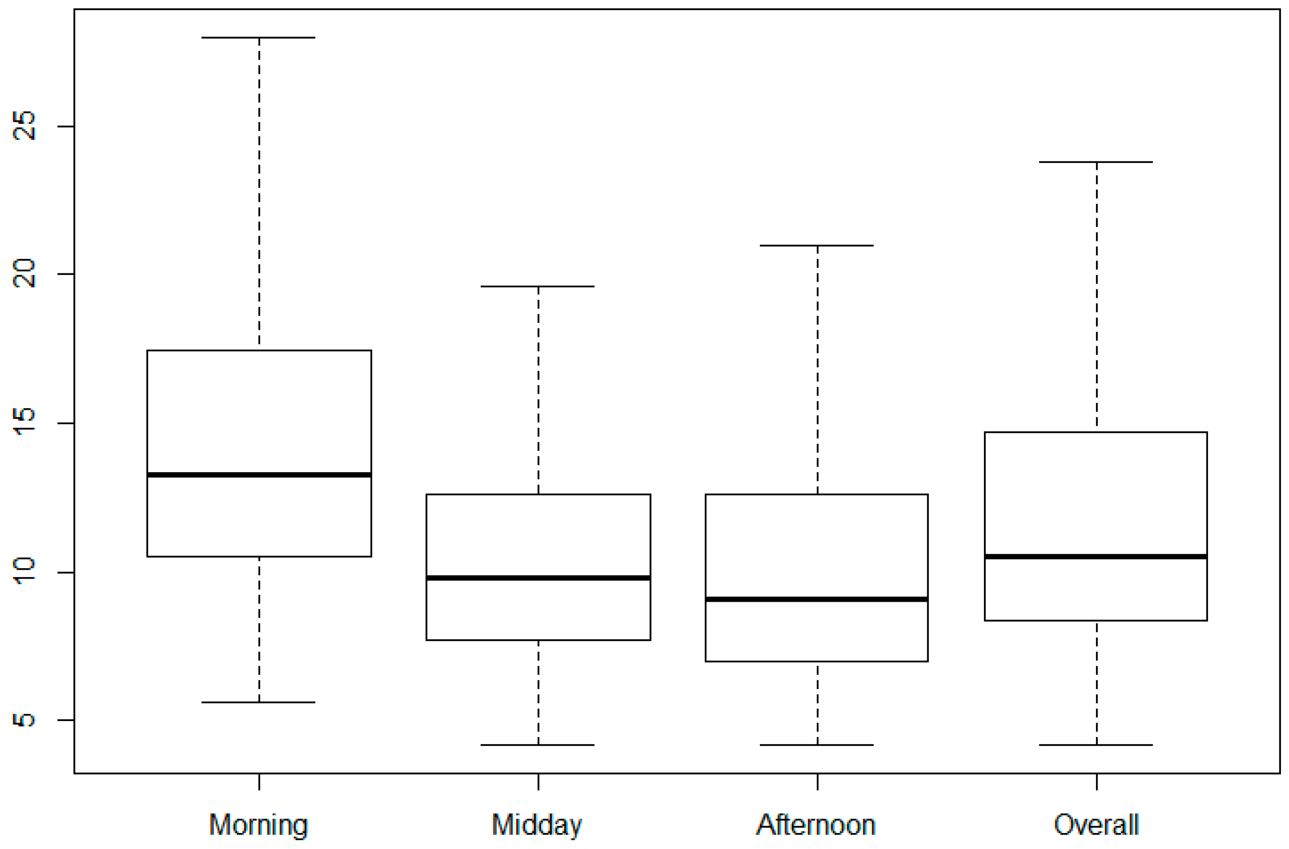
  • Does roadside exposure to pollution vary significantly with the time of day?
  • How different are roadside PM2.5 concentrations from those measured at nearby air quality monitoring stations?
  • How well can our agent-based traffic model predict traffic in the Randwick study area?
The RAPS campaign study area, Randwick, is a metropolitan area located 6 km away from the Sydney central business district. Randwick is home to extensive suburban areas, numerous recreational parks and public institutions, including schools, a large public hospital, and a major university (the University of New South Wales) located on the main road, Anzac Parade. The area has a growing population of approximately 140,000, which has increased by 20% over the last decade (ABS 2016, 2006). A New South Wales Office of Environment and Heritage (OEH) air quality monitoring station is located approximately 2 km southeast of the study site, which records meteorological variables and particulate matter (including PM2.5 and PM10). In terms of public transportation, Randwick is currently only served by buses, leading to high pedestrian activity, including waiting at bus stops and walking along footpaths.

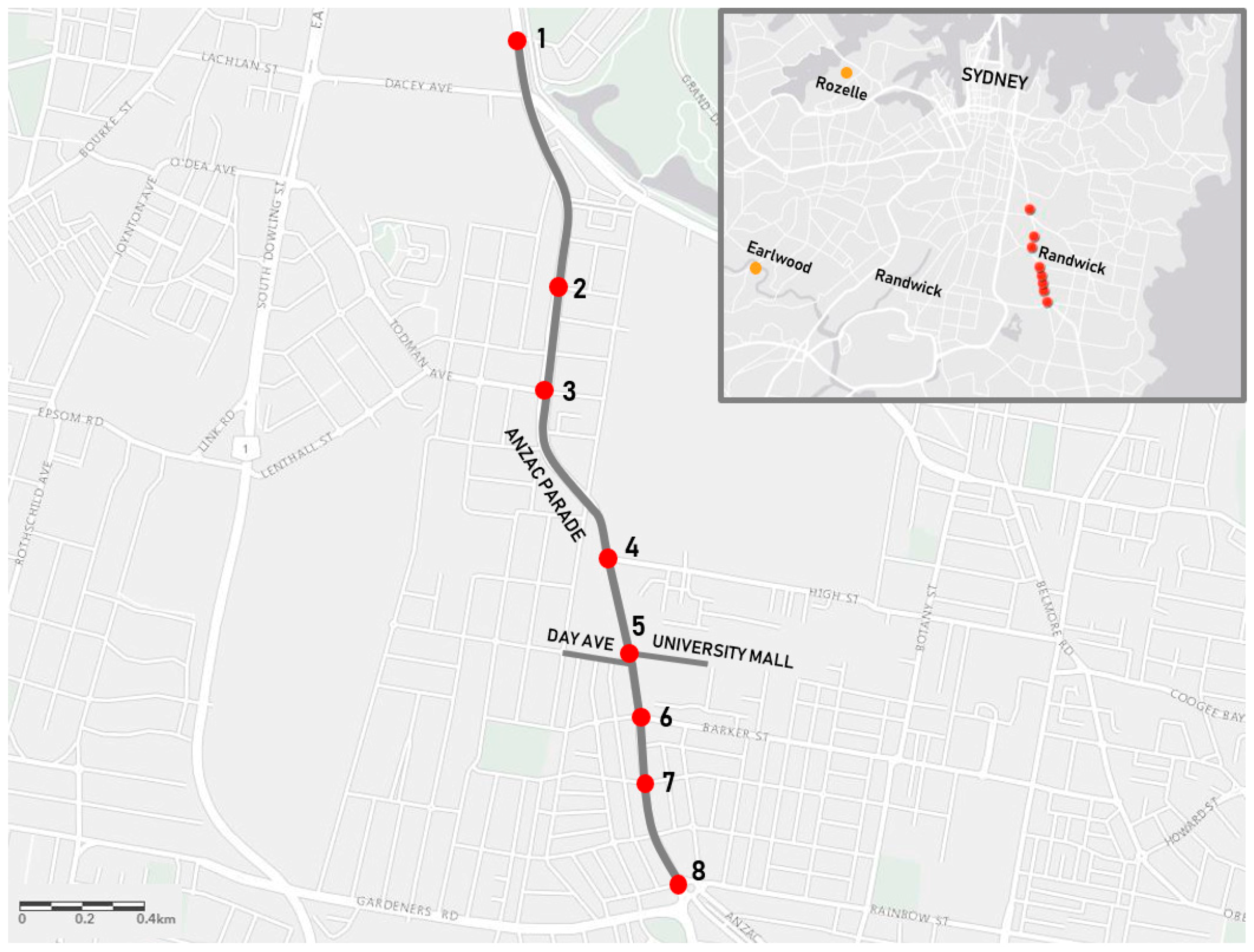
2.2. Measurement Route and Study Area

The route chosen was along a major road, Anzac Parade, which is a 4 to 6 lane main road which connects to the major M1 motorway at the northern end. The sampling route along Anzac Parade stretched for approximately 3 km, from the northern location 1 near the intersection of two busy roads, south to the roundabout at location 8 (see Figure 1). To investigate the behaviour of PM2.5 with increasing distance away from a main road, two transects were conducted perpendicular to Anzac Parade, extending 220 m (4 blocks) along Day Avenue and back to Anzac Parade, and 260 m along University Mall and back to Anzac Parade (Figure 1). Day Avenue was selected as it represented a typical Sydney residential street: Two lanes with single/double storey houses on either side. University Mall was chosen as it is a pedestrianized street (a part of the University of New South Wales campus) to provide a scenario to show how concentrations of pollution changed with distance away from the traffic.
The route was designed to include numerous bus stops and traffic intersections along the main road and to incorporate areas of varying traffic volume. For example, the main road of Anzac Parade was expected to result in a higher traffic volume than the residential Day Avenue. Data was collected from the 13th to 16th February 2017 from 0700 to 1900 h (local time), a time period which represented normal school-hour and work-week traffic conditions. The total length of the route was 7.0 km, which took an average of approximately 3 hours to cover, including waiting times for counting traffic at intersections (see next section for details).

2.3. Data Collection and Analysis

2.3.1. PM2.5 Measurements

A DustTrak DRX Aerosol Monitor (Model 8533, TSI Inc.) was used to measure PM2.5 concentrations for all mobile data collection. This utilises a 90° light-scattering laser photometer and has an aerosol concentration range of 0.001 mg/m3 to 150 mg/m3 with a resolution of ±0.1% (for a reading of 0.001 mg/m3). Air was drawn into the sensing chamber continuously using a diaphragm pump at a flow rate of 3.0 L/min. PM2.5 concentrations were measured at a time resolution of 5 seconds. The instrument’s zero calibration was set before the beginning of each section of the route using a Polyethersulfone Membrane zero filter. DustTrak DRX monitors are calibrated with Arizona Road Dust (ISO 12103-1) in-factory, which is representative of a wide range of ambient aerosols and enables calculation of the photometric calibration factor and of the size calibration factor. While DustTrak 8533 monitors have some limitations (discussed in Section 2.3), these monitors have been successfully used in previous aerosol studies and have particular benefits in mobile monitoring due to their portable nature and concentration range detected (e.g., [46,49,50,51]).
During the testing phase for the project, the DustTrak was mounted on a trolley, but this proved cumbersome to manoeuvre. During the main RAPS campaign, the DustTrak was mounted in a pram, referred to as the Mobile Air Quality Station (MAQS), to mimic the roadside particulate exposure that an infant in a pram or a child would experience (shown in Figure 2). The instrument was situated at a height of 0.78 m and a team of nine students alternated shifts in pushing the MAQS following the route shown in Figure 1. Data collection began at the intersection of Day Avenue and Anzac Parade and followed this route: Anzac Parade heading south; Day Ave heading west; Day Ave heading east; Anzac Parade heading south to location 8; Anzac Parade heading north; University Mall heading east; University Mall heading west; and then Anzac Parade heading north. This route was repeated throughout the day. A total of 71 sections were walked over the four days, resulting in approximately 68 km walked overall.
Throughout the data collection campaign, the MAQS was pushed within 1 m of the road, always on the sidewalk, and field notes were taken to record the presence of any influences that could result in an increased PM2.5 concentration (such as heavy-duty vehicles, roadworks, construction sites, and pedestrian smokers). Additionally, the time was recorded when each road intersection was reached to compare with and validate the Global Positioning System (GPS) data recorded, and the time and location was recorded at each traffic-counting site. When calculating average PM2.5 concentrations, outliers were identified using the “boxplot.stats” function in the statistical package, “R” [52], which identifies outliers as exceeding 1.5 times the inter-quartile range.
A number of studies have shown the DustTrak to be influenced by humidity and aerosol composition, which interferes with the light-scattering techniques employed, resulting in an overestimation of PM2.5 [53,54,55]. A comparative study completed at a similar time to the field campaign (July 2015–January 2017) evaluated the correlation between two DustTrak 8533-DRX units and the FEM BAM5014i at a site located in the NSW Air Quality monitoring network (Newcastle Air Quality Monitoring Station) [54]. This study reported the BAM:DustTrak PM2.5 ratio was 1.00:1.43 (for a non-heated inlet) and we have adjusted down all the raw PM2.5 data collected with the DustTrak by this factor to provide our best estimate of PM2.5 concentrations from the measurements.

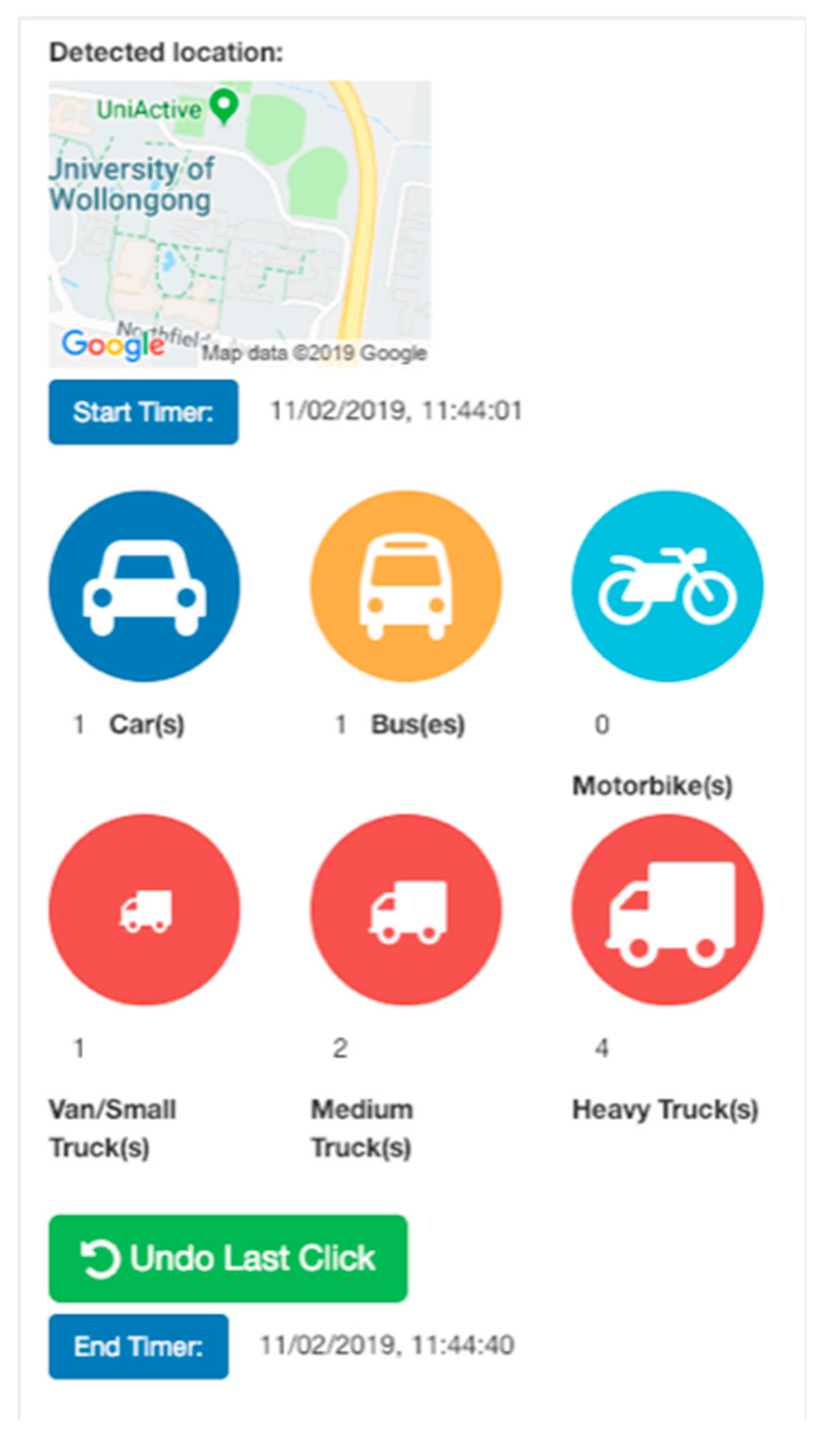
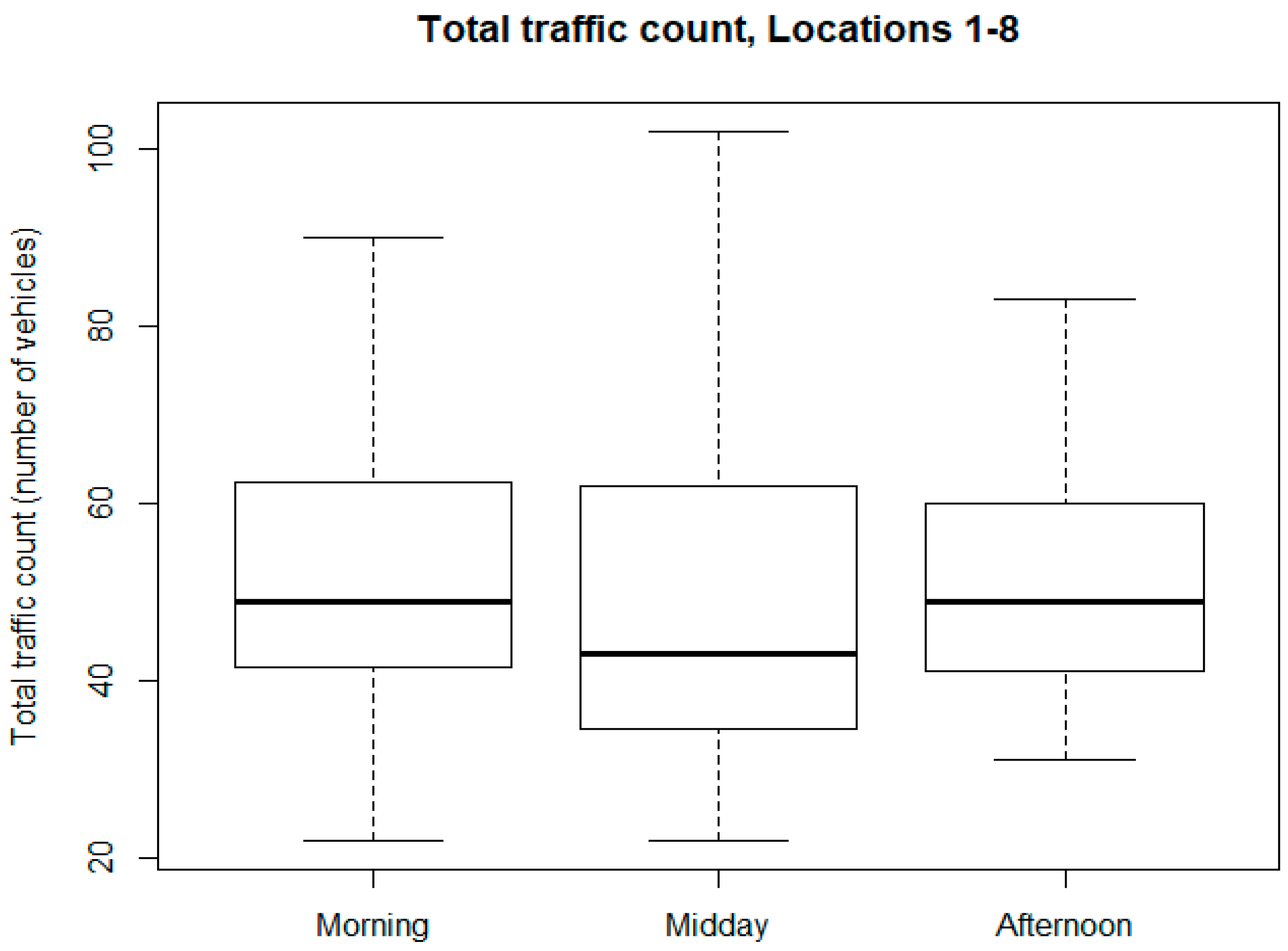
2.3.2. Traffic Counting

One of the aims of the RAPS campaign was to evaluate the performance of the agent-based modelling framework in the study area. Vehicle counts were performed by individuals visually at 8 intersections and signalised pedestrian crossings along Anzac Parade whilst completing repeated roadside transects as part of the MAQS monitoring campaign. Each time the traffic monitoring location was visited as part of these transects, traffic monitoring was conducted for three consecutive periods at each location. One traffic counting period was defined as one red to green to red traffic light cycle. Instead of cumbersome, expensive off-the-shelf devices, the traffic counters used tablets with the web-based SMART Traffic Counter app ([56], Figure 3). They counted vehicles traversing the exit lanes of each intersection (only vehicles travelling along Anzac Parade were counted). The app is browser-based, and can be used on any device with a touch-screen. In this study, it was installed on computer tablets with mobile phone network connections. It classified vehicles into 6 categories: Cars, buses, motorcycles, and 3 sizes of trucks. Counts were date-stamped to the local internet time, geo-located using the device’s GPS, and stored in a cloud-based database. Where network connection was absent or poor, data was stored locally until reception improved. The app was very well received by the field workers, since it was easy to use, had a familiar-looking interface, and gave near-instant feedback of the data stored. There was the added benefit that it removed the extra time required for transcription and eliminated the errors that are incurred by entering data from a paper-based system.

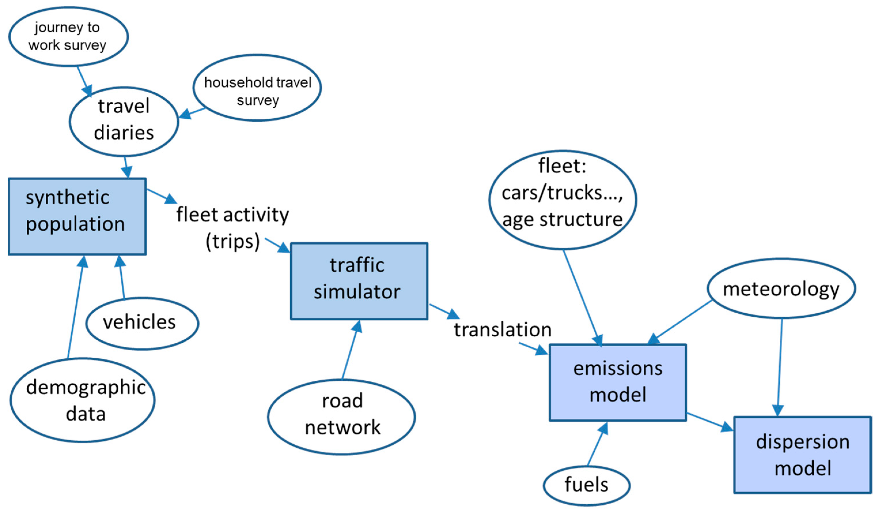
2.4. Traffic Emissions Modelling Framework

The traffic emissions model framework (Open Source Traffic Emissions Framework) comprised 4 parts (Figure 4): A synthetic population, and chained simulations for traffic, emissions, and dispersion. The synthetic population ([57]) of 110,000 residents of south-east Sydney gives a detailed model of the population of vehicle drivers in the area and their trips (such as to work, to school, or for shopping) each day. Fleet age was derived from registration data. These trips were then implemented as a route on the road network by an agent-based traffic model [58,59]. This model includes the capacity for re-routing, based on expected/perceived conditions ahead. Some drivers (‘agents’ within the model) will just take the shortest path to their destinations; others will change direction according to the state of local traffic. This approach reduces processing demands and means that the model scales well to large road networks.
The model locates each vehicle on a road segment (link) on the network for every 1-second time-step. Vehicles remain on a link for a time that depends on link properties, such as length, speed limit, capacity, and the number of other cars present. The mesoscopic level of detail does not account for lane-changes, acceleration, and braking. Traffic emission simulations are most accurate when they are informed by detailed vehicle movement data [60]. In translation software, second by second speed/time data was added, according to road size and traffic conditions, modelled in the Australian Composite Urban Emissions Drive Cycle. For every second, for every vehicle, the software calculated a parameter (“operating mode” or “opmode”) derived from vehicle type, speed, and acceleration. This data was aggregated to 60-minute intervals and input to the emissions software, MOtor Vehicle Emissions Simulator (MOVES) [61]. This software is created and maintained by the United States Environmental Protection Agency (US EPA). It is freely available and the latest version, MOVES 2014b, was released in December 2018 ([61]). Both inputs and outputs are detailed; it calculates a comprehensive suite of pollutants, including emissions from exhaust, crankcase leaks, fuel evaporation, brake wear, and tyre wear, accounting for variations related to starting, running, idling, accelerating, and braking. The Operational Street Pollution Model (OSPM) was chosen to model dispersion [62]. OSPM is a reasonably straightforward framework for simulating dispersion in street canyons.

3. Results and Discussion

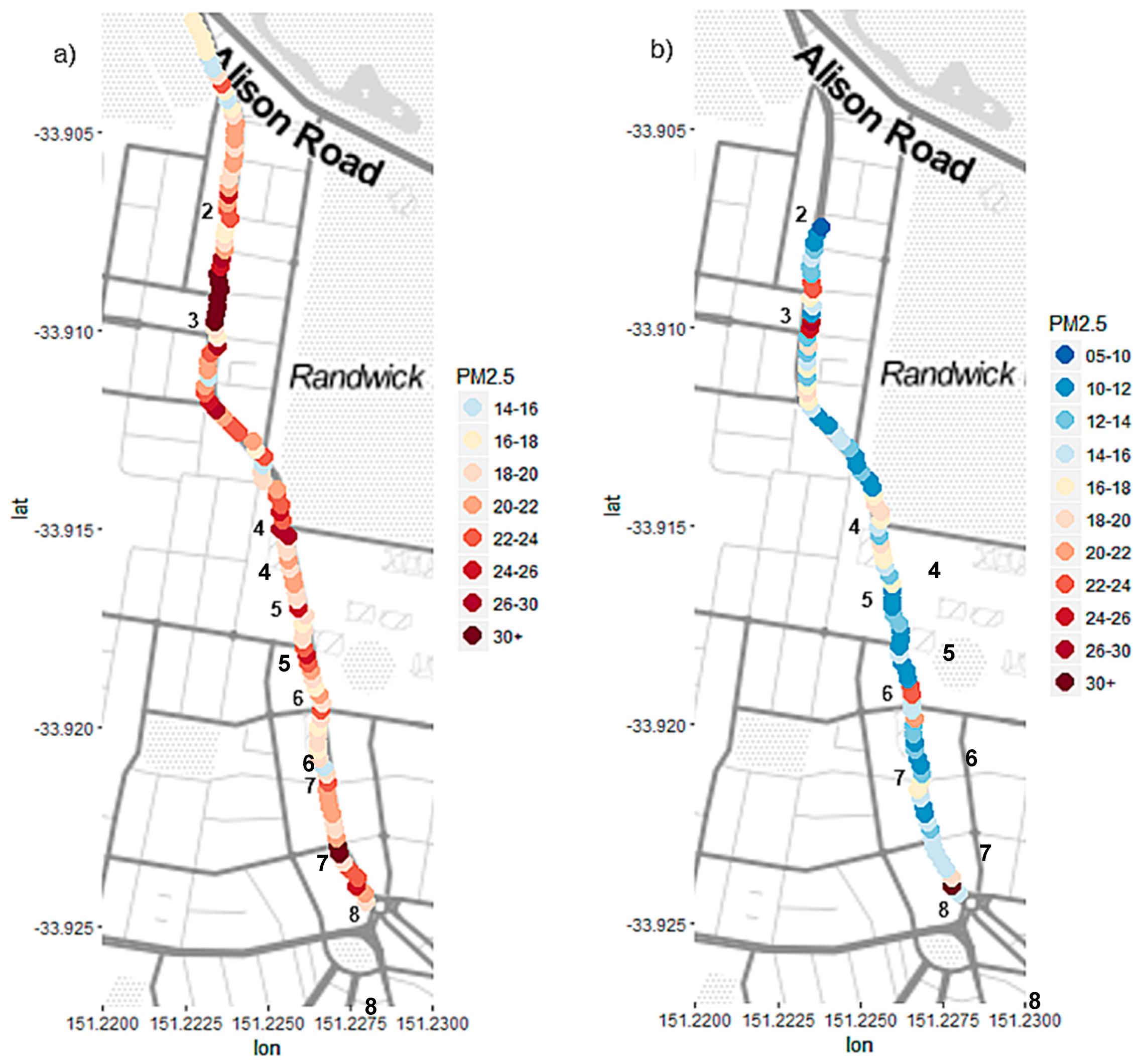
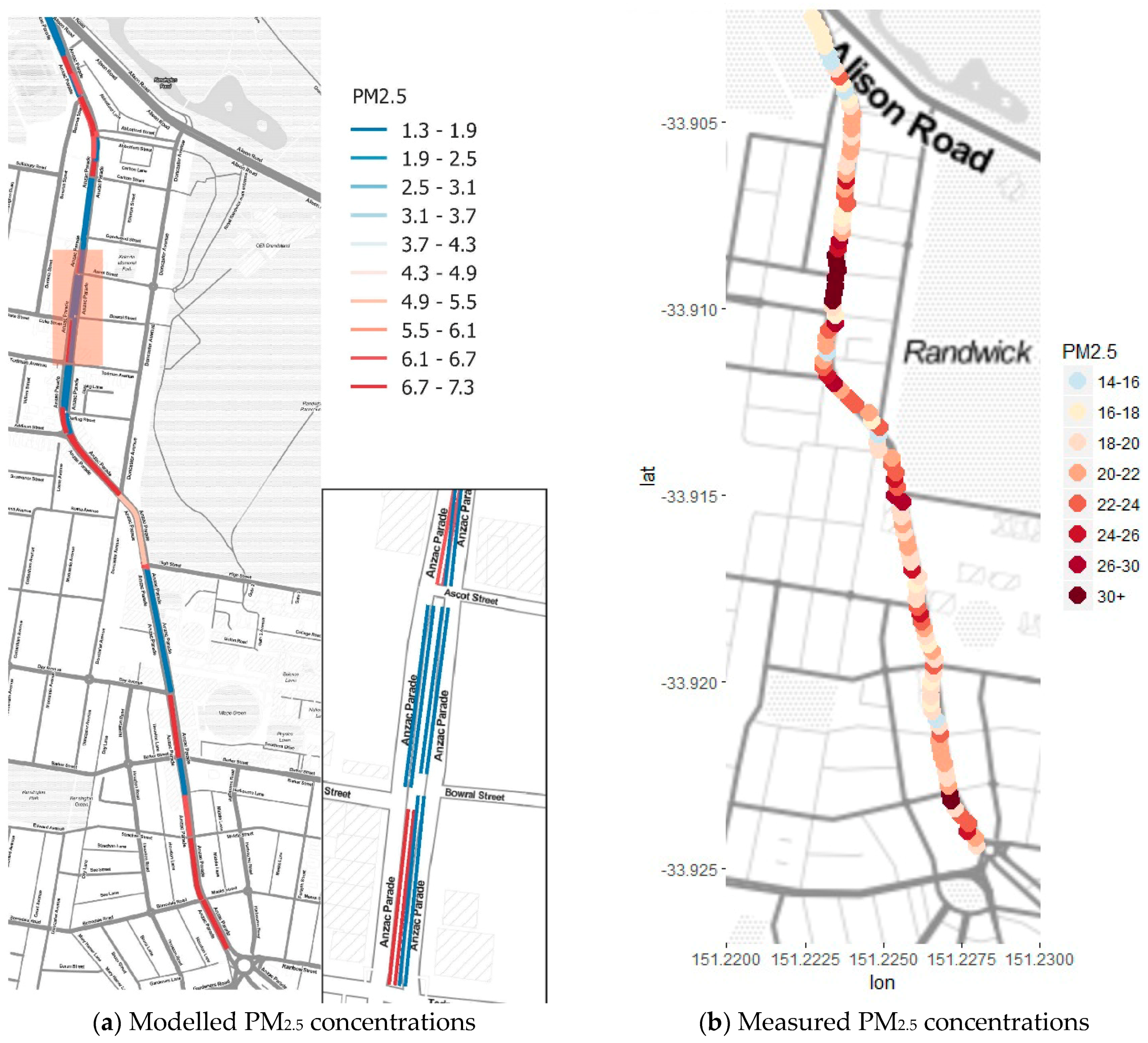
3.1. Spatial Variability and Pollution Hotspots

Significant spatial variability in PM2.5 was observed along the main road (Anzac Parade). In addition, average PM2.5 concentrations along Anzac Parade were approximately 30% higher overall than PM2.5 measured perpendicular to the main road (on Day Avenue and University Ave).
Figure 5 shows the spatial variation of PM2.5 along Anzac Parade averaged over all study days separating morning and afternoon time periods. These averages provide an indication of the spatial variability observed in the study period. Along Anzac Parade, areas of increased PM2.5 concentration (or “hotspots”) were noted at traffic intersections and areas of roadworks (shown by the dark red area between 33.908°S and 33.910°S in Figure 5a). The construction work provides an unwanted additional pollution source, since this is not typically present at urban roadside locations. The measurements made in this area (33.908°S and 33.910°S) were removed from the dataset to avoid this bias (for an indication of the magnitude of this potential bias: If the construction area data is retained, the average PM2.5 measured along the route is larger by 3%). While the average calculated PM2.5 concentration of 13 µg/m3 is within the World Health Organization (WHO) safe threshold of 25 µg/m3 (daily average mean), these “hotspot” areas along the main road largely exceed this number.
While there is evidence of increased concentrations at traffic intersections (seen most clearly in Figure 5a at the intersection of streets), the average change in PM2.5 with increasing distance from the intersection varied considerably between all intersections studied (locations 1, 2, 3, 5, 6, and 7), suggesting the influence of more local mixing factors on pollutant dispersion. Nevertheless, RAPS data as plotted in Figure 5 provides qualitative evidence of increased pollution at traffic lights and intersections that can result from stop-start and acceleration patterns at these points. It is clear from Figure 5 that roadside PM2.5 concentrations are highly spatially variable. This means that if a long-term roadside air quality monitoring station were to be established, then the average concentration of PM2.5 measured would depend strongly on where the station was located. It is not obvious that such a roadside air quality monitoring station would enable a better understanding of overall roadside PM2.5 levels that can be deduced by estimating increases in PM2.5 at the roadside over regional concentrations (as measured in nearby regional air quality monitoring stations). In Section 3.3, we attempt to estimate what the average increase of PM2.5 was at the roadside compared to the regional background during the RAPS campaign. This estimate is an indicative measure of the likely increased exposure to PM2.5 that can be expected at roadside locations compared to the concentrations measured at regulatory monitoring sites. In the longer term, the use of several fixed sensors, along a number of major roads, would provide a more detailed and accurate assessment of roadside air quality in Sydney than a full scale permanent monitoring station at a single location.

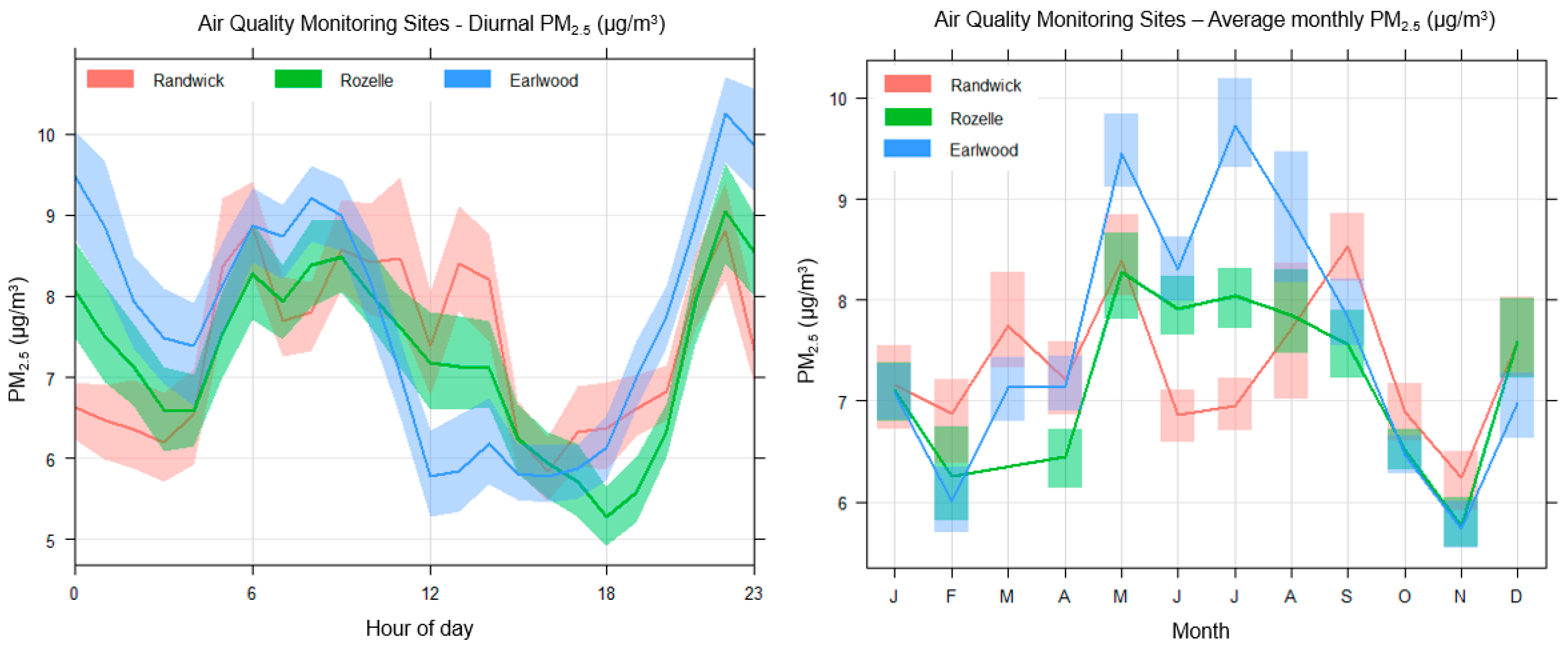
3.2. Temporal Variability in Observed PM2.5 Concentrations

The overall average roadside PM2.5 concentration measured was 13 µg/m3, with daily average PM2.5 concentrations varying only slightly between days of data collection. Daily average PM2.5 concentrations ranged from 10 to 15 µg/m3. A more noticeable variation was observed between runs collected on the same day, depending on the time of day and location.
Periods of heightened vehicle activity were identified—the morning ‘rush hour’ was defined from 7:00 to 9:30, a midday period was defined from 9:30 to 16:00, and an afternoon rush period was defined from 16:00 to 19:00. Overall, PM2.5 averages appear to be significantly higher in the morning rush hour (with a mean and standard deviation of 15 ± 3 µg/m3) compared to the midday and afternoon periods (both with a mean of 11 µg/m3 and standard deviations of ±2 to 3 µg/m3) (Figure 6). Morning, midday, and afternoon PM2.5 levels were shown to be normally distributed. Morning PM2.5 concentration was shown to be statistically significantly different to midday and afternoon PM2.5 concentrations using Welch’s unequal variances t-test (p-values = <0.0005). Midday PM2.5 was shown to not be statistically significantly different from afternoon PM2.5 levels (p-value = 0.494).
Average traffic volume (based on traffic counts) varied within 10% of the mean vehicle count recorded at morning, midday, and afternoon hours, hence increased PM2.5 of this magnitude is unlikely due to increased traffic volume (Appendix B). These findings are in agreement with existing roadside studies, which have identified similar patterns due to influences from traffic emissions [29]. Additional effects leading to this heightened PM2.5 concentration in the morning may include a lower boundary layer height associated with the diurnal temperature cycle and a reduction in associated wind-speed, which limits atmospheric mixing [63,64]. Over the study period, the average wind speed and air temperature measured at the Randwick Air Quality Monitoring site was approximately 30% and 12% lower in the morning compared to the afternoon, respectively (Appendix C). The significantly worse PM2.5 pollution experienced in the morning rush-hour implies that this is a bad time for individuals to choose to engage in high intensity exercise, such as jogging or cycling, near main roads.

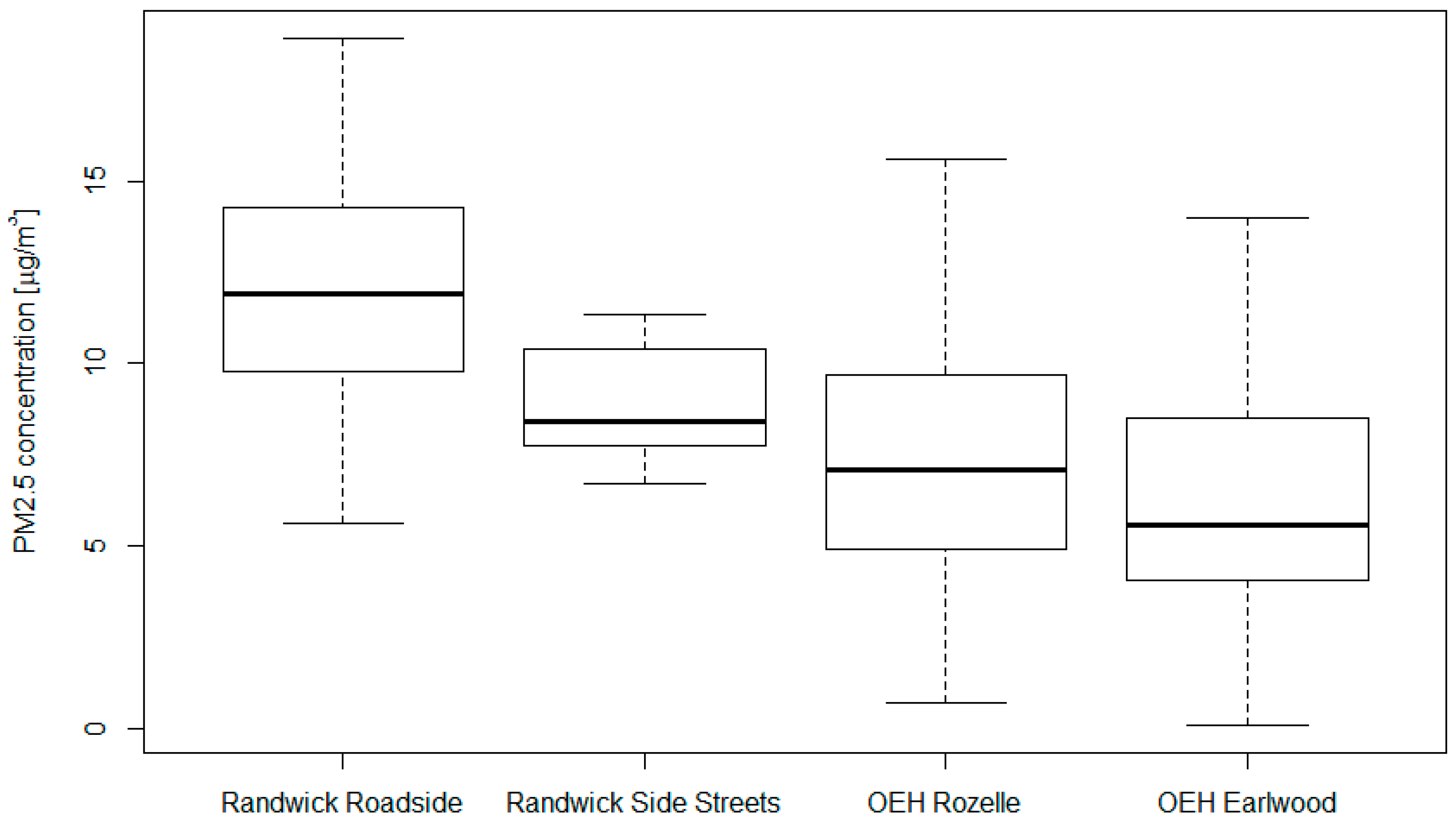
3.3. Comparison with Air Quality Monitoring Station Data

The primary aim of the RAPS study was to try to answer the question posed at the Clean Air and Urban Landscapes public forums, by providing an estimate of how much worse PM2.5 pollution was at the roadside than at the nearby ambient air quality monitoring stations. This task was complicated by the fact that during the RAPS campaign period, PM2.5 data at the closest OEH monitoring station (Randwick at 33° 56’ 00”S, 151° 14’ 31” E) was not available. For this reason, PM2.5 data from the next closest monitoring stations were used instead, Earlwood at 33° 55’ 04” S, 151° 08’ 05” E (about 10 km to the west of Randwick) and Rozelle at 33° 51’ 57”S, 151° 09’ 45” E (about 8 km to the northeast of Randwick).
We therefore firstly set out to determine how comparable PM2.5 concentrations were at the three sites, Randwick, Earlwood, and Rozelle, when all stations were measuring PM2.5. Data were extracted from the OEH database from 1/4/2017 to 30/11/2018 (20 months) from all three sites for daytime hours only (07:00–19:00) to align with measurement times in the RAPS campaign.
Figure 7 shows the diurnal and monthly patterns of PM2.5 measured at each site. The diurnal pattern recorded at each of the three sites is similar, observing an increase in PM2.5 throughout the morning, decreasing to the afternoon, and a peak again approaching midnight. The monthly averages show that some variation exists between the three sites, although this variation is lowest during summertime months. Overall, the three stations predominantly show similar variations in PM2.5 concentrations. This provides qualitative evidence that the data from these sites is broadly comparable and the three air quality stations are measuring similar regional ambient PM2.5 concentrations. In other words, Randwick is not significantly more (or less) polluted than the other sites in the summertime.
In order to provide more quantitative evidence, a statistical analysis was conducted to compare the 20 months of data from Randwick, to the data from the Rozelle and Earlwood air quality monitoring stations. We found that the PM2.5 observations from the three sites were generally comparable, with both stations reporting an index of agreement of 0.99 compared to Randwick (perfect agreement would have an index of agreement of 1.0) [65]. The mean bias between Randwick and Rozelle was 0.17 µg/m3 (equivalent to a normalized mean bias of 2.2%) and between Randwick and Earlwood was 0.51 µg/m3 (equivalent to a normalized mean bias of 6.9%). From this we concluded that use of the Rozelle and Earlwood PM2.5 data in place of the missing PM2.5 data from the ambient air quality monitoring station at Randwick is justified, within an uncertainty of ±10%.
The next step was to compare the roadside measurements made during the RAPS campaign to the coincident measurements made at Rozelle and Earlwood. Table 2 shows the average PM2.5 concentration (along with the 1σ standard deviation) recorded at each monitoring station and at the roadside in Randwick during the RAPS campaign. In this analysis, only the PM2.5 data measured on the main roads was used. Concentrations are given for the whole campaign and separately for the morning, noon, and afternoon times described in Section 3.2 so that temporal patterns may be seen. The side-street data is shown in comparison to the main road and ambient air quality monitoring stations in Figure 8 to illustrate the broad-scale spatial variability.
Overall, during the RAPS campaign, roadside PM2.5 concentrations were approximately double those measured at Rozelle and Earlwood, with roadside values on main roads increased by an estimated 6 µg/m3 over regional ambient values. During the morning rush-hour period, roadside PM2.5 concentrations were more than twice the background amounts as measured at Earlwood and Rozelle (with an increase of 8 µg/m3 over ambient background PM2.5 values). Statistical testing using the Mann-Whitney test (for non-normally distributed data) showed that roadside PM2.5 levels were found to be statistically significantly different in comparison to Rozelle and Earlwood monitoring stations over morning, midday, and afternoon periods (all p-values < 0.005). It should be noted that there are larger differences between observations at Rozelle and Earlwood for this short time period than were found for variations between months in the 20-month record described above (Figure 7). This temporal variation will contribute further uncertainty to our findings regarding the magnitude of roadside increases in PM2.5.
The PM2.5 observations from the ambient air quality monitoring stations at Earlwood and Rozelle did not exhibit the substantially higher PM2.5 concentrations during the morning rush-hour time (07:00–09:30) compared to the midday (09:30–16:00) and afternoon rush (16:00–19:00) times. This provides further evidence that the morning rush increases in the Randwick roadside measurements are likely due to the local traffic emissions being emitted into a stable atmosphere with low mixing and reduced dispersion due to a low planetary boundary layer height at this time of day [63,64]. Increases in PM2.5 concentrations such as these are therefore likely to be replicated alongside other major roads of similar traffic volume within the greater Sydney region. While the exact level of PM2.5 increases will vary between sites and on different days, this study provides an indicative estimate of the likely magnitude of that increase on main roads of 6 µg/m3 and for side-streets of 3 µg/m3. In addition, increases are expected to be significantly worse in the morning peak traffic times (8 µg/m3) compared to other times during the day (averaging approximately 4 µg/m3). Given that the Australian legislative target for PM2.5 concentrations is 8 µg/m3 or less, averaged over the year [66], these increases represent a significant additional air quality risk to those who spend significant amounts of time roadside in their typical day.
The RAPS campaign was motivated by public interest in the possible discrepancy between PM2.5 concentrations measured at ambient air quality monitoring stations and those experienced by citizens as they go about their daily business in the vicinity of busy roads. The increases of PM2.5 over ambient background levels measured during the RAPS campaign can only be considered indicative of the likely increases that may be experienced at busy roadside locations in Sydney, since the RAPS campaign gathered data for a single area over four days at one time of the year. Nevertheless, the increases over ambient background PM2.5 concentrations observed during RAPS were substantial and significant, such that we infer the following generalisations:
  • Roadside PM2.5 concentrations by main roads are likely to be significantly higher than indicated by the nearby ambient air quality monitoring stations.
  • Actual concentrations of PM2.5 are highly variable with hotspots near major intersections and places where vehicles accelerate (e.g., bus-stops).
  • This means that locating a single air quality monitoring station at a roadside location will only show the pollution levels at that one specific location: Measurements at a large number of locations are needed to estimate pollution exposure for pedestrians as they walk along main roads.
  • The increases in PM2.5 concentrations estimated here of 6 µg/m3 overall and 8 µg/m3 during the morning rush hour provide our first indicative estimate of likely additional exposure to PM2.5 (over the ambient air quality) for pedestrians walking along main roads in Sydney.
  • We recommend walking along side-streets where possible, since the traffic related increase in PM2.5 of 3 µg/m3 that we observed on the side-streets was approximately half that observed along the main streets.
  • Extra thought should be given to locating al fresco dining outlets along main roads given the likely additional exposure for those working roadside all day long.

3.4. Testing the Traffic Model

Our traffic model’s performance was disappointing, with predicted traffic volume poorly correlated to actual traffic counts and an overall four-fold underestimation of traffic volume by the model. The model did predict significant variation in the PM2.5 emissions along the main road in a similar fashion to the highly variable concentrations observed, with hotspots predicted in certain links and at intersections. This is illustrated in Figure 9 with the modelled PM2.5 emissions in g.hr−1 shown on the left hand-side and an example of one day’s measured PM2.5 concentrations in µg/m3 shown on the right-hand side. The modelled emissions show very substantial spatial variation with hotspots at junctions and traffic lights and lower values along free-flowing sections of the road, much like the observations. As well as some inaccuracies in the predicted traffic volumes there is also a large discrepancy around the site of construction work, which highlights this additional temporary source of additional PM2.5 pollution in the area that is not associated with traffic.
The four-fold under-prediction of traffic volume by the model had two major causes: The model did not account for vehicles that came from outside the study area and heavy vehicles were not modelled. Heavy duty (diesel) vehicles comprise approximately 22% of PM2.5 emissions from total vehicles in the NSW Greater Metropolitan Region, whereas light-duty vehicles (diesel and petrol) account for 18% of PM2.5 emissions [67]. Hence, a significant factor in PM2.5 emissions is missing from the model by not including heavy vehicles.
Through traffic and vehicles from outside the area were likely to have been a significant fraction of the traffic on Anzac Parade. A number of sites in the area may account for traffic volume, including Sydney airport to the south, the University of New South Wales set on this arterial road, and a major hospital next to the university. The road is also heavily used by public buses.
This first testing of an agent-based traffic model within one suburb of Sydney has shown that modelling of a much larger area will be needed for accurate modelling of traffic volumes. Due to the very large computing resources required to scale up to a much greater area, this was not possible within this study. Nevertheless, the model’s ability to correctly capture the large spatial variability of PM2.5 emissions (which are replicated in the resulting observed concentrations) indicate that this approach shows some promise for future studies using a much larger area in the model.

4. Summary and Conclusions

Motivated by questions posed at public forums run by the Clean Air and Urban Landscapes hub, we aimed to estimate to what extent the air quality deviated from that reported by the legislative monitoring network in NSW at two case study sites. The first case study was the Auburn-WASPSS campaign, which aimed to represent a typical second-story suburban balcony (reported in a companion paper [44]), whilst the second was a busy roadside location (the RAPS campaign reported here).
During the RAPS campaign, roadside PM2.5 concentrations were measured to indicate the personal exposure of a vulnerable demographic (in-pram babies). Mean roadside PM2.5 concentrations were 13 µg/m3 (approximately double those at the nearby regulatory air quality network sites), representing an increase of ~6 µg/m3 above regional background values. Our analysis showed that roadside PM2.5 concentrations during the morning rush hour are approximately 50% higher than during other parts of the day, and increases on side-streets were approximately half those measured on the main roads.
Hotspots along the main road corresponded to areas of increased traffic congestion, resulting in a higher PM2.5 exposure. The RAPS campaign provided evidence that the PM2.5 exposure at a roadside level is not accurately represented by air quality monitoring stations, which largely underrepresent PM2.5 concentrations and do not reflect increased exposure in a roadside environment with close proximity to traffic.
The agent-based traffic model significantly under-estimated the numbers of vehicles and emissions estimates by about 4 times (in comparison to measurement amounts). This was most likely due to omission of through traffic and heavy vehicles. The modelling framework showed promise, but the study demonstrated the need to generate more comprehensive input data for the traffic model over a much wider region.
Our findings suggest that those working for long hours at busy roadside locations are at greater risk of suffering detrimental health effects associated with higher levels of exposure to PM2.5. Furthermore, the worse air quality in the morning rush hour means that, where possible, joggers and pedestrian/cyclist commuters should avoid busy roads around these times to reduce repeatedly increased PM2.5 exposure. Further studies quantifying the health impacts of these roadside PM2.5 increases are recommended to evaluate the impact on susceptible populations, including infants and the elderly.
We conclude from the WASPSS-Auburn campaign that the existing air quality monitoring network in New South Wales provided a good representation of the air quality at the Auburn balcony site selected for this study. Although this result cannot be generalised to all balconies, it demonstrates the effectiveness of a regional air quality monitoring network in western Sydney. In contrast, roadside PM2.5 concentrations observed in the RAPS campaign were significantly increased over those measured at nearby air quality monitoring stations. Nevertheless, the very high spatial variability measured at roadside locations implies that roadside air quality could not simply be evaluated by locating an air quality monitoring station at a single roadside location. Estimates of average increased roadside pollution levels above the regional background are needed (such as the 6 µg/m3 estimated in this study). Improved estimates could be made in the future by a network of fixed roadside sensors that operate year-round. We conclude that the existing air quality monitoring network in New South Wales is fit for purpose, but could be supplemented by public outreach programmes that alerted people to the increased pollution levels that are commonly present at high traffic areas and simple steps that can be taken to minimise exposure.

Author Contributions

I.W. formal analysis, methodology, validation, investigation, writing—original draft, writing—review and editing, visualization. C.P.-W. conceptualization, methodology, investigation, resources, writing—original draft, writing—review and editing, supervision, funding acquisition, project administration. H.F. software, validation, formal analysis, investigation, writing—review and editing, visualization. M.A.: software. P.P.: investigation, resources, É.-A.G. data curation, software, writing—review & editing. O.G. investigation. P.K. formal analysis, supervision, writing—review & editing.

Funding

This research was funded by the Clean Air and Urban Landscapes hub, which is supported by the National Environmental Science Program and by the University Global Partnership Network for funding via the NEST-SEAS (Next-Generation Environmental Sensing for Local To Global Scale Health Impact Assessment) project.

Acknowledgments

Thanks to the team of students and interns who took part in the RAPS campaign (Alexander Kuhar, Lachlan Spicer, Jenny Xu, Kate Sneesby, Stephanie Beaupark, Hamish McDougall, Lewis McCloud, Monica Sharma and Sally Smith). Thanks also to John Kirkwood of NSW OEH for loan of the DustTraks instrument deployed.

Conflicts of Interest

The authors declare no conflict of interest.

Appendix A

Table A1. Traffic counting locations and description.
Location NumberLocationDescription
1Pedestrian crossing North of Anzac Pde and Allison St.Pedestrian crossing over a 6-lane road, golf course and parkland surrounding.
2Anzac Pde and Goodwood St.Traffic intersection of a 6-lane road and a 2-lane road, building height 1-5 stories.
3Anzac Pde and Todman Ave.Traffic intersection of a 5-lane road and a 6-lane road, building height 2 stories.
4Anzac Pde and High St.Traffic intersection of a 6-lane road and a 4-lane road, building height 1-2 stories.
5Anzac Pde and University Mall.Traffic stop intersecting 6-lane road and large pedestrian walkway. At time of study period, only 4 traffic lanes operational.
6Anzac Pde and Barker St.Traffic intersection of two 4-lane roads, building height ranges from 1-8 stories.
7Anzac Pde and Strachan St.Traffic intersection of two 4-lane roads, building height approximately 2 stories.
8Pedestrian crossing above the 9-ways roundabout. Pedestrian crossing over 4-lane road, building height approximately 2 stories.

Appendix B

Figure A1. Total traffic count calculated as the sum of cars, buses, trucks, and bikes. Data includes all eight traffic monitoring stations, and is separated into morning (07:00–09:30), midday (09:30–16:00), and afternoon (16:00–19:00). The black lines are the median values, and the box includes the upper and lower quartiles (inter-quartile range). The whiskers extend to 1.5× the inter-quartile range. For clarity, outliers were removed from the figure if they exceeded beyond the edge of the whiskers.
Atmosphere 10 00217 g0a1

Appendix C

Figure A2. (left) Hourly wind speed (m/s) and (right) hourly air temperature (°C) measured at the Randwick Air Quality Monitoring site (33° 56’ 00”S, 151° 14’ 31”E). Data subsetted into morning (07:00–10:00), midday (10:00–16:00), and afternoon (16:00–19:00) sections to align with temporal study subsets. The black lines are the median values, and the box includes the upper and lower quartiles (inter-quartile range). The whiskers extend to 1.5× the inter-quartile range. For clarity, outliers were removed from the figure if they exceeded beyond the edge of the whiskers. Data retrieved from NSW OEH, https://www.environment.nsw.gov.au/AQMS/search.htm.
Atmosphere 10 00217 g0a2

References

  1. Cohen, A.J.; Brauer, M.; Burnett, R.; Anderson, H.R.; Frostad, J.; Estep, K.; Balakrishnan, K.; Brunekreef, B.; Dandona, L.; Dandona, R.; et al. Estimates and 25-year trends of the global burden of disease attributable to ambient air pollution: An analysis of data from the Global Burden of Diseases Study 2015. Lancet 2017, 389, 1907–1918. [Google Scholar] [CrossRef]
  2. Segalin, B.; Kumar, P.; Micadei, K.; Fornaro, A.; Gonçalves, F.L.T. Size–segregated particulate matter inside residences of elderly in the Metropolitan Area of São Paulo, Brazil. Atmos. Environ. 2017, 148, 139–151. [Google Scholar] [CrossRef] [Green Version]
  3. Saadeh, R.; Klaunig, J. Child’s Development and Respiratory System Toxicity. J. Environ. Anal. Toxicol. 2014, 4. [Google Scholar] [CrossRef]
  4. Sharma, A.; Kumar, P. A review of factors surrounding the air pollution exposure to in-pram babies and mitigation strategies. Environ. Int. 2018, 120, 262–278. [Google Scholar] [CrossRef]
  5. Goldizen, F.C.; Sly, P.D.; Knibbs, L.D. Respiratory Effects of Air Pollution on Children. Pediatr. Pulmonol. 2016, 51, 94–108. [Google Scholar] [CrossRef] [PubMed]
  6. Clark, N.A.; Demers, P.A.; Karr, C.J.; Koehoorn, M.; Lencar, C.; Tamburic, L.; Brauer, M. Effect of Early Life Exposure to Air Pollution on Development of Childhood Asthma. Environ. Health Persp. 2010, 118, 284–290. [Google Scholar] [CrossRef]
  7. Gehring, U.; Wijga, A.H.; Brauer, M.; Fischer, P.; De Jongste, J.C.; Kerkhof, M.; Oldenwening, M.; Smit, H.A.; Brunekreef, B. Traffic-related air pollution and the development of asthma and allergies during the first 8 years of life. Am. J. Respir. Crit. Care Med. 2010, 181, 596–603. [Google Scholar] [CrossRef]
  8. Woodruff, T.J.; Parker, J.D.; Schoendorf, K.C. Fine particulate matter (PM2.5) air pollution and selected causes of postneonatal infant mortality in California. Environ. Health Persp. 2006, 114. [Google Scholar] [CrossRef]
  9. Basagaña, X.; Esnaola, M.; Rivas, I.; Amato, F.; Alvarez-Pedrerol, M.; Forns, J.; López-Vicente, M.; Pujol, J.; Nieuwenhuijsen, M.; Querol, X.; et al. Neurodevelopmental deceleration by urban fine particles from different emission sources: A longitudinal observational study. Environ. Health Persp. 2016, 124, 1630–1636. [Google Scholar] [CrossRef]
  10. Sunyer, J.; Esnaola, M.; Alvarez-Pedrerol, M.; Forns, J.; Rivas, I.; López-Vicente, M.; Suades-González, E.; Foraster, M.; Garcia-Esteban, R.; Basagaña, X.; et al. Association between Traffic-Related Air Pollution in Schools and Cognitive Development in Primary School Children: A Prospective Cohort Study. PLoS Med. 2015, 12, e1001792. [Google Scholar] [CrossRef]
  11. Gehring, U.; Gruzieva, O.; Agius, R.M.; Beelen, R.; Custovic, A.; Cyrys, J.; Eeftens, M.; Flexeder, C.; Fuertes, E.; Heinrich, J.; et al. Air pollution exposure and lung function in children: The ESCAPE project. Environ. Health Persp. 2013, 121, 11–12. [Google Scholar] [CrossRef]
  12. Heal, M.R.; Kumar, P.; Harrison, R.M. Particles, air quality, policy and health. Chem. Soc. Rev. 2012, 41, 6606–6630. [Google Scholar] [CrossRef] [PubMed]
  13. Zwozdziak, A.; Sówka, I.; Willak-Janc, E.; Zwozdziak, J.; Kwiecińska, K.; Balińska-Miśkiewicz, W. Influence of PM1 and PM2.5 on lung function parameters in healthy schoolchildren—A panel study. Environ. Sci. Pollut. Res. 2016, 23, 23892–23901. [Google Scholar] [CrossRef] [PubMed]
  14. Chan, Y.C.; McTainsh, G.; Leys, J.; McGowan, H.; Tews, K. Influence of the 23 October 2002 dust storm on the air quality of four Australian cities. Water Air Soil Pollut. 2005, 164, 329–348. [Google Scholar] [CrossRef]
  15. Rea, G.; Paton-Walsh, C.; Turquety, S.; Cope, M.; Griffith, D. Impact of the New South Wales fires during October 2013 on regional air quality in eastern Australia. Atmos. Environ. 2016, 131, 150–163. [Google Scholar] [CrossRef] [Green Version]
  16. Crawford, J.; Chambers, S.; Cohen, D.D.; Williams, A.; Griffiths, A.; Stelcer, E.; Dyer, L. Impact of meteorology on fine aerosols at Lucas Heights, Australia. Atmos. Environ. 2016, 145, 135–146. [Google Scholar] [CrossRef]
  17. Brines, M.; Dall’Osto, M.; Beddows, D.C.S.; Harrison, R.M.; Gómez-Moreno, F.; Núñez, L.; Artíñano, B.; Costabile, F.; Gobbi, G.P.; Salimi, F.; et al. Traffic and nucleation events as main sources of ultrafine particles in high-insolation developed world cities. Atmos. Chem. Phys. 2015, 15, 5929–5945. [Google Scholar] [CrossRef] [Green Version]
  18. Kumar, P.; Morawska, L.; Birmili, W.; Paasonen, P.; Hu, M.; Kulmala, M.; Harrison, R.M.; Norford, L.; Britter, R. Ultrafine particles in cities. Environ. Int. 2014, 66, 1–10. [Google Scholar] [CrossRef] [PubMed] [Green Version]
  19. Albriet, B.; Sartelet, K.N.; Lacour, S.; Carissimo, B.; Seigneur, C. Modelling aerosol number distributions from a vehicle exhaust with an aerosol CFD model. Atmos. Environ. 2010, 44, 1126–1137. [Google Scholar] [CrossRef]
  20. Kumar, P.; Morawska, L.; Martani, C.; Biskos, G.; Neophytou, M.; Di Sabatino, S.; Bell, M.; Norford, L.; Britter, R. The rise of low-cost sensing for managing air pollution in cities. Environ. Int. 2015, 75, 199–205. [Google Scholar] [CrossRef] [PubMed] [Green Version]
  21. Steinle, S.; Reis, S.; Sabel, C.E. Quantifying human exposure to air pollution-Moving from static monitoring to spatio-temporally resolved personal exposure assessment. Sci. Total Environ. 2013, 443, 184–193. [Google Scholar] [CrossRef] [PubMed]
  22. Greaves, S.; Issarayangyun, T.; Liu, Q. Exploring variability in pedestrian exposure to fine particulates (PM2.5) along a busy road. Atmos. Environ. 2008, 42, 1665–1676. [Google Scholar] [CrossRef]
  23. Kumar, P.; Patton, A.P.; Durant, J.L.; Frey, H.C. A review of factors impacting exposure to PM2.5, ultrafine particles and black carbon in Asian transport microenvironments. Atmos. Environ. 2018, 187, 301–316. [Google Scholar] [CrossRef]
  24. Bereitschaft, B. Pedestrian exposure to near-roadway PM2.5 in mixed-use urban corridors: A case study of Omaha, Nebraska. Sustain. Cities Soc. 2015, 15, 64–74. [Google Scholar] [CrossRef]
  25. Targino, A.C.; Gibson, M.D.; Krecl, P.; Rodrigues, M.V.C.; dos Santos, M.M.; de Paula Corrêa, M. Hotspots of black carbon and PM2.5 in an urban area and relationships to traffic characteristics. Environ. Pollut. 2016, 218, 475–486. [Google Scholar] [CrossRef]
  26. Goel, A.; Kumar, P. Characterisation of nanoparticle emissions and exposure at traffic intersections through fast-response mobile and sequential measurements. Atmos. Environ. 2015, 107, 374–390. [Google Scholar] [CrossRef]
  27. Schneider, I.L.; Teixeira, E.C.; Silva Oliveira, L.F.; Wiegand, F. Atmospheric particle number concentration and size distribution in a traffic–impacted area. Atmos. Pollut. Res. 2015, 6, 877–885. [Google Scholar] [CrossRef]
  28. Choudhary, A.; Gokhale, S. Urban real-world driving traffic emissions during interruption and congestion. Trans. Res. Part Trans. Environ. 2016, 43, 59–70. [Google Scholar] [CrossRef]
  29. Kumar, P.; Rivas, I.; Sachdeva, L. Exposure of in-pram babies to airborne particles during morning drop-in and afternoon pick-up of school children. Environ. Pollut. 2017, 224, 407–420. [Google Scholar] [CrossRef] [PubMed] [Green Version]
  30. Hitchins, J.; Morawska, L.; Wolff, R.; Gilbert, D. Concentrations of submicrometre particles from vehicle emissions near a major road. Atmos. Environ. 2000, 34, 51–59. [Google Scholar] [CrossRef] [Green Version]
  31. Kinney, P.L.; Gichuru, M.G.; Volavka-Close, N.; Ngo, N.; Ndiba, P.K.; Law, A.; Gachanja, A.; Gaita, S.M.; Chillrud, S.N.; Sclar, E. Traffic impacts on PM2.5air quality in Nairobi, Kenya. Environ. Sci. Policy 2011, 14, 369–378. [Google Scholar] [CrossRef]
  32. Wang, J.S.; Chan, T.L.; Ning, Z.; Leung, C.W.; Cheung, C.S.; Hung, W.T. Roadside measurement and prediction of CO and PM2.5 dispersion from on-road vehicles in Hong Kong. Trans. Res. Part Trans. Environ. 2006, 11, 242–249. [Google Scholar] [CrossRef]
  33. Goel, A.; Kumar, P. Vertical and horizontal variability in airborne nanoparticles and their exposure around signalised traffic intersections. Environ. Pollut. 2016, 214. [Google Scholar] [CrossRef]
  34. Buzzard, N.A.; Clark, N.N.; Guffey, S.E. Investigation into pedestrian exposure to near-vehicle exhaust emissions. Environ. Health Glob. Access Sci. Sour. 2009, 8. [Google Scholar] [CrossRef]
  35. Garcia-Algar, O.; Canchucaja, L.; d’Orazzio, V.; Manich, A.; Joya, X.; Vall, O. Different exposure of infants and adults to ultrafine particles in the urban area of Barcelona. Environ. Monit. Assess. 2015, 187, 4196. [Google Scholar] [CrossRef]
  36. Galea, K.S.; Maccalman, L.; Amend-straif, M.; Gorman-Ng, M.; Cherrie, J.W. Are children in buggies exposed to higher PM2.5 concentrations than adults? J. Environ. Health Res. 2014, 14, 28–42. [Google Scholar]
  37. Cooper, J.; Corcoran, J. Census of Population and Housing: Commuting to Work—More Stories from the Census, 2016. Journey to Work in Australia; Australian Bureau of Statistic: Canberra, Australia, 2016.
  38. Active-Healthy-Kids-Australia. The Road Less Travelled. 2015 Progress Report Card on Active Transport for Children and Young People. Available online: http://www.activehealthykidsaustralia.com.au/report-cards/ (accessed on 23 January 2019).
  39. Apte, J.S.; Messier, K.P.; Gani, S.; Brauer, M.; Kirchstetter, T.W.; Lunden, M.M.; Marshall, J.D.; Portier, C.J.; Vermeulen, R.C.H.; Hamburg, S.P. High-Resolution Air Pollution Mapping with Google Street View Cars: Exploiting Big Data. Environ. Sci. Technol. 2017, 51, 6999–7008. [Google Scholar] [CrossRef] [PubMed]
  40. Ginzburg, H.; Liu, X.; Baker, M.; Shreeve, R.; Jayanty, R.K.M.; Campbell, D.; Zielinska, B. Monitoring study of the near-road PM2.5 concentrations in Maryland. J. Air Waste Manag. Assoc. 2015, 65, 1062–1071. [Google Scholar] [CrossRef] [Green Version]
  41. Sofowote, U.M.; Healy, R.M.; Su, Y.; Debosz, J.; Noble, M.; Munoz, A.; Jeong, C.H.; Wang, J.M.; Hilker, N.; Evans, G.J.; et al. Understanding the PM2.5 imbalance between a far and near-road location:Results of high temporal frequency source apportionment and parameterization of black carbon. Atmos. Environ. 2018, 173, 277–288. [Google Scholar] [CrossRef]
  42. Wang, Z.; Zhong, S.; He, H.; Peng, Z.; Cai, M. Fine-scale variations in PM2.5 and black carbon concentrations and corresponding influential factors at an urban road intersection. Build. Environ. 2018, 141, 215–225. [Google Scholar] [CrossRef]
  43. Krecl, P.T.; Landi, A.C.; Ketzel, T.P.M. Determination of black carbon, PM2.5, particle number and NOx emission factors from roadside measurements and their implications for emission inventory development. Atmos. Environ. 2018, 186, 229–240. [Google Scholar] [CrossRef]
  44. Simmons, J.; Paton-Walsh, C.; Phillips, F.; Naylor, T.; Guérette, É.-A.; Graham, J.; Keatley, T.; Burden, S.; Dominick, D.; Kirkwood, J.; et al. Understanding Spatial Variability of Air Quality in Sydney: Part 1—A Suburban Balcony Case Study. Atmosphere 2019, 10, 181. [Google Scholar] [CrossRef]
  45. Burtscher, H.; Schüepp, K. The occurrence of ultrafine particles in the specific environment of children. Paediatr. Respir. Rev. 2012, 13, 89–94. [Google Scholar] [CrossRef] [PubMed]
  46. Boarnet, M.G.; Houston, D.; Edwards, R.; Princevac, M.; Ferguson, G.; Pan, H.; Bartolome, C. Fine particulate concentrations on sidewalks in five Southern California cities. Atmos. Environ. 2011, 45, 4025–4033. [Google Scholar] [CrossRef]
  47. Yu, C.H.; Fan, Z.; Lioy, P.J.; Baptista, A.; Greenberg, M.; Laumbach, R.J. A novel mobile monitoring approach to characterize spatial and temporal variation in traffic-related air pollutants in an urban community. Atmos. Environ. 2016, 141, 161–173. [Google Scholar] [CrossRef]
  48. Quang, T.N.; He, C.; Morawska, L.; Knibbs, L.D.; Falk, M. Vertical particle concentration profiles around urban office buildings. Atmos. Chem. Phys. 2012, 12, 5017–5030. [Google Scholar] [CrossRef] [Green Version]
  49. Jiao, W.; Frey, H. Method for measuring the ratio of in-vehicle to near-vehicle exposure concentrations of airborne fine particles. Trans. Res. Record 2013, 34–42. [Google Scholar] [CrossRef]
  50. Rizza, V.; Stabile, L.; Buonanno, G.; Morawska, L. Variability of airborne particle metrics in an urban area. Environ. Pollut. 2017, 220, 625–635. [Google Scholar] [CrossRef]
  51. Roulston, C.; Paton-Walsh, C.; Smith, T.E.L.; Guérette, É.A.; Evers, S.; Yule, C.M.; Rein, G.; Van der Werf, G.R. Fine Particle Emissions From Tropical Peat Fires Decrease Rapidly With Time Since Ignition. J. Geophys. Res. Atmos. 2018, 123, 5607–5617. [Google Scholar] [CrossRef] [PubMed]
  52. R Core Team. A Language and Environmental for Statisitical Computing; R Foundation for Statistical Computing: Vienna, Austria, 2017. [Google Scholar]
  53. Huang, C.H. Field Comparison of Real-Time PM2.5 Readings from a Beta Gauge Monitor and a Light Scattering Method. Aerosol Air Qual. Res. 2007, 7, 239–250. [Google Scholar] [CrossRef] [Green Version]
  54. Kirkwood, J.R.C.; Masson, S.; Gunashanhar, G. Comparison of PM2.5 Monitors at the NSW OEH Chullora Air Quality Monitoring Supersite. In Proceedings of the Clean Air Society of Australia and New Zealand, Brisbane, Australia, 15–18 October 2017. [Google Scholar]
  55. Rivas, I.M.M.; Viana, M.; Moreno, T.; Clifford, S.; He, C.C.; Bischof, O.; Martins, V.; Reche, C.; Alastuey, A.; Alvarez-Pedrerol, M.; et al. Identification of technical problems affecting performance of DustTrak DRX aerosol monitors. Sci. Total Environ. 2017. [Google Scholar] [CrossRef]
  56. SMART-Infrastructure-Facility. SMART Traffic Counter App. Available online: http://trafficcounter.smartinfrastructuredashboard.org/ (accessed on 1 February 2017).
  57. Huynh, N.; Perez, P.; Berryman, M.; Barthelemy, J. Simulating Transport and Land Use Interdependencies for Strategic Urban Planning—An Agent Based Modelling Approach. Systems. 2015, 3, 177–210. [Google Scholar] [CrossRef] [Green Version]
  58. Barthélemy, J.; Carletti, T. A dynamic behavioural traffic assignment model with strategic agents. Trans. Res. Part Emerg. Technol. 2017, 85, 23–46. [Google Scholar] [CrossRef]
  59. Barthélemy, J.; Carletti, T. An adaptive agent-based approach to traffic simulation. Transp. Res. Procedia 2017, 25, 1238–1248. [Google Scholar] [CrossRef]
  60. Forehead, H.; Huynh, N. Review of modelling air pollution from traffic at street-level—The state of the science. Environ. Pollut. 2018, 241, 775–786. [Google Scholar] [CrossRef] [PubMed]
  61. United States Environmental Protection Agency. MOtor Vehicle Emissions Simulator 2014b. Available online: https://www.epa.gov/moves/latest-version-motor-vehicle-emission-simulator-moves (accessed on 7 December 2018).
  62. Kakosimos, K.E.; Hertel, O.; Ketzel, M.; Berkowicz, R. Operational Street Pollution Model (OSPM)—A review of performed application and validation studies, and future prospects. Environ. Chem. 2010, 7, 485–503. [Google Scholar] [CrossRef]
  63. Chambers, S.D.; Guérette, E.A.; Monk, K.; Griffiths, A.D.; Zhang, Y.; Duc, H.; Cope, M.; Emmerson, K.M.; Chang, L.T.; Silver, J.D.; et al. Skill-testing chemical transport models across contrasting atmospheric mixing states using radon-222. Atmosphere 2019, 10, 25. [Google Scholar] [CrossRef]
  64. Paton-Walsh, C.; Guérette, É.A.; Emmerson, K.; Cope, M.; Kubistin, D.; Humphries, R.; Wilson, S.; Buchholz, R.; Jones, N.B.; Griffith, D.W.T.; et al. Urban air quality in a coastal city: Wollongong during the MUMBA campaign. Atmosphere 2018, 9, 500. [Google Scholar] [CrossRef]
  65. Meier, P.C.; Zünd, R.E. Statistical Methods in Analytical Chemistry; Wiley: Hoboken, NJ, USA, 2005; 424p. [Google Scholar]
  66. Department of the Environment. National Environment Protection (Ambient Air Quality) Measure; Australian Government: Canberra, Australia, 2016.
  67. EPA NSW. Clean Air For NSW: Vehicle Emissions; NSW Government: Sydney, Australia, June 2017.
Figure 1. Route map outlining main road (Anzac Parade) and side streets (Day Ave and University Mall). Traffic counting locations defined in red circles, intersection names corresponding to numbered locations are outlined in Appendix A. Earlwood and Rozelle Air Quality Monitoring Stations identified by yellow dots.
Atmosphere 10 00217 g001
Figure 2. Image of the pram mounted Mobile Air Quality Station (MAQS).
Atmosphere 10 00217 g002
Figure 3. SMART Traffic Counter app, showing (from top left down): map of user’s location, ‘start’ timer button, buttons for counting vehicles (with running totals displayed beneath), ‘undo’ button to correct erroneous counts, ‘end’ timer button, fields for operator name and notes, ‘save’ button, and table displaying saved counts.
Atmosphere 10 00217 g003
Figure 4. Structure of the traffic emission modelling framework (modified from Forehead and Huynh [60]).
Atmosphere 10 00217 g004
Figure 5. (a) (left) Averaged morning and (b) (right) averaged afternoon raw PM2.5 concentrations observed during 13th to 16th 2017 (along Anzac Parade only). All data was binned into longitudinal gridpoints at an interval of 0.0002 decimal degrees (the smallest spatial resolution available), averaged within each bin, and plotted. Traffic-counting locations are indicated by the corresponding number labels on the figure.
Atmosphere 10 00217 g005
Figure 6. Boxplot of PM2.5 concentration along Anzac Parade in the morning (07:00–09:30), midday (09:30–16:00), and afternoon (16:00–19:00). The black lines are the median values, and the box includes the upper and lower quartiles (inter-quartile range). The whiskers extend to 1.5× the inter-quartile range. For clarity, outliers were removed from the figure if they exceeded beyond the edge of the whiskers. Only sections along Anzac Parade were included, to ensure that any measurements taken at a distance from the main road would not influence apparent temporal variations.
Atmosphere 10 00217 g006
Figure 7. Comparison of PM2.5 data at Randwick, Rozelle, and Earlwood Air Quality Monitoring stations (1/04/2017–30/11/2018). (Left): Diurnal variation of PM2.5 and (right): monthly variation of PM2.5 at each station. Shading corresponds to the 95% confidence interval with respect to the mean.
Atmosphere 10 00217 g007
Figure 8. Data averaged across the whole of the Roadside Atmospheric Particulates in Sydney (RAPS) campaign’s sampling times, along Anzac Parade (Randwick Roadside), on University Avenue and Day Avenue (Randwick Side Streets), and at Rozelle and Earlwood Office of Environment and Heritage (OEH) monitoring stations. The black lines are the median values, and the box includes the upper and lower quartiles (inter-quartile range). The whiskers extend to 1.5× the inter-quartile range. For clarity, outliers were removed from the figure if they exceeded beyond the edge of the whiskers.
Atmosphere 10 00217 g008
Figure 9. (a) Modelled PM2.5 emissions in g hr−1 (red shaded area indicates where heavy construction was present), (b) uncorrected DustTrak measured PM2.5 concentrations in µg/m3 shown on the right-hand side.
Atmosphere 10 00217 g009
Table 1. Summary of relevant studies investigating PM2.5 roadside exposure.
CityPollutants Study DesignInstruments UsedAuthor (year)
Guildford, UKPMC, PNC, PM (0.25–32 μm)Measurements at multiple heights over a 2.7 km route to a primary school during drop-off and pick-up school periods.
PMC range: 14.1–78.2 μg/m3
PM: GRIMM EDM 107
PNC: P-Track 8525 (TSI) Dylos DC1700
Kumar et al 2017 [29]
Barcelona, SpainUFP (0.02 μm–1 μm)Measurements taken on three streets at 0.55 m and 1.70 m heights over 10 days, 2 hours per day.
UFP at 0.55m: 48,198 ± 25,296 pt/cm3
UFP: P-TRAK 8525 (TSI)Garcia-Algar et al 2015 [35]
Edinburgh (UK)PM2.5Mobile sampling undertaken at 0.74 m and 1.36 m heights over six weekdays.
PM2.5 range at 0.74 m: 5.9–46.6 μg/m3
PM2.5: SidePak AM510 (TSI) fitted with PM2.5 impactor.Galea et al. 2014 [36]
Nebraska, USAPM2.5Data collected at a 1.5 m height on a 2 km walking route over 48 outings (total measurements for 20 h).
Average PM2.5 range: 0.9–16.6 μg/m3
PM2.5: TSI Optical Particle Sizer (0.3–10 μm)Bereitschaft 2015 [24]
SwitzerlandUFP (10–700 nm)Measurements collected using a bicycle pulling a child trailer at bicycle-rider and trailer height along routes of varying traffic density.
Average UFP number concentration: 11,522/cm3
UFP: DiSCmini (Matter Aerosol)Burtscher and Schüepp 2012 [45]
Nairobi, KenyaPM2.5Mobile data collected at adult breathing zone height at three sampling sites within the CBD, and two sites at rural background locations. Data collected for a total of 110 hours over 10 days.
Average PM2.5 concentration (rural/urban): 10.7 μg/m3/98.1 μg/m3
PM2.5: Anodized aluminium cyclone (BGI Inc, Waltham, MA) and Teflon filter. Vacuum pump flow rates recorded using mass flow meter (TSI Model 4199). Kinney et al. 2011 [31]
California, USAFPStationary monitoring at six locations for six hours over three days. Backpack-height mobile measurements collected for a 2 hr period over 2 to 3 routes at the six locations.
FP range: 20–70 μg/m3
PM2.5: DustTrak Aerosol Monitor (TSI)Boarnet et al. 2011 [46]
New Jersey, USAPNC, PM2.5, CO. BC,Two simultaneous samplings measured at backpack-height, on sets of parallel streets one block in distance over 5 locations.
PM2.5 mass range: 0.27–46.5 μg/m3
PM2.5: SidePak monitor
BC: Micro-Aethalo meter
CO: Langan T15
Ho Yu et al. 2016 [47]
Londrina, BrazilPM2.5, BCData collected using instrumented bicycles along main and side-streets in the city centre, covering a distance of 215 km in nine sessions over 2 months.
Average PM2.5 concentration (morning): 8.61 μg/m3
BC: AE51 Microaethalometer (Aethlabs)
PM2.5: DustTrak 8520 (TSI)
Targino et al. 2016 [25]
Australian studies
Sydney, AustraliaPM2.5Measurements taken at adult breathing height, 39 trips of a 2.2 km circuit.
Average PM2.5 concentration: 12.8 μg/m3
PM2.5: AM510 SidePak Personal AerosolGreaves et al. 2008 [22]
Queensland (Tingalpa & Murrarie), AustraliaPM1, PM2.5 and PM10Measurements taken at increasing distances away from a main road perpendicularly (15–375 m).Particle size: APS Model 3310A & SMPS Model 3934 (TSI)
PM1, PM2.5, PM10: DustTrak 8520 (TSI)
Hitchins et al. 2000 [30]
Brisbane, AustraliaParticle number size distribution (PNSD) and PM2.5Measurements taken at a total of 11 heights on three office buildings situated near busy roads.
Average PM2.5 street-level concentration (Building C, morning): 17.70 μg/m3
PNSD: Scanning Mobility Particle Sizers (SMPSs) (TSI 3934), 8.5–400 nm.
PM2.5: DustTrak aerosol monitors (TSI 8520)
Quang et al. 2012 [48]
Table 2. Comparison of hourly average PM2.5 concentrations between roadside (main streets only) and air quality monitoring stations. Estimated roadside increase in PM2.5 is calculated as Randwick Roadside minus the mean of Earlwood and Rozelle. Overall results are shown along with morning rush (07:00–09:30), midday (09:30–16:00), and afternoon rush (16:00–19:00) times.
SiteMorning MiddayAfternoonOverall
Earlwood (µg/m3) (E)6 (±2)7 (±5)6 (±4)6 (±4)
Rozelle (µg/m3) (R)8 (±3)9 (±5)6 (±4)8 (±5)
Randwick Roadside (DustTrak) (µg/m3) (RR)15 (±3)11 (±2)11 (±3)13 (±3)
Estimated roadside increase (µg/m3)
R R ( E , R ) 2
8 (±3)3 (±2)5 (±3)6 (±3)

