Scale model training in minutes with RAPIDS + Dask and NVIDIA GPUs on AI Platform

Python has solidified itself as one of the top languages for data scientists looking to prep, process, and analyze data for analytics and machine learning (ML) related use cases. However, base Python libraries are not designed for large-scale transformations, creating major obstacles for data scientists seeking to deploy their code in production environments. Increasingly, ML tasks must process massive amounts of data, requiring the processing to be distributed across multiple machines. Libraries like Dask and RAPIDS help data scientists manage that distributed processing in Python. Google Cloud’s AI Platform enables data scientists to easily provision extremely powerful virtual machines with those libraries pre-installed, and with a variety of speed-boosting GPUs to boot. 

RAPIDS is a suite of open-source libraries that let data scientists leverage NVIDIA GPUs in their ML pipelines.

Dask is an open-source library for parallel computing in Python that helps data scientists scale their ML workloads.

AI Platform is Google Cloud’s fully-managed platform that provides data scientists with automatically-provisioned environments to do data science and  ML.

Put them together, and you can run scalable distributed training on a cluster of your specification, accelerated by NVIDIA GPUs. That is what we will be walking you through in this blog post.

Overview 

Today, Dask is the most commonly used parallelism framework within the PyData and SciPy communities. Dask is designed to scale from parallelizing workloads on the CPUs in your laptop to thousands of nodes in a cloud cluster. In conjunction with the open-source RAPIDS framework developed by NVIDIA, you can utilize the parallel processing power of both CPUs and NVIDIA GPUs. 

GPUs can greatly accelerate all stages of an ML pipeline: pre-processing, training, and inference. In this blog, we will be focusing on the pre-processing and training stages, using Python in a Jupyter Notebook environment.

1. First, we will use Dask/RAPIDS to read a dataset into NVIDIA GPU memory and execute some basic functions. 

2. Then, we’ll use Dask to scale beyond our GPU memory capacity.

3. Next, we’ll scale XGBoost across multiple NVIDIA A100 Tensor Core GPUs, by submitting an AI Platform Training job with a custom container. 

4. Finally, you can deploy your model for online inference, accelerated by GPUs, using AI Platform Predictions.

Find the accompanied Github repository for this blog here.

How Dask is used

Why use Dask on AI Platform

AI Platform Notebooks provides an easy way to spin up a Jupyterlab development environment to meet your exact needs, with the memory, CPUs or GPUs, and libraries you need. 

AI Platform Training allows you to submit your data processing and model training workloads as a job, using either hosted frameworks such as scikit-learn, TensorFlow or XGBoost, or bring your own frameworks via a custom container.

Both AI Platform Notebooks and AI Platform Training give you the flexibility to design your compute clusters to match any workload, while also managing the bulk of the dependencies, networking and monitoring under the hood. This means you can spend your time developing in Python, and not worrying about infrastructure (but you can also play around with the machines if you want to!)

Create Development Environment on AI Notebooks

We will be using AI Platform Notebooks to spin up an environment to work in. Before you begin, you must sign up for Google Cloud Platform, and enable the AI Platform Notebooks API (see instructions here). Please note that you will be charged when you create an AI Notebook instance. See pricing details here. AI Platform Notebooks provides monthly/hourly cost estimates for each machine type that you select. You can delete the instance when this tutorial is done, and you will only pay for the time it took you to complete the tutorial (if you keep the instance running for 3 hours, at current prices you’re spending less than $3). If you want to save your work, you can choose to stop the instance when you are not using it to only pay for the boot disk storage. 

By customizing our AI Notebook instance, we can create a development environment with all the packages and frameworks we need within a matter of minutes. These are the settings we chose:

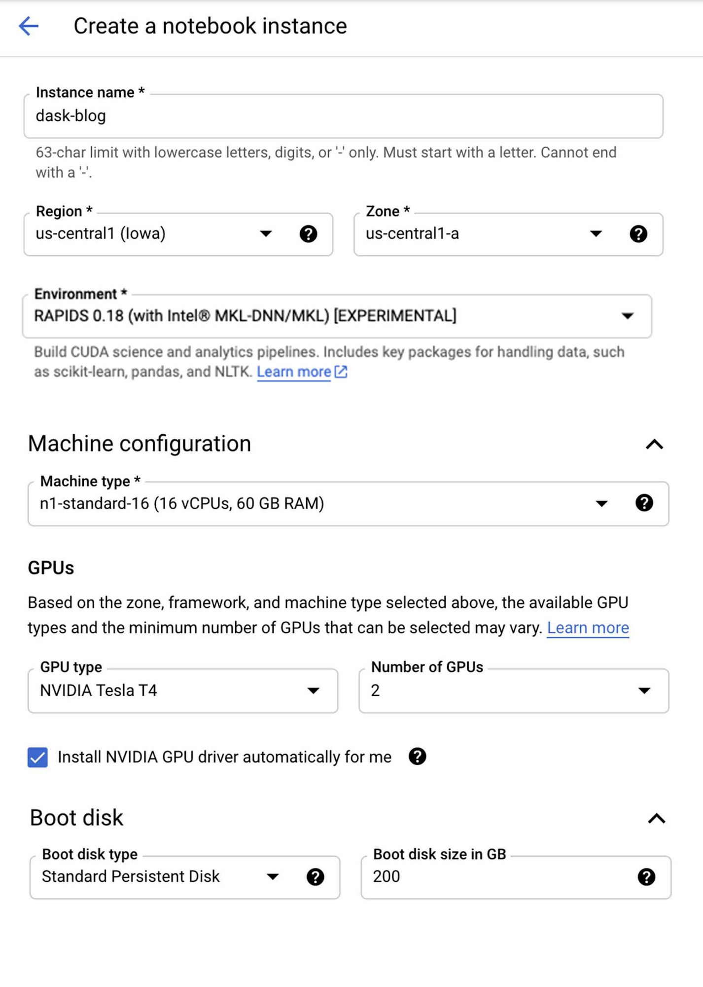
*Be sure to check the “install GPU driver” box or you will need to manually install it and restart your instance!
** If you will be using the AI Notebook instance to generate the Higgs dataset (instructions to come in later section), then upload it to the cloud, you will want to increase your boot disk size to 200GB.

Click “Create” to spin up your notebook environment. This will take a few minutes. Once it is finished, a button will appear next to your instance that reads “Open Jupyterlab”. Click this button to enter the Jupyterlab instance. 

Interacting with your AI Notebook

Most data scientists will be familiar with Jupyter Notebook functionality.  Because we chose the Rapids 0.18 image, which has been specially designed for using Rapids and Dask, we won’t need to install additional libraries. You can start coding immediately!

You can also issue terminal commands from within a Jupyter notebook. Select file > New > Notebook. Create a new code block, paste the following command in it, and execute it. This will clone the github repository for this tutorial into your Notebook instance. You can use the file navigator on the left of the Jupyter console to navigate through your folders and files. You can also manage  your own github repository from the Git page of the Jupyter console.

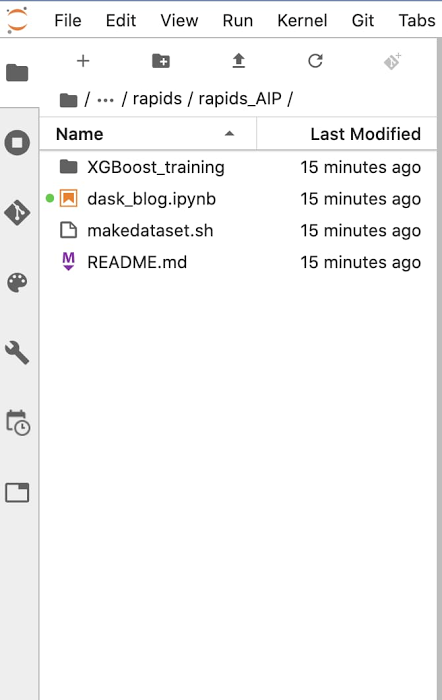
Navigate to ~/ai-platform-samples/training/rapids/rapids_AIP. This will be the folder where you will find all the files needed for this tutorial. Start by opening dask_blog.ipynb.

You can also install Dask into your local environment from scratch by following these instructions.

Instantiate LocalCudaCluster

Now we will instantiate a LocalCUDACluster, which will be used to assign the attached GPU to the Python processes. Note that it is not necessary to use Dask with a single node and a single GPU (cuDF and cuML will also work - and you can use more functions with those libraries), but we will need it once we scale up.

Prepare Data

The dataset we will be using for this tutorial is simulated particle activity data that was released for the Higgs Boson Machine Learning Challenge. We will be replicating this public dataset, and using different subsets of Higgs (some larger, some smaller) to demonstrate the scaling ability of Dask on AI Platform. 

Executing makedataset.sh script in the repo will download the dataset, replicate it, and upload it to GCS in the github. You can execute this script in your AI Notebook, or run it in a separate GCE instance, or run it locally if you wish.

There are many ways to ingest data into your Notebook instance, including uploading a local file. We will be reading the data from GCS (Google Cloud Storage), into a DataFrame that can be processed by GPUs.

cuDF is a Python GPU DataFrame library (built on the Apache Arrow columnar memory format) for loading, joining, aggregating, filtering, and otherwise manipulating tabular data using a DataFrame style API.

Dask-cuDF extends Dask where necessary to allow its DataFrame partitions to be processed by cuDF GPU DataFrames as opposed to Pandas DataFrames. For instance, when you call dask_cudf.read_csv(…), your cluster’s GPUs do the work of parsing the CSV file(s) with underlying cudf.read_csv().

For faster performance, you can use Parquet format instead of CSV. You will also need to shard your data so that it can be distributed across the workers. There are multiple ways to do this. You can partition your data into multiple files before reading it in, then use the * decorator to read them in. This is the route we will take in this tutorial. You can also use the npartitions argument with read_csv(), or chunk size in Dask Array to set the partitions.

A good rule of thumb is 1 GB partitions for an NVIDIA T4 GPU, and 2-3 GB is usually a good choice for a V100 GPU (with above 16GB of memory). Larger partitions will generally result in faster performance up to a point, but you need to be sure they will fit in your GPU memory.

This will read in our first dataset, and show the number of partitions. Our dataset is 10GB, with ten 1GB partitions.

Now we can execute some basic functions on the Dask Dataframe. This takes around a minute to run. As a note, this medium blog showed that these Dask functions execute 2-3x faster on GPUs than on CPUs. If you tried to do this group by on a pandas DataFrame of this size, your machine may very well error out, or take hours to complete the task.

You can keep track of your GPU’s memory usage by executing nvidia-smi dmon in the terminal, within the rapids-0.17 conda environment. For more metrics, you can utilize Jupyterlab extensions like dask-labextension or  nvdashboard , which will visualize various charts and metrics like GPU memory use and utilization. Using dask-labextension, we can see that GPU utilization is spiky. The “Dask Gpu Memory” total is inaccurate as it’s measuring the total memory of the localCUDAcluster, which includes the CPU memory of the notebook instance.

At present, using un-supported Jupyterlab extensions with AI Notebooks can be difficult (we’ve included instructions on how to do it in the git repo but there’s no guarantee that will work with other configurations). If this is a requirement, we recommend using Dask on GKE or Dataproc, and configuring your own Jupyter environment. In our next blog, we will explore how to visualize GPU metrics in greater detail.

Scale to 20GB

Now, we want to read in a 20 GB dataset, but our attached NVIDIA T4 GPU only has 16GB of memory. Luckily, Dask allows us to spill from GPU memory to host memory when the GPU runs out. To do this, we restart the Python kernel, and create a new LocalCUDACluster with a device_memory_limit set.  Dask will typically spill to disk by default, but setting device_memory_limit allows you to control when that will happen.

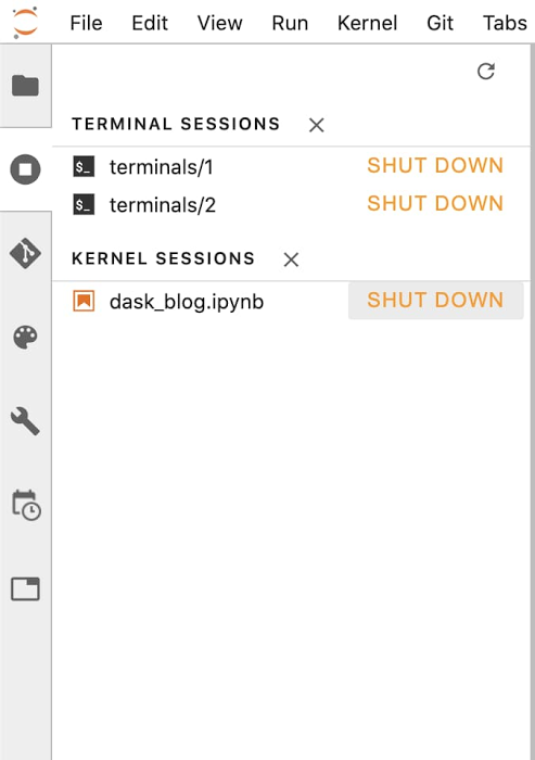
Note that you can instantiate a new LocalCUDACluster by shutting down and restarting the kernel using the terminal and kernel session control page in jupyterlab. Make sure you choose the rapids-0.17 kernel.

Execute the code again to run the functions. Dask manages the movement of the data so that it can execute despite the constraints. This takes ~2 minutes to execute.

Scale to 100GB using AI Platform Training

Now we would like to train an XGBoost model on our 100 GB dataset. However, even using Dask Dataframes, XGBoost executes completely in memory, meaning we can’t spill as dynamically from GPU to host memory. This means we need to beef up our GPUs.

Note that it is easy to resize your AI Notebook instance with more GPUs or GPUs of a different kind. However, we want to take a more dynamic approach by using AI Platform Training with custom containers. AI Platform Training will spin up the resources we specify, run our code as a job, then spin them down when completed. And, we can easily package and submit our code from AI Notebooks.

We will run the same libraries we used above, but on AI Platform Training with four NVIDIA A100 GPUs. A100s available in AI Platform have 40GB of GPU memory and you can scale up to 16 of them on a single machine without having to worry about multi-node distribution (As of the time this blog is published, GCP is the only Cloud Provider to support 16). This gives you a whopping 640GB GPU memory to play with. This both simplifies managing your environment and limits any networking issues that could pop up when dealing with multi-node setups.

Training with Containers

By using Containers, we can customize exactly how our training job is submitted, and on what machines. 

As you already cloned the entire Git repository, use the Jupyterlab navigation panel to navigate to the XGboost_training folder. Inside, you will find the files necessary to build the RAPIDS-based container, and deploy the AI Platform Training Job.

Build the container

You can see in the Dockerfile that we are using a base image from RAPIDS.

To build the container and push it to your own GCR, open build.sh and update the path to match your repository. Then execute the script.

XGBoost on AI Platform Training 

Open the rapids_dask.yaml file. This is how we configure the machines on which AI Platform Training will execute our XGBoost code. As you can see, we are using 4 GPUs of the type A100. See a full list of the GPUs available in each region, and with what machine types here.

Update the bracketed variables, and change the imageURI if you build your own container. Save the file when you are done.

Now we are ready to submit the training job. Do this by executing the following code in the AI Notebook terminal (also found in the README file).

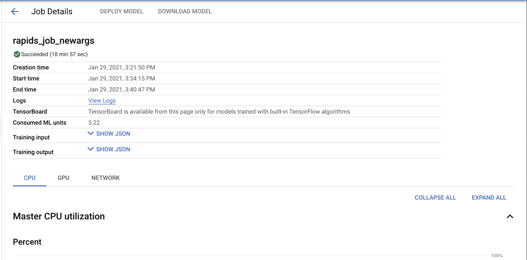
You can monitor your job by clicking on it from the list of jobs in AI Platform on Cloud Console (AI Platform > Jobs). On the job details page, you can see a variety of metrics, such as CPU and GPU utilization. In addition, you can click on the “View Logs” link to be taken to Cloud Logging, where you can see all logs generated by your job. Or, execute gcloud ai-platform jobs stream-logs $JOB_NAME to stream the logs in your terminal.

It will take around 11 minutes to spin up the training environment and begin executing the code. You can follow along with the steps by watching the logs. The usage metrics will take a few minutes to propagate as well. When we ran this job using a 100GB dataset, it completed in 19 minutes (including training environment spin up time), with the XGBoost training portion taking only 56 seconds!

By making a few minor changes to the YAML file, we can run the same code on 4 NVIDIA T4 GPUs. Dask recognizes that it cannot be executed completely in GPU memory, and therefore spills to disk when necessary. This results in an overall job time of 20 minutes, and a training time of 124 seconds. With 8 V100 GPUs, we saw a training time of 28 seconds! We encourage you to play around with different resource configurations and data sizes, as AI Platform makes it easy to do so.

Deploy Model for Online Prediction

Now that you have a trained model in your GCS bucket, you can deploy that model on AI Platform Predictions for online inference. Once again, you can leverage GPUs to increase the inference speed.

Clean Up

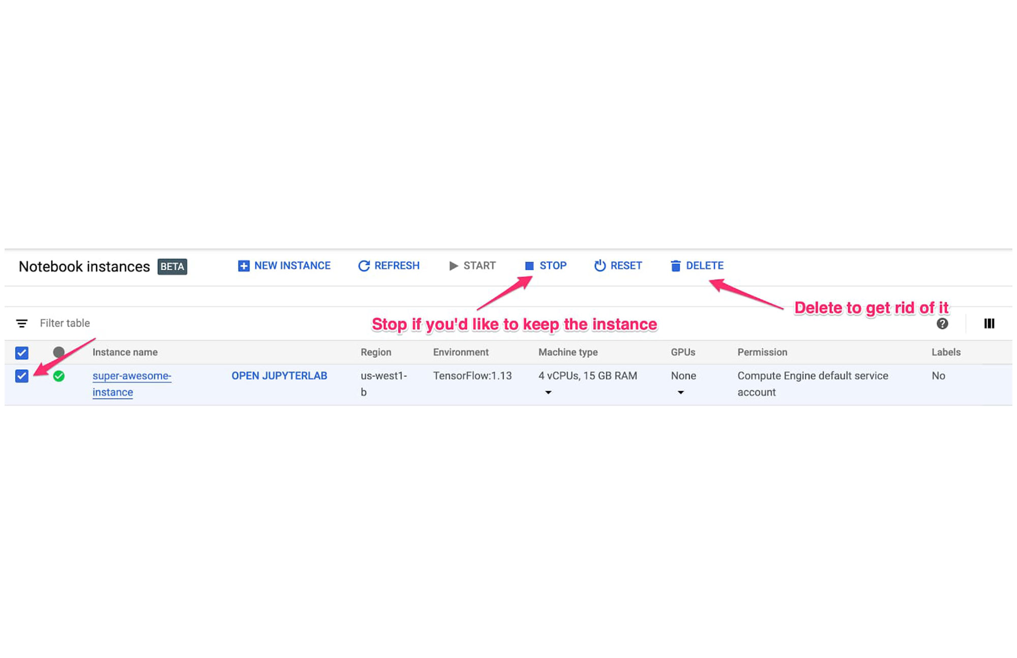
Delete the AI Notebook instance to prevent any further charges. If you want to save your work, you can choose to stop the instance instead.

Delete the GCS bucket.

Conclusion

Dask is an exciting framework that has seen tremendous growth over the past few years. RAPIDS + Dask allows you to leverage the power of NVIDIA GPUs, which can greatly decrease your data processing and training time. We saw that using NVIDIA A100 GPUs resulted in a lower training time compared to NVIDIA T4 GPUs, even with twice the data. 

Dask is also handy in its ability to automatically tailor its method of execution based on the resources you have available. We saw that Dask will automatically revert to using CPU memory when GPU memory is exhausted, and that you can control this mechanism. 

AI Platform allows you to quickly get started with Dask. You can develop in Jupyterlab with any number of GPUs in AI Notebook. You can then scale up your code to execute on souped-up machines on-demand with AI Platform Training. Imagine what you could do with 16 A100 GPUs at your disposal?  

Need more proof that NVIDIA GPUs can speed up your XGBoost training, check out this blog. Find out more fun ways to use A100s here.

^{Big thanks to Mikhail Chrestkha, Winston Chiang, Guoqing Xu, Ethem Can, Dong Meng, Arun Raman, Rajesh Thallam, Michael Thomas, Rajan Arora and Subhan Ali for educating me and helping with the example workflow.}