Projected Changes in Soil Temperature and Surface Energy Budget Components over the Alps and Northern Italy

Abstract

This study investigates the potential changes in surface energy budget components under certain future climate conditions over the Alps and Northern Italy. The regional climate scenarios are obtained though the Regional Climate Model version 3 (RegCM3) runs, based on a reference climate (1961–1990) and the future climate (2071–2100) via the A2 and B2 scenarios. The energy budget components are calculated by employing the University of Torino model of land Processes Interaction with Atmosphere (UTOPIA), and using the RegCM3 outputs as input data. Our results depict a significant change in the energy budget components during springtime over high-mountain areas, whereas the most relevant difference over the plain areas is the increase in latent heat flux and hence, evapotranspiration during summertime. The precedence of snow-melting season over the Alps is evidenced by the earlier increase in sensible heat flux. The annual mean number of warm and cold days is evaluated by analyzing the top-layer soil temperature and shows a large increment (slight reduction) of warm (cold) days. These changes at the end of this century could influence the regional radiative properties and energy cycles and thus, exert significant impacts on human life and general infrastructures.

1. Introduction

In recent years, the scientific community has recognized the importance of the land surface as a key component of the climate system [1,2,3]. The soil can be considered a lower boundary condition for the atmosphere, being a source term for the hydrologic and energy budgets in the atmospheric surface layer. Slightly different conditions of some crucial parameters, such as the soil moisture and temperature, can affect the stability of the boundary layer and, generally, of the whole troposphere. Atmospheric stability is a fundamental parameter related to convective motion, which rules the formation of clouds and precipitation that are very common in tropical areas.

The soil acts in two ways in the climate system. On one hand, it partitions the incoming net radiation (NR) into sensible heat flux (SHF) and latent heat flux (LHF) to the atmosphere and conductive heat flux (CHF) to the underground soil. On the other hand, it redistributes the income of water from precipitation into evapotranspiration (ET), surface or underground storage, runoff or gravitational drainage. Being proportional to ET, LHF is a key variable that links energy and hydrologic exchanges. For this reason, assessment of the soil hydrologic budget is crucial to allow correct evaluation of the energy budget components [4].

In spite of the importance of these physical variables in determining the soil surface properties and phenomena, only a few cases of extensive field campaigns have been carried out in order to measure soil temperature and moisture, or turbulent fluxes. In particular, compared to several soil moisture measurement programs (e.g., references [5,6,7,8,9,10,11]) there have been substantially fewer extensive measurements of soil temperature (ST)—mostly within local regions (e.g., references [12,13,14]). Despite the existence of several databases relevant to surface soil (skin) temperature, mostly based on satellite products (e.g., [15,16,17]), the lack of observational data on ST profiles, especially in the root layer zone, makes it very difficult to evaluate the land surface energy budgets for wide areas and over a suitably long period of time. To avoid this data deficiency, an alternative method has been proposed: Numerical model outputs are used as a surrogate of surface observations to estimate, on a mesoscale area, the thermal and hydrologic state of the soil, its exchanges of energy and moisture with the atmosphere, and the soil temperature and moisture. This technique, called the CLImatology of Parameters at the Surface (CLIPS) [18], is based on the output of a trusted land surface model (LSM) carried out over some meteorological stations. Such LSM is usually driven by standard observations of the stations, such as temperature, pressure, humidity, precipitation, wind intensity, and solar radiation. Examples of similar applications can be found in several previous studies (e.g., references [19,20,21,22,23]). The model-generated ST products have proved to be generally in good agreement with observations and have often served as alternatives for observations (e.g., references [24,25,26,27,28,29,30]) . Recently, land surface parameters in LSMs have been obtained more accurately via scheme optimization (e.g., references [31,32]) and/or parameterization improvement (e.g., references [33,34]).

In this study, we investigate the potential changes in the Alps and Northern Italy near the end of this century (i.e., 2071–2100) discriminatively over high-mountain versus plain areas from the viewpoint of land surface energy budget components. There have been many studies on the projected changes over Europe, including in our study areas, based on future climate change scenarios (e.g., references [35,36,37,38,39]);however, discussions on regional changes in terms of detailed analyses on land surface energy components have seldom been made. We apply the CLIPS method to drive the LSM using climate model outputs instead of meteorological observations. Moreover, the time span used is sufficiently long (30 years) in order to make a climatological analysis of the results possible. Section 2 describes the models used in this study, and Section 3 introduces the experiment design and methods. Results and discussions concerning the energy budget are reported in Section 3, and conclusions are given in Section 4.

2. Model Description

For the climate model and LSM in this study, we employed the Regional Climate Model version 3 (RegCM3) [40] and the University of Torino model of land Processes Interaction with Atmosphere (UTOPIA) [41], respectively.

The RegCM3 has participated in several important multi-model ensemble projects, including the European Union project, called the Prediction of Regional scenarios and Uncertainties for Defining EuropeaN Climate change risks and Effects (PRUDENCE; see http://prudence.dmi.dk/), the Central and Eastern Europe Climate change Impact and vulnerabiLIty Assessment (CECILIA; http://www.cecilia-eu.org/), and ENSEMBLES (http://ensembles-eu.metoffice.com/). Although a product from a newer version of RegCM (i.e., RegCM4) is available for Europe within the Coordinated Regional Downscaling Experiment (EURO-CORDEX; http://www.euro-cordex.net/), we selected the RegCM3 output because it is one of the existing high-resolution datasets currently available (20 km) and has been used in numerous previous studies on climate projections, especially over Europe and the region of this study (i.e., the Alps and plain Po Valley areas), even until most recently (e.g., references [35,36,37,38,39,42,43,44,45,46,47,48]). The RegCM model was able to simulate the surface solar radiation patterns over Europe [49], with smaller biases over land at the surface [50]. Despite these considerations being based on version 4 of RegCM, whereas we used version 3, the radiation parameterization has not changed through the version upgrade [51], and the two versions have not shown significant differences in energy budget components [52].

The UTOPIA, formerly called the Land Surface Process Model (LSPM) [53,54], is a one-dimensional diagnostic model, based on the soil–vegetation–atmosphere transfer (SVAT) scheme that was originally developed by [55]—see the reviews on the SVAT scheme in [56,57]. In UTOPIA, variables are mainly diagnosed in the soil and vegetation layers. The soil state is described by its temperature and moisture content, which are calculated by integrating the heat Fourier equation and the water mass conservation equation using a multi-layer scheme. The UTOPIA has been widely used for studies of energy/hydrologic cycles and atmosphere–land surface interactions over the domain of our study, especially over the Alps, Po Valley and Piemonte, Italy (e.g., references [22,54,58,59,60,61,62]), and other regions outside of Europe (e.g., references [23,30,63,64,65,66]).

The UTOPIA quantifies the exchanges of energy, momentum, and water between the atmosphere and land surface through three main zones: The soil, vegetation, and atmospheric layers. It calculates the land surface energy and hydrologic budgets in terms of physical fluxes and the hydrologic state of the land: the former includes fluxes of radiation, momentum and sensible and latent energy, and heat transfer in multi-layer soil, whereas the latter includes rainfall, snow melt and accumulation, interception, infiltration, runoff, and soil hydrology. The surface energy budget is evaluated considering all vegetation fluxes (i.e., radiative, conductive, and convective fluxes), bare soil and snow, in which the weights are determined by the respective fractional covers.

We note that UTOPIA possibly contains its own model error as all other models do. The model error can be evaluated by taking the difference between the model results and their corresponding observations. From previous comparisons with data from a field experiment, the root mean square error of the UTOPIA simulations for the energy budget components is around 50 W m${}^{-2}$, which can be considered to be a typical model error of UTOPIA. This is comparable to the typical errors of about 30–50 W m${}^{-2}$ for radiation measurements. The biggest assumption made by UTOPIA is that the energy budget is closed; thus, net radiation and sensible and latent heat fluxes are calculated and soil heat flux is evaluated by the closure of the budget. Since RegCM3 is based on BATS-1e, its energy budget is also closed.

3. Experiment Design and Methods

Most previous studies have driven the LSM used in CLIPS with meteorological observations (e.g., references [21,22,23]). Most recently, Park et al. [30] used the output of a regional climate model (RCM) as input data for CLIPS. As we aim to evaluate the climate change effects on the energy budget components, we also used the RCM output, instead of the station observations, to drive the LSM. Currently, horizontal resolutions of some RCMs are around 10 km (e.g., references [67,68,69,70,71]). This is sufficiently high to infer the general characteristics of the energy and hydrologic cycles for large and medium scale basins, though still quite coarse to allow the energy budget components in a small scale basin to be detailed (e.g., references [69,70]).

In this study, we used the output from RegCM3 to derive meteorological input data for UTOPIA. In more detail, UTOPIA was driven over each grid point using the following RegCM3 outputs: Longwave and shortwave radiation, precipitation, and the surface-level (2 m) temperature, humidity, pressure, and wind. To ensure the numerical stability of UTOPIA, all 3-hourly RegCM3 non-intermittent outputs were interpolated every hour using a cubic spline, whereas the intermittent variable, e.g., precipitation, was simply redistributed assuming a constant rate (see more details in [4]).

For the UTOPIA simulations, we set a total of 10 soil layers with a total soil depth of ∼51 m. The soil thickness of the surface layer was 0.05 m, and then it increases exponentially to the lowest layer (∼25 m), which is regarded as a boundary relaxation zone. More specifically, we set the bottom-level depth, from layer 1 (top) to layer 10 (bottom), to 0.05, 0.15, 0.35, 0.75, 1.55, 3.15, 6.35, 12.75, 25.55, and 51.15 m. Here, the deepest layers near the bottom are intended for the boundary relaxation zones, as described in reference [4]. Despite UTOPIA possessing an internal algorithm for dealing with a non-null heat flux from the bottom, there is no similar algorithm for dealing with eventual (non-null) moisture fluxes. Since moisture values influence soil heat flux, we preferred to take very deep soils in order to prevent non-null (i.e., spurious) fluxes of heat and moisture from the bottom. This allowed us to minimize errors in the initial soil temperature and soil moisture values in UTOPIA, which are obtained through analytical solutions [41], without using any soil data from the RegCM3 soil scheme—Biosphere–Atmosphere Transfer Scheme (BATS) version 1e [72]. The e-folding depth of a thermal wave, considering the loam soil, is close to 5 m; thus, the total soil depth of only about 4–5 m, used in most soil models (including BATS), is insufficient to represent the propagation of energy and water into soil for a climatic time span. Therefore, having a deep relaxation layer can minimize the effect of approximating null moisture flux at the bottom, at the expense of computational time.

We obtained the soil characteristics data from ECOCLIMAP soil texture [73,74], and used the same data for all soil profiles due to the absence of other sources of data regarding deep soil composition. In terms of vegetation, we assumed that short grasses cover the whole domain, in accordance with [4], though the tree line elevation in the Swiss Alps can reach up to 2450 m [75,76] with various types of vegetation. This assumption, i.e., having short grasses over all the domain grid points, is based on the following considerations, mainly associated with the large uncertainty in projection of future vegetation aspects: (i) RegCM3 had no dynamic vegetation parametrization and employed fixed vegetation and land use data; (ii) the grid resolution of RegCM3 was not sufficient to represent the detailed orographic features, and hence, the changes in natural vegetation and land use exerted by potential climatic variability; (iii) most hilly and plain areas are extensively used for agriculture and are subject to irrigation and thus, it is hard to predict the vegetation aspects by models based on the natural vegetation change; and (iv) vegetation dynamics are conditioned by not only climatic factors but also by artificial factors (e.g., adaptive ecosystem management [77]).

We further note that short grasses can be roughly considered common cereals or such kind of agricultural products (except C4 crops, such as maize), of which the majority do not exert substantial impacts on energy and water balance with regard to plant height, root depth, and vegetation characteristics; thus, we decided to use a homogeneous plant cover over the entire domain in order to obtain signals that were not biased by the vegetation variation but that were dependent exclusively on the climate change projected by RegCM3.

For the analyses of the energy budget components, we considered three 30-year (normal) periods: The reference period, 1961–1990 (hereafter referred to as the reference climate, or RC), and the last thirty years of the 21st century (2071–2100), referred to as the future climate (FC). FC${}_{A2}$ and FC${}_{B2}$ were projected through the A2 and B2 emission scenarios, respectively, from the Intergovernmental Panel on Climate Change (IPCC) Special Report on Emissions Scenarios (SRES) [78]. The analyses of the hydrologic budget components (including soil moisture, dry and wet soil indices, and snow) over the same domain and periods of our study are conducted in reference [4]. Although climate change due to anthropogenic or climate-induced sources, e.g., land-use/land-cover change, biofuel expansion and vegetation migration, have been addressed recently (e.g., references [79,80,81]), we focused on the climate projections based on the SRES A2 and B2 scenarios only.

As the climate projections in this study were based on a single-model approach, we acknowledge quite large potential uncertainty in the projected changes related to model bias and ensemble variability. We employed the single-model approach due to limitations in resources to conduct ensemble simulations using multiple models and/or initial conditions. Under such limited conditions, the single-model approach with high resolution is often an alternative choice to the ensemble approach with coarse resolution, especially over complex terrain. For example, Coppola and Giorgi made high-resolution (20 km) RegCM3 simulations and found that the projected changes in both temperature and precipitation were in accordance with the ensemble results [45]. Although the single-model approach has been adopted in many previous studies on various climate change impacts/projections (e.g., references [30,35,82,83], etc.), an ensemble approach is more desirable for the estimation of a possible range of climate projections.

We calculated the energy budget components based on the energy balance at the land surface as follows:

$$R_{S\downarrow }+R_{L\downarrow }=R_{S\uparrow }+R_{L\uparrow }+H_S+H_L+H_C,$$

(1)

where $R_S$ and $R_L$ mean the shortwave and longwave radiation, respectively, and the downward and upward arrows imply the incoming and outgoing directions, respectively. $H_S$ is SHF, $H_L$ is LHF, and $H_C$ is CHF to the soil. This can be alternatively expressed in terms of the net radiation (NR), $R_N$, as

$$R_N=(1-\alpha )R_{S\downarrow }+\epsilon (R_{L\downarrow }-\sigma T^4)=H_S+H_L+H_C,$$

(2)

where $\alpha$ is the surface albedo, $\epsilon$ is the surface emissivity, $\sigma$ is the Stefan–Boltzmann constant, and T is the Earth’s radiating temperature. Therefore, $(1-\alpha )R_{S\downarrow }$ means the net shortwave radiation, and $\epsilon (R_{L\downarrow }-\sigma T^4)$ the net longwave radiation.

We made preliminary comparison experiments (not shown) for heat fluxes in the RC between UTOPIA and RegCM3 that were coupled with the BATS soil scheme [72]. In the plain area, SHF from RegCM3 was significantly larger than that from UTOPIA in summer (June–September); LHF from RegCM3 was always larger than that from UTOPIA except in July and August when both results became similar. We believe that this behavior is mainly due to the differences in soil water transfer parameterization, i.e., the force-restore method in BATS versus the diffusion approach in UTOPIA, as discussed in [20]. The exceptionally large SHF from RegCM3 in summer was mainly because evapotranspiration decreased when soil moisture became too low—a known problem of the force-restore method [20]. Therefore, the Bowen ratio (i.e., the ratio of SHF to LHF) for RegCM3 appeared larger than unity in July and August, and lower than unity in other months; on the contrary, for UTOPIA, the Bowen ratio was close to unity throughout the whole year. In the high mountains, UTOPIA simulated a null LHF from November to May when snow covered the area, whereas RegCM3 produced appreciably positive LHF for the same period; LHF from UTOPIA was more reasonable because the surface temperature is 0 ${}^{\circ }$C with snow cover, and hence, transpiration is null. The Bowen ratio from June to October (i.e., for the months with non-null LHF in UTOPIA) was close to unity for UTOPIA, while much larger than unity for RegCM3. Furthermore, SHF from RegCM3 was slightly positive from March to May, indicating that some points in the high mountains (>2500 m) were not covered by snow. In reality, however, all areas at such high elevations were fully covered by snow from March–May, except in very unusually snowless winters. Therefore, we believe that UTOPIA shows more realistic and reasonable results than RegCM3 in terms of the energy budget components. We further note that more direct and meaningful comparisons can be made by using either coupled models (i.e., RegCM3-UTOPIA and RegCM3-BATS) or offline models (i.e., UTOPIA and BATS).

We also investigated the occurrence of warm and cold days using the surface STs diagnosed by UTOPIA instead of employing the air temperature data from RegCM3. Generally ST is more stable with less fluctuations than air temperature. Various studies have indicated that using ST instead of air temperature in early growth stages provides greater accuracy for predicting crop phenology and growth [84,85], which eventually affects various land surface processes afterwards, including air temperature. In calculating ST, UTOPIA considers the freeze–thaw dynamics and its related physical processes, while RegCM3 does not. Taking these factors into account, we believe that more reliable warm/cold days occurrence can be evaluated using ST (from UTOPIA) than air temperature (from RegCM3).

In defining the warm and cold days, we considered two thresholds in the daily mean ST of the surface soil layer: (i) An upper threshold (30 ${}^{\circ }$C) for warm days and (ii) a lower threshold (0 ${}^{\circ }$C) for cold days. These thresholds were carefully chosen by primarily considering their effects of on vegetation, because ST is the main factor responsible for a decline in root biomass and the vegetation regeneration rate [86]. The value of 0 ${}^{\circ }$C in the root zone is harmful for some cultivations (no vascular plant can grow below 0 ${}^{\circ }$C)—for several plants, temperatures below 0 ${}^{\circ }$C force the accumulation of chilling units to prevent premature budding in the subsequent spring [87]. On the other hand, for most plants under conditions of an ST above 30 ${}^{\circ }$C, the canopy resistance tends to become very high, thus limiting the transpiration and production or affecting the pollen viability [88].

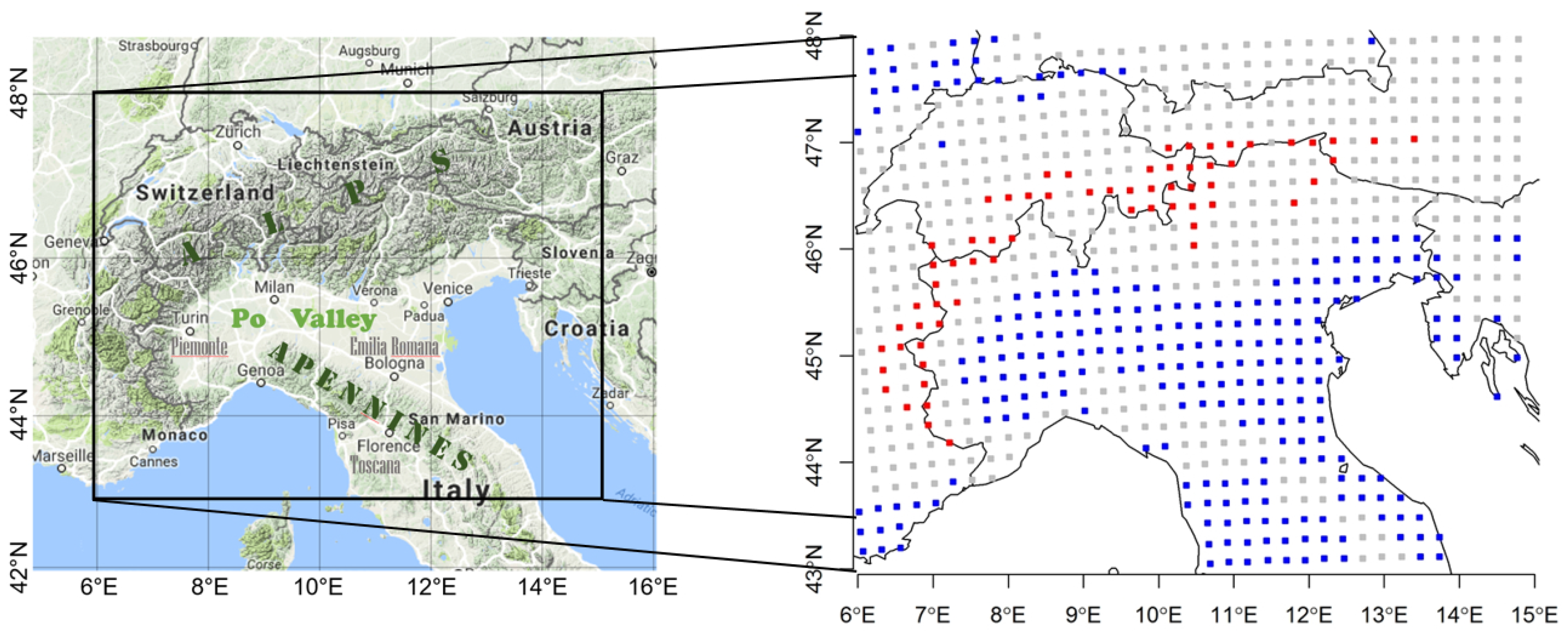
Figure 1 shows the computational domain, which occupies most of the Alpine region and Northern Italy, including the Po River basin, bordered by 5${}^{\circ }$ E–15${}^{\circ }$ E and 43${}^{\circ }$ N–48${}^{\circ }$ N. In this domain, a total of 720 grid points are defined which are categorized into three different areas depending on the grid elevation (h) above sea level (a.s.l.): the plain area (blue; h≤ 500 m a.s.l.), the normal-mountain area (grey; 500 m a.s.l. <h≤ 2000 m a.s.l.), and the high-mountain area (red; h> 2000 m a.s.l.).

4. Results

The results are shown here in two different ways. First, time trends of the 10-day mean values of some variables are presented for selected grid points to examine the temporal variability of the data. Second, the mean values of variables in some specific periods are shown in two-dimensional maps to show the spatial variability of the data.

4.1. Annual Mean Energy Budget in Orographically Relevant Areas

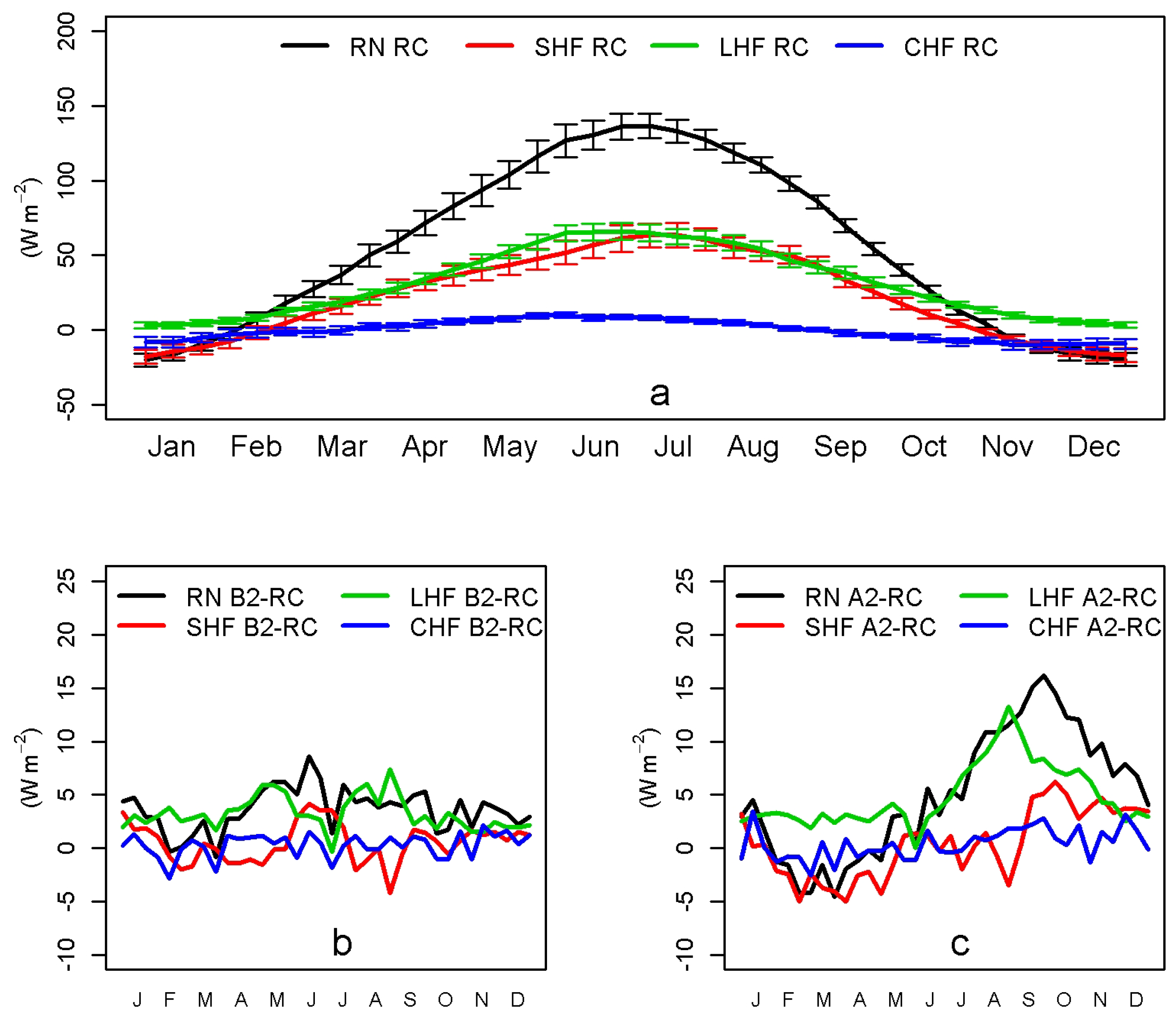
For the analysis of the annual mean energy budget, we discuss the results in terms of two grid-point sets—plains and high mountains (blue and red grid points, respectively, in Figure 1). The annual cycles of the energy budget components are evaluated, through the 10-day averages over the 30-year simulation period, at each grid-point set.

Figure 2 and Figure 3 show the annual cycles of energy budget components in the RC and the corresponding differences against FCs. For example, the LHF difference ($\Delta$LHF) represents LHF${}_{FC}$ minus LHF${}_{RC}$, where FC is either FC${}_{B2}$ or FC${}_{A2}$—similar to $\Delta$SHF, $\Delta$CHF, and $\Delta$NR. This is to emphasize the magnitude and direction of change in future energy budget components, since general trends of annual cycles are similar among the RC and FCs. Note that, for the RC, we also plotted the standard deviation of the energy budget components, averaged on all grid points and over each 10-day period (see Figure 2a and Figure 3a). The values and patterns in standard deviation for FCs were similar to those for the RC (not shown but referred to Figure 4), and the standard deviation values for the difference fields (i.e., FC${}_{A2}-$RC and FC${}_{B2}-$RC) were too large and less meaningful (not shown).

On the plains, for the RC, LHF slightly exceeds SHF in all months, except for summer when the two fluxes are almost equal (Figure 2a). This means that sufficient water usually exists in the soil for ET, whereas the available soil water content slightly decreases in summer due to the scarcity of rainfall—characteristic of the summer climate in Northern Italy. Autumn precipitation, however, restores this temporary deficit.

Figure 2b,c show the difference fields between the RC and FCs. $\Delta$LHF tends to exceed $\Delta$SHF in FCs, with the largest LHF increments observed in FC${}_{A2}$ between July and October (Figure 2c). The peak of LHF shifted from the beginning of June in the RC to July in both FC${}_{B2}$ and FC${}_{A2}$, whereas the peak of SHF was always at the end of June in phase with that of NR (not shown). This is caused by the noticeable increment in LHF, especially in summer, which masks the smaller increment in the SHF.

The increase of LHF in FCs is related to the increase in precipitation during the winter (e.g., [37]) which provides abundant soil moisture for evaporation during the spring and the beginning of the successive summer. On the other hand, the increase in LHF makes the soil drier during the summertime, confirming the results of reference [89].

The largest difference between FC${}_{B2}$ and FC${}_{A2}$ emerges from August to November, especially in $\Delta$NR and $\Delta$LHF (see Figure 2b,c). The peak of $\Delta$NR in FC${}_{A2}$ occurs in mid-September (nearly 20 W m${}^{-2}$) while that of $\Delta$LHF appears earlier, at the end of August, possibly because the soil moisture content approaches the wilting point—i.e., less available soil water content for evapotranspiration. A positive $\Delta$SHF is also observed in FC${}_{A2}$ during autumn and winter, which implies an increase in ST. In general, albedo (i.e., the reflected shortwave radiation) enhances as soil moisture decreases, and the upward longwave radiation augments as ST increases. The strongly positive $\Delta$NR in FC${}_{A2}$, despite the increase in ST and the decrease in soil moisture, can be explained by a less cloudy sky. Meanwhile, as soil moisture approaches the wilting point, vegetation suffers from hydraulic stresses and turns more yellowish, thus increasing its albedo.

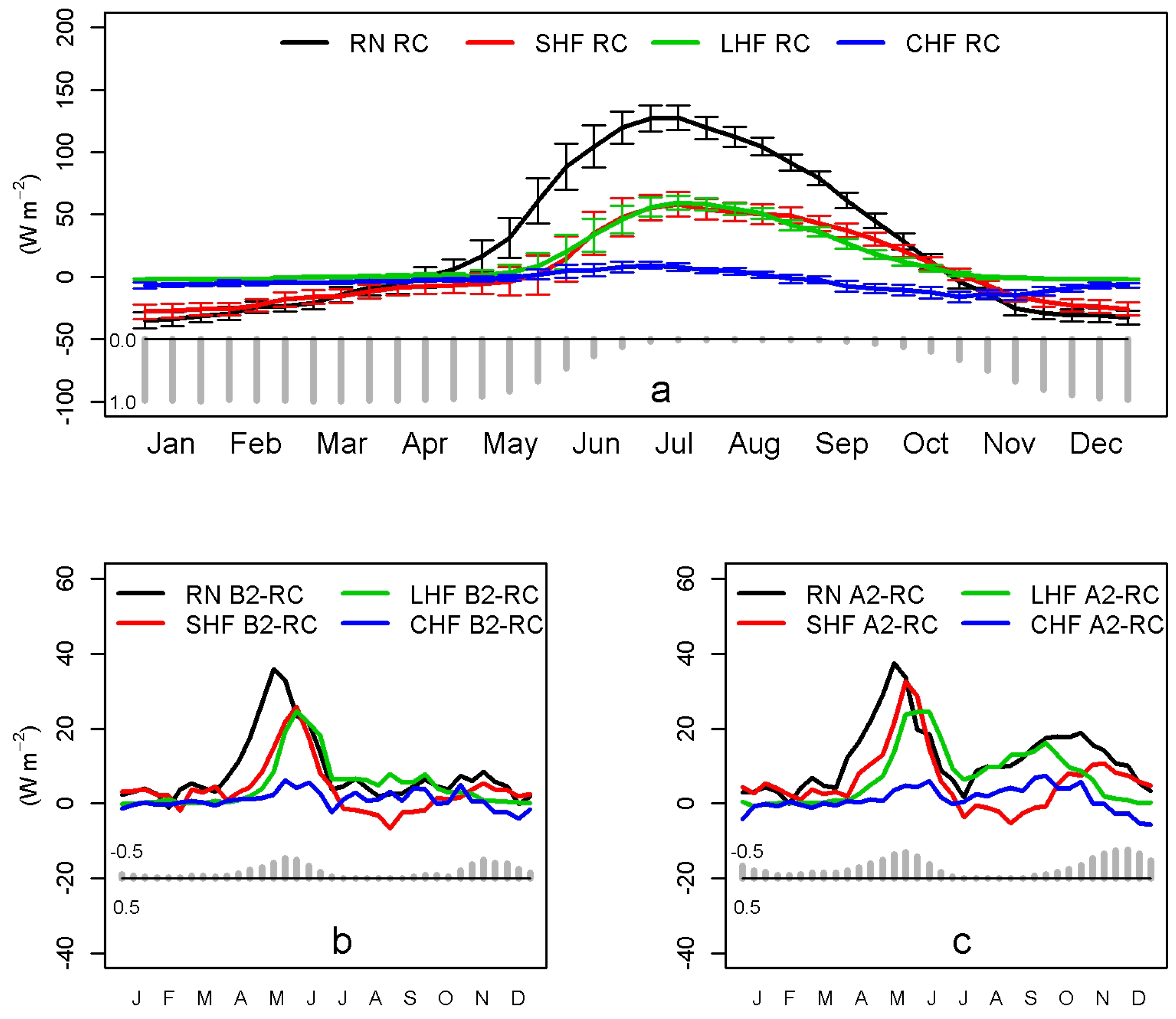
Figure 3 represents the energy budget components for the RC and FCs at high-mountain grid points. It is notable that the positive periods for all components at high mountains (Figure 3a) are much shorter than those on the plains (cf. Figure 2a) in the RC, and similarly to FCs (not shown). For example, in the RC, NR at high mountains is positive from mid-April to late October (for ∼6.5 months), while NR on the plains is positive from early February to early November (for ∼9 months); the positive SHF at high mountains appears from late May to the end of October, while that on the plains occurs from mid-February to early November. This is related to the presence of snow that begins to accumulate from late September, reaches its maximum at late December, and then gradually decreases from mid-May, and almost disappears by mid-July (see Figure 3a; grey bars). Snow significantly increases surface albedo and hence, decreases NR, thus lowering the soil heating and depleting LHF. It is evident that, in the high mountains, turbulent exchanges of energy occur mainly from late spring to early autumn.

In the RC, in the high mountains (Figure 3a), during spring and the latter half of summer, SHF and LHF show similar values; during late spring and in autumn, SHF is slightly higher than LHF. From late autumn to early spring, due to snow coverage over the soil, SHF is negative, while CHF and LHF are almost zero; consequently, NR is balanced mainly by SHF (i.e., both are similar in sign and magnitude).

The snow differences between FCs and the RC (say, $\Delta$SN) are negative in the high mountains, prominently during March–June and October–January, with larger magnitudes in FC${}_{A2}$ than in FC${}_{B2}$ (see Figure 3b,c; grey bars). This implies earlier disappearance and/or smaller amount of snow in FCs (see also Figure 6). Using ensembles of regional climate models, Coppola et al. [90] showed similar future snow variation in the Alps region. Our results indicate that all of the energy budget components in the high mountains in FCs are strongly controlled with the variation in $\Delta$SN; however, their behaviors are quite different for different seasonal periods of negative $\Delta$SN.

During the melting season, snows disappear earlier in both FCs; thus, STs start to increase as early as late March (see Figure 4b). The maxima of $\Delta$NR (∼36 W m${}^{-2}$) appear in mid-May in both FCs, whereas those of $\Delta$SHF (∼22 W m${}^{-2}$ in FC${}_{B2}$; ∼30 W m${}^{-2}$ in FC${}_{A2}$) arise around late May—In phase with the negative $\Delta$SN. Similar peak values of $\Delta$LHF (∼22 W m${}^{-2}$) are shown in both FCs, with a longer peak period in FC${}_{A2}$. Since snows disappear early and the FCs of the snow covered areas in the high mountains decrease , the surface albedos decrease, thus soil and vegetation receive more shortwave radiation. Therefore, NRs show large positive increments starting from late March. As the soil becomes wet due to snow melting, evaporation can occur and LHF shows a significant positive increment.

During the accumulation season, the snowfall amount is much less in FCs than in the RC, resulting in negative $\Delta$SN. In FC${}_{B2}$, $\Delta$NR and $\Delta$SHF are slightly positive, $\Delta$LHF is nearly zero, and $\Delta$CHF is slightly negative as a consequence of negative $\Delta$SN. This trend is the same in FC${}_{A2}$, but with much larger magnitudes in $\Delta$NR, $\Delta$SHF and $\Delta$CHF. In particular, $\Delta$LHF is strongly positive in FC${}_{A2}$ up to mid-November with a second maximum (∼16 W m${}^{-2}$) in late September—right after the snow accumulation starts—suggesting sufficient availability of moisture from soil and/or plants for evapotranspiration. In contrast, $\Delta$SHFs are negative during July–September in both FCs. Note that $\Delta$CHFs are positive during the same period, indicating that the ground temperatures at high mountains in FCs are higher than those in the RC. Therefore, given that SHF depends on both the ground temperature and the surface air temperature, the negative $\Delta$SHF implies much lower surface air temperatures in the high mountains in FCs.

Figure 4 shows the temporal variation in the 10-day average STs in the upper soil layer (5 cm deep) at the grid points of plains and high mountains. The standard deviations are also plotted for the RC and FCs. On the plains (Figure 4a), STs in FCs increase in all months. The largest increments (5–7 ${}^{\circ }$C) are observed in FC${}_{A2}$ during August–December, with relatively lower increments (2–3 ${}^{\circ }$C) in FC${}_{B2}$ during June–December. In addition, compared to RC, the warmest period is extended by ∼10 days in FC${}_{B2}$ and by ∼30 days in FC${}_{A2}$. In the high mountains (Figure 4b), the increment of STs in FCs is limited to April–November. This is caused by the snow cover effect, which brings about earlier warming of soil by about a month (30–40 days) in both FCs.

4.2. Temperature during the Snow Melting Season

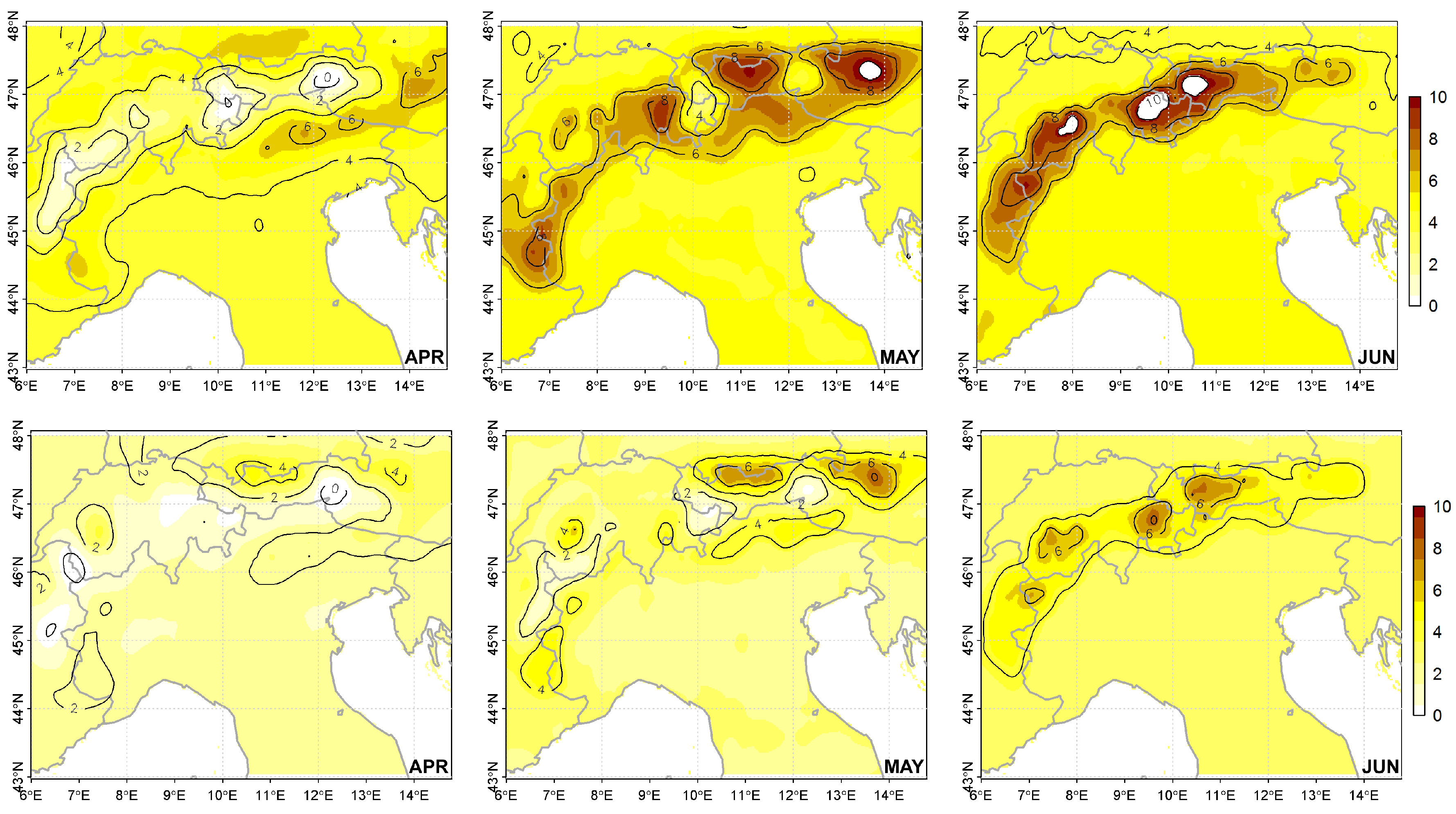
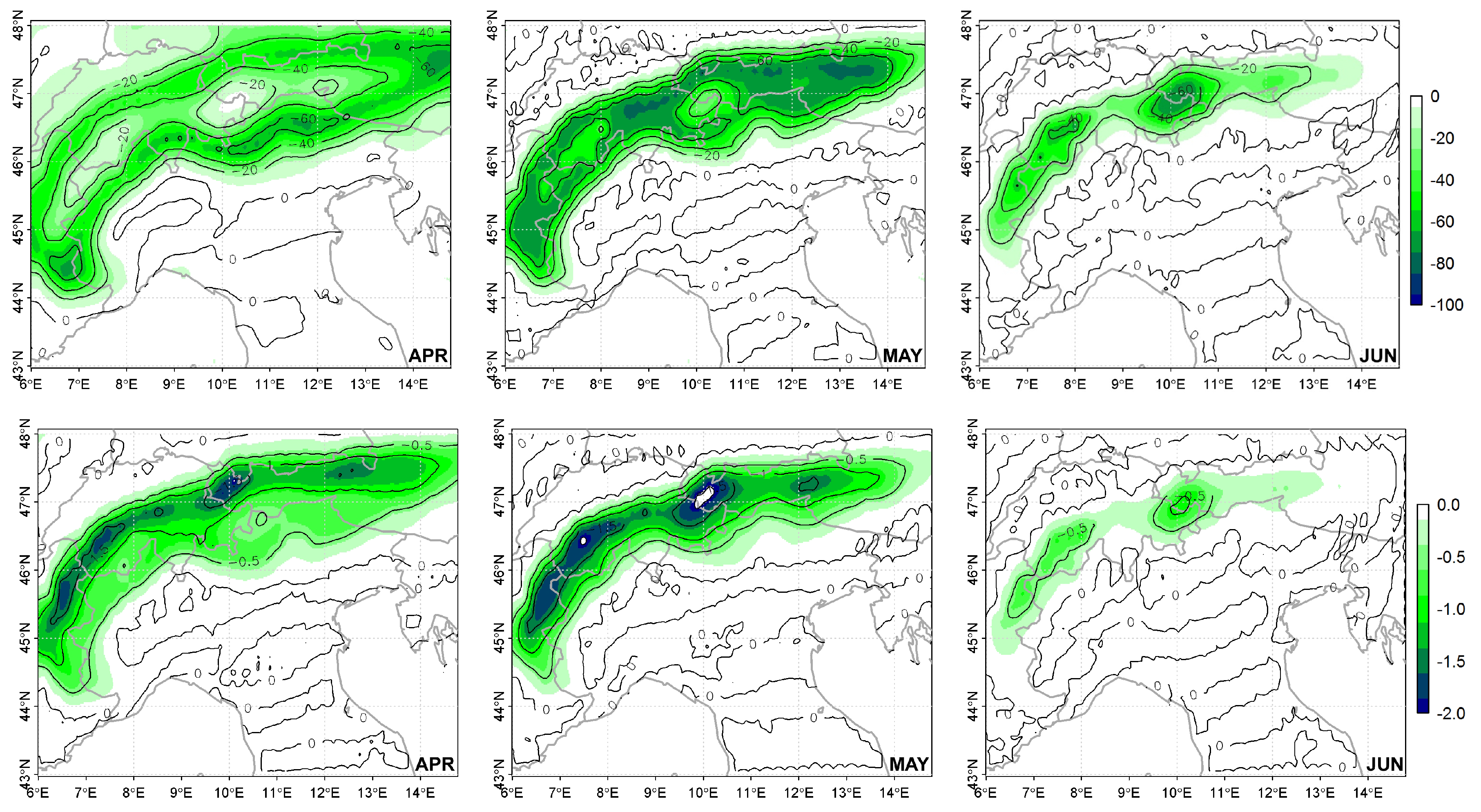
Figure 5 shows the difference in the ST ($\Delta$ST) in the surface soil layer (0–5 cm) between FC${}_{A2}$ and RC in April, Maym and June when $\Delta$STs are significantly large and non-uniform. Henceforth, we show the analysis results for all other fields only for these three monthsm because all other months had a general and almost uniform warming over the whole domain—Even negligible warming in July–September. In general, FC${}_{A2}$ shows larger anomalies thanm but similar patterns tom FC${}_{B2}$, and this is common to all other energy budget components; thus, hereafter, we depict and discuss the analysis results of other components for FC${}_{A2}$ only. In April, positive values of $\Delta$ST (i.e., warmer ST in FC${}_{A2}$ than in RC) appear over almost the whole domain, except in the alpine regions. The largest $\Delta$STs are located over the off-alpine regions, mainly on the Southern sides of the Alps, i.e., the zones most affected by the melting of premature snowpack; over the highest mountains, $\Delta$STs are much smaller or even slightly negative, indicating the persistence of the snow cover with a soil temperature near 0 ${}^{\circ }$C. In May, $\Delta$STs are positive everywhere with the largest values extending to the areas near the mountain peaks. In FCs, snow cover has already disappeared and soil surface warms earlier, thus showing a positive anomaly of temperature with respect to RC. A similar behavior is observed in June in the highest peaks of the Alps, potentially indicating free of snow in FCs while full of snow in RC therein.

We can directly relate this characteristic behavior of ST to the changes in snow cover and depth in FC${}_{A2}$. Figure 6 depicts the differences in snow cover and depth between FC${}_{A2}$ and RC. With regard to snow cover, in April, the off-alpine areas (i.e., middle-slope and/or foot) are affected by a large snow cover deficit; in May the largest snow cover deficit extends to the areas near the mountain peaks, whereas in June it appears only over the highest peaks. The lack of snow cover in these months justifies the ST differences (see Figure 5) and is consistent with the flux distribution observed in high mountains (see Figure 3), thus indicating the earlier seasonal growth of NR, SHF, and LHF by about one month in FC${}_{A2}$, due to the earlier snowmelt (with values close or even larger than 2 m in April and May). It is noteworthy that these features appear more prominently on the Southern and Eastern sides of the Alps, implying the potential for the most serious snow cover deficit in FCs in those areas. As far as snow depth is concerned, the areas of larger snow depth deficit shift to the north with the maximum in the Northern parts of the Alps, mostly ranging over France, Switzerland, and Austria in both April and May. Note that far more glaciers are spread over the Northern slopes than over the Southern sides of the Alps due to the year-round higher amount of solar radiation in the south and the larger accumulation of snow via wintertime humid air transport to the north. This implies the acceleration of melting and retreat of the Alpine glaciers in the Northern sectors of the Alps in FCs. The snow depth deficits tend to decrease approaching June because snow in FC${}_{A2}$ has already disappeared by that time.

Our results attest that the warmer conditions of FCs affect the starting time of snowmelt— antedating by about a month (30–40 days) in FC${}_{A2}$. This is consistent with the earlier increase in ST for the high-mountain area (see Figure 4b). This earlier snowmelt explains why, in FC${}_{A2}$, snow has already disappeared in the off-alpine areas in April and over the mountain peaks in May, respectively.

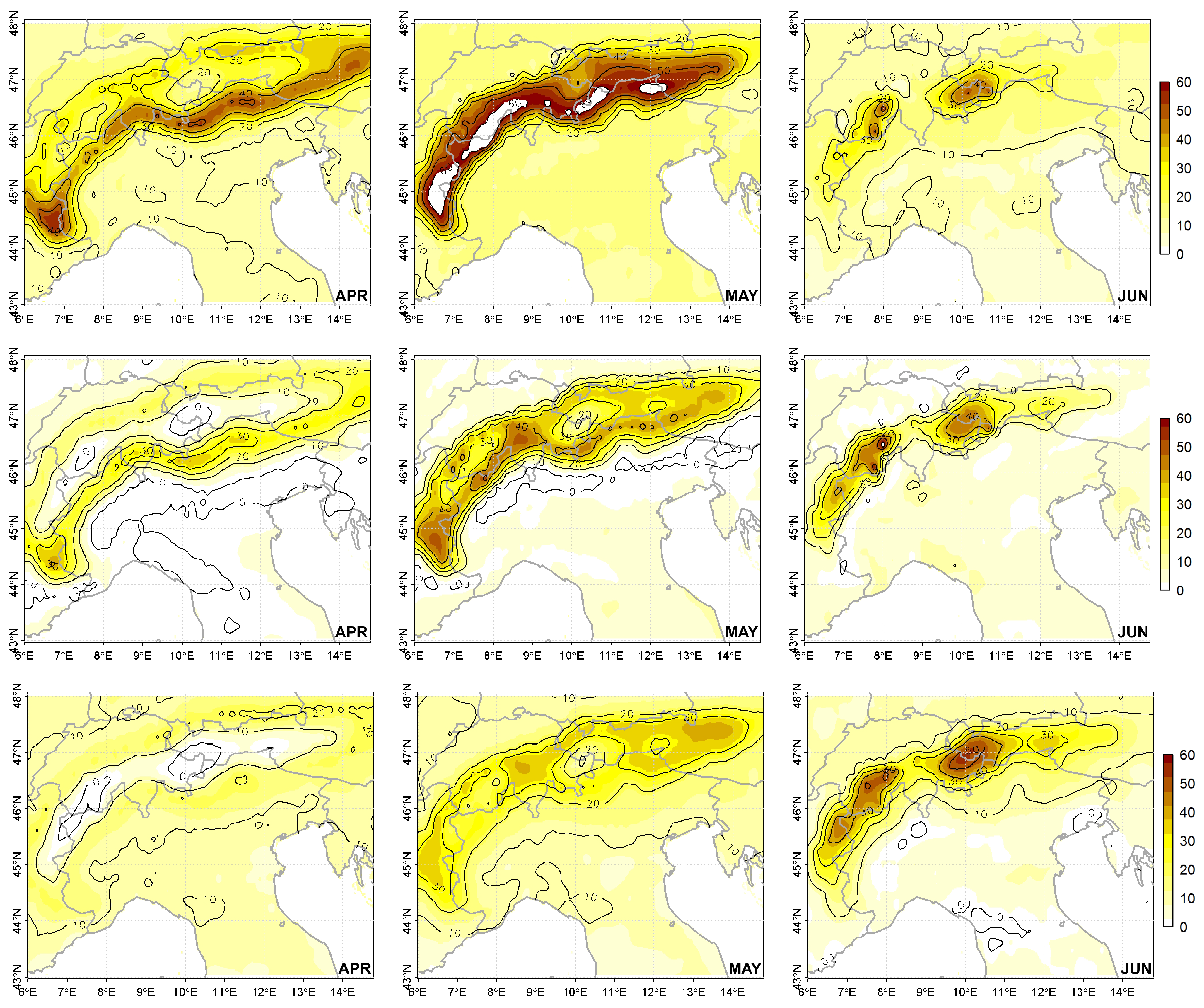
All these projections are obviously associated with temporal variation in the surface energy budget components. Figure 7 displays the differences in the various energy components ($\Delta$NR, $\Delta$SHF and $\Delta$LHF) between FC${}_{A2}$ and RC. It is apparent that $\Delta$NRs directly correspond to the snow cover differences (cf. upper panels of Figure 6). A change in the snow cover fraction causes a relevant difference in the surface albedo and consequently, a remarkable difference in the amount of incoming solar radiation and turbulent heat fluxes, thus affecting the amount of NR. It is also evident as $\Delta$NR tends to decrease in June when almost all of the territory is snowless in FCA2, while some snow patches still remain over the Alps in the RC. In fact, in the same regions where $\Delta$NRs are large, the turbulent heat flux anomalies (i.e., $\Delta$SHF and $\Delta$LHF) are remarkable. The characteristic distribution of $\Delta$SHF is directly linked to that of $\Delta$ST (cf. Figure 5) and of $\Delta$NR; $\Delta$SHF is remarkable only where $\Delta$NRs are large, and is negligible when $\Delta$NRs are lower than 10–20 W m${}^{-2}$. The pattern of $\Delta$LHF is similar to that of $\Delta$SHF, but shows a broader and weaker positive increments over the off-alpine areas (Figure 7c). This can be attributed to the properties of LHF that are associated with several factors such as air temperature, humidity, wind, vegetation, soil moisture as well as ST. In fact, $\Delta$LHF is represented by the transport of soil water into the atmosphere through ET. The positive increment of NR is mainly used to warm the soil surface and eventually, to warm the overlaying atmosphere in the boundary layer, rather than to increase ET significantly.

4.3. Number of Warm and Cold Days in the Future Climate

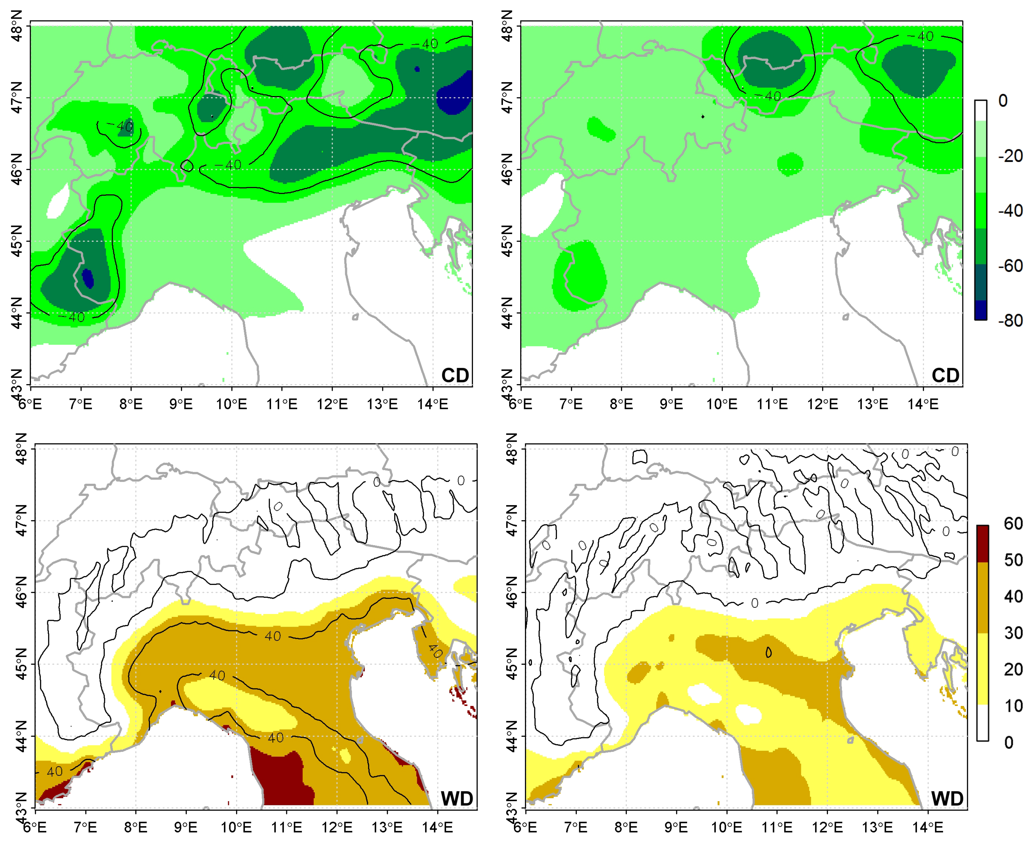
Figure 8 shows the annual number of cold and warm days, expressed as the average number of anomalies between FC${}_{A2}$ and RC and between FC${}_{B2}$ and RC. Again FC${}_{B2}$ shows a smaller number of cold/warm days than, but similar distribution with, FC${}_{A2}$. For the cold days (CDs), the anomaly is generally negative in the Alpine areas, implying a decrease in the number of CDs in FCs. This feature is particularly evident on the mountainous grid points and is more prominent over the Northern sides. Actually, in the RC, the grid points with more than 150 CDs occupy a large fraction of the Alps, while in FCs, these appear only in some limited areas around mountain peaks (not shown). In the plain areas, CDs almost disappear in FCs—the absolute number of the CD anomaly between FC${}_{A2}$ and RC is mostly lower than 20. This tendency is quite affirmative because the interannual variability in the number of CDs decreases (not shown). As a result, some small areas in which the number of CDs in FC${}_{A2}$ decrease by 80 or more are present in the extreme Southwestern Alps between France and Italy and in Slovenia, whereas the off-alpine areas in Northeastern Italy show deficits of about 60 days. In FC${}_{B2}$, similar features appear but with smaller values (deficit of 30 in Slovenia and 20 in the Southwestern Alps. For the warm days (WDs), positive increments are prevalent over the plain Po Valley areas, as expected; hence, there is an increase in the number of WDs in FCs. In some zones (e.g., the coastal region of Tuscany), the anomaly exceeds 40 days, which implies that the average summer in FC${}_{A2}$ will be hotter than the summer of 2003 that had an unprecedentedly strong heat wave in Europe [60]. Furthermore, the anomaly in the interannual variability of the number of WD doubles (not shown)—indicating the possibility of very long and intense heat waves that would exert wide negative impacts on the environment, human health, and agricultural production. In FC${}_{B2}$, areas of about 40 increment in WDs are present over the plain Po Valley, the coastal region of Tuscany, and some spots in the Piemonte region.

5. Conclusions

This study investigated the variations in the energy budget and soil temperature under future climate conditions over the Alps and Northern Italy. For this purpose, we employed a land surface model, called the University of TOrino model of land Processes Interaction with Atmosphere (UTOPIA). We also used the Regional Climate Model version 3 (RegCM3) to produce meteorological variables in future climates (FCs) based on the SRES A2 and B2 scenarios. UTOPIA was run over each grid point of the RegCM3 computational domain, with the boundary conditions provided by a subset of output data from RegCM3. This study also demonstrated the first-time application of UTOPIA to process a long time series of climatic data, over a wide domain and under varied meteorological regimes.

We discussed the variations in yearly energy budget components from the reference climate (RC) to FCs focusing on two sets of grid points—those below 500 m a.s.l. (considered plains) and those higher than 2000 m a.s.l. (considered high-mountain areas)—in order to quantify the importance of energy budget component variations in terms of geographical feature and topography influence. The most evident results in FCs include the following: (i) The increase in latent heat flux (and hence, evapotranspiration) during summertime over the plain areas as a direct consequence of the corresponding increment of net radiation; and (ii) the precedence of the snow-melting season of about one month over the mountainous areas, especially on the Italian side. As a result, the soil surface temperatures increase earlier during springtime over the mountainous areas with consequences that alter all components of the energy budget.

We also performed an analysis on the number of warm (above 30 ${}^{\circ }$C) and cold (below 0 ${}^{\circ }$C) days in FCs, based on the soil surface temperature. The number of warm days increases in the plain areas by 30 days or more with a larger interannual variability, while the number of cold days decreases significantly in the high-mountain areas; cold days almost disappear in the plains.

Overall, our results indicate some challenging behaviors of the energy budget components and soil temperature—in particular, the shortened snow-cover periods over the high-mountain areas and the increased number of warm days. Both will subsequently affect the regional radiative properties and water cycles and eventually have influences on human life and infrastructures, which are further discussed in [4]. Furthermore, this study demonstrates the applicability of the CLIPS method for the analysis of climate data as in reference [30] using the UTOPIA results obtained through the offline run that takes the meteorological variables from RegCM3 only as inputs. This choice was made by considering the well-known problem of the forcing-restore method used in the RegCM3 soil scheme (i.e., BATS) in representing soil water transfer parameterization which consequently affects soil temperature. Thus, this kind of the CLIPS method application opens the way for further analyses that could be performed using the current and/or other datasets.

References

- Chen, F.; Dudhia, J. Coupling an advanced land surface-hydrology model with the Penn State-NCAR MM5 modeling system. Part I: Model implementation and sensitivity. Mon. Weather Rev. 2001, 129, 569–585. [Google Scholar] [CrossRef]
- Levis, S. Modeling vegetation and land use in models of the Earth System. Wiley Interdiscip. Rev. Clim. Chang. 2010, 1, 840–856. [Google Scholar] [CrossRef]
- Pitman, A.J. The evolution of, and revolution in, land surface schemes designed for climate models. Int. J. Climatol. 2003, 23, 479–510. [Google Scholar] [CrossRef] [Green Version]
- Cassardo, C.; Park, S.K.; Galli, M.; Sungmin, O. Climate change over the high-mountain versus plain areas: Effects on the land surface hydrologic budget in the Alpine area and northern Italy. Hydrol. Earth Syst. Sci. 2018, 22, 3331–3350. [Google Scholar] [CrossRef]
- Robock, A.; Vinnikov, K.Y.; Srinivasan, G.; Entin, J.K.; Hollinger, S.E.; Speranskaya, N.A.; Liu, S.; Namkhai, A. The global soil moisture data bank. Bull. Amer. Meteorol. Soc. 2000, 81, 1281–1299. [Google Scholar] [CrossRef]
- Fan, Y.; van den Dool, H. Climate Prediction Center global monthly soil moisture data set at 0.5∘ resolution for 1948 to present. J. Geophys. Res. 2004, 109, D10102. [Google Scholar] [CrossRef]
- Reichle, R.H.; Koster, R.D.; Dong, J.; Berg, A.A. Global soil moisture from satellite observations, land surface models, and ground data: Implications for data assimilation. J. Hydrometeorol. 2004, 5, 430–442. [Google Scholar] [CrossRef]
- Wagner, W.; Naeimi, V.; Scipal, K.; de Jeu, R.; Martınez-Fernandez, J. Soil moisture from operational meteorological satellites. Hydrogeol. J. 2007, 15, 121–131. [Google Scholar] [CrossRef]
- Owe, M.; de Jeu, R.; Holmes, T. Multisensor historical climatology of satellite-derived global land surface moisture. J. Geophys. Res. 2008, 113, F01002. [Google Scholar] [CrossRef]
- Dorigo, W.A.; Wagner, W.; Hohensinn, R.; Hahn, S.; Paulik, C.; Xaver, A.; Gruber, A.; Drusch, M.; Mecklenburg, S.; van Oevelen, P.; et al. The international soil moisture network: A data hosting facility for global in situ soil moisture measurements. Hydrol. Earth Syst. Sci. 2011, 15, 1675–1698. [Google Scholar] [CrossRef]
- Petropoulos, G.P.; Ireland, G.; Barrett, B. Surface soil moisture retrievals from remote sensing: Current status, products and future trends. Phys. Chem. Earth Parts A/B/C 2015, 83–84, 36–56. [Google Scholar] [CrossRef]
- Seyfried, M.S.; Flerchinger, G.N.; Murdock, M.D.; Hanson, C.L.; van Vactor, S. Long-term soil temperature database, Reynolds Creek Experimental Watershed, Idaho, United States. Water Resour. Res. 2001, 37, 2843–2846. [Google Scholar] [CrossRef]
- Seyfried, M.; Link, T.; Marks, D.; Murdock, M. Soil temperature variability in complex terrain measured using fiber-optic distributed temperature sensing. Vadose Zone J. 2016, 15. [Google Scholar] [CrossRef]
- Hu, Q.; Feng, S. A daily soil temperature dataset and soil temperature climatology of the contiguous United States. J. Appl. Meteorol. Climatol. 2003, 42, 1139–1156. [Google Scholar] [CrossRef]
- Sobrino, J.A.; Romaguera, M. Land surface temperature retrieval from MSG1-SEVIRI data. Remote Sens. Environ. 2004, 92, 247–254. [Google Scholar] [CrossRef]
- Li, Z.-L.; Tang, B.-H.; Wu, H.; Ren, H.; Yan, G.; Wan, Z.; Trigo, I.F.; Sobrino, J.A. Satellite-derived land surface temperature: Current status and perspectives. Remote Sens. Environ. 2013, 131, 14–37. [Google Scholar] [CrossRef] [Green Version]
- Wan, Z. New refinements and validation of the Collection-6 MODIS land-surface temperature/emissivity products. Remote Sens. Environ. 2014, 140, 36–45. [Google Scholar] [CrossRef]
- Cassardo, C.; Ruti, P.M.; Cacciamani, C.; Longhetto, A.; Paccagnella, T.; Bargagli, A. CLIPS experiment. First step: Model intercomparison and validation against experimental data. MAP Newslett. 1997, 7, 74–75. [Google Scholar]
- Shao, Y.; Henderson-Sellers, A. Validation of soil moisture simulation in land surface parameterisation schemes with HAPEX data. Glob. Planet. Chang. 1996, 13, 11–46. [Google Scholar] [CrossRef]
- Ruti, P.M.; Cassardo, C.; Cacciamani, C.; Paccagnella, T.; Longhetto, A.; Bargagli, A. Intercomparison between BATS and LSPM surface schemes, using point micrometeorological data set. Contrib. Atmos. Phys. 1997, 70, 201–220. [Google Scholar]
- Cassardo, C.; Balsamo, G.P.; Pelosini, R.; Cacciamani, C.; Cesari, D.; Paccagnella, T.; Longhetto, A. Initialization of soil parameters in LAM: CLIPS experiment. MAP Newslett. 1999, 11, 26–27. [Google Scholar]
- Cassardo, C.; Balsamo, G.P.; Cacciamani, C.; Cesari, D.; Paccagnella, T.; Pelosini, R. Impact of soil surface moisture initialization on rainfall in a limited area model: A case study of the 1995 South Ticino flash flood. Hydrol. Process. 2002, 16, 1301–1317. [Google Scholar] [CrossRef]
- Cassardo, C.; Park, S.K.; Thakuri, B.M.; Priolo, D.; Zhang, Y. Soil surface energy and water budgets during a monsoon season in Korea. J. Hydrometeorol. 2009, 10, 1379–1396. [Google Scholar] [CrossRef]
- Zhu, J.; Liang, X.-Z. Regional climate model simulation of U.S. soil temperature and moisture during 1982–2002. J. Geophys. Res. 2005, 110, D24110. [Google Scholar] [CrossRef]
- Tsiros, I.X.; Dimopoulos, I.F. An evaluation of the performance of the soil temperature simulation algorithms used in the PRZM model. J. Environ. Sci. Health Part A 2007, 42, 661–670. [Google Scholar] [CrossRef] [PubMed]
- Sándor, R.; Fodor, N. Simulation of soil temperature dynamics with models using different concepts. Sci. World J. 2012. [Google Scholar] [CrossRef] [PubMed]
- Sándor, R.; Barcza, Z.; Acutis, M.; Doro, L.; Hidy, D.; Köchy, M.; Minet, J.; Lellei-Kovács, E.; Ma, S.; Perego, A.; et al. Multi-model simulation of soil temperature, soil water content and biomass in Euro-Mediterranean grasslands: Uncertainties and ensemble performance. Eur. J. Agron. 2017, 88, 22–40. [Google Scholar] [CrossRef] [Green Version]
- Bhattacharya, A.; Mandal, M. Evaluation of Noah land-surface models in predicting soil temperature and moisture at two tropical sites in India. Meteorol. Appl. 2015, 22, 505–512. [Google Scholar] [CrossRef]
- Hu, G.; Zhao, L.; Wu, X.; Li, R.; Wu, T.; Xie, C.; Qiao, Y.; Shi, J.; Cheng, G. An analytical model for estimating soil temperature profiles on the Qinghai-Tibet Plateau of China. J. Arid Land 2016, 8, 232–240. [Google Scholar] [CrossRef]
- Park, S.K.; O, S.; Cassardo, C. Soil temperature response in Korea to a changing climate using a land surface model. Asia-Pac. J. Atmos. Sci. 2017, 53, 457–470. [Google Scholar] [CrossRef]
- Hong, S.; Yu, X.; Park, S.K.; Choi, Y.-S.; Myoung, B. Assessing optimal set of implemented physical parameterization schemes in a multi-physics land surface model using genetic algorithm. Geosci. Model Dev. 2014, 7, 2517–2529. [Google Scholar] [CrossRef] [Green Version]
- Hong, S.; Park, S.K.; Yu, X. Scheme-based optimization of land surface model using a micro-genetic algorithm: Assessment of its performance and usability for regional applications. Sci. Online Lett. Atmos. 2015, 11, 129–133. [Google Scholar] [CrossRef]
- Park, S.; Park, S.K. Parameterization of the snow-covered surface albedo in the Noah-MP Version 1.0 by implementing vegetation effects. Geosci. Model Dev. 2016, 9, 1073–1085. [Google Scholar] [CrossRef] [Green Version]
- Gim, H.-J.; Park, S.K.; Kang, M.; Thakuri, B.M.; Kim, J.; Ho, C.-H. An improved parameterization of the allocation of assimilated carbon to plant parts in vegetation dynamics for Noah-MP. J. Adv. Model. Earth Syst. 2017, 9, 1776–1794. [Google Scholar] [CrossRef] [Green Version]
- Im, E.-S.; Coppola, E.; Giorgi, F.; Bi, X. Local effects of climate change over the Alpine region: A study with a high resolution regional climate model with a surrogate climate change scenario. Geophys. Res. Lett. 2010, 37, L05704. [Google Scholar] [CrossRef]
- Torma, C.; Coppola, E.; Giorgi, F.; Bartholy, J.; Pongrácz, R. Validation of a high-resolution version of the regional climate model RegCM3 over the Carpathian basin. J. Hydrometeorol. 2011, 12, 84–100. [Google Scholar] [CrossRef]
- Coppola, E.; Verdecchia, M.; Giorgi, F.; Colaiuda, V.; Tomassetti, B.; Lombardi, A. Changing hydrological conditions in the Po basin under global warming. Sci. Total Environ. 2014, 493, 1183–1196. [Google Scholar] [CrossRef] [PubMed]
- Faggian, P. Climate change projections for Mediterranean region with focus over Alpine region and Italy. J. Environ. Sci. Eng. B 2015, 4, 482–500. [Google Scholar]
- Alo, C.A.; Anagnostou, E.N. A sensitivity study of the impact of dynamic vegetation on simulated future climate change over Southern Europe and the Mediterranean. Int. J. Climatol. 2017, 37, 2037–2050. [Google Scholar] [CrossRef]
- Elguindi, N.; Bi, X.; Giorgi, F.; Nagarajan, B.; Pal, J.; Solmon, F.; Rauscher, S.; Zakey, A. RegCM Version 3.1 User’s Guide; Technical Report; International Centre for Theoretical Physics: Trieste, Italy, 2007; p. 57. [Google Scholar]
- Cassardo, C. The University of TOrino Model of Land Process Interaction with Atmosphere (UTOPIA) Version 2015; Tech. Rep.; CCCPR/SSRC-TR-2015-1, CCCPR/SSRC; Ewha Womans University: Seoul, Korea, 2015; p. 184. [Google Scholar]
- Gao, X.J.; Pal, J.S.; Giorgi, F. Projected changes in mean and extreme precipitation over the Mediterranean region from a high resolution double nested RCM simulation. Geophys. Res. Lett. 2006, 33, L03706. [Google Scholar] [CrossRef]
- Smiatek, G.; Kunstmann, H.; Knoche, R.; Marx, A. Precipitation and temperature statistics in high-resolution regional climate models: Evaluation for the European Alps. J. Geophys. Res. 2009, 114, D19107. [Google Scholar] [CrossRef]
- Ballester, J.; Rodó, X.; Giorgi, F. Future changes in Central Europe heat waves expected to mostly follow summer mean warming. Clim. Dyn. 2010, 35, 1191–1205. [Google Scholar] [CrossRef]
- Coppola, E.; Giorgi, F. An assessment of temperature and precipitation change projections over Italy from recent global and regional climate model simulations. Int. J. Climatol. 2010, 30, 11–32. [Google Scholar] [CrossRef]
- Rauscher, S.A.; Coppola, E.; Piani, C.; Giorgi, F. Resolution effects on regional climate model simulations of seasonal precipitation over Europe. Clim. Dyn. 2010, 35, 685–711. [Google Scholar] [CrossRef]
- Heinrich, G.; Gobiet, A.; Mendlik, T. Extended regional climate model projections for Europe until the mid-twenty first century: Combining ENSEMBLES and CMIP3. Clim. Dyn. 2014, 42, 521–535. [Google Scholar] [CrossRef]
- Nadeem, I.; Formayer, H. Sensitivity studies of high-resolution RegCM3 simulations of precipitation over the European Alps: The effect of lateral boundary conditions and domain size. Theor. Appl. Climatol. 2016, 126, 617–630. [Google Scholar] [CrossRef]
- Alexandri, G.; Georgoulias, A.K.; Zanis, P.; Katragkou, E.; Tsikerdekis, A.; Kourtidis, K.; Meleti, C. On the ability of RegCM4 regional climate model to simulate surface solar radiation patterns over Europe: An assessment using satellite-based observations. Atmos. Chem. Phys. 2015, 15, 13195–13216. [Google Scholar] [CrossRef]
- Chiacchio, M.; Solmon, F.; Giorgi, F.; Stackhouse, P.; Wild, M. Evaluation of the radiation budget with a regional climate model over Europe and inspection of dimming and brightening. J. Geophys. Res. 2015, 120, 1951–1971. [Google Scholar] [CrossRef] [Green Version]
- Giorgi, F.; Anyah, R.O. The road towards RegCM4. Clim. Res. 2012, 52, 3–6. [Google Scholar] [CrossRef]
- Rajalakshmi, D.; Jagannathan, R.; Geethalakshmi, V. Comparative performance of RegCM model versions in simulating climate change projection over Cauvery Delta zone. Indian J. Sci. Technol. 2013, 6, 5115–5119. [Google Scholar]
- Cassardo, C.; Ji, J.J.; Longhetto, A. A study of the performances of a Land Surface Process Model (LSPM). Bound.-Layer Meteorol. 1995, 72, 87–121. [Google Scholar] [CrossRef]
- Cassardo, C.; Carena, E.; Longhetto, A. Validation and sensitivity tests on improved parametrizations of a land surface process model (LSPM) in the Po Valley. Il Nuovo Cimento 1998, 21, 189–213. [Google Scholar]
- Carlson, T.N.; Boland, F.E. Analysis of urban-rural canopy using a surface heat flux/temperature model. J. Appl. Meteorol. 1978, 17, 998–1013. [Google Scholar] [CrossRef]
- Arora, V.K. Modeling vegetation as a dynamic component in soil-vegetation-atmosphere transfer schemes and hydrological models. Rev. Geophys. 2002, 40, 1–26. [Google Scholar] [CrossRef]
- Petropoulos, G.; Carlson, T.N.; Wooster, M.J. An overview of the use of the SimSphere soil vegetation atmosphere transfer (SVAT) model for the study of land-atmosphere interactions. Sensors 2009, 9, 4286–4308. [Google Scholar] [CrossRef] [PubMed] [Green Version]
- Cassardo, C.; Loglisci, N.; Gandini, D.; Qian, M.W.; Niu, Y.P.; Ramieri, P.; Pelosini, R.; Longhetto, A. The flood of November 1994 in Piedmont, Italy: A quantitative simulation. Hydrol. Process. 2002, 16, 1275–1299. [Google Scholar] [CrossRef]
- Cassardo, C.; Loglisci, N.; Paesano, G.; Rabuffetti, D.; Qian, M.W. The hydrological balance of the October 2000 flood in Piedmont, Italy: Quantitative analysis and simulation. Phys. Geogr. 2006, 27, 411–434. [Google Scholar] [CrossRef]
- Cassardo, C.; Mercalli, L.; Cat Berro, D. Characteristics of the summer 2003 heat wave in Piedmont, Italy, and its effects on water resources. J. Korean Meteorol. Soc. 2007, 43, 195–221. [Google Scholar]
- Galli, M.; Oh, S.; Cassardo, C.; Park, S.K. The occurrence of cold spells in the Alps related to climate change. Water 2010, 2, 363–380. [Google Scholar] [CrossRef]
- Francone, C.; Cassardo, C.; Richiardone, R.; Confalonieri, R. Sensitivity analysis and investigation of the behaviour of the UTOPIA land-surface process model: A case study for vineyards in northern Italy. Bound.-Layer Meteorol. 2012, 144, 419–430. [Google Scholar] [CrossRef]
- Feng, J.; Liu, X.; Cassardo, C.; Longhetto, A. A model of plant transpiration and stomatal regulation under the condition of water stress. J. Desert Res. 1997, 17, 59–66. [Google Scholar]
- Loglisci, N.; Qian, M.W.; Cassardo, C.; Longhetto, A.; Giraud, C. Energy and water balance at soil-air interface in a Sahelian region. Adv. Atmos. Sci. 2001, 18, 897–909. [Google Scholar]
- Qian, Y.; Giorgi, F.; Huang, Y.; Chameides, W.L.; Luo, C. Simulation of anthropogenic sulfur over East Asia with a regional coupled chemistry-climate model. Tellus B 2001, 53, 171–191. [Google Scholar] [CrossRef]
- Zhang, Y.; Cassardo, C.; Ye, C.; Galli, M.; Vela, N. The role of the land surface processes in the rainfall generated by a landfall typhoon: A simulation of the Typhoon Sepat (2007). Asia-Pac. J. Atmos. Sci. 2011, 47, 63–77. [Google Scholar] [CrossRef]
- Déqué, M.; Somot, S. Analysis of heavy precipitation for France using high resolution ALADIN RCM simulations. Idöjárás 2008, 112, 179–190. [Google Scholar]
- Tramblay, Y.; Ruelland, D.; Somot, S.; Bouaicha, R.; Servat, E. High-resolution Med-CORDEX regional climate model simulations for hydrological impact studies: A first evaluation of the ALADIN-Climate model in Morocco. Hydrol. Earth Syst. Sci. 2013, 17, 3721–3739. [Google Scholar] [CrossRef]
- Wang, C.; Jones, R.; Perry, M.; Johnson, C.; Clark, P. Using an ultrahigh-resolution regional climate model to predict local climatology. Q. J. R. Meteorol. Soc. 2013, 139, 1964–1976. [Google Scholar] [CrossRef] [Green Version]
- Cantet, P.; Déqué, M.; Palany, P.; Maridet, J.-L. The importance of using a high-resolution model to study the climate change on small islands: the Lesser Antilles case. Tellus A 2014, 66, 24065. [Google Scholar] [CrossRef]
- Rummukainen, M. Added value in regional climate modeling. WIREs Clim. Chang. 2016, 7, 145–159. [Google Scholar] [CrossRef]
- Dickinson, R.E.; Henderson-Sellers, A.; Kennedy, P.J. Biosphere-Atmosphere Transfer Scheme (BATS) Version 1e as Coupled to the NCAR Community Climate Model; NCAR Technical Note; NCAR/TN-387+STR; NCAR: Boulder, CO, USA, 1993. [Google Scholar] [CrossRef]
- Masson, V.; Champeaux, J.L.; Chauvin, F.; Meriguet, C.; Lacaze, R. A global database of land surface parameters at 1 km resolution in meteorological and climate models. J. Clim. 2003, 16, 1261–1282. [Google Scholar] [CrossRef]
- Champeaux, J.L.; Masson, V.; Chauvin, F. ECOCLIMAP: A global database of land surface parameters at 1 km resolution. Meteorol. Appl. 2005, 12, 29–32. [Google Scholar] [CrossRef]
- Paulsen, J.; Körner, C. GIS-analysis of tree-line elevation in the Swiss Alps suggests no exposure effect. J. Veg. Sci. 2001, 12, 817–824. [Google Scholar] [CrossRef]
- Gehrig-Fasel, J.; Guisan, A.; Zimmermann, N.E. Tree line shifts in the Swiss Alps: Climate change or land abandonment? J. Veg. Sci. 2007, 18, 571–582. [Google Scholar] [CrossRef]
- Heinimann, H.R. A concept in adaptive ecosystem management—An engineering perspective. For. Ecol. Manag. 2009, 259, 848–856. [Google Scholar] [CrossRef]
- Nakićenović, N.; Alcamo, J.; Davis, G.; de Vries, B.; Fenhann, J.; Gaffin, S.; Gregory, K.; Grübler, A.; Jung, T.Y.; Kram, T.; et al. Special Report on Emissions Scenarios: A Special Report of Working Group III of the Intergovernmental Panel on Climate Change; Cambridge University Press: Cambridge, UK, 2000; p. 599. [Google Scholar]
- Brovkin, V.; Boysen, L.; Arora, V.K.; Boisier, J.P.; Cadule, P.; Chini, L.; Claussen, M.; Friedlingstein, P.; Gayler, V.; van den Hurk, B.J.J.M.; et al. Effect of anthropogenic land-use and land-cover changes on climate and land carbon storage in CMIP5 projections for the twenty-first century. J. Clim. 2013, 26, 6859–6881. [Google Scholar] [CrossRef]
- Hallgren, W.; Schlosser, C.A.; Monier, E.; Kicklighter, D.; Sokolov, A.; Melillo, J. Climate impacts of a large-scale biofuels expansion. Geophys. Res. Lett. 2013, 40, 1624–1630. [Google Scholar] [CrossRef] [Green Version]
- Kicklighter, D.W.; Cai, Y.; Zhuang, Q.; Parfenova, E.I.; Paltsev, S.; Sokolov, A.P.; Melillo, J.M.; Reilly, J.M.; Tchebakova, N.M.; Lu, X. Potential influence of climate-induced vegetation shifts on future land use and associated land carbon fluxes in Northern Eurasia. Environ. Res. Lett. 2014, 9, 035004. [Google Scholar] [CrossRef] [Green Version]
- Krüger, L.F.; da Rocha, R.P.; Reboita, M.S.; Ambrizzi, T. RegCM3 nested in HadAM3 scenarios A2 and B2: projected changes in extratropical cyclogenesis, temperature and precipitation over the South Atlantic Ocean. Clim. Chang 2012, 113, 599–621. [Google Scholar] [CrossRef]
- Zanis, P.; Ntogras, C.; Zakey, A.; Pytharoulis, I.; Karacostas, T. Regional climate feedback of anthropogenic aerosols over Europe using RegCM3. Clim. Res. 2012, 52, 267–278. [Google Scholar] [CrossRef] [Green Version]
- Jamieson, P.D.; Brooking, I.R.; Porter, J.R.; Wilson, D.R. Prediction of leaf appearance in wheat: A question of temperature. Field Crops Res. 1995, 41, 35–44. [Google Scholar] [CrossRef]
- Bollero, G.A.; Bullock, D.G.; Hollinger, S.E. Soil temperature and planting date effects on corn yield, leaf area, and plant development. Agron. J. 1996, 88, 385–390. [Google Scholar] [CrossRef]
- Nishar, A.; Bader, M.K.-F.; O’Gorman, E.J.; Deng, J.; Breen, B.; Leuzinger, S. Temperature effects on biomass and regeneration of vegetation in a geothermal area. Front. Plant. Sci. 2017, 8, 249. [Google Scholar] [CrossRef] [PubMed]
- Jones, H.G.; Hillis, R.M.; Gordon, S.L.; Brennan, R.M. An approach to the determination of winter chill requirements for different Ribes cultivars. Plant Biol. 2012, 15 (Suppl. 1), 18–27. [Google Scholar] [CrossRef] [PubMed]
- Hatfield, J.L.; Pruege, J.H. Temperature extremes: Effect on plant growth and development. Weather Clim. Extremes 2015, 10, 4–10. [Google Scholar] [CrossRef]
- Zavaleta, E.S.; Thomas, B.D.; Chiariello, N.R.; Asner, G.P.; Shaw, M.R.; Field, C.B. Plants reverse warming effect on ecosystem water balance. Proc. Natl. Acad. Sci. USA 2003, 100, 9892–9893. [Google Scholar] [CrossRef] [PubMed] [Green Version]
- Coppola, E.; Raffaele, F.; Giorgi, F. Impact of climate change on snow melt driven runoff timing over the Alpine region. Clim. Dyn. 2016. [Google Scholar] [CrossRef]
Figure 1.
Geographic map (left; from Google Maps) in which the black box indicates a computational domain (right) with a total of 720 grid points for the UTOPIA model run. The elevation (h) of blue grid points is 500 m a.s.l. (plain area), whereas that of red grid points is 2000 m a.s.l. (high-mountain area). The grey grid points represent normal mountains with an elevation between 500 and 2000 m a.s.l.
Figure 2.
Annual cycles of the 10-day average values of the surface energy budget components for plains (i.e., grid points located below 500 m a.s.l.) for (a) RC (with standard deviations; vertical bars), (b) FC – RC, and (c) FC – RC. Here, NR is the net radiation, SHF is the sensible heat flux, LHF is the latent heat flux, and CHF is the conductive heat flux. The units are W m.
Figure 3.
Same as in Figure 2 but for the high mountains (i.e., grid points located above 2000 m a.s.l.). Grey bars in the lower portion in (a) represent the snow cover (in m) in the RC varying from 0 to 1 m; in (b,c), the snow cover difference (SN; in m) between the corresponding FC and RC varies from −0.5 to 0.5 m. The periods of snow ablation (late spring) and accumulation (mid or late autumn) are well identified.
Figure 4.
Annual cycles of the 10-day average soil temperatures (in C) in the upper soil layer (5 cm deep) in the RC (black), FC (red) and FC (green) at (a) plains and (b) high mountains. The standard deviations are also plotted (vertical bars).
Figure 5.
Soil temperature differences (in C) in the surface soil layer between FC and the RC (upper panels) and between FC and the RC (lower panels) for April, May, and June.
Figure 6.
Differences between FC and the RC in snow cover (in %; upper panels) and in snow depth (in m; lower panels) for April, May, and June.
Figure 7.
Differences between FC and the RC in net radiation (NR; top panels), sensible heat flux (SHF; middle panels), and latent heat flux (LHF, i.e., evapotranspiration; bottom panels) for April, May, and June. Units are W m.
Figure 8.
Number of days, expressed as anomalies between FC and the RC (left panels) and between FC and the RC (right panels), for cold days (CDs; TC) and warm days (WDs; TC). T is the daily mean temperature of the soil surface layer.
© 2018 by the authors. Licensee MDPI, Basel, Switzerland. This article is an open access article distributed under the terms and conditions of the Creative Commons Attribution (CC BY) license (http://creativecommons.org/licenses/by/4.0/).
Share and Cite
MDPI and ACS Style
Cassardo, C.; Park, S.K.; O, S.; Galli, M. Projected Changes in Soil Temperature and Surface Energy Budget Components over the Alps and Northern Italy. Water 2018, 10, 954. https://doi.org/10.3390/w10070954
AMA Style
Cassardo C, Park SK, O S, Galli M. Projected Changes in Soil Temperature and Surface Energy Budget Components over the Alps and Northern Italy. Water. 2018; 10(7):954. https://doi.org/10.3390/w10070954
Chicago/Turabian StyleCassardo, Claudio, Seon Ki Park, Sungmin O, and Marco Galli. 2018. "Projected Changes in Soil Temperature and Surface Energy Budget Components over the Alps and Northern Italy" Water 10, no. 7: 954. https://doi.org/10.3390/w10070954
Note that from the first issue of 2016, this journal uses article numbers instead of page numbers. See further details here.