Model-Based Analysis of Macrophytes Role in the Flow Distribution in the Anastomosing River System


1
Department of Hydraulic Engineering, Faculty of Civil and Environmental Engineering, Warsaw University of Life Sciences—SGGW, 02-787 Warsaw, Poland
2
Faculty of Building Services, Hydro and Environmental Engineering, Warsaw University of Technology, 00-661 Warsaw, Poland
*
Author to whom correspondence should be addressed.
Water 2018, 10(7), 953; https://doi.org/10.3390/w10070953
Submission received: 4 June 2018
/
Revised: 3 July 2018
/
Accepted: 13 July 2018
/
Published: 18 July 2018
(This article belongs to the Special Issue Riparian Vegetation in River Functioning)
Abstract
:The impact of vegetation on the hydrology and geomorphology of aquatic ecosystems has been studied intensively in recent years. Numerous hydraulic models developed to date help to understand and quantitatively assess the influence of in-stream macrophytes on a channel’s hydraulic conditions. However, special focus is placed on single-thread rivers, leaving anastomosing rivers practically uninvestigated. To fill this gap, the objective of this study was to investigate the impact of vegetation on flow distribution in a complex anastomosing river system situated in northeastern Poland. The newly designed, one-dimensional, steady-flow model, dedicated for anastomosing rivers used in this study indicated high influence of vegetation on water flow distribution during the whole year in general, but—as expected—significantly higher in the summer season. Simulations of in-stream vegetation removal in selected channels reflected in Manning’s coefficient alterations caused relatively high discharge transitions during the growing season. This proved the significance of feedback between process of plants growth and distribution of flow in anabranches. The results are unique and relevant and could be successfully considered for the protection of semi-natural anabranching rivers.
1. Introduction
In recent years, there has been an increasing recognition of the role of vegetation in hydrology and fluvial geomorphology, supported by numerous studies documenting its influence on river channel morphological processes and geomorphic forms [1,2,3]. Riparian and aquatic vegetation, depending on their structure, density, coverage, etc. can affect river morphology in different ways, by altering the flow and subsequently the sediment balance through hydraulic resistance [4,5,6]. Numerous studies have described the empirical relationships between biological and physical characteristics in aquatic ecosystems [7,8]; nonetheless, more quantitative understanding, linking current knowledge with predictive models is required [9]. One of the examples of model-based assessment of vegetation impact on river pattern and morphodynamics was presented by Oorschot et al. [10]. In their study of a single-channel meandering river, they used a 2D sediment routing model coupled with a dynamic vegetation model. The study results indicated that models with dynamic vegetation, compared to static, give a different morphological response of a meandering channel. The first approach indicated meandering maintenance and the second one a reduction of morphodynamics over time and transformation of the river system into being vegetation-dominated. It stresses the fact that vegetation affects but also is affected by morphological processes.
The complexity of the biological and physical links escalates for multi-channel rivers characterized by intricate flow conditions and hydraulics. Most previous research has used numerical models in multichannel rivers that focused on braided rivers exploring flow–vegetation interactions [11,12,13] as well as sediment transport as a control on channel pattern [14,15]. A broad review evaluating the modeling frameworks appropriate for simulating the morphodynamics of braided rivers was given by Williams et al. [16]. The review covers a whole range of models varying from 1D to 3D and from reach to catchment scale. According to the authors, a 2D physics-based approach offers the highest potential for simulating braided river morphodynamics. In the study by Jowett and Duncan [17], a comparison of 1D and 2D model predictions of water depth and velocity is presented. The results indicate that the correlation between predicted and measured depths and velocities was higher for 1D than for 2D models, but 2D models gave more accurate predictions outside the calibration range of 1D models. Therefore, either 1D or 2D models are suitable for braided rivers modeling, and if done well, only small differences between the results should be obtained [17].
Anastomosing rivers constitute different type of multi-channel river systems. Their stable channels, which are separated by vegetated (floodplain) islands, occur in a variety of climatic conditions: subarctic, temperate, tropical and arid regions [18,19]. They are reported to form via avulsion, in which new channels (anabranches) form when water breaks through erosion-resistant banks and begins to incise gradually into the floodplain [20,21,22,23,24]. Numerous hypotheses explain avulsion triggering, which is indispensable for the creation and maintenance of anabranches. Among them the most widely applicable are a highly variable flood-prone flow regime [19,23] and localized flow vegetation obstacles [20,22]. The role of vegetation in influencing anastomosing river hydrology and geomorphology is complex, and—as stated by Tooth and Nanson [25]—needs to be assessed more fully, based on the data from a variety of rivers, before any generalizations can be made. The most comprehensive studies describing the impact of vegetation on anastomosing system formation concerned the River Okavango (Botswana) [20,22,26,27,28]. The authors, in their studies, created a conceptual model of the formation of the anastomosing system, which was assumed to be mainly controlled by the growth of bank and in-channel vegetation. Moreover, a theoretical description of the interaction of vegetation–channel geometry was provided. According to the authors, vegetation-induced flow velocity decrease and sediment aggradation initiates feedback mechanisms involving further invasion of aquatic plants in the channel, reducing flow rate and causing elevation of the channel water surface. This in turn increases the rate of water loss from the channel, accelerating blockage and aggradation. Similar mechanisms were described by Wende and Nanson [29], who examined the mechanisms of anabranch formation in Western Australia and emphasized the crucial role of vegetation.
However, besides qualitative, more quantitative, process-based studies recognizing the role of vegetation in influencing anabranching river hydrology and geomorphology are required. The hydraulic geometry of anabranching rivers remained unstudied until Tabata and Hickin [30] investigated a 10-km long reach of the upper Columbia River (Canada). They concluded in their study concerning the hydraulic efficiency of the anastomosing Columbia River that there is a great need for additional studies investigating inter-channel hydraulic properties and flow conditions in anastomosing rivers. Moreover, the little data available for anabranching rivers hints at formative processes not examined by hydraulic geometry and vegetation [31]. One of the examples of anastomosing river modeling was presented by Van et al. [32] who developed a 1D, steady-state HEC-RAS model for the anastomosing section of the Mekong river. However, they declared no field measurements on the flow distribution and river cross-sections, and limited their research only to one bifurcation without taking into account the detailed role of vegetation in flow distribution. Another attempt of anastomosing river modeling was made by Gibson and Pasternack [33], who developed a 1D and 2D model for three morphologically different reaches among which, anastomosing could be found. Although only one bifurcation was modeled, the authors found 1D model simulations underwhelming and split flow modeling to be an intermediate level of complexity. Therefore, and additional investigation improving split flow modeling is required.
Hydraulic modeling using 1D [34,35,36] and 2D [10,17,37] models is widely used to describe water flow in rivers. Modeling of hydraulic processes, flow and water-surface elevations in a fluvial system is influenced by vegetation contributing to roughness or overall flow resistance. Total roughness can be either partitioned to determine the relative contributions of vegetation type, distribution and morphology [38], or combined into a single parameter including the impact of vegetation density and morphology [39]. In hydraulic models, vegetation induced roughness is very often expressed in terms of the Manning’s coefficient through the Manning’s equation for uniform flow [40,41,42]. Although it was stated that Manning’s equation might be inappropriate in cases where the drag force is dominant over the bed friction [43], at the reach scale, the results are reliable [44,45]. Therefore, it is a widely accepted methodology in stream resistance evaluation, especially in vegetated areas [46] and was successfully incorporated in numerous studies investigating impact of vegetation on water flow, depth and velocity [47,48]. The importance of Manning’s coefficient assignment in the accuracy of hydraulic models was raised by Yang et al. [49] who found it highly difficult as roughness depends on flow circumstances, a stream’s geomorphology and physical conditions. To reduce the uncertainties to the greatest possible extent, field measurements can be conducted following Frias et al. [50], who recommended accurate and dense measurements of the river bed using GPS instead of incorporating Digital Elevation Models. The Manning’s coefficient is varied due to the changing discharge and diverse vegetational influence over the year [51,52,53]. There are numerous methods estimating flow resistance based on Manning’s coefficient that describe open-channel flow in a simplified but accurate way [54]. Most models focus on the calibration of the roughness parameter which, together with the geometry, is considered to have significant impact on flow modeling [55].
A model’s sensitivity analysis can be used to evaluate the magnitude of the dependency of model computations on certain modeling assumptions, e.g., parameter values. In other words, it is the study of how the different input variations of a model influence the variability of its output. It can be divided into two broad categories: local and global sensitivity analysis [56]. The local sensitivity is the sensitivity of the model output when the impact of small input parameter perturbations near its nominal values is considered. Global sensitivity determines the effect of the input parameters’ variation (due to parameter uncertainty) on model output [57,58]. In this study, focused on investigation of vegetation influence on water distribution in anastomosing river system, local sensitivity analysis is evaluated.
Studies on the modeling of multi-channel river systems mainly use 2D models, solving the momentum equation and mass conservation in distributing flow between side channels, which does not require detailed discharge measurements [11,12,13,17]. In cases where 1D models were used and the energy conservation equation was solved, the modeling was limited to only one bifurcation, as for proper model validation discharge measurements in all anabranches are required [32]. In experiments investigating vegetation–flow interactions and more complex geomorphological responses [10,11,12,13], upstream boundary conditions of flow were fixed either as a hydrograph or a constant flow. For single-channel rivers, it is appropriate and it is usually derived from discharge measurements. In multi-channel rivers, flow is distributed between side-channels and the distribution is highly related to flow obstacles in each channel and the channel geometry. A decrease of flow in one anabranch causes an increase in another and the effect propagates to downstream and upstream channels. This means that upstream boundary conditions of river flow in each anabranch remain unknown. Therefore, to be able to model complex interactions between biological and physical characteristics in anastomosing rivers, a reliable model, reflecting accurate flow distribution, is required. In other words, we cannot investigate complex feedbacks in an anastomosing system unless we take “one step back” and make sure that the flow rate in each anabranch is accurately simulated. 2D models are usually evaluated against water depths and velocities, but a remaining hindrance to wide acceptance of 2D modeling is the lack of standards for 2D-model evaluation [59]. Their structure is based on Digital Elevation Model (DEM) [40]. Light Detection and Ranging (LIDAR) derived DEMs are suitable for reflecting the geometry of a floodplain, but, since red laser does not penetrate through water table, it does not represent channel’s geometry accurately [60]. That the river reach investigated in this study consists of interconnected river channels with average width equal to 3 m convinced us that the use of 1D model supported by detailed field measurements of discharge distribution and channel’s geometry is the most suitable.
Against this background, the objective of this study was to investigate the impact of vegetation on flow distribution in a complex anastomosing river system situated in northeastern Poland. To this end, a newly designed 1D, steady-flow model, dedicated for anastomosing rivers was used. By means of mathematical simulations, model sensitivity analysis on vegetation changes was conducted to reflect its impact on flow distribution between anabranches.
2. Materials and Methods
2.1. Site Description
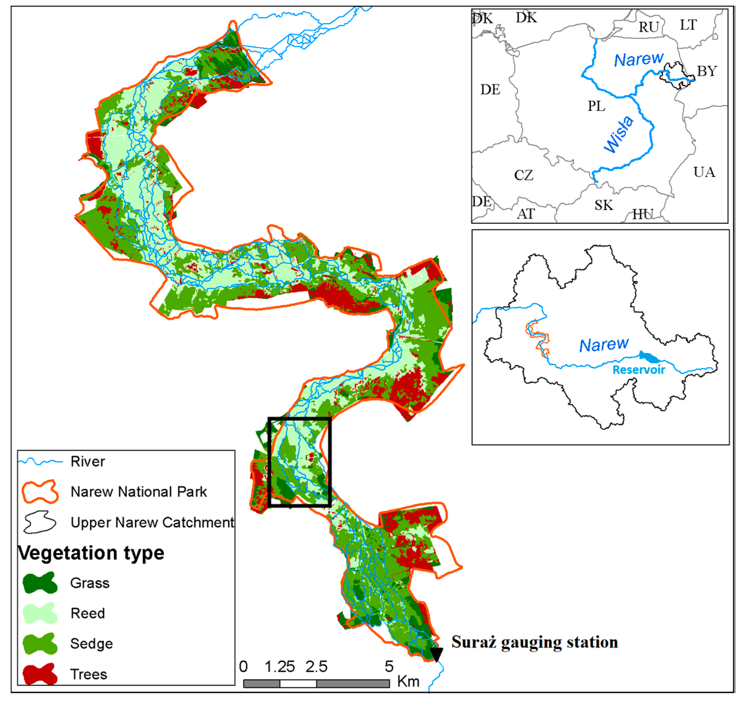
The Upper River Narew is a lowland, low-gradient river situated in northeastern Poland (Figure 1). The river valley, due to its precious environmental nature, has also been designated a Wetland of International Importance under the terms of the RAMSAR Convention and is protected as a part of Natura 2000 (Bird and Habitat directive) and the Narew National Park (NNP). Within the NNP borders, the river consists of a complex network of small interconnected, unconfined channels draining peat substrate. The riparian corridor vegetation structure is dominated by reed communities (Phragmition) occupying 35% and sedge communities (Magnocaricion) also covering 35% of the valley. Mature trees and scrubs (Alnetea glutinosae) cover 15% of the NNP area mostly at the edges of the valley and the remaining 15% is occupied by grass (Molinio-Arrhenatheretea) (Figure 1). The uppermost reach of the Narew catchment was dammed and a reservoir with total capacity of 79.5 million m3 was constructed (Figure 1). The reservoir, which has operated since 1992, caused changes in extreme flow events, increasing low and decreasing high flows [61].
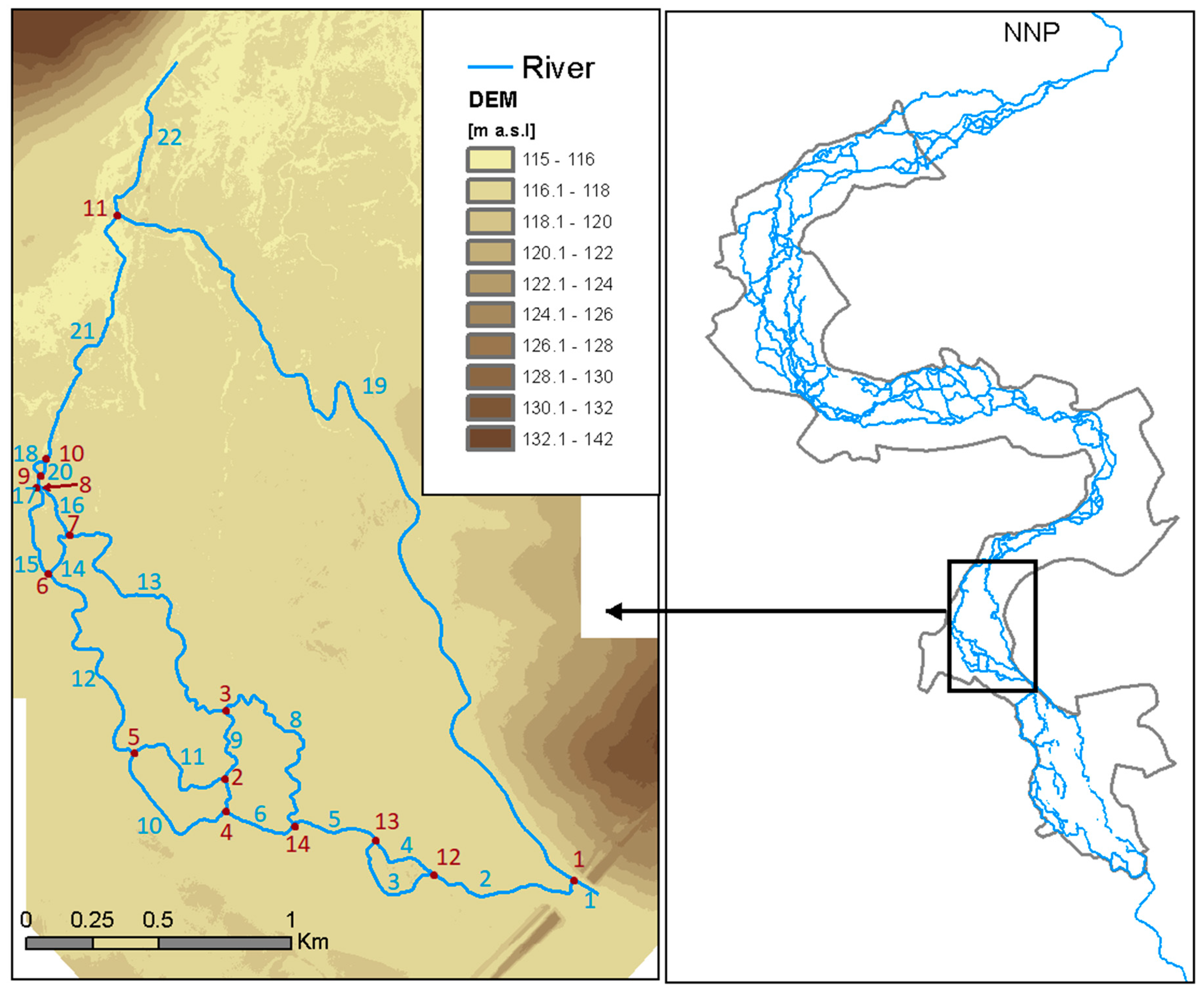
The study focused on a 4-km long stretch of the anastomosing river section in the NNP (Figure 2). The analyzed reach is characterized by low gradient (0.0002 m·m−1) and mean annual discharge (1951–2016) recorded at the Suraż gauging, located upstream of the analyzed section, equal to 15.5 m3·s−1. Average width/depth ratio is very low and equals 2. According to long-term records of sediment concentrations monitored at the Suraż water quality monitoring point, average concentration of sediment equals 19 mg·L−1.
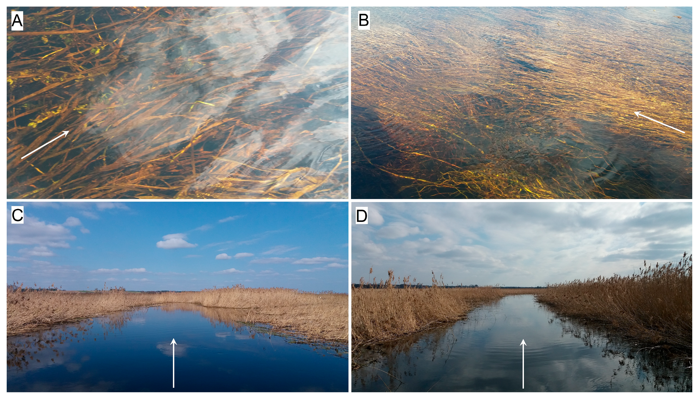
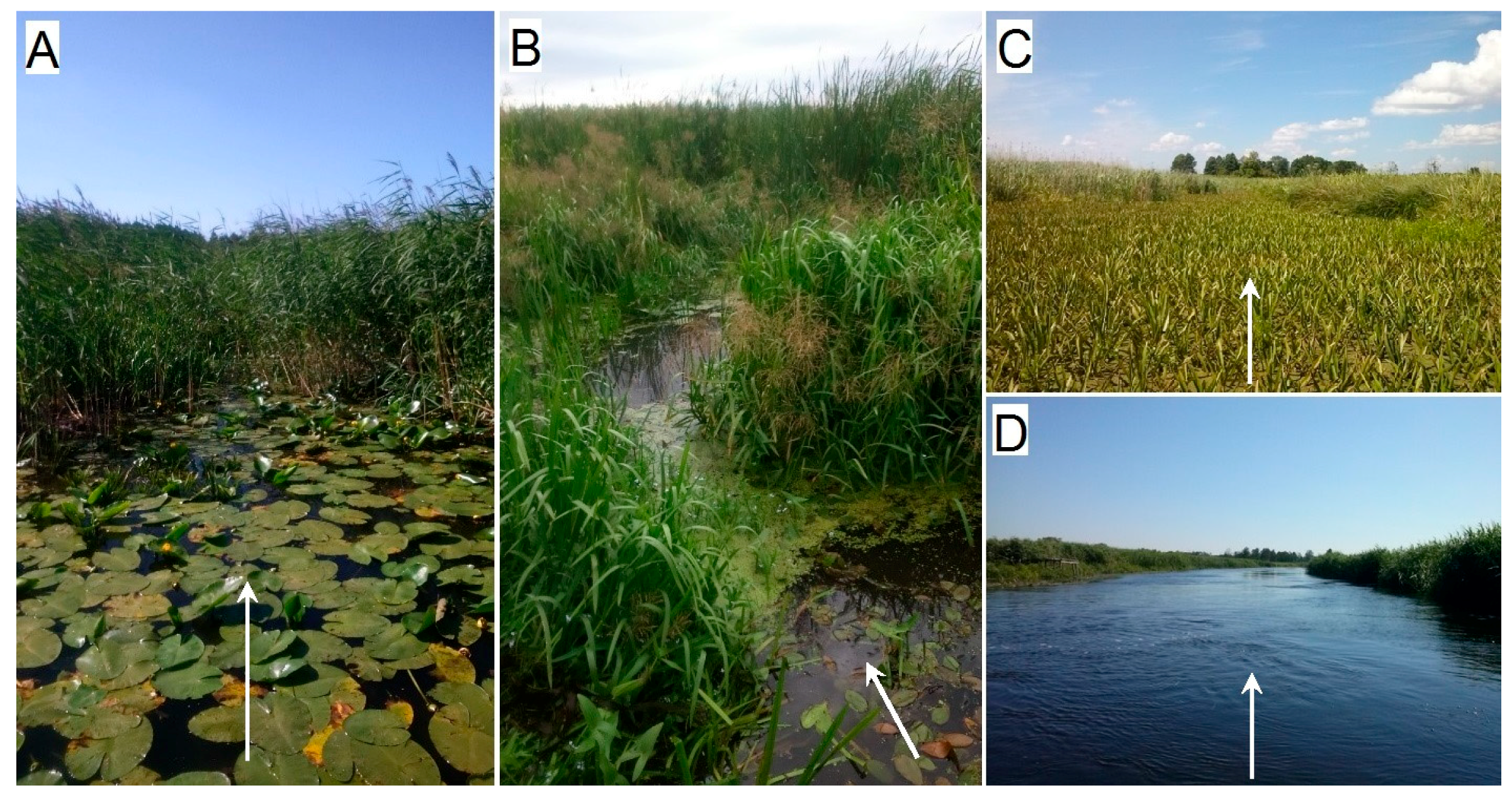
In the NNP, the abundance of aquatic vegetation in the river channels strongly depends on the water depth and current velocity. Active channels deeper than 2 m are usually free of vegetation (Figure 3C,D and Figure 4D) but shallower reaches are extensively colonized by both emergent and submerged macrophytes (Figure 3A,B and Figure 4A–C). It is worth stating that in-stream vegetation in the analyzed area densely overgrows channels not only during the summer season, but also survives to some extent the dormancy season, influencing the hydraulics of channels for the whole year.
Studies show that in recent decades uncontrolled expansion of common reed (Phragmites australis) became a serious problem causing significant loss of biodiversity [62] and the loss of anabranches [61,63,64]. Therefore, a special focus on a detailed recognition of flow conditions, improving the mechanistic understanding of anastomosing in lowland river floodplains and facilitating the development of sustainable conservation strategies for these important habitats is required.
2.2. Fieldwork and Modeling Tool
Broad field measurements conducted for the purpose of this research included discharge measurements at all 14 confluences and channel geometry as well as water level measurements using GPS (76 cross-sections). Cross-sections of all river reaches were measured at every inlet and outlet part and additionally every 500 m. Discharge measurements were conducted in two different periods: (1) during bankfull water stages in the dormancy season (16 m3·s−1); and (2) during low water stages in growing season (7 m3·s−1). This ensured the recognition of different in-stream vegetation conditions varying between the seasons. In both cases, only river flows below bankfull stages were considered.
In this study, a one-dimensional steady flow model developed in the MATLAB computing environment, hereafter referred to as Multi-Channel Flow Routing Model (MFRM), was used. The rationale for developing a new model instead of using existing ones was that none of the available ones were equipped with automatic optimization procedure of the roughness parameters. Whilst in single channel systems this procedure is relatively simple and manually feasible, in complex interconnected system of channels it becomes difficult and laborious. While the full description of model setup, calibration and validation was presented in the study of Marcinkowski et al. [65], here we provide a brief overview, important in the context of the main goal of this paper.
MFRM operates under the following assumptions: (1) steady flow conditions; (2) one-dimensional flow is considered, where only the velocity components in the flow direction are taken into account, and the elevation of the energy line is the same in the whole cross-section; (3) river flow can be expressed in terms of energy conservation equation; (4) discharge within each river branch is uniform; and (5) flow is subcritical. Manning’s roughness coefficients were used to describe the flow resistance resulting from vegetation presence in the channel. It was assumed that each channel can be characterized with a single value of the coefficient. Floodplain roughness was not considered, as only channel flows were investigated (below bankfull stages). The stationarity of the model required elaborating two different sets of Manning’s coefficients: (1) for highly vegetated growing season; and (2) for less intensively vegetated dormancy season.
The model was calibrated and validated to minimize the difference between calculated and observed water levels at every channel junction of the analyzed river system, ensuring that computed water energy heads at parallel anabranches are equal (at channel splitting junctions). Manning’s coefficients were determined using the automatic optimization procedure minimizing the difference in water energy levels between branches and measurements.
2.3. Model Performance
Manning’s coefficients in MFRM for all river branches ranged from 0.027 m−1/3·s to 0.054 m−1/3·s (0.040 m−1/3·s on average) and from 0.027 m−1/3·s to 0.089 m−1/3·s (0.061 m−1/3·s on average) for dormancy and growing season, respectively. It appears to be reasonable comparing those values with the literature [66,67,68]. The overall assessment of model accuracy can be expressed by average differences in: (1) simulated water levels, which for bot, growing and dormancy seasons did not exceed 6.6 cm comparing to measured water levels; and (2) energy level between branches which reached accuracy at 10−5 m level (Table 1).
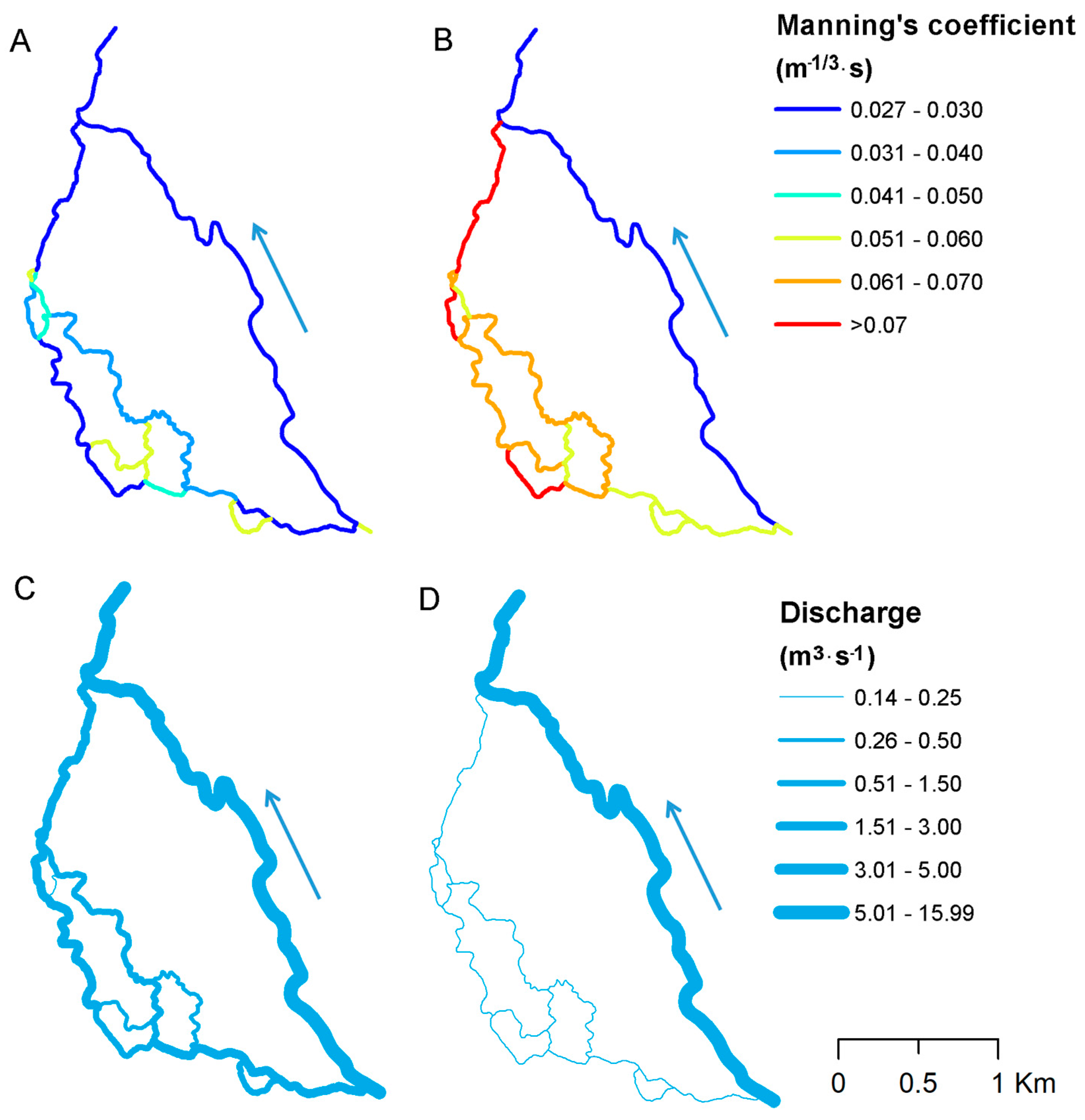
Figure 5A,B presents the spatial variability of MFRM Manning’s coefficients for two separate vegetation conditions. As expected, on the left-hand side of the valley, Manning’s coefficients are greater, which is caused by channels’ shallow geometry and the vegetation blockage rate, i.e., height of vegetation (H) either equal to water depth (h) (h/H = 1) (cf. Figure 3A,B) or higher than water depth (h/H < 1) (cf. Figure 3A–C), overgrowing the whole channel width. For the main channel (cf. Figure 3C,D and Figure 4D), on the right-hand side, this value is significantly lower, as the blockage rate is significantly lower. Although the Manning’s coefficients differ between seasons (greater values in growing season), similar spatial variation is maintained in both seasons. Water flow distribution determined by vegetation resistance significantly differs between seasons. During the winter season, when mean water flow equals 16 m3·s−1 nearly 20% (3.1 m3·s−1) is contributed into side anabranches (Figure 5C), whereas, in the summer season, with mean flow 7 m3·s−1, the contribution rate decreases to only 2% (0.17 m3·s−1) (Figure 5D).
2.4. Model Sensitivity Analysis
The sensitivity analysis of MFRM on vegetation changes was calculated based on the central difference formula (Equation (1)) [56].
where θj stands for the Manning coefficient for j-th channel branch, ∆θj is the change of the Manning’s coefficient value, and Q is the discharge for all river branches as model output.
It was assessed iteratively by altering the Manning’s coefficient (by 0.005 m−1/3·s) in one branch at a time and launching the model computations. The relative coefficient change was tested for both growing season and dormancy season. Finally, sensitivity results were presented in relation to maximum discharge change, and hence, they ranged between 0 and 1.
2.5. Vegetation Changes Impact on Water Flow
To analyze the impact of in-channel vegetation changes on water flow distribution, plants, along with the degree of their abundance in the channel, were grouped based on their physical parameters (height and width), which determine the blockage factor (the fraction of the channel cross-section blocked by vegetation) [69]. As proven by Luhar and Nepf [70], the Manning roughness coefficient due to vegetation depends primarily on the blockage factor. Nepf [66] in her studies showed also that resistance to flow in channels with vegetation is influenced primarily by plants’ submergence. The empirical nature of the Manning’s equation has often been criticized, but it remains in wide use [40,42,49,51,52,53]. Even though the most fundamental treatments link resistance coefficients to channel boundary roughness, representing many sources of flow resistance (i.e., vegetation) by such coefficients has been practiced for decades [67]. To each group of vegetation, Manning’s coefficient value was assigned after Arcement and Schneider [68] and Rhee et al. [71] (Table 2). Afterwards, for the reaches with highest flow resistance (>0.05 m−1/3·s) (cf. Figure 5B), two different variants reflecting potential man-made interventions (i.e., mowing) in channel vegetation structure were tested in MFRM. After changing uniformly the Manning’s coefficient values in aforementioned reaches to 0.05 m−1/3·s for summer season (which means absence of emergent vegetation) and 0.025 m−1/3·s for both seasons (which means absence of submerged vegetation along the channel bottom), discharge distribution was recalculated and compared with the calibrated variant.
3. Results
3.1. Model Sensitivity Analysis
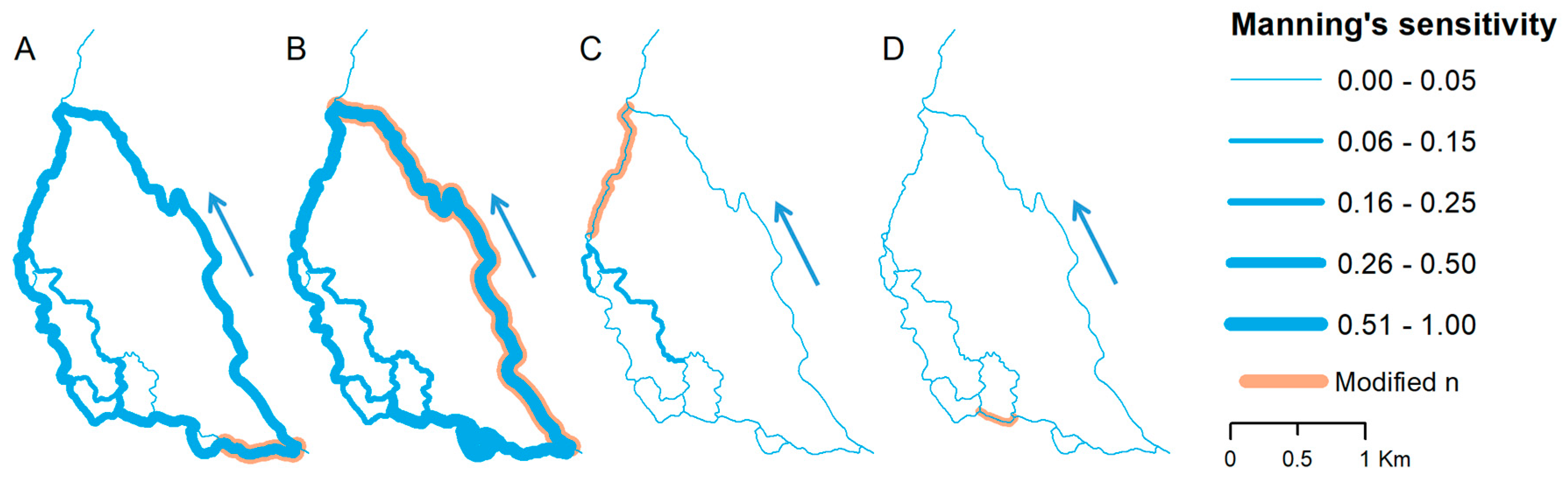
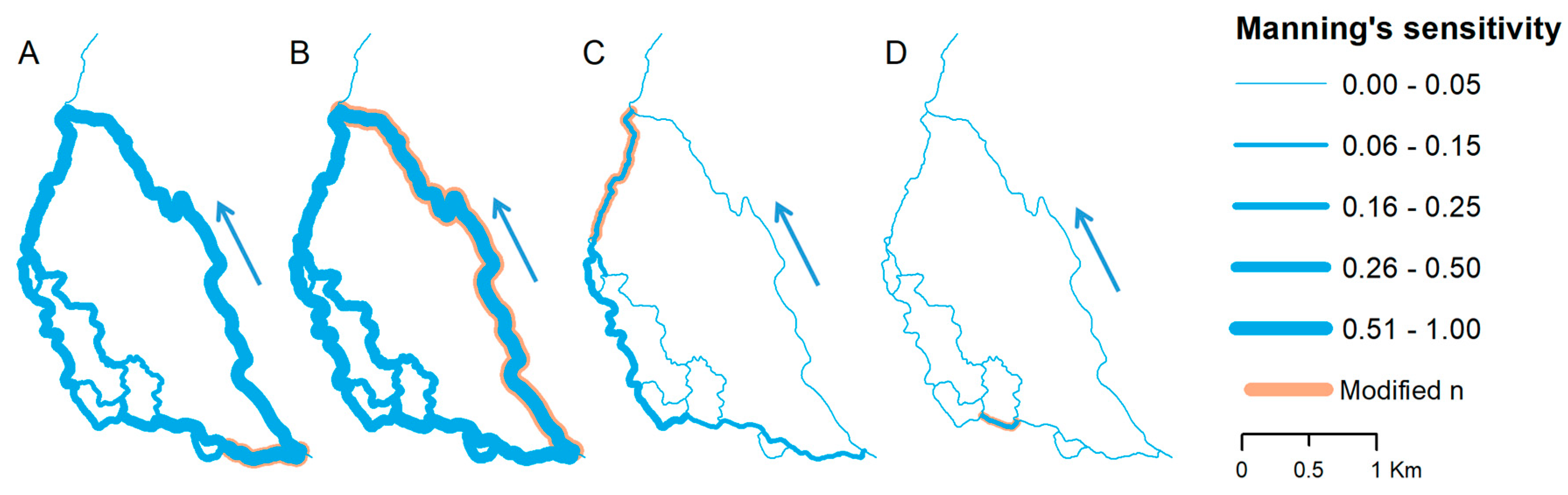
The results of MFRM sensitivity analysis induced by Manning’s coefficient alteration are diverse in both magnitude and spatial distribution. There is also a considerable seasonal difference noted, with general higher discharge changes in the summer season (18% on average) compared to winter season (6% on average). In Figure 6 and Figure 7, model sensitivity to Manning’s coefficient changes for selected anabranches and their impact on water flow are presented. Although Manning’s coefficient changes were tested for all 22 river reaches, only selected cases are shown, which represent characteristic groups of sensitivity (high, moderate and low). As shown, the model response is varied and strongly depends on location of change. The highest sensitivity is noted for reaches at the first confluence (Figure 6A,B and Figure 7A,B), where flow is distributed between main channel and side anabranches. Manning’s coefficient changes in left-hand side reach (Figure 6A and Figure 7A) significantly alters flow in further downstream side branches, but also in the main channel. Similar response is noted for change of Manning’s coefficient in the main channel (Figure 6B and Figure 7B). Much lower sensitivity is noted for downstream side anabranches (Figure 6C and Figure 7C) in which Manning’s coefficient changes moderately affected river flow in part of the upstream reaches excluding main channel. There were also situations, especially for short (less than 500 m) reaches, with no impact on water flow noted (Figure 6D and Figure 7D).
3.2. Impact of Vegetation Changes on Water Flow Distribution
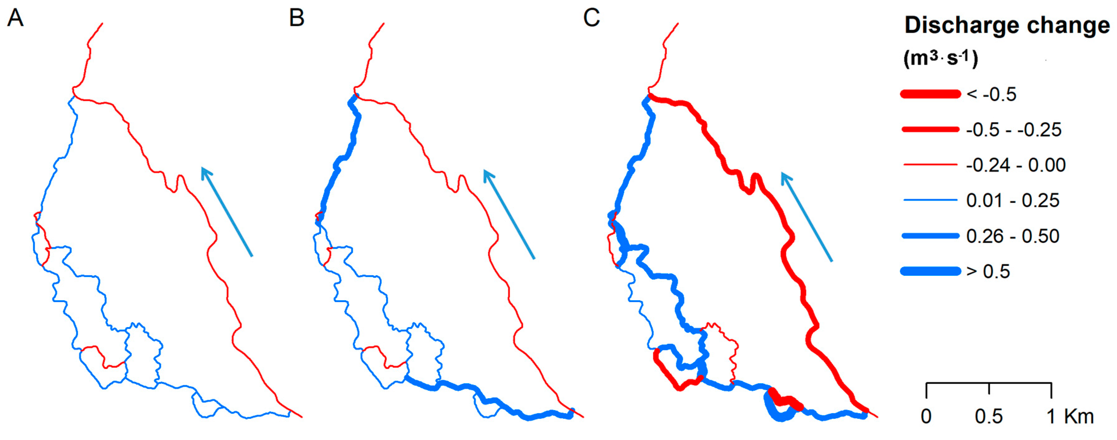
Simulation of vegetation from Group 2 (cf. Table 2) indicated moderate impact on water flow distribution (Figure 8A). Following sensitivity analysis results (Figure 6A,C), Manning’s coefficient changes in all left-hand side anabranches affected flow distribution in all reaches, including the main channel. Generally, it resulted in redirection of flow by 0.2 m3·s−1 to side anabranches at the expense of the main channel. Although the change might be assumed as low, compared to average flow conditions in summer season (0.17 m3·s−1), the contribution was more than doubled. Going further, simulation of vegetation from group (cf. Table 1) intensified the response. The simulation results indicate an overall increase of water flow contribution by 0.5 m3·s−1, which is three-fold higher than observed during the summer season (Figure 8B).
The results observed for winter conditions are similar in terms of spatial distribution but slightly higher considering the magnitude of change. An overall increase by 0.6 m3·s−1 was observed which was unequally redistributed between the side anabranches (Figure 8C). Although the total redistribution rate for winter conditions is higher compared to summer season, the relative change is significantly lower. For summer conditions, the flow increase reached 400%, whereas for winter conditions only 15%. It means that the impact of vegetation on flow distribution in analyzed anastomosing section is significantly higher in growing season.
It is worth stating that uniform change of Manning’s coefficient in all side anabranches does not ensure the homogenous response in terms of water flow. As can be noted in Figure 8 for some reaches Manning’s coefficient decrease resulted in flow decrease. Moreover, the response varies not only between certain reaches but also between seasons. It proves the complex nature of the system of interconnected channels that is strongly determined by resistance phenomena caused by in-channel vegetation in the first instance, and also by channels geometry (width and depth).
4. Discussion
Among studies concerning multi-channel rivers, braided patterns substantially prevail over anastomosing, leaving the latter poorly investigated. This study aimed at assessing the impact of in-stream vegetation on water flow distribution in the anastomosing river system, using a 1D steady-flow model. As stated by Kale et al. [72], the splitting discharge ratio at a bifurcation might be highly asymmetric due to changes in the planform and section of a river network. Following this assumption, Van et al. [32] developed a 1D steady-flow model for anastomosing section of the River Mekong, where measured discharge data entering each individual channel was not available. They used simple symmetry ratio to estimate the division of discharge at the bifurcations, based on the cross-sectional wetted areas of the splitting channels downstream of the bifurcation node. During the optimization procedure, they adjusted Manning’s coefficient to obtain compatibility in water energy levels. It has to be noted that splitting rule based exclusively on the geometry (wetted area) is highly uncertain as it does not take into account vegetation drag force, which also controls the volume of water flowing into the channel. Here, the MFRM is optimized using actual measured entry discharge into each single channel of the complex anastomosing system, which is a significant advantage of this study. Gibson and Pasternack [33] developed a 1D model for anastomosing reach of the River Yuba where only one bifurcation was modeled. With no measurements on discharge division between the channels, the authors found 1D model simulations underwhelming and split flow modeling to be complex. In both studies, Manning’s coefficient was used to describe channel roughness. Moreover, Van et al. [32] used Manning’s coefficient to estimate the impact of different land cover change scenarios on water flow. Similar to this study, they used fixed Manning’s values for different types of vegetation based on the literature and examined its influence on water flow. To our best knowledge, this study was the first that optimized the water flow model in multi-channel river system, based on the broad field measurements, i.e., channel cross-sections, water levels, entry discharges and in-situ vegetation mapping. Detailed fieldwork reduced the uncertainty of the results [50] and made them more reliable for further works. Although it was reported by Merwade et al. [73] that 1D hydraulic models are not suitable to model the detailed hydraulics of multi-channel rivers, the MFRM applied in this study helped to identify impact of vegetation on flow distribution, from which a more comprehensive hydraulic model could be constructed.
Manning’s equation used in this study is widely accepted methodology in stream resistance evaluation, especially in vegetated areas [46], and was successfully incorporated in numerous researches investigating the impact of vegetation on water flow, depth and velocity [32,33,47,48]. A quantitative comparison of calibrated Manning’s coefficient values with those reported in the literature can be made, linking plant traits (height and flexibility) to roughness. Shields et al. [67] gathered in their study various methods of Manning’s coefficient estimation for rigid [74,75,76] and flexible plants [77,78] differentiating their values based on plant height (H) and flow depth (h). In the MFRM, reaches where rigid plants were mapped in the field (Figure 4A–C), characterized by height ratio 0.5 < h/H < 1, calibrated Manning’s coefficient varied between 0.04 m−1/3·s and 0.06 m−1/3·s, which is in agreement with the literature (0.03 m−1/3·s–0.06 m−1/3·s) [74,75,76]. Reaches with flexible vegetation mapped in the field (Figure 3A,B), characterized by height ratio h/H = 1 varied between 0.07 m−1/3·s and 0.09 m−1/3·s, which is comparable with the results presented by Jarvela (0.07 m−1/3·s) [78] and Whittaker et al. (0.08 m−1/3·s) [77]. Methods compared by Shields et al. [67] differ in methodology but in general are all supported by field measurements, and therefore their results in most cases make physical sense [67]. Thus, optimized values of Manning’s coefficient presented in this study can be assumed reasonable for different plant traits mapped in the field. Comparing the seasonal changes of Manning’s coefficient, there is a notable difference between winter and summer season. Similar to study by Song et al. [46], roughness condition is significantly higher in summer compared to winter season. Therefore, the development of models for two different vegetational conditions presented in this study was justified, to capture the seasonal variations in flow conditions determined by the in-channel vegetation.
The impact of vegetation on anastomosing system flow characteristics is to date recognized mainly in theory [20,22,26,27,28]. According to theoretical understanding, vegetation encroachment causes flow velocity decrease and sediment aggradation, which initiates feedback mechanisms involving further invasion of aquatic plants in the channel and water loss [26,27,28]. Marcinkowski et al. [63] recognized that anabranches loss in the anastomosing section of the River Narew is periodically triggered during the summer low flow conditions, when water discharge in the anabranches promotes sediment vertical accretion. Other studies on anastomosing rivers functioning indicate that localized flow blockages caused by vegetation are one of the key factors controlling their formation [20,22]. Therefore, it can be assumed that the most important factors controlling anabranches maintenance and persistence are related to water and sediment supply. This study, although not incorporating sediment routing, to our best knowledge, is the first that described quantitatively flow distribution under diverse vegetational conditions, using mathematical modeling. Complex system of splitting and rejoining channels of anastomosing river system responses differently to vegetation obstacles than single-channel river. In single-channel rivers flow blockage caused by in-channel vegetation decreases flow velocity and increases water levels, however, water volume flowing through the channel remains constant. In anastomosing rivers, any flow blockage increasing water levels causes impoundment effect upstream to bifurcation node where the flow splits. Subsequently, according to Bernoulli’s conservation equation (for details of use in MFRM, see Marcinkowski et al. [65]), a certain volume of water is redirected from one channel (highly vegetated) to another (less vegetated). Therefore, flow distribution at each bifurcation in the anastomosing river depends on the channels geometry [72] and in-channel vegetation characteristics (e.g., height and density) determining their drag force [66]. Model results proved that the impact of vegetation changes under winter flow/vegetation conditions is significantly lower than under summer conditions during growing season. A great advantage of this study is that the MFRM allows to calculate flow redistribution in the entire river system as a response to vegetation changes in particular channels.
Author Contributions
Conceptualization, P.M., A.K. and T.O.; Methodology, P.M., A.K. and T.O.; Software, P.M. and A.K.; Formal Analysis, P.M.; Investigation, P.M.; Writing—Original Draft Preparation, P.M.; Writing—Review and Editing, T.O.; Visualization, P.M.; and Supervision, A.K. and T.O.
Funding
This research was financed by the National Science Centre, Poland under grant agreement 2015/19/N/ST10/01629.
Acknowledgments
We would like to thank two anonymous Reviewers for their comments and suggestions, which helped to improve the manuscript.
Conflicts of Interest
The authors declare no conflict of interest.
References
- Gurnell, A. Plants as river system engineers: Further comments. Earth Surf. Process. Landf. 2014, 40, 135–137. [Google Scholar] [CrossRef]
- Gurnell, A.M.; Corenblit, D.; García de Jalón, D.; González del Tánago, M.; Grabowski, R.C.; O’Hare, M.T.; Szewczyk, M. A conceptual model of vegetation-hydrogeomorphology interactions within river corridors. River Res. Appl. 2016, 32, 142–163. [Google Scholar] [CrossRef]
- Schoelynck, J.; Creëlle, S.; Buis, K.; De Mulder, T.; Emsens, W.; Hein, T.; Meire, D.; Meire, P.; Okruszko, T.; Preiner, S.; et al. What is a macrophyte patch? Patch identification in aquatic ecosystems and guidelines for consistent delineation. Ecohydrol. Hydrobiol. 2017, 18, 1–9. [Google Scholar] [CrossRef]
- Zong, L.; Nepf, H. Spatial distribution of deposition within a patch of vegetation. Water Resour. Res. 2011, 47, 1–12. [Google Scholar] [CrossRef]
- Solari, L.; Van Oorschot, M.; Belletti, B.; Hendriks, D.; Rinaldi, M.; Vargas-Luna, A. Advances on modelling riparian vegetation-hydromorphology interactions. River Res. Appl. 2016, 2, 164–178. [Google Scholar] [CrossRef]
- Verschoren, V.; Meire, D.; Schoelynck, J.; Buis, K.; Bal, K.D.; Troch, P.; Meire, P.; Temmerman, S. Resistance and reconfiguration of natural flexible submerged vegetation in hydrodynamic river modelling. Environ. Fluid Mech. 2016, 16, 245–265. [Google Scholar] [CrossRef] [Green Version]
- Corenblit, D.; Baas, A.C.W.; Bornette, G.; Darrozes, J.; Delmotte, S.; Francis, R.A.; Gurnell, A.M.; Julien, F.; Naiman, R.J.; Steiger, J. Feedbacks between geomorphology and biota controlling Earth surface processes and landforms: A review of foundation concepts and current understandings. Earth Sci. Rev. 2011, 106, 307–331. [Google Scholar] [CrossRef]
- Gurnell, A. Plants as river system engineers. Earth Surf. Process. Landf. 2014, 39, 4–25. [Google Scholar] [CrossRef]
- Vaughan, I.P.; Diamond, M.; Gurnell, A.M.; Hall, K.A.; Jenkins, A.; Milner, N.J.; Naylor, L.A.; Sear, D.A.; Woodward, G.; Ormerod, S.J. Integrating ecology with hydromorphology: A priority for river science and management. Aquat. Conserv. Mar. Freshw. Ecosyst. 2009, 19, 113–125. [Google Scholar] [CrossRef]
- Oorschot, M.; Kleinhans, M.; Geerling, G.; Middelkoop, H. Distinct patterns of interaction between vegetation and morphodynamics. Earth Surf. Process. Landf. 2016, 41, 791–808. [Google Scholar] [CrossRef]
- Schuurman, F.; Marra, W.A.; Kleinhans, M.G. Physics-based modeling of large braided sand-bed rivers: Bar pattern formation, dynamics, and sensitivity. J. Geophys. Res. Earth Surf. 2013, 118, 2509–2527. [Google Scholar] [CrossRef] [Green Version]
- Lotsari, E.; Wainwright, D.; Corner, G.D.; Alho, P.; Käyhkö, J. Surveyed and modelled one-year morphodynamics in the braided lower Tana River. Hydrol. Process. 2013, 28, 2685–2716. [Google Scholar] [CrossRef]
- Williams, R.D.; Brasington, J.; Hicks, M.; Measures, R.; Rennie, C.D.; Vericat, D. Hydraulic validation of two-dimensional simulations of braided river flow with spatially continuous aDcp data. Water Resour. Res. 2013, 49, 5183–5205. [Google Scholar] [CrossRef] [Green Version]
- Nicholas, A. Morphodynamic diversity of the world’s largest rivers. Geology 2013, 41, 475–478. [Google Scholar] [CrossRef]
- Bertoldi, W.; Siviglia, A.; Tettamanti, S.; Toffolon, M.; Vetsch, D.; Francalanci, S. Modeling vegetation controls on fluvial morphological trajectories. Geophys. Res. Lett. 2014, 41, 7167–7175. [Google Scholar] [CrossRef] [Green Version]
- Williams, R.D.; Brasington, J.; Hicks, D.M. Numerical modelling of braided river morphodynamics: Review and future challenges. Geogr. Compass 2016, 10, 102–127. [Google Scholar] [CrossRef]
- Jowett, J.G.; Duncan, M.J. Effectiveness of 1D and 2D hydraulic models for instream habitat analysis in a braided river. Ecol. Eng. 2012, 48, 92–100. [Google Scholar] [CrossRef]
- Nanson, G.C.; Croke, J.C. A genetic classification of floodplains. Geomorphology 1992, 4, 459–486. [Google Scholar] [CrossRef] [Green Version]
- Nanson, G.C.; Knighton, A.D. Anabranching rivers: Their cause, character and classification. Earth Surf. Process. Landf. 1996, 21, 217–239. [Google Scholar] [CrossRef]
- Gradziński, R.; Baryła, J.; Doktor, M.; Gmur, D.; Gradziński, M.; Kędzior, A.; Paszkowski, M.; Soja, R.; Zieliński, T.; Żurek, S. Vegetation-controlled modern anastomosing system of the upper Narew River (NE Poland) and its sediments. Sediment. Geol. 2003, 157, 253–276. [Google Scholar] [CrossRef]
- Makaske, B.; Lavooi, E.; de Haas, T.; Kleinhans, M.G.; Smith, D.G. Upstream control of river anastomosis by sediment overloading, upper Columbia River, British Columbia, Canada. Sedimentology 2017, 64, 1488–1510. [Google Scholar] [CrossRef] [Green Version]
- McCarthy, T.S.; Ellery, W.N.; Stanistreet, I.G. Avulsion mechanisms on the Okavango fan, Botswana: The control of a fluvial system by vegetation. Sedimentology 1992, 39, 779–795. [Google Scholar] [CrossRef]
- Schumann, R.R. Morphology of Red Creek, Wyoming, an arid-region anastomosing channel system. Earth Surf. Process. Landf. 1989, 14, 277–288. [Google Scholar] [CrossRef]
- Smith, N.D.; Cross, T.A.; Dufficy, J.; Clough, S.R. Anatomy of avulsion. Sedimentology 1989, 36, 1–23. [Google Scholar] [CrossRef]
- Tooth, S.; Nanson, G.C. The role of vegetation in the formation of anabranching channels in an ephemeral river, Northern plains, arid central Australia. Hydrol. Process. 2000, 14, 3099–3117. [Google Scholar] [CrossRef]
- McCarthy, T.S.; Ellery, W.N.; Rogers, K.H.; Cairncross, B.; Ellery, K. The roles of sedimentation and plant growth in changing flow patterns in the Okavango Delta, Botswana. S. Afr. J. Sci. 1986, 82, 579–585. [Google Scholar]
- Ellery, W.N.; Ellery, K.; Rogers, K.H.; McCarthy, T.S.; Walker, B.H. Vegetation, hydrology and sedimentation processes as determinants of channel form and dynamics in the northeastern Okavango Delta, Botswana. Afr. J. Ecol. 1993, 31, 10–25. [Google Scholar] [CrossRef]
- Stanistreet, I.G.; Cairncross, B.; McCarthy, T.S. Low sinuosity and meandering bedload rivers of the Okavango Fan: Channel confinement by vegetated levées without fine sediment. Sediment. Geol. 1993, 85, 135–156. [Google Scholar] [CrossRef]
- Wende, R.; Nanson, G.C. Anabranching rivers: Ridge-form alluvial channels in tropical northern Australia. Geomorphology 1998, 22, 205–224. [Google Scholar] [CrossRef]
- Tabata, K.K.; Hickin, E.J. Intrachannel hydraulic geometry and hydraulic efficiency of the anastomosing Columbia river, southeastern British Columbia, Canada. Earth Surf. Process. Landf. 2003, 28, 837–852. [Google Scholar] [CrossRef]
- Jansen, J.D.; Nanson, G.C. Anabranching and maximum flow efficiency in Magela Creek, northern Australia. Water Resour. Res. 2004, 40, W04503. [Google Scholar] [CrossRef]
- Van, T.P.D.; Carling, P.A.; Atkinson, P.M. Modelling the bulk flow of a bedrock-constrained, multi-channel reach of the Mekong River, Siphandone, southern Laos. Earth Surf. Process. Landf. 2012, 37, 533–545. [Google Scholar] [CrossRef]
- Gibson, S.A.; Pasternack, G.B. Selecting between one-dimensional and two-dimensional hydrodynamic models for ecohydraulic analysis. River Res. Appl. 2016, 32, 1365–1381. [Google Scholar] [CrossRef]
- Romanowicz, R.; Kiczko, A.; Napiórkowski, J. Stochastic transfer function simulator of a 1-D flow routing. Publ. Inst. Geophys. Pol. Acad. Sci. 2008, E-10, 151–160. [Google Scholar]
- Romanowicz, R.; Kiczko, A.; Napiórkowski, J. Stochastic transfer function model applied to combined reservoir management and flow routing. Hydrol. Sci. J. 2010, 55, 27–44. [Google Scholar] [CrossRef]
- Mashriqui, H.S.; Halgren, J.S.; Reed, S.M. 1D river hydraulic model for operational flood forecasting in the tidal Potomac: Evaluation for freshwater, tidal, and wind-driven events. J. Hydraul. Eng. 2014, 140, 04014005. [Google Scholar] [CrossRef]
- Horritt, M.S.; Bates, P.D. Evaluation of 1D and 2D numerical models for predicting river flood inundation. J. Hydrol. 2002, 268, 87–99. [Google Scholar] [CrossRef]
- Jordanova, A.A.; James, C.S. Experimental study of bed load transport through emergent vegetation. J. Hydraul. Eng. 2003, 129, 474–478. [Google Scholar] [CrossRef]
- Wilson, C.A.M.E. Flow resistance models for flexible submerged vegetation. J. Hydrol. 2007, 342, 213–222. [Google Scholar] [CrossRef]
- Abu-Aly, T.R.; Pasternack, G.B.; Wyrick, J.R.; Barker, R.; Massa, D.; Johnson, T. Effects of LiDAR-derived, spatially distributed vegetation roughness on two-dimensional hydraulics in a gravel-cobble river at flows of 0.2 to 20 times bankfull. Geomorphology 2014, 206, 468–482. [Google Scholar] [CrossRef] [Green Version]
- Curran, J.W.; Hession, W.C. Vegetative impacts on hydraulics and sediment processes across the fluvial system. J. Hydrol. 2013, 505, 364–376. [Google Scholar] [CrossRef]
- Manners, R.; Schmidt, J.; Wheaton, J.M. Multiscalar model for the determination of spatially explicit riparian vegetation roughness. J. Geophys. Res. Earth Surf. 2013, 118, 65–83. [Google Scholar] [CrossRef] [Green Version]
- Bywater-Reyes, S.; Diehl, R.M.; Wilcox, A.C. The influence of a vegetated bar on channel-bend flow dynamics. Earth Surf. Dynam. 2018, 6, 487–503. [Google Scholar] [CrossRef]
- Baptist, M.J.; Van Den Bosch, L.V.; Dijkstra, J.T.; Kapinga, S. Modelling the effects of vegetation on flow and morphology in rivers. Large Rivers 2003, 15, 339–357. [Google Scholar] [CrossRef]
- James, C.; Birkhead, A.; Jordanova, A. Flow resistance of emergent vegetation. J. Hydraul. Res. 2004, 42, 390–398. [Google Scholar] [CrossRef] [Green Version]
- Song, S.; Schmalz, B.; Xu, Y.P.; Fohrer, M. Seasonality of roughness—The indicator of annual river flow resistance condition in a lowland catchment. Water Resour. Manag. 2017, 31, 3299–3312. [Google Scholar] [CrossRef]
- O’Hare, M.T.; McGahey, C.; Bissett, N.; Cailes, C.; Henville, P.; Scarlett, P. Variability in roughness measurements for vegetated rivers near base flow, in England and Scotland. J. Hydrol 2010, 385, 361–370. [Google Scholar] [CrossRef]
- Parhi, P.K.; Sankhua, R.; Roy, G.P. Calibration of channel roughness for Mahanadi River, (India) using HEC-RAS model. J. Water Resour. Prot. 2012, 4, 847–850. [Google Scholar] [CrossRef]
- Yang, T.H.; Wang, Y.C.; Tsung, S.C.; Guo, W.D. Applying micro-genetic algorithm in the one-dimensional unsteady hydraulic model for parameter optimization. J. Hydroinform. 2014, 16, 772–783. [Google Scholar] [CrossRef]
- Frias, C.E.; Abad, J.D.; Mendoza, A.; Paredes, J.; Ortals, C.; Montoro, H. Planform evolution of two anabranching structures in the Upper Peruvian Amazon River. Water Resour. Res. 2015, 51, 2742–2759. [Google Scholar] [CrossRef] [Green Version]
- Green, J. Effect of macrophyte spatial variability on channel resistance. Adv. Water Resour. 2006, 29, 426–438. [Google Scholar] [CrossRef]
- Kiczko, A.; Romanowicz, R.J.; Osuch, M.; Karamuz, E. Maximising the usefulness of flood risk assessment for the river vistula in warsaw. Nat. Hazards Earth Syst. Sci. 2013, 13, 3443–3455. [Google Scholar] [CrossRef]
- Romanowicz, R.J.; Kiczko, A. An event simulation approach to the assessment of flood level frequencies: Risk maps for the Warsaw reach of the river Vistula. Hydrol. Process. 2016, 30, 2451–2462. [Google Scholar] [CrossRef]
- De Doncker, L.; Troch, P.; Verhoeven, R.; Buis, K. Deriving the relationship among discharge, biomass and Manning’s coefficient through a calibration approach. Hydrol. Process. 2011, 25, 1979–1995. [Google Scholar] [CrossRef]
- Pappenberger, F.; Beven, K.; Morrit, H.; Blazkova, S. Uncertainty in the calibration of effective roughness parameters in hec-ras using inundation and downstream level observations. J. Hydrol. 2005, 302, 46–69. [Google Scholar] [CrossRef]
- De Pauw, D.J.W.; Vanrolleghem, P.A. Practical aspects of sensitivity function approximation for dynamic models. Math. Comput. Model. Dyn. Syst. 2006, 12, 395–414. [Google Scholar] [CrossRef]
- Haaker, M.P.R.; Verheijen, P.J.T. Local and global sensitivity analysis for a reactor design with parameter uncertainty. Chem. Eng. Res. Des. 2004, 82, 591–598. [Google Scholar] [CrossRef]
- Morio, J. Global and local sensitivity analysis methods for a physical system. Eur. J. Phys. 2011, 32, 1577–1583. [Google Scholar] [CrossRef]
- Wright, K.A.; Goodman, D.H.; Som, N.A.; Alvarez, J.; Martin, A.; Hardy, T.B. Improving hydrodynamic modelling: An analytical framework for assessment of two-dimensional hydrodynamic models. River Res. Appl. 2017, 33, 170–181. [Google Scholar] [CrossRef]
- Neal, J.C.; Odoni, N.A.; Trigg, M.A.; Freer, J.E.; Garcia-Pintado, J.; Mason, D.C.; Wood, M.; Bates, P.D. Efficient incorporation of channel cross-section geometry uncertainty into regional and global scale flood inundation models. J. Hydrol. 2015, 529, 169–183. [Google Scholar] [CrossRef] [Green Version]
- Marcinkowski, P.; Grygoruk, M. Long-term downstream effects of a dam on a lowland river flow regime: Case study of the upper Narew. Water 2017, 9, 783. [Google Scholar] [CrossRef]
- Próchnicki, P. The expansion of common reed (phragmites australis (cav.) trin. ex steud.) in the anastomosing river valley after cessation of agriculture use (narew river valley, NE Poland). Pol. J. Ecol. 2005, 53, 353–364. [Google Scholar]
- Marcinkowski, P.; Grabowski, R.C.; Okruszko, T. Controls on anastomosis in lowland river systems: Towards process-based solutions to habitat conservation. Sci. Total Environ. 2017, 609, 1544–1555. [Google Scholar] [CrossRef] [PubMed]
- Marcinkowski, P.; Giełczewski, M.; Okruszko, T. Where Might the Hands-off Protection Strategy of Anastomosing Rivers Lead? A Case Study of Narew National Park. Pol. J. Environ. Stud. 2018, 27, 2647–2658. [Google Scholar] [CrossRef]
- Marcinkowski, P.; Kiczko, A.; Okruszko, T. Modeling of water flow in multi-channel river system in the Narew National Park. Ann. Warsaw Univ. Life Sci. SGGW Land Reclam. 2017, 49, 167–177. [Google Scholar] [CrossRef] [Green Version]
- Nepf, H.M. Hydrodynamics of vegetated channels. J. Hydraul. Res. 2012, 50, 262–279. [Google Scholar] [CrossRef] [Green Version]
- Shields, F.D.; Coulton, K.G.; Nepf, H. Representation of vegetation in two-dimensional hydrodynamic models. J. Hydraul. Eng. 2017, 143, 02517002. [Google Scholar] [CrossRef]
- Arcement, G.J.; Schneider, V.R. Guide for Selecting Manning’s Roughness Coefficients for Natural Channels and Flood Plains; United States Government Printing Office: Denver, CO, USA, 1989.
- Green, J.C. Comparison of blockage factors in modelling the resistance of channels containing submerged macrophytes. River Res. Appl. 2005, 21, 671–686. [Google Scholar] [CrossRef]
- Luhar, M.; Nepf, H.M. From the blade scale to the reach scale: A characterization of aquatic vegetative drag. Adv. Water Resour. 2013, 51, 305–316. [Google Scholar] [CrossRef]
- Rhee, D.P.; Woo, H.; Kwon, B.A.; Ahn, H.K. Hydraulic resistance of some selected vegetation in open channel flows. River Res. Appl. 2008, 24, 673–687. [Google Scholar] [CrossRef]
- Kale, V.S.; Baker, V.R.; Mishra, S. Multi-channel patterns of bedrock rivers: An example from the central Narmada basin, India. Catena 1996, 26, 85–98. [Google Scholar] [CrossRef]
- Merwade, V.M.; Olivera, F.; Arabi, M.; Edleman, S. Uncertainty in flood inundation mapping—Current issues and future directions. ASCE J. Hydrol. Eng. 2008, 13, 608–620. [Google Scholar] [CrossRef]
- Luhar, M.; Rominger, J.; Nepf, H. Interaction between flow, transport and vegetation spatial structure. Environ. Fluid Mech. 2008, 8, 423–439. [Google Scholar] [CrossRef]
- Katul, G.; Wiberg, P.; Albertson, J.; Hornberger, G. A mixing layer theory for flow resistance in shallow streams. Water Resour. Res. 2002, 38, 321–328. [Google Scholar] [CrossRef]
- Baptist, M.J.; Babovic, C.; Uthurburu, J.R.; Mynett, A.; Verwey, A. On inducing equations for vegetation resistance. J. Hydraul. Res. 2007, 45, 435–450. [Google Scholar] [CrossRef]
- Whittaker, P.; Wilson, C.A.M.E.; Aberle, J. An improved Cauchy number approach for predicting the drag and reconfiguration of flexible vegetation. Adv. Water Resour. 2015, 83, 28–35. [Google Scholar] [CrossRef]
- Jarvela, J. Determination of flow resistance caused by non-submerged woody vegetation. Int. J. River Basin Manag. 2004, 2, 61–70. [Google Scholar] [CrossRef]
Figure 1.
Case study location with vegetation map. Black box indicates a stretch of the stream used in modeling procedure.
Figure 1.
Case study location with vegetation map. Black box indicates a stretch of the stream used in modeling procedure.

Figure 2.
Reach of the anastomosing river for which model was developed. Red font describes the junction number and blue font the reach number.
Figure 2.
Reach of the anastomosing river for which model was developed. Red font describes the junction number and blue font the reach number.

Figure 3.
In-stream vegetation presence/absence during winter season in: (A) Reach 5; (B) Reach 10; (C) Reach 19; and (D) Reach 22. White arrows indicate the direction of flow.
Figure 3.
In-stream vegetation presence/absence during winter season in: (A) Reach 5; (B) Reach 10; (C) Reach 19; and (D) Reach 22. White arrows indicate the direction of flow.

Figure 4.
In-stream vegetation presence/absence during summer season in: (A) Reach 6; (B) Reach 8; (C) Reach 9; and (D) Reach 19. White arrows indicate the direction of flow.
Figure 4.
In-stream vegetation presence/absence during summer season in: (A) Reach 6; (B) Reach 8; (C) Reach 9; and (D) Reach 19. White arrows indicate the direction of flow.

Figure 5.
Spatial variability of Manning’s coefficients for: (A) the dormancy season; and (B) the growing season. Discharge distribution in: (C) the dormancy season; and (D) the growing season. Blue arrow indicates direction of flow.
Figure 5.
Spatial variability of Manning’s coefficients for: (A) the dormancy season; and (B) the growing season. Discharge distribution in: (C) the dormancy season; and (D) the growing season. Blue arrow indicates direction of flow.

Figure 6.
Flow distribution changes as a response to Manning’s n alteration in: (A) Reach 2; (B) Reach 19; (C) Reach 21; and (D) Reach 6, representing summer conditions. Blue arrow indicates direction of flow. Reach numbering according to Figure 4.
Figure 6.
Flow distribution changes as a response to Manning’s n alteration in: (A) Reach 2; (B) Reach 19; (C) Reach 21; and (D) Reach 6, representing summer conditions. Blue arrow indicates direction of flow. Reach numbering according to Figure 4.

Figure 7.
Flow distribution changes as a response to Manning’s n alteration in: (A) Reach 2; (B) Reach 19; (C) Reach 21; and (D) Reach 6, representing winter conditions. Blue arrow indicates direction of flow. Reach numbering according to Figure 4.
Figure 7.
Flow distribution changes as a response to Manning’s n alteration in: (A) Reach 2; (B) Reach 19; (C) Reach 21; and (D) Reach 6, representing winter conditions. Blue arrow indicates direction of flow. Reach numbering according to Figure 4.

Figure 8.
Water flow changes simulated in MFRM: (A) summer conditions with vegetation from Group 2; (B) summer conditions with vegetation from Group 2; (C) winter conditions with vegetation from Group 1. Blue arrow indicates direction of flow.
Figure 8.
Water flow changes simulated in MFRM: (A) summer conditions with vegetation from Group 2; (B) summer conditions with vegetation from Group 2; (C) winter conditions with vegetation from Group 1. Blue arrow indicates direction of flow.


Table 1.
Differences in measured vs. modeled water levels in MFRM for calibration and validation.
| Junction Number | Difference in Energy Level between Parallel Branches—Winter Conditions (m) | Difference between Measured and Computed Water Level—Winter Conditions (m) | Difference in Energy Level between Parallel Branches—Summer Conditions (m) | Difference between Measured and Computed Water Level—Summer Conditions (m) |
|---|---|---|---|---|
| Calibration | ||||
| 1 | 1.7 × 10⁻⁸ | 0.053 | 5.1 × 10⁻⁴ | 0.018 |
| 2 | 3.7 × 10⁻⁸ | 0.017 | 2.1 × 10⁻⁴ | 0.023 |
| 3 | - | 0.041 | - | 0.058 |
| 4 | 2.3 × 10⁻⁸ | 0.002 | 5.3 × 10⁻⁴ | 0.014 |
| 5 | - | 0.008 | - | 0.019 |
| 6 | 1.7 × 10⁻⁸ | 0.018 | 0.0 | 0.079 |
| 7 | - | 0.002 | - | 0.075 |
| 8 | - | 0.013 | - | 0.058 |
| 9 | 3.2 × 10⁻⁸ | 0.010 | 6.7 × 10⁻⁴ | 0.058 |
| 10 | - | 0.016 | - | 0.038 |
| 11 | - | 0.050 | - | 0.030 |
| 12 | 3.0 × 10⁻⁸ | 0.031 | 6.7 × 10⁻⁴ | 0.091 |
| 13 | - | 0.021 | - | 0.072 |
| 14 | 3.7 × 10⁻⁸ | 0.001 | 6.7 × 10⁻⁴ | 0.033 |
| Validation | ||||
| 1 | - | - | 1.5 × 10⁻⁵ | 0.020 |
| 2 | - | - | 7.8 × 10⁻⁶ | 0.017 |
| 3 | - | - | - | 0.020 |
| 4 | - | - | 1.1 × 10⁻⁵ | 0.026 |
| 5 | - | - | - | 0.070 |
| 6 | - | - | 0.0 | 0.083 |
| 7 | - | - | - | 0.080 |
| 8 | - | - | - | 0.063 |
| 9 | - | - | 4.3 × 10⁻⁵ | 0.063 |
| 10 | - | - | - | 0.157 |
| 11 | - | - | - | 0.017 |
| 12 | - | - | 2.6 × 10⁻⁵ | 0.130 |
| 13 | - | - | - | 0.111 |
| 14 | - | - | 4.3 × 10⁻⁵ | 0.072 |
Table 2.
Vegetation groups with Manning’s coefficient values.
| Group Number | Vegetation Type | Manning’s Coefficient Value (m−1/3·s) |
|---|---|---|
| 1 | Short submerged grasses along the banks with no significant vegetation evident along the channel bottoms (Figure 3C,D and Figure 4D). | 0.025 |
| 2 | Submerged grass or weed growing where the average depth of flow is about equal to the height of the vegetation (Figure 3A,B and Figure 4A) | 0.050 |
| 3 | Emergent grass, weed or reed growing where the average depth of flow is less than half the height of the vegetation along channel bottom (Figure 4B,C). | 0.075 |
© 2018 by the authors. Licensee MDPI, Basel, Switzerland. This article is an open access article distributed under the terms and conditions of the Creative Commons Attribution (CC BY) license (http://creativecommons.org/licenses/by/4.0/).
Share and Cite
MDPI and ACS Style
Marcinkowski, P.; Kiczko, A.; Okruszko, T. Model-Based Analysis of Macrophytes Role in the Flow Distribution in the Anastomosing River System. Water 2018, 10, 953. https://doi.org/10.3390/w10070953
AMA Style
Marcinkowski P, Kiczko A, Okruszko T. Model-Based Analysis of Macrophytes Role in the Flow Distribution in the Anastomosing River System. Water. 2018; 10(7):953. https://doi.org/10.3390/w10070953
Chicago/Turabian StyleMarcinkowski, Paweł, Adam Kiczko, and Tomasz Okruszko. 2018. "Model-Based Analysis of Macrophytes Role in the Flow Distribution in the Anastomosing River System" Water 10, no. 7: 953. https://doi.org/10.3390/w10070953
Note that from the first issue of 2016, this journal uses article numbers instead of page numbers. See further details here.