Hazard Assessment of Typhoon-Driven Storm Waves in the Nearshore Waters of Taiwan

Abstract

In Taiwan, the coastal hazard from typhoon-induced storm waves poses a greater threat to human life and infrastructure than storm surges. Therefore, there has been increased interest in assessing the storm wave hazard levels for the nearshore waters of Taiwan. This study hindcasted the significant wave heights (SWHs) of 124 historical typhoon events from 1978 to 2017 using a fully coupled model and hybrid wind fields (a combination of the parametric typhoon model and reanalysis products). The maximum SWHs of each typhoon category were extracted to create individual storm wave hazard maps for the sea areas of the coastal zones (SACZs) in Taiwan. Each map was classified into five hazard levels (I to V) and used to generate a comprehensive storm wave hazard map. The results demonstrate that the northern and eastern nearshore waters of Taiwan are threatened by a hazard level IV (SWHs ranging from 9.0 to 12.0 m) over a SACZ of 510.0 km² and a hazard level V (SWHs exceeding 12.0 m) over a SACZ of 2152.3 km². The SACZs threatened by hazard levels I (SWHs less than 3.0 m), II (SWHs ranging from 3.0 to 6.0 m), and III (SWHs ranging from 6.0–9.0 m) are of 1045.2 km², 1793.9 km², and 616.1 km², respectively, and are located in the western waters of Taiwan.

1. Introduction

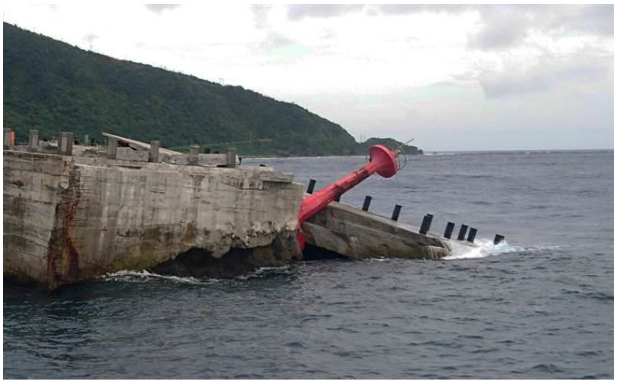
Due to population growth and impacts of climate change, severe sea states (e.g., typhoon-induced storm surges and storm waves) caused by extreme meteorological conditions such as typhoons, have been increasing the level of threat to human life and property in coastal zones worldwide [1]. Landfall caused by typhoons is considered a serious natural disaster [2,3,4]; however, major catastrophes led by huge storm waves usually occur when a typhoon approaches or passes coastal zones. In addition, storm waves not only damage harbors and seawalls but also infrastructure in coastal and nearshore regions [5,6]. For example, a roaring wave (wave height ≥ 12.0) destroyed a lighthouse in a fishing port in the southwestern waters of Taiwan when Typhoon Meranti (2016) was passing, without creating a landfall (Figure 1). Therefore, an assessment of storm wave hazards is urgently needed to provide useful information for decision-makers in order to reduce and mitigate disasters in coastal zones.

Similar to the storm surge hazard assessment conducted by the authors of [7,8,9] in the Caribbean and Yellow Sea, here, the goal of storm wave hazard assessment is to evaluate and better understand the natural attributes of storm waves (e.g., how high a storm wave is) in the nearshore waters of Taiwan. To achieve this aim, numerous hindcasts of storm waves should be carried out using a numerical model that can provide a high temporal and spatial resolution of marine meteorology. Numerical simulations of typhoon and wind storm-generated sea states have been continuously employed for research on severe hydrometeorology [10,11,12,13] because ocean surface waves that arise out of extreme weather conditions are of great interest to oceanographers and ocean engineers [13,14].

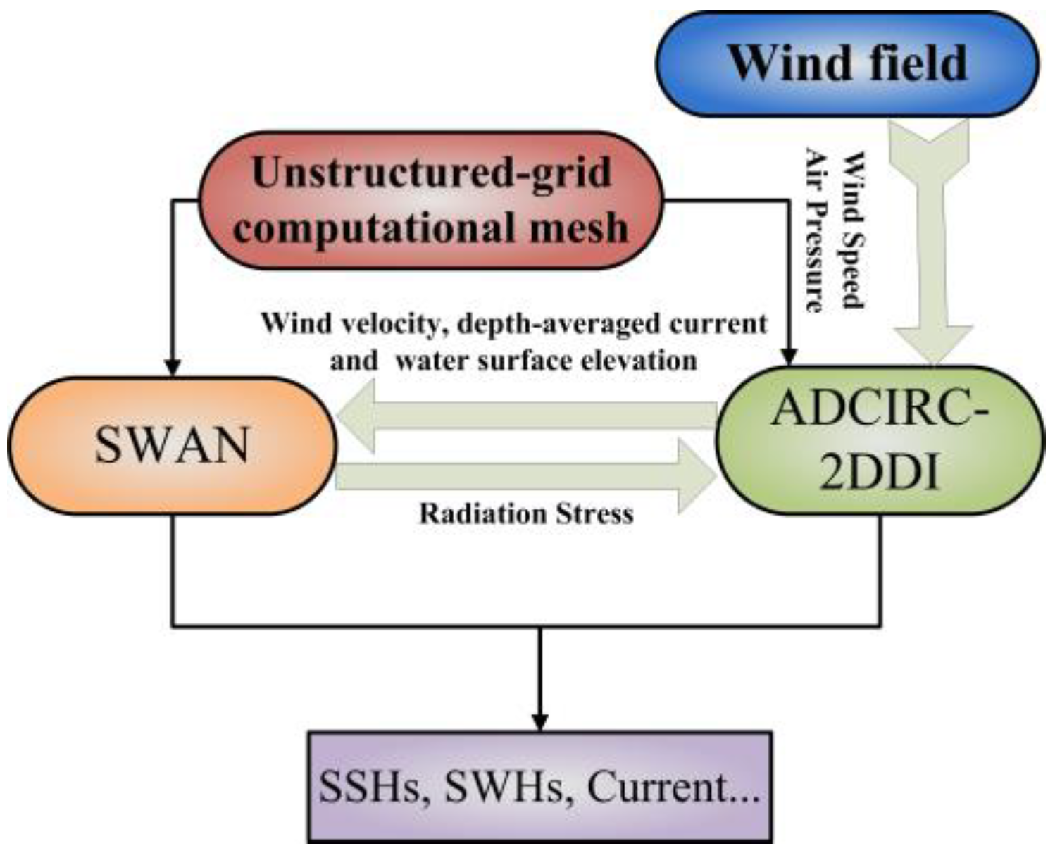
Although third-generation spectral wind wave models are able to predict wave heights (as long as the accurate wind field over the sea surface is provided [15]), wave–current interactions should not be excluded in storm wave hindcasting. Sun et al. [16] suggested that the wave–current interaction on surge elevation varied in space and time, and was more significant over the shelf than inside the inner bays. Additionally, the overall simulation accuracy of hurricane-induced waves is slightly improved if the wave–current interaction is considered. Refractions are triggered when waves propagate over spatially varying and strong currents [17,18]. Additionally, wave steepening can arise if the current direction is in contrast to the wave’s direction [19]. The effect that tide and surge have on the wave must also be considered in numerical models, since the incident wave height increases during rising tides in the coastal zone [20]. The effects of wave–tide and wave–current interactions on storm wave hindcasts are included in the present study by using a high-resolution, unstructured-grid and tide–surge–wave coupled modeling system. The system is composed of two models—a two-dimensional coastal hydrodynamic model and a third-generation spectral wave model—in the same computational domain. This scenario is able to minimize data interpolation errors. Many fully coupled models (e.g., SELFE-WWM-II, SCHISM-WWM-III) have been successfully applied to predict storm tides and storm waves [21] and identify the optimal offshore areas for deployment of wave energy converts in Taiwanese waters [22].

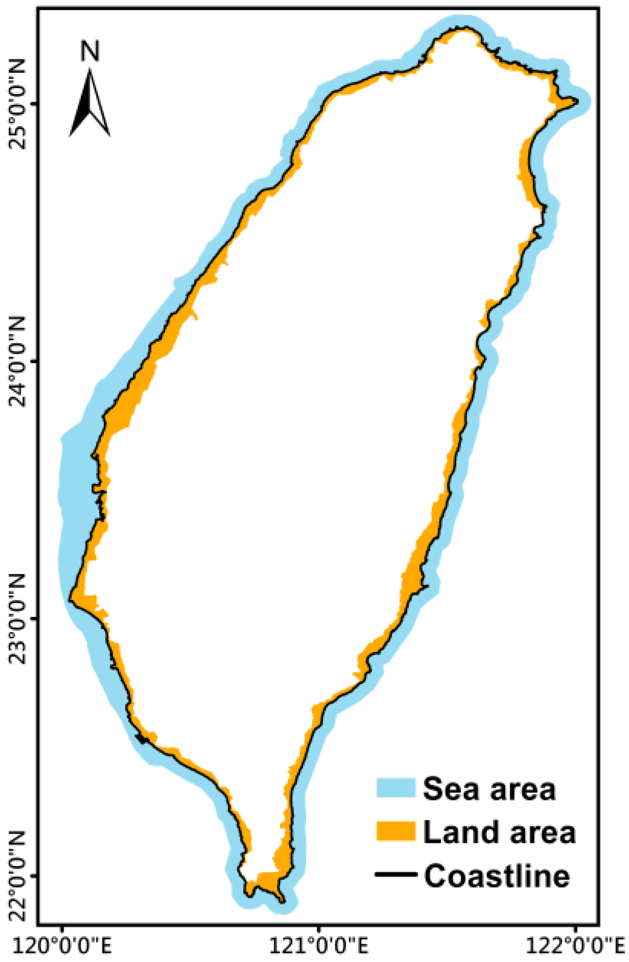
Many studies have focused on an analysis of storm surge hazards [7,8,9], but the potential impact of storm waves has received little attention. Shih et al. [23] reproduced waves induced by the highest intensity and lowest intensity typhoons selected from 1977 to 2016, and analyzed the possible wave threats along the coast of Taiwan. Although they generated the event-based maximum and minimum potential risk maps for typhoon-induced waves, their results only focused on the coastline. Here, the numerical investigation of storm wave hazards was conducted and applied to the sea areas of the coastal zone (SACZs) in Taiwan. The extent of the coastal zone is defined by the Ministry of the Interior in Taiwan. Figure 2 illustrates the coastal zone of Taiwan. The total of the land areas of the coastal zone (LACZ) is 3048.1 km², while the total SACZ covers 6117.5 km².

The present paper is organized as follows: a brief outline of the models is given, followed by the specification of boundary conditions. Then, in Section 2, the selection of typhoon events and the configuration of the models are given. Model validations for typhoon-induced storm waves employing three wind fields are described in Section 3. The results and discussions are shown in Section 4. The main conclusions are summarized in Section 5.

2. Materials and Methods

2.1. Two-Dimensional Hydrodynamic Model

ADCIRC (Advanced Circulation) is a continuous Galerkin finite element shallow-water model that solves for water levels and currents at a range of scales from rivers and tides to wind-driven storm surges. In addition, the resolution of the ADCIRC can vary from 20–30 km to 30–50 m [24,25,26,27]. Water levels are obtained through a solution of the Generalized Wave Continuity Equation (GWCE), and the currents are acquired via solving the vertically integrated momentum equations. A two-dimensional vertically integrated version of the ADCIRC (ADCIRC-2DDI) was utilized for simulating hydrodynamics in Taiwanese waters. The governing equations of the ADCIRC-2DDI in the Cartesian coordinate system are defined as follows:

$$\frac{\partial \zeta }{\partial t}+\frac{\partial \left(UH\right)}{\partial x}+\frac{\partial \left(VD\right)}{\partial y}=0$$

(1)

$$\frac{\partial U}{\partial t}+U\frac{\partial U}{\partial x}+V\frac{\partial U}{\partial y}=fV-g\frac{\partial }{\partial x}\left[\zeta +\frac{P_A}{{\rho }_0}-\alpha \hat{\psi }\right]+\frac{{\tau }_{sx}+{\tau }_{rx}-{\tau }_{bx}}{{\rho }_{0}H}+\frac{M_x+D_x}{H}$$

(2)

$$\frac{\partial V}{\partial t}+U\frac{\partial V}{\partial x}+V\frac{\partial V}{\partial y}=-fU-g\frac{\partial }{\partial y}\left[\zeta +\frac{P_A}{{\rho }_0}-\alpha \hat{\psi }\right]+\frac{{\tau }_{sx}+{\tau }_{rx}-{\tau }_{bx}}{{\rho }_{0}H}+\frac{M_y+D_y}{H}$$

(3)

where $\zeta (x,y,t)$ is the free surface elevation; $H=\zeta +h$ is the total water depth; $h$ is the bathymetric depth; $U(x,y,t)$ and $V(x,y,t)$ are the vertical integrated velocity components in the x- and y-directions, respectively; $f$ is the Coriolis factor; $g$ is the acceleration due to gravity; ${\rho }_0$ is the reference density of water; $\hat{\psi }$ is the Newtonian equilibrium tidal potential; $\alpha$ is the effective earth elasticity factor; $P_A(x,y,t)$ is the atmospheric pressure at the free surface; M refers to lateral stress gradients; and D refers to the momentum dispersion terms. ${\tau }_{sx}$ and ${\tau }_{sy}$ are the wind stress components in the x and y-directions, respectively, and can be expressed as follows:

$$\begin{gathered} {\tau }_{sx}={\rho }_a{C}_s\sqrt{W_x{}^2+W_y{}^2}{W}_x \\ {\tau }_{sy}={\rho }_a{C}_s\sqrt{W_x{}^2+W_y{}^2}{W}_y \end{gathered}$$

(4)

where C_s is the wind drag coefficient; ${\rho }_a$ is the air density; and W_x and W_y are the wind velocity components at a 10-m height above the sea surface in the x- and y-directions, respectively. C_s should be limited at high wind speeds [28]; thus the formula of C_s in the ADCIRC-2DDI is given as:

$$C_s=\{\begin{array}{c}0.001\times \left(0.75+0.067\times W\right),\mathrm{if}{C}_s\le 0.003\\ 0.003,\mathrm{if}{C}_s>0.003\end{array}$$

(5)

where $W$ is the resultant wind speed.

The following formulas are used to calculate the bottom shear stress components in the x- and y-directions:

$$\begin{gathered} {\tau }_{bx}={\rho }_0{C}_d\sqrt{U^2+V^2}V \\ {\tau }_{by}={\rho }_0{C}_d\sqrt{U^2+V^2}V \end{gathered}$$

(6)

A Manning’s n formulation is adopted for computing the hydraulic friction C_d in the ADCIRC-2DDI:

$$C_d=g{n}^2/H^{1/3}$$

(7)

Based on the type of sea-bottom material, the Manning coefficient n of 0.025 was set in the mode, and therefore C_d varies with H according to Equation (7).

According to [29], the radiation stress tensor components can be represented as:

$$\begin{gathered} S_{xy}={\displaystyle \underset{0}{\overset{2\pi }{\int }}{\displaystyle \underset{0}{\overset{\infty }{\int }}N\sigma \frac{C_g}{C_p}}}\sin \left(\theta \right)\cos \left(\theta \right)d\theta d\sigma \\ {S}_{xx}={\displaystyle \underset{0}{\overset{2\pi }{\int }}{\displaystyle \underset{0}{\overset{\infty }{\int }}N\sigma \left[\frac{C_g}{C_p}\left({\cos }^2\left(\theta \right)+1\right)-\frac{1}{2}\right]}}d\theta d\sigma \\ {S}_{yy}={\displaystyle \underset{0}{\overset{2\pi }{\int }}{\displaystyle \underset{0}{\overset{\infty }{\int }}N\sigma \left[\frac{C_g}{C_p}\left({\sin }^2\left(\theta \right)+1\right)-\frac{1}{2}\right]}}d\theta d\sigma \end{gathered}$$

(8)

where N is the wave action, $\sigma$ is the relative angular frequency of waves, $\theta$ is the wave direction, and C_g and C_p are the wave group velocity and wave phase velocity, respectively. The wave-induced stress, ${\tau }_{rx}$ and ${\tau }_{ry}$, were therefore obtained via the approaches presented by Longuet-Higgins and Stewart [30,31]:

$$\begin{gathered} {\tau }_{rx}=-\frac{\partial S_{xx}}{\partial x}-\frac{\partial S_{xy}}{\partial y} \\ {\tau }_{ry}=-\frac{\partial S_{xy}}{\partial x}-\frac{\partial S_{yy}}{\partial y} \end{gathered}$$

(9)

2.2. Third-Generation Spectral Wave Model

A state-of-the-art third-generation spectral wind wave model, an unstructured-grid SWAN (Simulating WAves Nearshore, [31]), was adopted to reproduce the significant wave heights (SWHs) caused by historical typhoon events in the nearshore waters of Taiwan. SWAN computes random short-crested wind-generated waves in coastal regions and inland waters. The theoretical and numerical backgrounds for SWAN were described in [32,33,34,35]. The spectral action balance equation of SWAN is given as follows:

$$\frac{\partial N}{\partial t}+\frac{\partial \left(C_{gx}+\mathrm{U}\right)N}{\partial x}+\frac{\partial \left(C_{gy}+\mathrm{V}\right)N}{\partial y}+\frac{\partial \left(C_{\sigma }N\right)}{\partial \sigma }+\frac{\partial \left(C_{\theta }N\right)}{\partial \theta }=\frac{S_{tot}}{\sigma }$$

(10)

where C_gx and C_gy are the wave group velocity components in the x- and y-directions, respectively; and $C_{\sigma }$ and $C_{\theta }$ are the propagation velocities in $\sigma ,\theta$ space. The sum of the source terms S_tot represents wave growth by wind. The 36 directional bins of constant width 10° and 40 frequency bins that increase logarithmically over the range 0.031–1.42 Hz were utilized in SWAN. Wave-breaking values in shallow-water areas are estimated following [36] with a breaking index of 0.73.

The ADCIRC-2DDI passes wind velocities, water surface elevations, and depth-averaged currents to SWAN. SWAN then computes the radiation stress gradients and transfers them to ADCIRC-2DDI. Figure 3 exhibits the coupling processes of the ADCIRC+SWAN modeling system. More details can be found in [37].

2.3. Model Setup

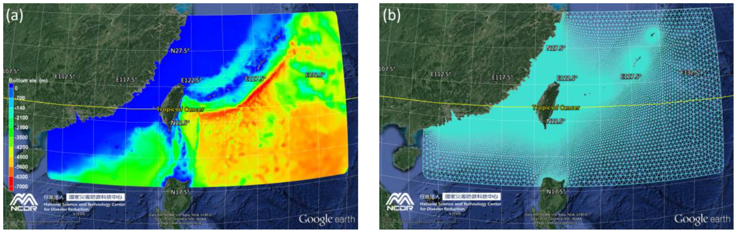
The computational domain involves the entirety of Taiwan and its main offshore islands, which extend from 111° E to 135° E and 18° N to 30° N (as shown in Figure 4a). The computational domain has been found to be sufficiently wide for simulating the sea states induced by typhoons that are traveling long distances from the east to the west of Taiwan.

The gridded bathymetry data utilized in this study was composed of a global and a local dataset. The global dataset was obtained from the General Bathymetric Chart of the Oceans (GEBCO) with a resolution of 30 arc-seconds. GEBCO was generated by combining quality-controlled ship depth soundings with interpolations between sounding points guided by satellite-derived gravitational data. The local dataset was provided by the Department of Land Administration and the Ministry of the Interior in Taiwan, with a resolution of 200 m. This dataset only covers the longitudes of 100° E to 128° E and the latitudes of 4° N to 29° N. Thus, the bathymetries of the computational domain were interpolated from a combination of the GEBCO and local datasets (Figure 4a). The model meshes were constructed using 318,449 triangular cells and 163,957 non-overlapping unstructured grids. Mesh resolution varies from 40 km at open ocean boundaries to 200 m along the coastline of Taiwan and its small offshore islands (Figure 4b).

A time step of 1 s was chosen for the ADCIRC-2DDI to achieve stability of the model. SWAN is unconditionally stable, and therefore its time step can be relatively large. The present hindcasts utilize a time step of 600 s for SWAN and the coupling interval is taken to be the same as the time step of SWAN (i.e., the ADCIRC-2DDI and SWAN exchange information every 10 min).

2.4. Model Forcing

Tidal forcing was used to drive the model with imposing tidal levels along the open boundaries of the computational domain. The harmonic constants of eight tidal constituents (M₂, S₂, N₂, K₂, K₁, O₁, P₁, and Q₁) that were extracted from a regional inverse tidal model (China Seas & Indonesia 2016 [38]), were employed to generate the tidal levels at each time step. Despite the open boundaries of the SWAN model being placed far away from the area of interest, the wave boundary conditions were prescribed by a regional WaveWatch III (WW III) model implemented by National Science and Technology Center for Disaster Reduction (NCDR) of Taiwan with a spatial resolution of 0.5° and a temporal resolution of 1 h. The regional WW III model covers the area of longitude from 100° E to 150° E and latitude from 10° N to 40° N (not shown).

An accurate wind forcing is crucial for the improvement of wind wave modeling [39], although the wind field specification for typhoons is not a straightforward task [40]. The ADCIRC+SWAN was driven by a wind speed at 10 m above sea level. In the present study, three kinds of wind field were adopted in order to obtain the acceptable SWH hindcasts:

(1) Parametric typhoon model

Using an analytical parametric model is a common way to construct the wind and air pressure fields of typhoons. Many parametric typhoon models have been developed to provide meteorological information for storm surge or storm wave modeling [41,42,43,44,45,46]. Since the authors of [47] found that the analytical models provided very similar results, the parametric typhoon model proposed in [43] was employed:

$$P_A=P_c+\left(P_n-P_c\right)\exp [{(\frac{R_{\max }}{r})}^B]$$

(11)

$$W_g=\sqrt{\frac{B\left(P_n-P_c\right)}{{\rho }_a}{\left(\frac{R_{\max }}{r}\right)}^B\exp {\left(-\frac{R_{\max }}{r}\right)}^B+{\left(\frac{rf}{2}\right)}^2}-\left(\frac{rf}{2}\right)$$

(12)

where W_g is the gradient wind; P_A is the air pressure at arbitrary point; P_n is the ambient pressure; P_c is the typhoon central air pressure; R_max is the radius to the maximum wind speed; r is the radial distance from the typhoon’s center to an arbitrary point; W_H is the wind speed; ${\rho }_a$ is the air density; f is the Coriolis factor; and B is a characterized parameter presented by [48]. The wind field was modified from gradient height to 10 m above sea surface with a wind-reducing coefficient of 0.85 following [49]. With regard to R_max, the formula adopted to simulate storm surges in the northwest Pacific Ocean was used [50]:

$$\ln \left(R_{\max }\right)=c_0+c_1\Delta P+\epsilon$$

(13)

where $\Delta P=P_n-P_c$; $c_0$, $c_1$ and $\epsilon$ were set to be 5.0377, −0.0232 and 0.4502, respectively.

A highly asymmetric structure in a typhoon often leads to large errors in storm surge and wind wave forecasting; however, the asymmetric structure of a typhoon cannot be represented by the original Holland model. Georgiou [51] introduced a translation speed (W_t) to overcome this restriction, so then the parametric typhoon wind (W_PT) becomes:

$$W_{PT}=W_g+W_t\times 0.5\sin \left(\vartheta \right)$$

(14)

where $\vartheta$ is the angle from the direction of the typhoon movement.

(2) Reanalysis typhoon wind data

Reanalysis typhoon wind fields (W_RT) produced by the ERA-Interim were acquired from the European Center for Medium-Range Weather Forecasts (ECMWF) public datasets. ERA-Interim is the latest global atmospheric reanalysis dataset and is normally updated once per month with a delay of two months [52]. The 10-m U and V wind components were extracted from ERA-Interim reanalysis data at a temporal resolution of 6 h (four analysis fields per day, at 00:00, 06:00, 12:00 and 18:00 Coordinated Universal Time(UTC)) and a spatial resolution of 0.125° × 0.125°. W_RT was converted to each unstructured grid of the ADCIRC+SWAN using the Inverse Distance Weighting (IDW) method.

(3) Hybrid typhoon model

The parametric typhoon model generally produces high accurate wind fields near the center of the typhoon; however, the accuracies decrease as the distance from the typhoon center increases. In contrast, reanalysis wind data is inferior around the typhoon center but superior in the areas away from the center of the typhoon [53]. A combined usage of the parametric typhoon model and a reanalysis wind data is believed to generate better wind fields for an entire typhoon. The superposition method proposed by [54] was employed to create typhoon wind fields. The formulas for the calculation of the hybrid typhoon wind field (W_HT) are as follows:

$$W_{HT}=\{\begin{array}{cc}{W}_{PT}\hfill & \hfill r<R_1\\ \left(1-\alpha \right)W_{PT}+\alpha W_{RT}\hfill & \hfill R_1\le r\le R_2\\ W_{RT}\hfill & \hfill r>R_2\end{array}$$

(15)

where $\alpha =\left(r-R_1\right)/\left(R_2-R_1\right)$; R₁ and R₂ are two boundary limits in the transition zone and were set as 8R_max and 10R_max, respectively, based on the results of surge-wave coupled simulations in the typhoon-prone coastal areas of China [55].

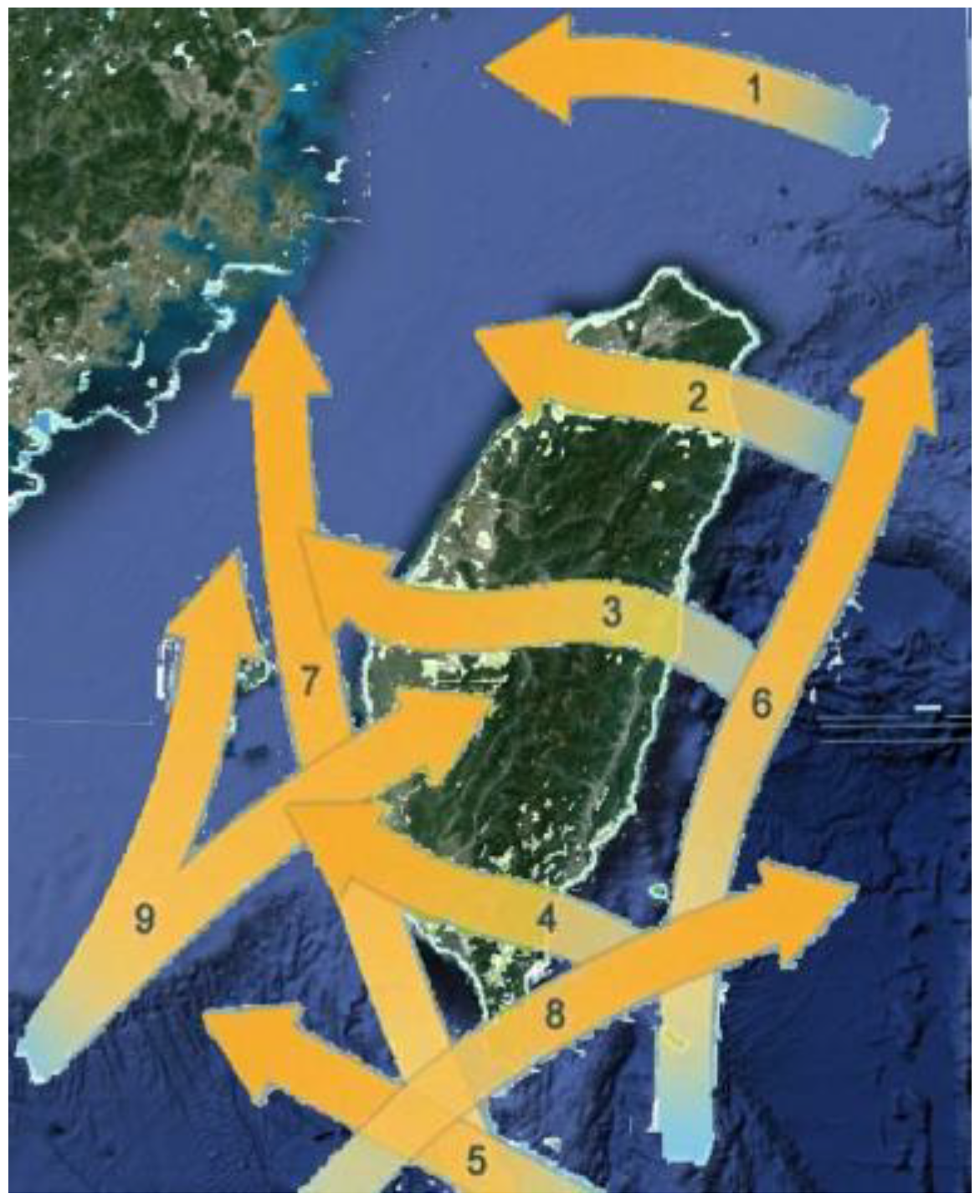
2.5. Typhoon Events

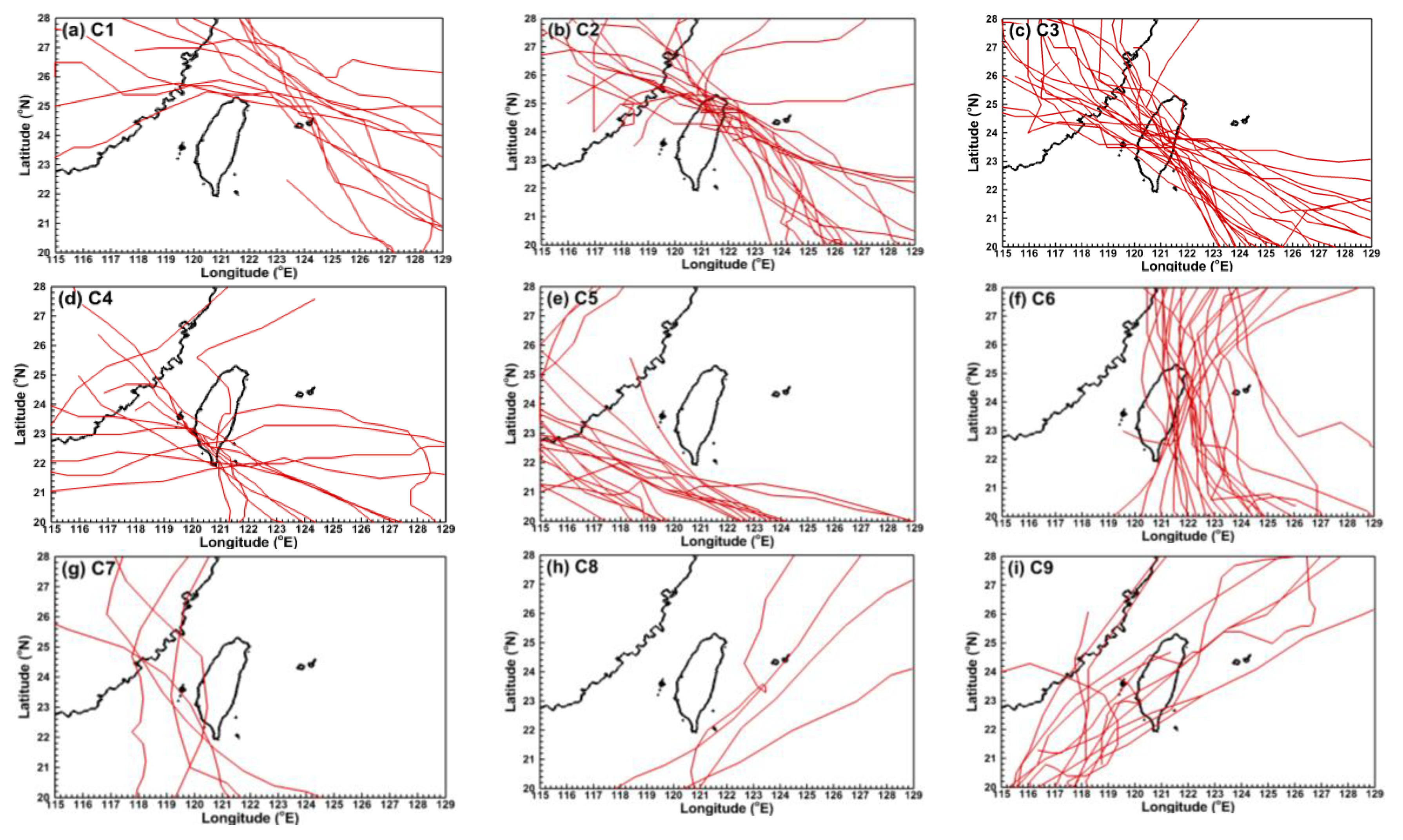
According to a typhoon’s track, the Central Weather Bureau (CWB) of Taiwan classifies typhoon events into nine categories (hereinafter referred to as C1 through C9, as shown in Figure 5). For example, a typhoon is classified as C1 if its track passed the northern waters of Taiwan and moved to the west or the northwest. A total of 124 typhoon events that impacted Taiwan were selected (the event would be selected if land or sea warnings about a typhoon were issued from the CWB) from the past 40 years (1978 to 2017). The hindcasting SWHs of these 124 typhoons were used to create storm wave hazard maps of each category for the SACZs. Nine storm wave hazard maps were finally employed to generate a comprehensive storm wave hazard map for the SACZs of Taiwan. Figure 6a–i demonstrates the tracks of typhoons for C1 to C9. The corresponding occurrences of typhoons are listed in

Table 1. Number of typhoon events corresponding to each category during the period 1978–2017.

Count	Category
	C1	C2	C3	C4	C5	C6	C7	C8	C9
Typhoon number	12	15	23	12	17	21	5	4	13

.

2.6. Metrics for Evaluation of Model Performance

Mean absolute error (MAE), root-mean-square error (RMSE), mean absolute percentage error (MAPE), and skill were used as criteria to evaluate the model performance for hindcasts of SWHs. It must be noted that the MAPE can only be used when there are no zero values among observations. A skill value of 1 means a perfect performance. A skill value ranging between 0.65 and 1.0 indicates excellent performance. A very good performance is in the range of 0.5 to 0.65; a good performance is in the range of 0.2 to 0.5, and a skill value less than 0.2 represents a poor performance [56]. The formulas for MAE, RMSE, MAPE, and skill are given as:

$$\mathrm{MAE}=\frac{1}{m}{\displaystyle \sum _{i=1}^m\left|{\mathrm{O}}_i^o-{\mathrm{O}}_i^h\right|}$$

(16)

$$\mathrm{RMSE}=\sqrt{\frac{{\displaystyle \sum _{i=1}^m{\left({\mathrm{O}}_i^o-{\mathrm{O}}_i^h\right)}^2}}{m}}$$

(17)

$$MAPE=\frac{1}{N}{\displaystyle \sum _{i=1}^N\left|\frac{{\mathrm{O}}_i^o-{\mathrm{O}}_i^h}{{\mathrm{O}}_i^o}\right|}\times 100$$

(18)

$$skill=1-\frac{{\displaystyle \sum _{i=1}^m{\left|{\mathrm{O}}_i^h-{\mathrm{O}}_i^o\right|}^2}}{{\displaystyle \sum _{i=1}^m{\left(\left|{\mathrm{O}}_i^h-\overline{\mathrm{O}}{}^o\right|+\left|{\mathrm{O}}_i^o-\overline{\mathrm{O}}{}^o\right|\right)}^2}}$$

(19)

where m is the total number of data points, ${\mathrm{O}}_i^h$ is the hindcast, ${\mathrm{O}}_i^o$ is the observation, and ${\overline{\mathrm{O}}}^o$ is the mean value of the observations.

3. Model Performance Using Different Wind Fields

ADCIRC+SWAN has been used and validated for various typhoon events all over the world [38,57,58,59,60]. It has been found to give good performances for hindcasting the hydrodynamics and sea states around islands [7,8]. For the purpose of accurately hindcasting typhoon-driven SWHs, two validation tests were conducted using three kinds of wind fields. Additionally, only SWHs were compared since the main aim of the present study is to assess the hazard levels of storm waves.

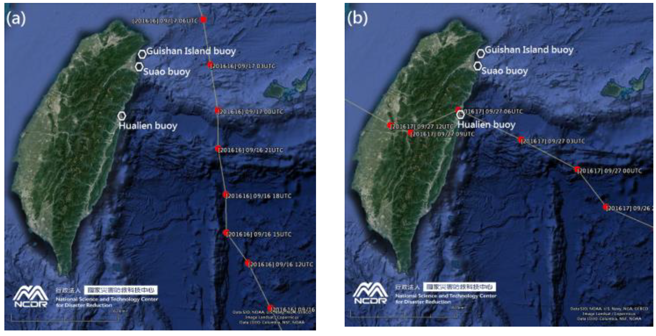
The SWHs measurements recorded at three buoys by the CWB in 2016 were adopted to validate the ADCIRC+SWAN. The tracks of Typhoon Malakas (2016) and Typhoon Megi (2016), and the locations of the wave buoys are shown in Figure 7 (Figure 7a for Malakas and Figure 7b for Megi). The Guishan Island, Suao, and Hualien buoys are situated along the northeastern to eastern nearshore waters of Taiwan. The historical typhoon data were obtained from the Regional Specialized Meteorological Center (RSMC) Tokyo-Typhoon Center. The RSMC provides information on typhoons in the western North Pacific and the South China Sea, including present and forecasted positions, as well as on the movement and intensity of typhoons.

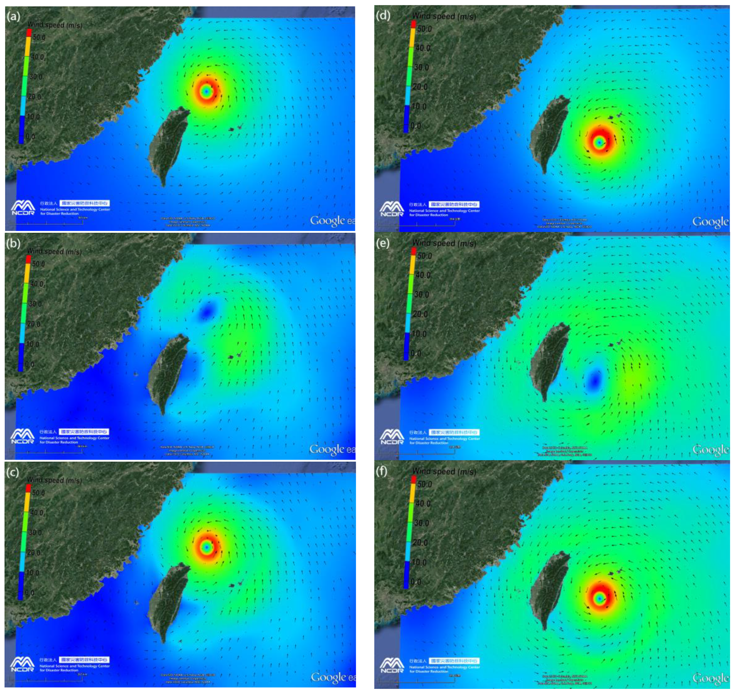
Figure 8a–c depicts the wind field snapshots of the ADCIRC+SWAN for Typhoon Malakas (2016) exerted by parametric (Figure 8a), reanalysis (Figure 8b), and hybrid (Figure 8c) typhoon models. As mentioned in Section 2.4, the parametric typhoon model generates higher and more accurate wind fields near the center of a typhoon (Figure 8a) but has poor quality in reproducing wind fields further away from the typhoon’s center. The performance of reanalysis typhoon wind data is contrary to the parametric typhoon model (Figure 8c). It is quite obvious that a combination of the wind fields from these two models (hybrid typhoon model, Figure 8b) would create an advantage for the SWH hindcasts. Similar results for Typhoon Megi (2016) are found in Figure 8d–f.

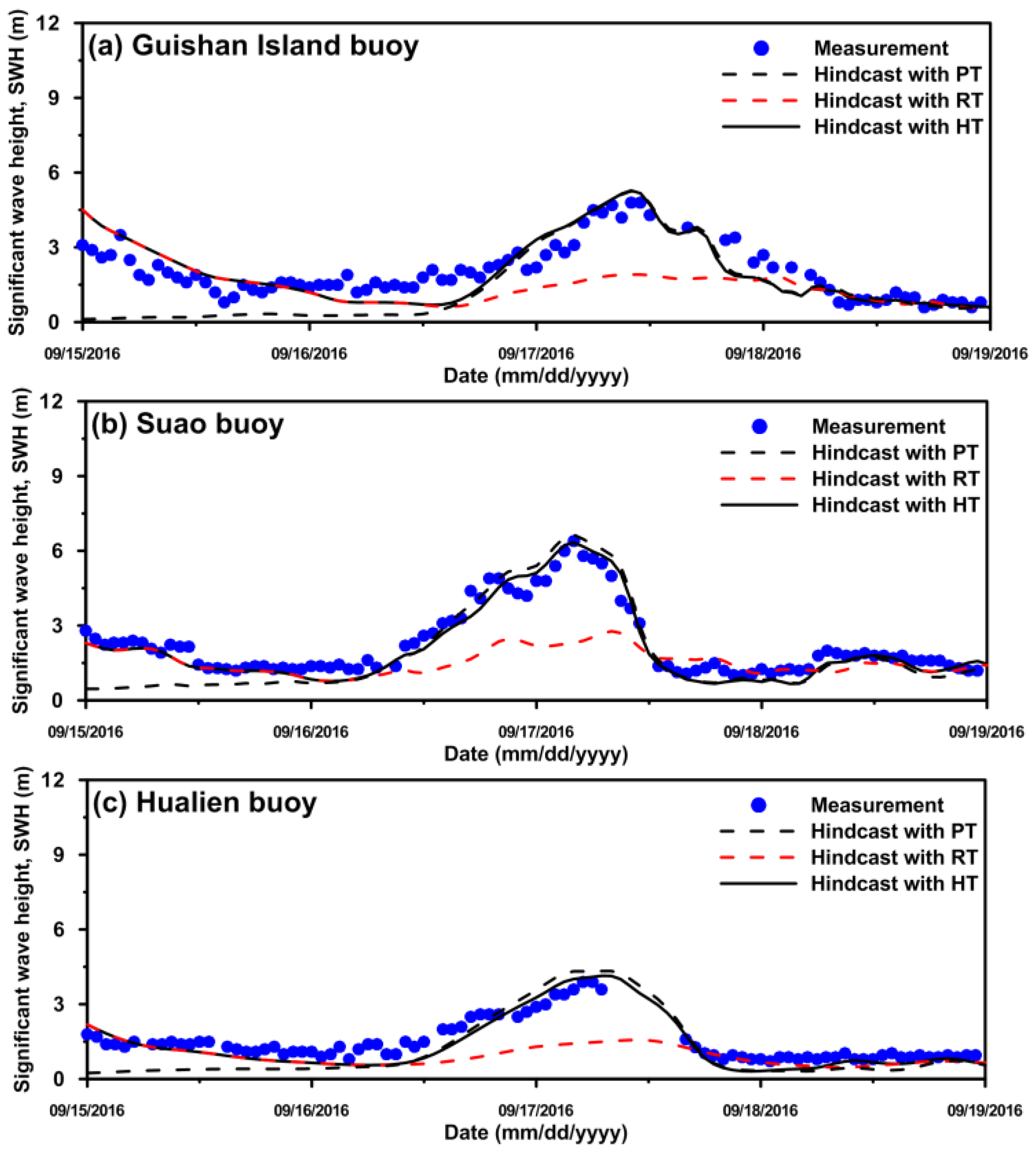
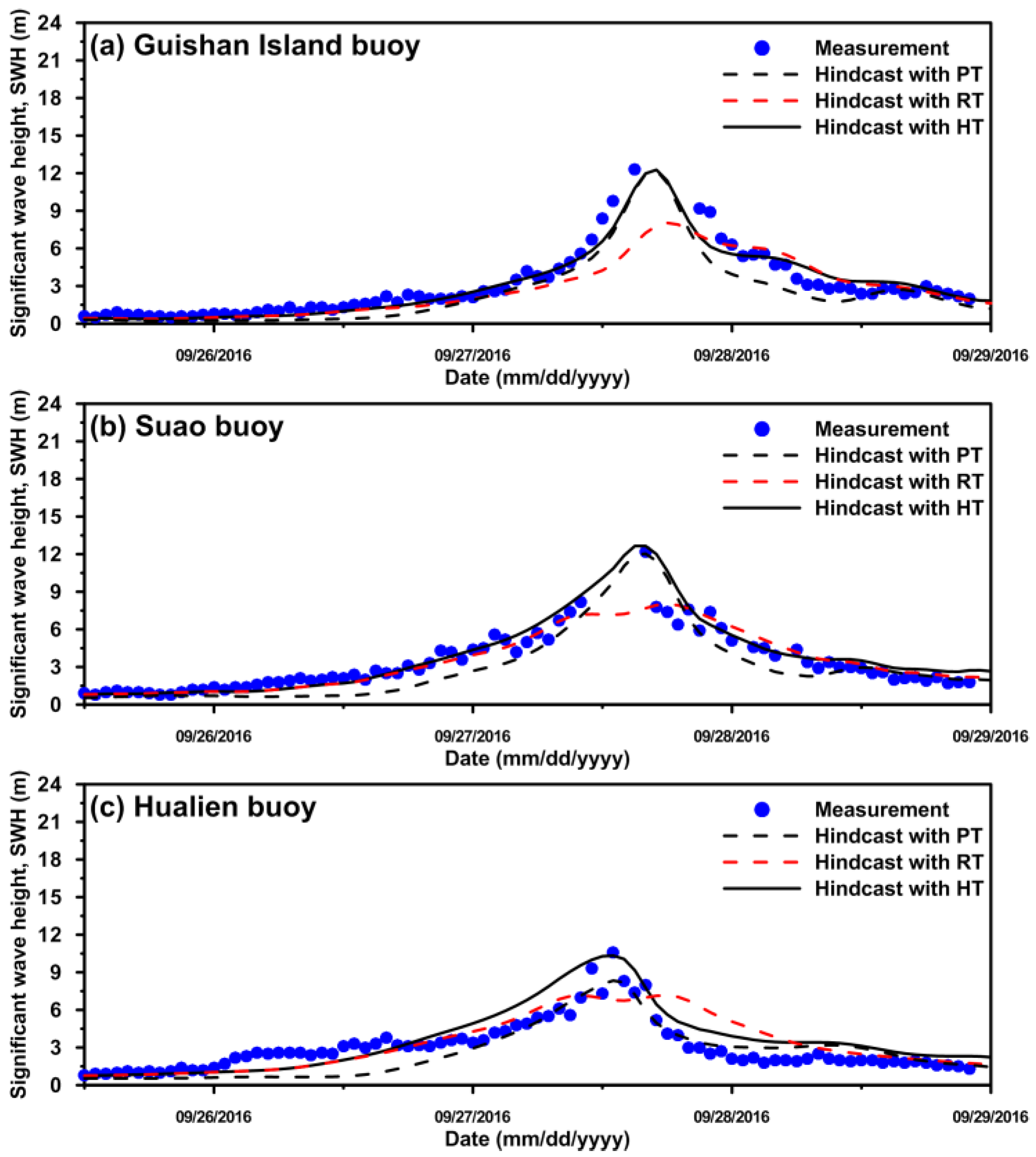
The model–data comparisons of the SWHs caused by Typhoon Malakas from 15 September 2016 to 18 September 2016 are presented in Figure 9 (Figure 9a for the Guishan Island, Figure 9b for the Suao, and Figure 9c for the Hualien buoys). It can be seen from Figure 9a–c that the maximum SWH was approximately 6.0 m at the Guishan Island and Suao buoys and was only 4.0 m at the Hualien buoy due to Typhoon Malakas just passing through the eastern waters of Taiwan without creating landfall (Figure 7a). Figure 10a–c show the SWHs comparison between measurements and hindcasts for Typhoon Megi from 26 September 2016 to 29 September 2016. The maximum SWH exceeded 12.0 and 10.0 m at the Guishan Island (Figure 10a), Suao (Figure 10b) and Hualien (Figure 10c) buoys because Typhoon Megi crossed Taiwan from east to west and made landfall in Hualien County (Figure 7b). Using the parametric (black dashed line in Figure 9 and Figure 10) and hybrid typhoon (black solid line in Figure 9 and Figure 10) models could reproduce the similar peak for SWHs; however, the SWHs were underestimated, except for peaks, when the parametric typhoon wind fields were exerted on the ADCIRC+SWAN. The performance of the SWH hindcasts by adopting reanalysis typhoon wind data (the red solid line in Figure 9 and Figure 10) is contrary to the parametric typhoon model. In general, the SWHs generated by the hybrid typhoon model were in greater agreement about observations in the peak and normal phases.

The statistical errors of the differences between the hindcasts and the observations for the three wave buoys using different typhoon wind fields were calculated and are listed in

Table 2. Statistical errors of the model–data difference for significant wave height (SWH).

Station	Wind Field	MAE (m)	RMSE (m)	MAPE (%)	Skill
Guishan Island	PT	0.93	1.19	46.04	0.86
	RT	0.82	1.21	32.87	0.96
	HT	0.53	0.71	25.68	0.95
Suao	PT	0.78	0.96	32.98	0.98
	RT	0.66	1.02	22.53	0.97
	HT	0.41	0.49	17.99	0.98
Hualien	PT	0.81	0.95	4459	0.89
	RT	0.84	1.16	37.69	0.71
	HT	0.66	0.75	29.77	0.94

Note: PT: Parametric typhoon model; RT: Reanalysis typhoon wind data; HT: Hybrid typhoon model; MAE: Mean absolute error (m); RMSE: Root-mean-square error (m); MAPE: mean absolute percentage error (%).

. The minimal MAE, RMSE and MAPE are 0.41 m, 0.49 m and 17.99%, and the highest skill is found to be 0.98 for the Suao buoy when adopting the hybrid typhoon model. Slight discrepancies still occurred, even with good agreement between hindcasted and measured SWHs. This phenomenon may be due to the lower spatial and temporal resolutions of the typhoon wind field data from reanalysis.

The improvements in the hindcasting of SWHs are significant by means of a model–data comparison using three typhoon wind forcings. Typhoon-induced SWHs reproduced by the ADCIRC+SWAN fully coupled model adopting hybrid wind fields are deemed very reliable and can be further utilized for assessing storm wave hazards in the nearshore waters of Taiwan.

4. Results and Discussion

The typhoon-driven SWHs were reproduced by hindcasting the historical events of each category in the waters surrounding Taiwan from 1978 to 2017. In total 124 typhoon events were selected from the database of the CWB for SWH hindcasting. The tracks of the typhoon and the number of typhoon events for each category are shown in Figure 6 and Table 1. The most frequent typhoon category is C3, with 23 occurrences, while the least frequent is C8, with only 4 occurrences.

4.1. Producing Storm Wave Hazard Maps for Each Typhoon Category

The maximum hindcasting SWHs of each typhoon event were extracted, and then the maximum SWHs among typhoon events of the same category were extracted again. Finally, the maximum SWHs of each category were classified into five hazard levels (I to V) and created the storm wave hazard map for the nearshore waters of Taiwan (i.e., the SACZs). The hazard is regarded as a level I when the SWH less than 3.0 m; SWHs lying between 3.0 and 6.0 m are considered hazard level II; the hazard is level III when the SWH ranges from 6.0 to 9.0 m; SWHs of 9.0–12.0 m are considered hazard level IV; and SWHs larger than 12.0 m are deemed hazard level V. The classification of hazard levels and SWHs and their corresponding descriptions are listed in

Table 3. The classification of hazard levels corresponding to the ranges of significant wave heights (SWHs).

Hazard Level	Range of SWHs (m)	Descriptions
I	<3.0	Small Wave
II	(3.0–6.0)	Big Wave
III	(6.0–9.0)	Giant Wave
IV	(9.0–12.0)	Violent Wave
V	≥12.0	Roaring Wave

Note: the range of SWHs was given by the Central Weather Bureau of Taiwan and modified by the present study.

.

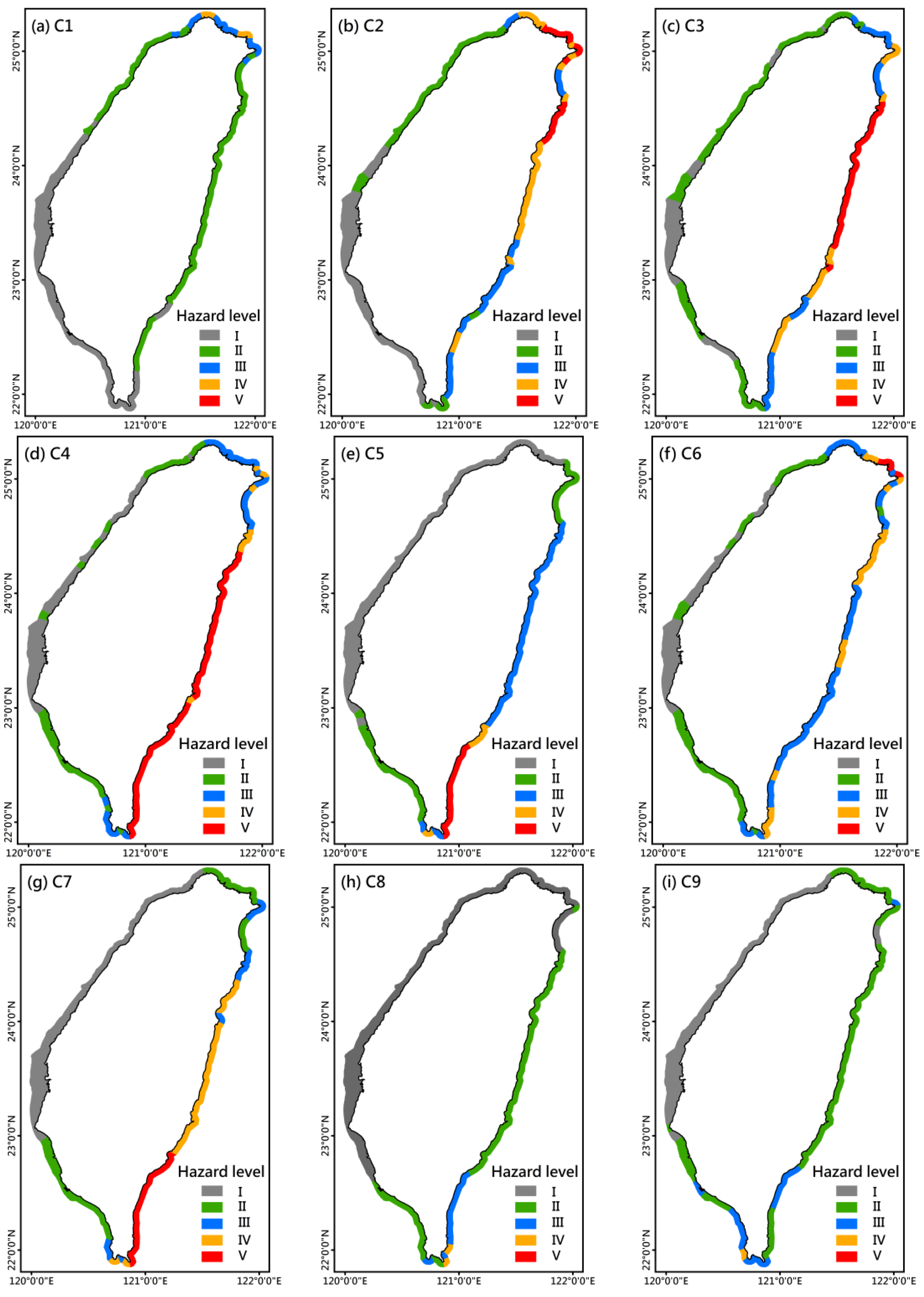
Figure 11a–i illustrate the storm wave hazard maps of C1 to C9 for the SACZs. The black solid line is the coastline of Taiwan; gray, green, blue, yellow and red represent hazard level I, hazard level II, hazard level III, hazard level IV, and hazard level V, respectively. As shown in Figure 11a, the storm waves of C1 only significantly impact part of the northern SACZs of Taiwan and lie at hazard level III and IV; the rest of the SACZs are below hazard level II. The storm waves of the C2 influence most of the northern and northeastern SACZs, and part of the eastern SACZs. The northern and northeastern SACZs are threatened by hazard level III, hazard level IV and hazard level V, whereas the eastern SACZs are threatened by hazard level III and hazard level IV (Figure 11b). The extents of hazard level IV and hazard level V of C3 are shifted to the southern and northern part of the eastern SACZs; the lower part of the eastern SACZs is almost exclusively influenced by hazard level III (Figure 11c). The areas threatened by hazard level V are extended to the entire eastern SACZs, and the largest area of the SACZ belonging to hazard level V is found in C4. Hazard levels III and IV are distributed over the northeastern SACZs. The lower part of the southwestern and the southernmost SACZs are occupied by hazard level III (Figure 11d).

Figure 11e depicts the distribution of the hazard levels of C5 for the SACZs. The southern and northern parts of the eastern SACZs are almost entirely influenced by hazard level III to hazard level V, except for the northeastern and southwestern SACZs, which are affected by hazard level II. For the storm wave of C6, hazard levels III and IV threaten the entire northernmost, northeastern, and eastern, as well as the southernmost SACZs. However, hazard level V appears in a fraction of the northern SACZs (Figure 11f). It is very similar to C5 in that the hazard level V of C7 is distributed in the southeastern SACZs. The eastern SACZs remain in hazard level IV, while hazard levels II and III impact the northwestern and southwestern SACZs (Figure 11g). Regarding the storm wave maps of C8 and C9 (Figure 11h,i), hazard level V is absent. Hazard levels III and IV are restricted to the southeastern and southern SACZs. The remaining SACZs belong to hazard levels I and II.

The area of the SACZs corresponding to each hazard level and typhoon category are calculated and summarized in

Table 4. The areas of the SACZs corresponding to each hazard level and typhoon category.

Hazard Level	Category
	C1	C2	C3	C4	C5	C6	C7	C8	C9
I	2906.5	2183.0	1402.2	1898.9	2847.2	1714.9	2477.5	3513.6	2508.7
II	2564.2	1309.7	2179.1	1307.0	1168.2	1546.3	1331.3	2020.7	2793.0
III	490.5	1012.5	941.8	926.4	1364.4	1805.7	533.8	489.0	761.4
IV	156.2	1041.2	668.7	287.2	210.0	904.5	1092.8	94.3	54.3
V	0.0	571.0	925.7	1698.0	527.7	146.0	682.1	0.0	0.0

Unit: km².

. The largest area of the SACZs for hazard level I was found to be 3513.6 km² in C8. Hazard level II occupies the area of the SACZs, with its largest area being 2793.0 km² for C9. Hazard level III and IV have the largest areas of the SACZs of 1805.7 and 1092.8 km² for C6 and C7, respectively. Additionally, C4 is associated with the largest area of the SACZs at 1698.0 km² for hazard level V.

4.2. Assessing the Comprehensive Storm Wave Hazard

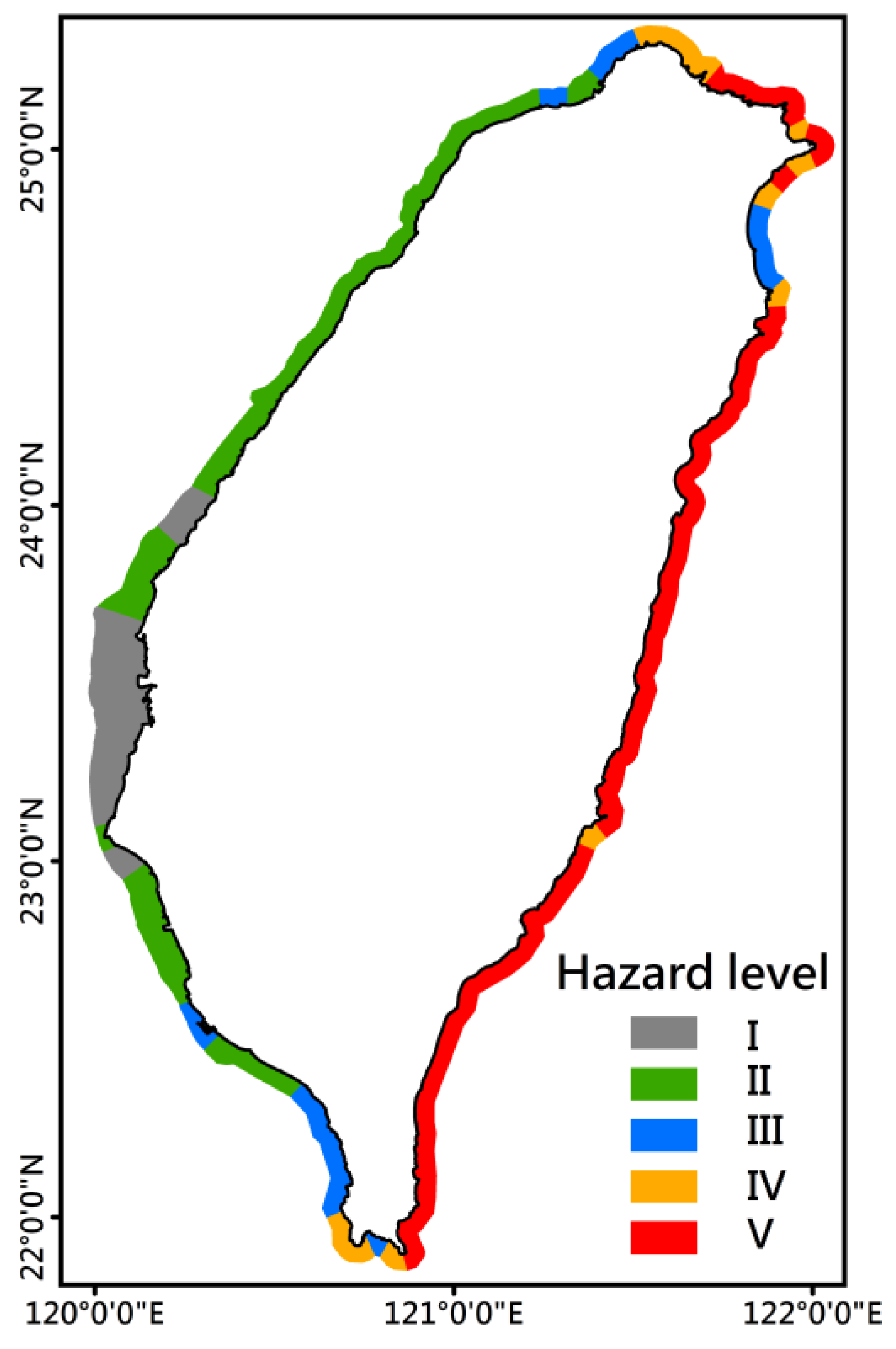
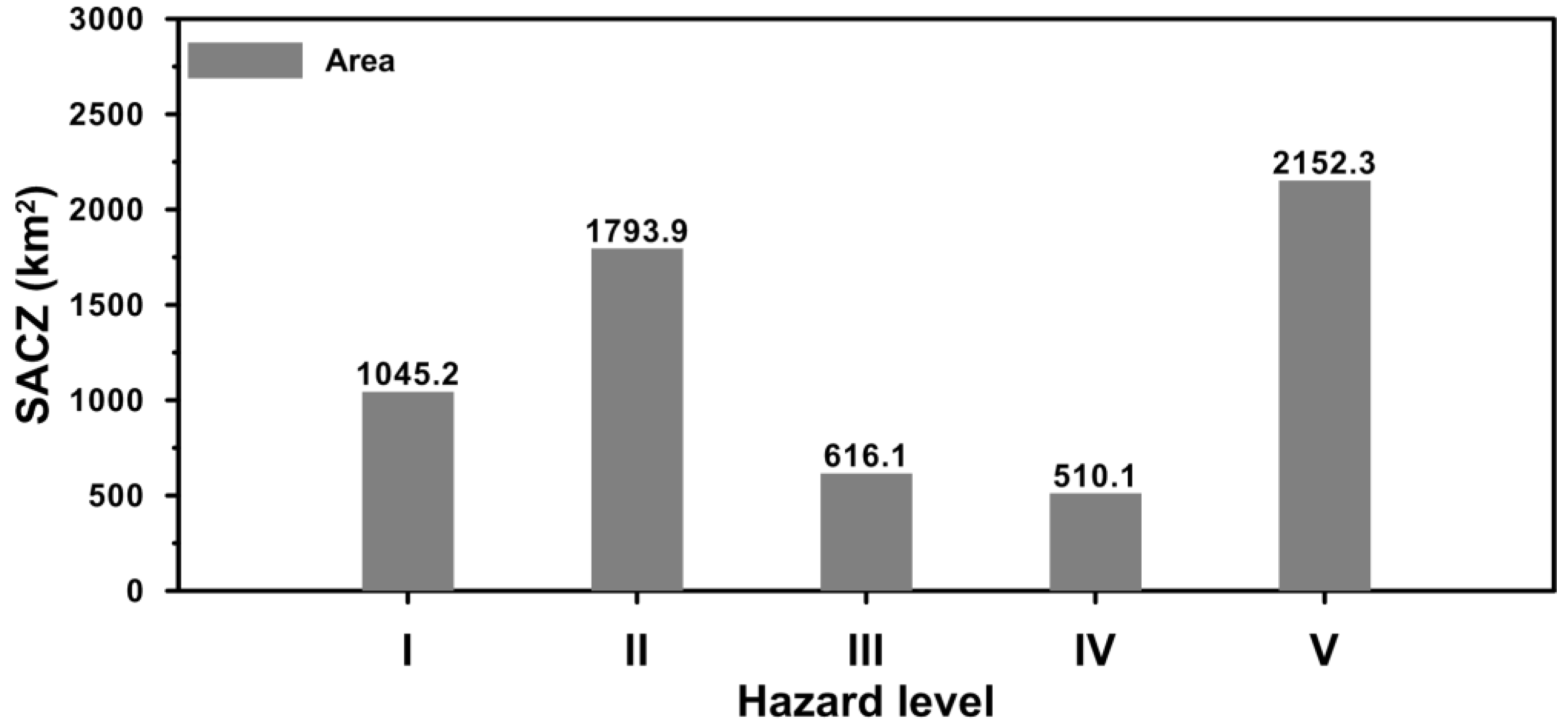
The same approach for producing storm wave hazard maps of each typhoon category was adopted to assess the comprehensive storm wave hazard in the SACZs of Taiwan. The maximum SWHs among nine categories were extracted and classified into five hazard levels (I to V). A comprehensive storm wave hazard map of the nine categories mapped by the present study is shown in Figure 12. In general, except for a portion of the northeast (impacted by hazard III), the northern and a complete eastern SACZs of Taiwan are potentially threatened by severe sea states (hazard IV and V) when typhoons are present. The southwestern SACZs are generally affected by hazard III, while the western SACZs are primarily subjected to the mild effects (hazard I and II) of typhoon-driven storm waves. This is because the greater part of typhoons crosses Taiwan from east to west (as shown in Figure 5, C1, C2, C3, C4, C5 and C7). In addition, the typhoon’s intensity is diminished by high mountains and topographies when making landfall in Taiwan. Figure 13 illustrates the areas of SACZs of each hazard level for the comprehensive storm wave hazard. The largest one of 2152.3 km² can be found for hazard level V, whereas the smallest one is only 510.1 km² for hazard level IV. Our results are identical to those in [23] in that the levels and distributions of the storm wave hazard are highly dependent on the track and intensity of the typhoons.

4.3. Discussion and Future Work

The hazard levels of storm waves are lower in the northeastern SACZs with a curved coastline compared to its northern and southern SACZs (Figure 12 and Figure 13). Although hazard levels reached V in a fraction of this area under C2 conditions, hazards were below level III in C1, C5, C7, C8 and C9. Except for the track and intensity of typhoons, this phenomenon may be due to the wave dissipation with a consequent decrease in wave height. The dominant dissipation processes of wind waves are depth-induced breaking and bottom friction [61], and the seafloor depths there are shallower than that of adjacent areas. The detailed and regional high-resolution modeling for this area should be conducted in the future.

Compared with other categories, there are only 5 and 4 typhoon events in C7 and C8, respectively, and they seem underrepresented in generating the storm wave maps. However, according to the statistical typhoon data recorded by CWB, the occurrences of C7 and C8 are only 6.8% and 3.4% from 1911 to 2017. This means that the numbers of typhoon for C7 and C8 are essentially low due to the influence of meteorological conditions in Taiwan. The present study focuses on analyzing the hazard levels of storm waves using the actual typhoon events, thus the storm wave maps of C7 and C8 are still representative although the occurrences are rare.

Even though the hybrid typhoon model provides acceptable wind fields for the SWH hindcasting, accurate reanalysis data sets are still essential to successful storm surge and storm wave modeling. Murakami [62] evaluated and compared tropical cyclones (TCs) in six state-of-the-art reanalysis data sets, including the Japanese 55-year Reanalysis (JRA-55), the Japanese 25-year Reanalysis (JRA-25), the European Centre for Medium-Range Weather Forecasts Reanalysis-40 (ERA-40), Interim Reanalysis (ERA-Interim), the National Centers for Environmental Prediction Climate Forecast System Reanalysis (CFSR), and NASA’s (National Aeronautics and Space Administration) Modern Era Retrospective Analysis for Research and Application (MERRA). Murakami suggested that JRA-55 appears to show the most reasonable TC structure and relationship between maximum surface wind speed and sea level pressure. The JRA-55 reanalysis data set may be a better option as the meteorological conditions for storm surge and storm wave hindcasting in the future researches.

The temporal spatial resolutions of a global reanalysis seem too low to accurately force a tide–surge–wave coupled model. Therefore, dynamical downscaling using a limited-area, high-resolution model such as Weather Research and Forecast (WRF, [63]), driven by boundary conditions from a global reanalysis data set to derive smaller-scale information of typhoons, will be considered as an alternative source of meteorological information for the ADCIRC+SWAN to assess storm wave hazard again in the future.

5. Conclusions

The storm wave hazards were assessed in the sea areas of the coastal zone (SACZs) in Taiwan using a fully coupled high-resolution, unstructured-grid, tide–surge–wave model (ADCIRC+SWAN). The model acquired the 10-meter winds above sea level of typhoons from the parametric model, the reanalysis dataset, and the hybrid model. The hindcasts of significant wave heights (SWHs) employing these three wind field models were compared with observations to determine the wind field with the best performance of SWH hindcasts. The storm waves driven by 124 historical typhoon events from 1978 to 2017 were hindcasted. The maximum hindcasting of SWHs was classified into five hazard levels based on their ranges and utilized to generate the individual storm wave hazard maps of each typhoon category, and finally a comprehensive storm wave hazard map for SACZs in Taiwan.

The results presented in this paper reveal that the northeastern and eastern SACZs in Taiwan are potentially influenced by storm wave hazard level V (SWHs higher than 12.0 m). The SACZs affected by hazard level IV (SWHs ranging from 9.0 to 12.0 m) are located in the northernmost waters, as well as a portion of the northeastern and the southernmost nearshore waters of Taiwan. Hazard level III (SWHs ranging from 6.0 to 9.0 m) appears in a portion of the northwestern and northeastern, and southwestern SACZs. The most western SACZs are obviously occupied by hazard levels II (SWHs ranging from 3.0 to 6.0 m) and I (SWHs less than 3.0 m).

The storm wave hazard maps created in the present study are useful for designing and constructing infrastructures such as seawalls and lighthouses in the SACZs of Taiwan. Additionally, the storm wave hazard maps could also be adopted for preparing detailed navigation safety guidance in the nearshore waters of Taiwan once a sea warning for a typhoon is issued.

References

- Neumann, B.; Vafeidis, A.T.; Zimmermann, J.; Nicholls, R.J. Future coastal population growth and exposure to sea-rise and coastal flooding—A global assessment. PLoS ONE 2015, 10, e0118571. [Google Scholar] [CrossRef] [PubMed]
- Smith, L. Environmental Hazards: Assessment Risk and Reducing Disaster, 2nd ed.; Routledge: London, UK, 1996; ISBN 0-415-31804-1. [Google Scholar]
- Nicholls, R.J.; Wong, P.P.; Burkett, V.R.; Codignotto, J.O.; Hay, J.E.; McLean, R.F.; Ragoonaden, S.; Woodroffe, C.D. Coastal systems and low-lying areas. In Climate Change 2007: Impacts, Adaptation and Vulnerability. Contribution of Working Group II to the Fourth Assessment Report of the Intergovernmental Panel on Climate Change; Parry, M.L., Canziani, O.F., Palutikof, J.P., van der Linden, P.J., Hanson, C.E., Eds.; Cambridge University Press: Cambridge, UK, 2007; pp. 315–356. [Google Scholar]
- Bertin, X.; Li, K.; Roland, A.; Bidlot, J.-R. The contribution of short-wave in storm surges: Two case studies in the Bay of Biscay. Cont. Shelf Res. 2015, 96, 1–15. [Google Scholar] [CrossRef]
- Heaps, N. Storm surge, 1967–1982. Geophys. J. Int. 1983, 74, 331–376. [Google Scholar] [CrossRef]
- Pang, L.; Chen, X.; Li, Y.L. Long-term Probability Prediction on the Extreme Sea States Induced by Typhoon of the South China Sea. Adv. Mater. Res. 2013, 726, 833–841. [Google Scholar] [CrossRef]
- Krien, Y.; Dudon, B.; Roger, J.; Zahibo, N. Probabilistic hurricane-induced storm surge hazard assessment in Guadeloupe, Lesser Antilles. Nat. Hazards Earth Syst. Sci. 2015, 15, 1711–1720. [Google Scholar] [CrossRef] [Green Version]
- Krien, Y.; Dudon, B.; Roger, J.; Arnaud, G.; Zahibo, N. Assessing storm surge hazard and impact of sea level rise in the Lesser Antilles case study of Martinique. Nat. Hazards Earth Syst. Sci. 2017, 17, 1559–1571. [Google Scholar] [CrossRef] [Green Version]
- Liu, Q.; Ruan, C.; Zhong, S.; Li, J.; Yin, Z.; Lian, X. Risk assessment of storm surge disaster based on numerical models and remote sensing. Int. J. Appl. Earth Obs. Geoinf. 2018, 68, 20–30. [Google Scholar] [CrossRef]
- Cardone, V.J.; Jensen, R.E.; Resio, D.T.; Swail, V.R.; Cox, A.T. Evaluation of contemporary ocean wave models in rare extreme events: The “halloween storm” of October 1991 and the “Storm of the Century” of March 1993. J. Atmos. Ocean. Technol. 1996, 13, 198–230. [Google Scholar] [CrossRef]
- Moon, I.J.; Ginis, I.; Hara, T.; Tolman, H.; Wright, C.W.; Walsh, E.J. Numerical simulation of sea-surface directional wave spectra under hurricane wind forcing. J. Phys. Oceanogr. 2003, 33, 1680–1706. [Google Scholar] [CrossRef]
- Babanin, A.V.; Hsu, T.W.; Roland, A.; Ou, S.H.; Doong, D.J.; Kao, C.C. Spectral wave modelling of typhoon Krosa. Nat. Hazards Earth Syst. Sci. 2011, 11, 501–511. [Google Scholar] [CrossRef] [Green Version]
- Liu, Q.; Babanin, A.; Fan, Y.; Zieger, S.; Guan, C.; Moon, I.J. Numerical simulations of ocean surface waves under hurricane conditions: Assessment of existing model performance. Ocean. Model. 2017, 118, 73–93. [Google Scholar] [CrossRef]
- Young, I.R. Wind Generated Ocean. Waves; Elsevier Science Ltd.: Amsterdam, The Netherlands, 1999. [Google Scholar]
- Group, T.W. The WAM model—A third generation ocean wave prediction model. J. Phys. Oceanogr. 1988, 18, 1775–1810. [Google Scholar] [CrossRef]
- Sun, Y.; Chen, C.; Beardsley, R.C.; Xu, Q.; Qi, C.; Lin, H. Impact of current-wave interaction on storm surge simulation: A case study for Hurricane Bob. J. Geophys. Res. Ocean. 2013, 118, 2685–2701. [Google Scholar] [CrossRef] [Green Version]
- Kudryavtsev, V.N.; Makin, V.K.; Chapron, B. Coupled Sea Surface-Atmosphere Model: 2. Spectrum of Short Wind Waves. J. Geophys. Res. 1999, 104, 7625–7639. [Google Scholar] [CrossRef]
- Booij, N.; Ris, R.; Holthuijsen, L.H. A third-generation wave model for coastal regions: 1. Model description and validation. J. Geophys. Res. 1999, 104, 7649–7666. [Google Scholar] [CrossRef] [Green Version]
- Romero, L.; Lenain, L.; Kendall Melville, W. Observations of Surface Wave–Current Interaction. J. Phys. Oceanogr. 2017, 47, 615–632. [Google Scholar] [CrossRef]
- Davidson, M.A.; O’Hare, T.J.; George, K.J. Tidal modulation of incident wave heights Fact or Fiction? J. Coast. Res. 2008, 24, 151–159. [Google Scholar] [CrossRef]
- Chen, W.B.; Lin, L.Y.; Jang, J.H.; Chang, C.H. Simulation of Typhoon-Induced Storm Tides and Wind Waves for the Northeastern Coast of Taiwan Using a Tide–Surge–Wave Coupled Model. Water 2017, 9, 549. [Google Scholar] [CrossRef]
- Shih, H.J.; Chang, C.H.; Chen, W.B.; Lin, L.Y. Identifying the Optimal Offshore Areas for Wave Energy Converter Deployments in Taiwanese Waters Based on 12-Year Model Hindcasts. Energies 2018, 11, 499. [Google Scholar] [CrossRef]
- Shih, H.J.; Chen, H.; Liang, T.Y.; Fu, H.S.; Chang, C.H.; Chen, W.B.; Su, W.R.; Lin, Y.Y. Generating potential risk maps for typhoon-induced waves along the coast of Taiwan. Ocean. Eng. 2018, 163, 1–14. [Google Scholar] [CrossRef]
- Luettich, R.A.; Westerink, J.J. Formulation and Numerical Implementation of the 2D/3D ADCIRC Finite Element Model. Version 44.XX; University of North Carolina at Chapel Hill: Morehead City, NC, USA, 2004; Available online: http://www.unc.edu/ims/adcirc/adcirc_theory_2004_12_08.pdf (accessed on 20 May 2018).
- Atkinson, J.H.; Westerink, J.J.; Hervouet, J.M. Similarities between the wave equation and the quasi-bubble solutions to the shallow water equations. Int. J. Numer. Methods Fluids 2004, 45, 689–714. [Google Scholar] [CrossRef]
- Dawson, C.; Westerink, J.J.; Feyen, J.C.; Pothina, D. Continuous, discontinuous and coupled discontinuous–continuous galerkin finite element methods for the shallow water equations. Int. J. Numer. Methods Fluids 2006, 52, 63–88. [Google Scholar] [CrossRef]
- Westerink, J.J.; Luettich, R.A.; Feyen, J.C.; Atkinson, J.H.; Dawson, C.; Roberts, H.J.; Powell, M.D.; Dunion, J.P.; Kubatko, E.J.; Pourtaheri, H. A basin to channel scale unstructured grid hurricane storm surge model applied to southern Louisiana. Mon. Weather Rev. 2008, 136, 833–864. [Google Scholar] [CrossRef]
- Powell, M.D.; Vickery, P.J.; Reinhold, T.A. Reduced drag coefficient for high wind speeds in tropical cyclones. Nature 2003, 422, 279–283. [Google Scholar] [CrossRef] [PubMed]
- Battjes, J.A. Computation of Set-Up, Longshore Currents, Run-Up and Overtopping Due to Wind-Generated Waves; Rep. 74–2, Communications on Hydraulics; Department of Civil Engineering, Delft University of Technology: Delft, The Netherlands, 1974. [Google Scholar]
- Longuet-Higgins, M.S.; Stewart, R.W. Radiation stress and transport in gravity wave, with application to ‘surf beat’. J. Fluid Mech. 1962, 13, 485–504. [Google Scholar] [CrossRef]
- Longuet-Higgins, M.S.; Stewart, R.W. Radiation stress in water waves: A physical discussion with applications. Deep Sea Res. 1964, 11, 529–562. [Google Scholar]
- Zijlema, M. Computation of wind–wave spectra in coastal waters with SWAN on unstructured grids. Coast. Eng. 2010, 57, 267–277. [Google Scholar] [CrossRef]
- Holthuijsen, L.H.; Booij, N.; Ris, R.C. A spectral wave model for the coastal zone. In Proceedings of the 2nd International Symposium on Ocean Wave Measurement and Analysis, New Orleans, LA, USA, 25–28 July 1993; American Society of Civil Engineers: Reston, VA, USA, 1993; pp. 630–641. [Google Scholar]
- Ris, R.C.; Booij, N.; Holthuijsen, L.H. A third-generation wave model for coastal regions: 2. Verification. J. Geophys. Res. 1999, 104, 7667–7681. [Google Scholar] [CrossRef] [Green Version]
- Zijlema, M.; van der Westhuysen, A.J. On convergence behaviour and numerical accuracy in stationary SWAN simulations of nearshore wind wave spectra. Coast. Eng. 2005, 52, 237–256. [Google Scholar] [CrossRef]
- Battjes, J.A.; Janssen, J.P.F.M. Energy loss and set-up due to breaking of random waves. In Proceedings of the 16th International Conference on Coastal Engineering, Hamburg, Germany, 27 August–3 September 1978; ASCE: Reston, VA, USA, 1978; pp. 569–587. [Google Scholar]
- Dietrich, J.C.; Zijlema, M.; Westerink, J.J.; Holthuijsen, L.H.; Dawson, C.; Luettich, R.A., Jr.; Jensen, R.E.; Smith, J.M.; Stelling, G.S.; Stone, G.W. Modeling hurricane waves and storm surge using integrally-coupled, scalable computations. Coast. Eng. 2011, 58, 45–65. [Google Scholar] [CrossRef]
- Zu, T.; Gana, J.; Erofeevac, S.Y. Numerical study of the tide and tidal dynamics in the South China Sea. Deep Sea Res. 2008, 55, 137–154. [Google Scholar] [CrossRef]
- Janssen, P. The Interaction of Ocean. Waves and Wind; Cambridge University Press: Cambridge, UK, 2004. [Google Scholar]
- Cardone, V.J.; Cox, A.T. Tropical ccyclone wind field forcing for surge models: Critical issues and sensitivities. Nat. Hazards 2009, 51, 29–47. [Google Scholar] [CrossRef]
- Fujita, T. Pressure distribution in typhoon. Geophys. Mag. 1952, 23, 437–451. [Google Scholar]
- Jelesnianski, C.P. A numerical computation of storm tides induced by a tropical storm impinging on a continental shelf. Mon. Weather Rev. 1965, 93, 343–358. [Google Scholar] [CrossRef]
- Holland, G.J. An analytical model of the wind and pressure profiles in hurricanes. Mon. Weather Rev. 1980, 108, 1212–1218. [Google Scholar] [CrossRef]
- Wang, X.; Qian, C.; Wang, W.; Yan, T. An elliptical wind field model of typhoons. J. Ocean. Univ. China 2004, 3, 33–39. [Google Scholar] [CrossRef]
- MacAfee, A.W.; Pearson, G.W. Development and testing of tropical Cyclone parametric wind models tailored for midlatitude application-preliminary results. J. Appl. Meteorol. Climatol. 2006, 45, 1244–1260. [Google Scholar] [CrossRef]
- Wood, V.T.; White, L.W.; Willoughby, H.E.; Jorgensen, D.P. A new parametric tropical cyclone tangential wind profile model. Mon. Weather Rev. 2013, 141, 1884–1909. [Google Scholar] [CrossRef]
- Jakobsen, F.; Madsen, H. Comparison and further development of parametric tropical cyclone models for storm surge modelling. J. Wind Eng. Ind. Aerodyn. 2004, 92, 375–391. [Google Scholar] [CrossRef]
- Hubbert, G.D.; Holland, G.J.; Leslie, L.M.; Manton, M.J. A real-time system for forecasting tropical cyclone storm surges. Weather Forecast. 1991, 6, 86–97. [Google Scholar] [CrossRef]
- Lin, N.; Chavas, D. On hurricane parametric wind and applications in storm surge modeling. J. Geophys. Res. 2012, 117, D9. [Google Scholar] [CrossRef]
- Zhang, H.; Sheng, J. Examination of extreme sea levels due to storm surges and tides over the northwest Pacific Ocean. Cont. Shelf Res. 2015, 93, 81–97. [Google Scholar] [CrossRef]
- Georgiou, P. Design Wind Speeds in Tropical Cyclone Prone Regions. Ph.D. Thesis, University of Western Ontario, London, Canada, 1985. [Google Scholar]
- Dee, D.P.; Uppala, S.M.; Simmons, A.J.; Berrisford, P.; Poli, P.; Kobayashi, S.; Andrae, U.; Balmaseda, M.A.; Balsamo, G.; Bauer, P.; et al. The ERA-Interim reanalysis: Configuration and performance of the data assimilation system. Q. J. R. Meteorol. Soc. 2011, 137, 53–597. [Google Scholar] [CrossRef]
- Li, J.; Pan, S.; Chen, Y.; Fan, Y.M.; Pan, Y. Numerical estimation of extreme waves and surges over the northwest Pacific Ocean. Ocean. Eng. 2018, 153, 225–241. [Google Scholar] [CrossRef]
- Pan, Y.; Chen, Y.P.; Li, J.X.; Ding, X.L. Improvement of wind field hindcasts for tropical cyclones. Water Sci. Eng. 2016, 9, 58–66. [Google Scholar] [CrossRef]
- Feng, X.; Li, M.; Yin, B.; Yang, D.; Yang, H. Study of storm surge trends in typhoon-prone coastal areas based on observations and surge-wave coupled simulations. Int. Appl. Earth Obs. Geoinf. 2018, 68, 272–278. [Google Scholar] [CrossRef]
- Chen, W.; Chen, K.; Kuang, C.; Zhu, D.; He, L.; Mao, X.; Liang, H.; Song, H. Influence of sea level rise on saline water instruction in the Yangtze River Estuary, China. Appl. Ocean. Res. 2016, 54, 12–25. [Google Scholar] [CrossRef]
- Dietrich, J.C.; Westerink, J.J.; Kennedy, A.B.; Smith, J.M.; Jensen, R.E.; Zijlema, M.; Holthuijsen, L.H.; Dawson, C.N.; Luettich, R.A., Jr.; Powell, M.D.; et al. Hurricane Gustav (2008) waves and storm surge: Hindcast, synoptic analysis, and validation in Southern Louisiana. Mon. Weather Rev. 2011, 139, 2488–2522. [Google Scholar] [CrossRef]
- Dietrich, J.C.; Tanaka, S.; Westerink, J.J.; Dawson, C.N.; Luettich, R.A., Jr.; Zijlema, M.; Holthuijsen, L.H.; Smith, J.M.; Westerink, L.G.; Westerink, H.J. Performance of the unstructured-mesh, SWAN+ADCIRC model in computing hurricane waves and surge. J. Sci. Comput. 2012, 52, 468–497. [Google Scholar] [CrossRef]
- Hope, M.E.; Westerink, J.J.; Kennedy, A.B.; Kerr, P.C.; Dietrich, J.C.; Dawson, C.; Bender, C.; Smith, J.M.; Jensen, R.E.; Zijlema, M.; et al. Hindcast and validation of hurricane Ike (2008): Waves, forerunner, and stormsurge. J. Geophys. Res. Oceans 2013, 118, 4424–4460. [Google Scholar] [CrossRef]
- Murty, P.L.N.; Bhaskaran, P.K.; Gayathri, R.; Sahoo, B.; Srinivasa Kumar, T.; SubbaReddy, B. Numerical study of coastal hydrodynamics using a coupled model for Hudhud cyclone in the Bay of Bengal, Estuar. Coast. Shelf Sci. 2016, 183, 13–27. [Google Scholar] [CrossRef]
- Xu, F.; Perrie, W.; Solomon, S. Shallow Water Dissipation Processes for Wind Waves off the Mackenzie Delta. Atmos. Ocean. 2013, 51, 296–308. [Google Scholar] [CrossRef] [Green Version]
- Murakami, H. Tropical cyclones in reanalysis data sets. Geophys. Res. Lett. 2014, 41, 2133–2141. [Google Scholar] [CrossRef] [Green Version]
- Michalakes, J.; Chen, S.; Dudhia, J.; Hart, L.; Klemp, J.; Middlecoff, J.; Skamarock, W. Development of a next generation regional weather research and forecast model. In Developments in Teracomputing, Proceedings of the Ninth ECMWF Workshop on the Use of High Performance Computing in Meteorology, Reading, UK, 13–17 November 2000; Zwieflhofer, W., Kreitz, N., Eds.; World Scientific: Singapore, 2001; pp. 269–276. [Google Scholar]
Figure 1.
A lighthouse destroyed by a Typhoon Meranti (2016)-induced roaring wave (Photo source: http://www.chinatimes.com/).
Figure 2.
The coastal zone of Taiwan. The black line shows the coastline, and brown and cyan colors represent the land areas of the coastal zone (LACZs) and the sea areas of the coastal zone (SACZs), respectively.
Figure 3.
Schematic diagram of the ADCIRC+SWAN model. ADCIRC-2DDI: two-dimensional vertically integrated version of the ADCIRC; SWAN: Simulating WAves Nearshore.
Figure 4.
(a) Bathymetry and (b) unstructured grid of the computational domain.
Figure 5.
Nine categories of typhoon tracks classified by the Central Weather Bureau of Taiwan.
Figure 6.
Typhoon tracks for each category during the period 1978–2017. (a–i) are corresponding to C1–C9.
Figure 7.
Locations of wave buoys and the track of (a) Typhoon Malakas (2016) and (b) Typhoon Megi (2016).
Figure 8.
Snapshot of wind field distribution for (a,d) parametric, (b,e) reanalysis, and (c,f) hybrid typhoon models during the period of Typhoon Malakas (2016, (a–c)) and Megi (2016, (d–f)).
Figure 9.
Comparison of the significant wave height (SWH) between model predictions and measurements at the (a) Guishan Island, (b) Suao, and (c) Hualien buoys for Typhoon Malakas (2016). PT: Parametric typhoon model; T: Reanalysis typhoon wind data; HT: Hybrid typhoon model.
Figure 10.
Comparison of the significant wave height (SWH) between model predictions and measurements at the (a) Guishan Island, (b) Suao, and (c) Hualien buoys for Typhoon Megi (2016).
Figure 11.
Storm wave hazard maps of C1 to C9 for the SACZ. (a–i) are corresponding to C1–C9.
Figure 12.
A comprehensive storm wave hazard map for SACZs.
Figure 13.
Areas of SACZs corresponding to each hazard level for the comprehensive storm wave hazard map.