A Comparative Analysis of the Wind and Wave Climate in the Black Sea Along the Shipping Routes


1
Department of Mechanical Engineering, Faculty of Engineering, Dunărea de Jos University of Galati, 47 Domneasca Street, 800008a Galati, Romania
2
Danubius International Business School, 3 Galati Street, Danubius University, 800654 Galati, Romania
*
Author to whom correspondence should be addressed.
Water 2018, 10(7), 924; https://doi.org/10.3390/w10070924
Submission received: 13 June 2018
/
Revised: 3 July 2018
/
Accepted: 10 July 2018
/
Published: 12 July 2018
(This article belongs to the Section Water Resources Management, Policy and Governance)
Abstract
:The aim of the present work is to assess the wind and wave climate in the Black Sea while considering various data sources. A special attention is given to the areas with higher navigation traffic. Thus, the results are analyzed for the sites located close to the main harbors and also along the major trading routes. The wind conditions were evaluated considering two different data sets, the reanalysis data provided by NCEP-CFSR (U.S. National Centers for Environmental Prediction-Climate Forecast System Reanalysis) and the hindcast results given by a Regional Climate Model (RCM) that were retrieved from EURO-CORDEX (European Domain-Coordinated Regional Climate Downscaling Experiment). For the waves, there were considered the results coming from simulations with the SWAN (Simulating Wave Nearshore) model, forced with the above-mentioned two different wind fields. Based on these results, it can be mentioned that the offshore sites seem to show the best correlation between the two datasets for both wind and waves. As regards the nearshore sites, there is a good agreement between the average values of the wind data that are provided by the different datasets, except for the points located in the southern part of the Black Sea. The same trends noticed for the average values remain also valid for the extreme values. Finally, it can be concluded that the results obtained in this study are useful for the evaluation of the wind and wave climate in the Black Sea. Also, they give a more comprehensive picture on how well the wind field provided by the Regional Climate Model, and the wave model forced with this wind, can represent the features of a complex marine environment as the Black Sea is.
1. Introduction
Although the Black Sea is an enclosed basin, this region is very dynamic, being well-known for its shipping activities. Most of the long-distance routes pass through this area, providing in this way connection to the most important harbors from Europe, Asia, and Africa [1]. Furthermore, during the recent years, it was also noticed that this environment seems to be characterized by wind and wave resources that are capable of supporting the development of renewable marine projects, particularly in the western part of the sea [2,3,4]. The influence of the marine conditions on the local beach stability is also reflected by the erosion processes. If we add to these processes the sea level rise and the shortage of the sediments volume coming from the main rivers, we can see that this may become a significant issue in the near future [5,6,7,8,9,10]. In order to better understand the potential of the local marine resources and the impact of the human activities in the Black Sea, it is important to have access to reliable databases. In this way, a more comprehensive picture of the dynamics of the environmental matrix in marine environment is provided on short or long-term time intervals.
One of the most convenient ways to evaluate the wind and wave conditions over large geographical spaces is to use numerical models. Furthermore, the success of the meteorological models in providing accurate weather forecast [11,12] was crucial in the development of different wave models. Such models may be implemented on a global or local scale, respectively [13,14]. By using numerical models, it is also possible to evaluate some particular processes, such as the propagation of the waves in the geographical space, the interactions between waves and currents, or the wave breaking and dissipation in the nearshore. At this point, it is important to mention that most of the wave models were already validated against measurements. This means that they can accurately replicate the complex physical processes that are taking place in the marine and coastal environment [15,16].
On the other hand, if we discuss the wind conditions in the Black Sea, we can mention that there is an increasing interest in this topic. A special attention is given to the changes that occur in the climate conditions, the wind resources being evaluated in this context by Koletsis et al. [17], Kislov et al. [18], or Velea et al. [19]. During the recent years, various studies related to the renewable energy resources in the marine environment have been published. Each of them is related to some particular coastal regions of the Black Sea [20,21,22]. As for the wave conditions, various numerical models were implemented and tested over the time. From this perspective, a description of the importance of the wind fields in modeling the extreme events in the Black Sea basin was carried out in various studies [23,24,25]. In these works, the SWAN (Simulating Wave Nearshore, [26]) wave model was used to perform hindcast studies. The results of these works are mainly focused on the assessment of the storm events, as well as on some technical aspects that are related to the implementation of this model in the basin of the Black Sea. Furthermore, the spatiotemporal variability of the Black Sea waves was also investigated by Divinsky and Kosyan [27] over an extended time interval, using the results of a spectral wave model. In this last case, one of the objectives was to establish the accuracy of this model, by comparing the results with in situ measurements. A similar approach was also considered in other studies [28,29,30,31], where the numerical simulation results were used to assess the wave conditions over the entire basin. In Onea and Rusu [2], the variability of the sea states conditions was investigated using only reanalysis dataset and satellite measurements. Some other works are focused on the local assessment of the wave conditions, such as the case of Erselcan and Kukner [32] or Akpinar and Komurcu [33], respectively.
Although many studies relate the environmental conditions in the Black Sea, little attention has been paid to the assessment of the environmental conditions in the vicinity of the main ports or shipping routes, in the context when significant maritime disasters may easily occur in this area [34,35,36]. From this perspective, the main research questions that are raised in the present work are structure, as follows:
- a better understanding of the wind and wave conditions in the vicinity of the major ports and shipping routes of the Black Sea, by considering multiple datasets;
- to highlight the spatial and temporal variability of the wind and wave climate as resulting from the analysis of various datasets; and,
- to perform a comparative analysis of the datasets along the main shipping routes.
2. Materials and Methods
2.1. The Target Area
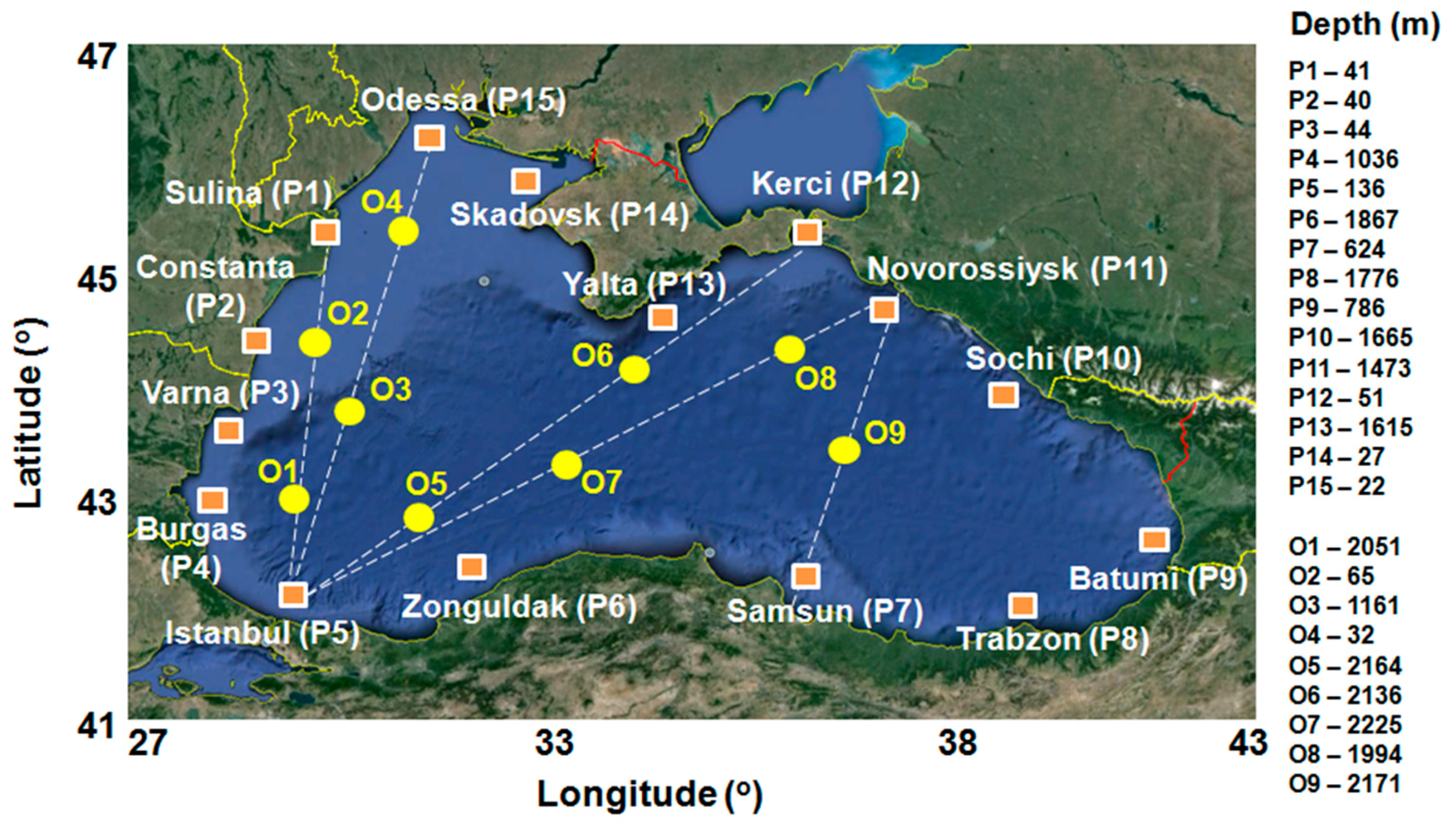
The Black Sea covers an area of 422,000 km2. The maximum distance between its coasts is 1150 km along the west-east direction, as compared to 580 km stretching from north to south. The average water depth is around 1240 m, while a maximum of 2210 m is noticed in the offshore. As regards the bathymetry of the sea, a wide shelf area located in the north-western sector, where the water depth is around 50 m, can be noticed. The remaining area (60%) is associated with an abyssal plain, where depths below 2000 m are encountered. Although this is an inland sea, it is connected to the Marmara and Azov seas, through the Bosporus and Kerch straits. These represent important links for the maritime activities [27].
The geographical position and the correspondent depth of the points that were selected for the analysis are presented in Figure 1 and Table 1. The nearshore sites (denoted from P1 to P15) are defined in the vicinity of the coastal areas, being located at a distance of about 30 km from the nearest harbor. More precisely, the sites are divided between: Romania (Sulina and Constanta), Bulgaria (Varna and Burgas), Turkey (Istanbul, Zonguldak, Samsun, and Trabzon), Georgia (Batumi), Russia (Sochi, Novorossiysk, Kerci, and Yalta), and Ukraine (Skadovsk and Odessa). The depths of the nearshore sites range between a maximum of 1867 m at Zonguldakis, and a minimum of 22 m at Odessa. The offshore sites (group O1-O9) were considered along the major shipping routes, which connect the coastal cities Sulina, Odessa, Istanbul, Kerci, or Novorossiysk [37]. The smallest water depths are noticed in the vicinity of the reference points O2 and O4, when compared to the other offshore sites where the water depth exceeds 2000 m.
2.2. Dataset
In this work, four wind and wave datasets covering a time period from 1987 to 2009 will be analyzed. As regards the wind conditions, the first dataset is related with the reanalysis wind fields that were provided by NCEP-CFSR (U.S. National Centers for Environmental Prediction—Climate Forecast System Reanalysis), which will be further denoted as NCEP. This is based on a coupled forecast system model, which combines a spectral atmospheric model and the MOM (Modular Ocean Model) from GFDL (U.S. Geophysical Fluid Dynamics Laboratory), version 4p0d [38,39]. Various satellite measurements were considered for the assimilation system in order to improve the data [40].
Another dataset of wind fields are obtained from EURO-CORDEX [41,42], the European branch of CORDEX (Coordinated Regional Downscaling Experiment) project. These are the hindcast (evaluation) wind fields that are simulated by a RCM (Regional Climate Model), namely RCA4 (Rossby Centre regional climate model, [43]) from SMHI (Swedish Meteorological and Hydrologic Institute), forced with initial and lateral boundary conditions that are provided by ECMWF ERA-Interim. The data simulated with RCA4 have a fine resolution of 0.11 degrees and they will be further denoted as EUR11 [44]. All of the wind fields are provided at 10 m height and U10 denotes the wind speed.
On the other hand, the features of the wave climate in the Black Sea are assessed while using information from two datasets that is based on simulation results from SWAN model driven with the above-mentioned wind fields. In both SWAN simulations the same bathymetry (provided by General Bathymetric Chart of the Oceans) and model settings were used. The computational domain was chosen to coincide with the bathymetric grid and it has 176 points in the x-direction and 76 points in the y-direction equally spaced in both directions. The lower left corner (27.5° E/41.0° N) represents the origin of the system that covers 14° in longitude and 6° in latitude. In the spectral space, 36 directions (providing a 10° resolution) and 30 frequencies (ranging between 0.05 and 1.0 Hz) are considered. All of the simulations were performed in the non-stationary mode with a time step of 10 min. Some additional information that is related to the physical processes activated in the SWAN simulations are provided [28]. More details regarding the parameters and the characteristics of the databases considered in this work are presented in Table 2, where the subscripts of SWANNCEP and SWANEUR11 indicate the wind fields that are used to force the wave model.
3. Results
3.1. Analysis of the Wind Conditions
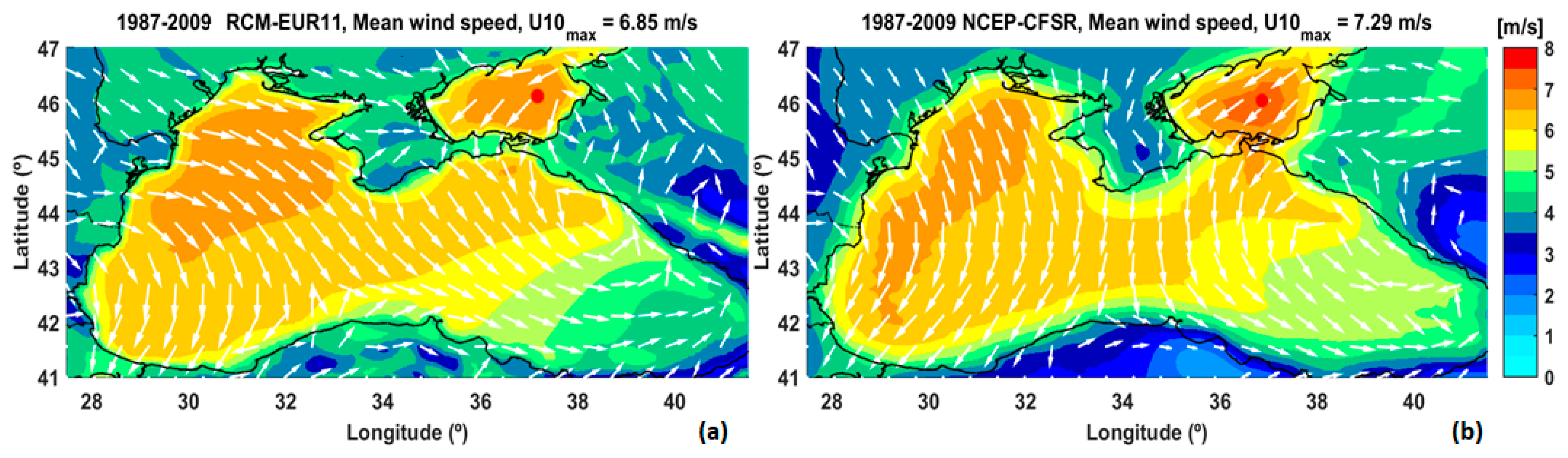
For the wind climate analysis, the average values of the wind speed (U10) and of the wind direction have been computed while considering the total data for the 23-year period (1987–2009). In Figure 2, the spatial distributions are presented, where the wind direction is indicated by white arrows that are scaled with the U10 background field. The position in the field of the maximum U10 mean value is indicated by a red circle, while the borders between the surrounding countries are represented by black lines. The coastal line of the Black Sea basin is also marked with black color. For both the wind fields considered, the maximum values are located over the Azov Sea, with the highest value in the case of NCEP (7.29 m/s). In general, the patterns of the spatial distributions are similar, with higher values of the U10 mean in the western part of the basin and in the Azov Sea. In the southern part of the basin (near to Turkish coast) the NCEP U10 means have lower values than those computed from EUR11. Some differences of the mean wind direction are observed over the entire basin.
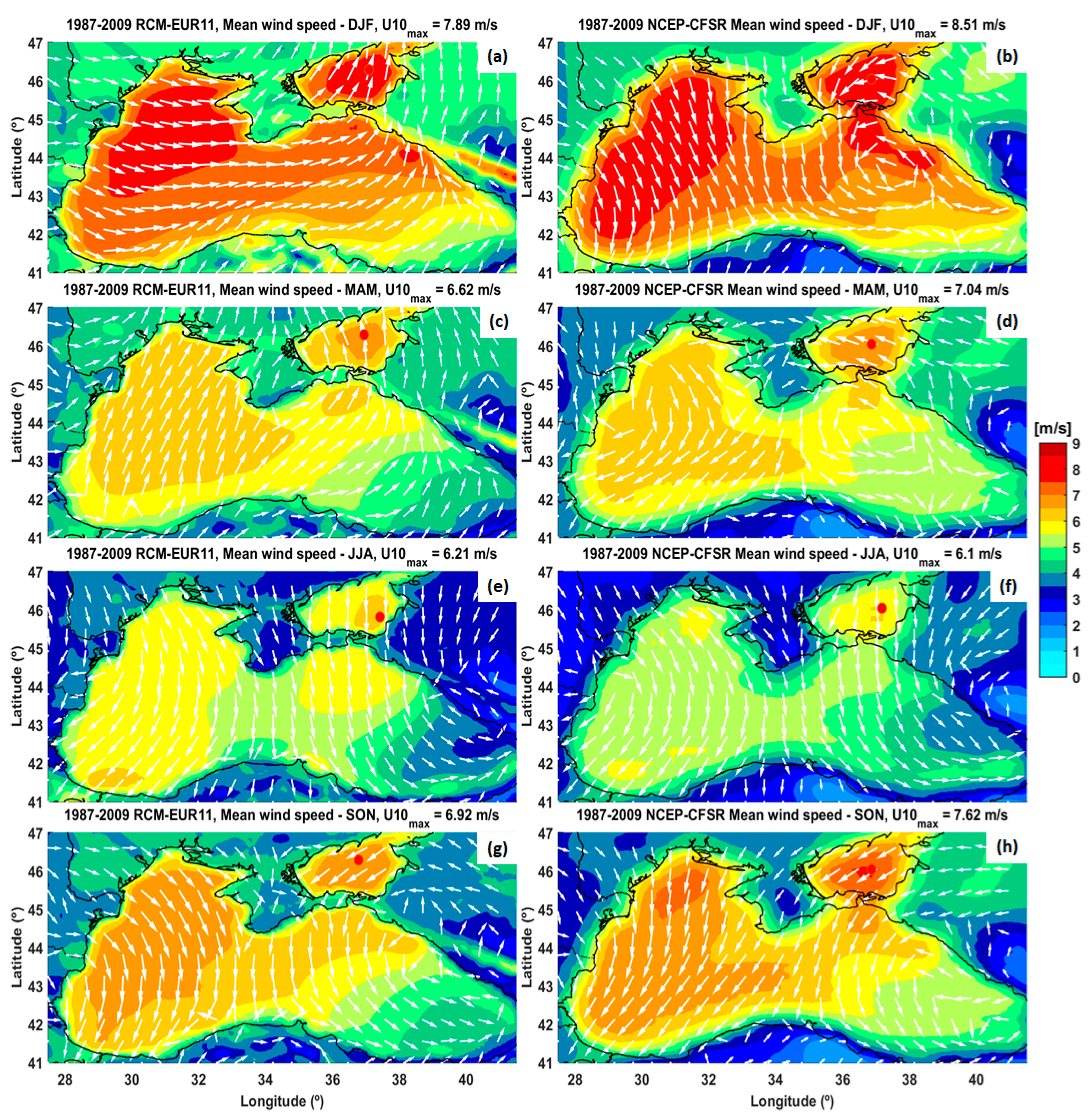
The wind speeds over the Black Sea basin present a seasonal variability that can be easily observed from the seasonal spatial distributions illustrated in Figure 3. The seasonal average values of U10 were computed by extracting from the total the information data following the seasonal partition: winter—DJF (December-January-February), spring—MAM (March-April-May), summer—JJA (June-July-August), and autumn—SON (September-October-November). At this point, it has to be highlighted that the speed of seasonally averaged wind is not the same as the seasonal average of wind speed.
As it can be observed from the spatial distributions presented in Figure 3, the maximum values of the mean U10, for both wind data and all seasons, are always located over the Azov Sea. The highest maximum values are encountered for NCEP wind speeds (higher with about 0.5 m/s than EUR11), except in summer time. For both data sources and in all seasons, higher U10 means are encountered over the Azov Sea and in the western side of the basin. In these areas, the wind directions also have a well-defined pattern, except in the spring time for NCEP winds. In the southern part of the basin, the NCEP U10 means maintain for all seasons the same pattern, as in the case of the total data, namely lower values than those that are computed from EUR11. Significant differences in terms of mean wind directions are encountered in DJF and MAM between NCEP and EUR11. In a small area from the north-eastern part of the basin, which is located near to the Kerch Strait, U10 means present also high values in all seasons.
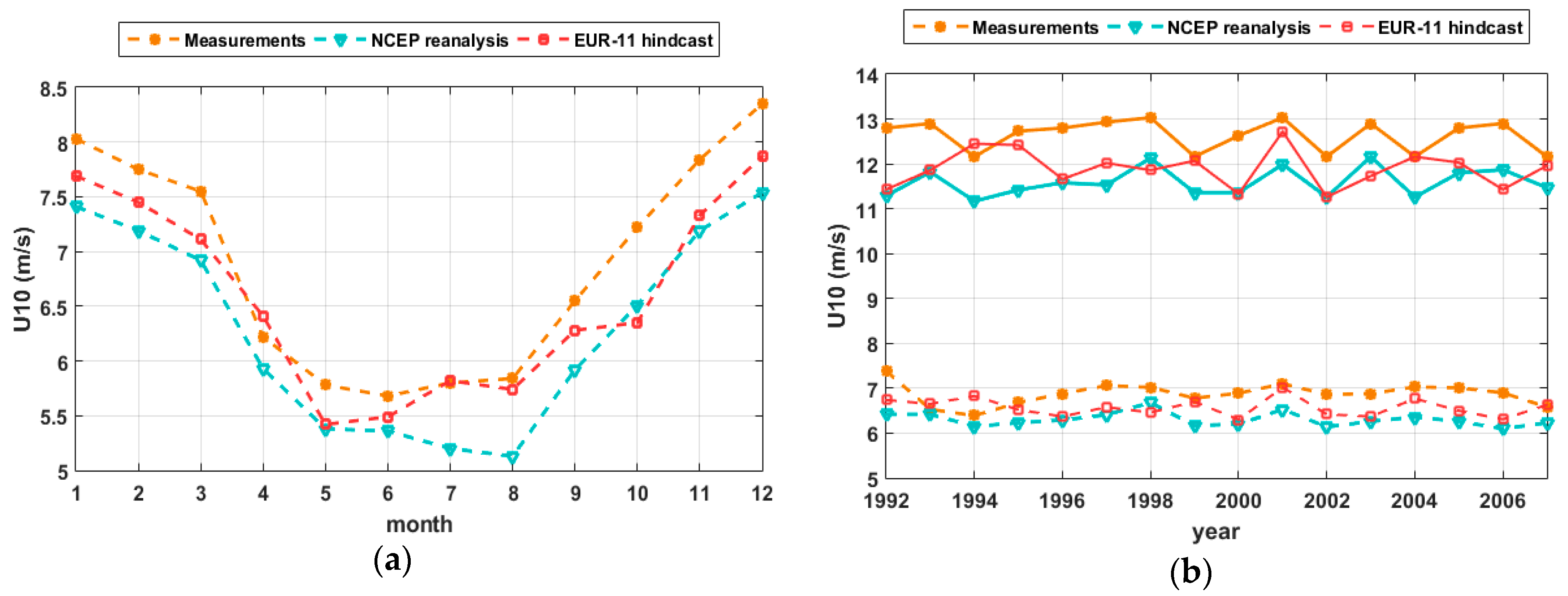
In order to ascertain the capability of the wind fields to represent the wind climate in a certain location, a comparison with the wind climate determined from measurements was also made. Since the EUR11 wind fields were provided by a RCM model, only statistical comparisons between simulated parameters and the present climate can be performed [45]. These typically include measures that summarize features of the climatological mean state and others that summarize temporal variability [46]. The wind speeds recorded for a 16-year period (1992–2007) at the Gloria Platform (44.52° N/29.57° E) located 30 km offshore from the Romanian shore are considered [30]. Comparisons between U10 measured and simulated at the location of the Gloria platform are presented in Figure 4.
Generally, at the location of Gloria platform, the measurements are slightly higher than the simulations; with the EUR11 mean values being in the middle. The monthly means of U10 presented in Figure 4a clearly show the seasonal variation of the wind speed magnitude. In the summer months, the U10 means computed from EUR11 are very close to the measurements, and higher with about 1 m/s than NCEP. As shown in the graphs that are represented by dashed lines in Figure 4b, the annual U10 means are ranging from 6 m/s to 7 m/s for all data sources. In the same figure, the 95th percentiles of U10 are represented by solid lines and they reach values from 11 m/s to 13 m/s. From Figure 4b it can also be observed that no significant trends seem to be present in the annual means and 95th percentile of the measured and simulated wind speed.
The analysis of the U10 features in terms of mean values, 75th percentile and 95th percentile along the ship routes represents the next step. Thus, Figure 5 illustrates the values of the foregoing terms computed for the EUR11 and NCEP datasets in each site mentioned in Table 1 and represented in Figure 1. The two data sets seem to be in good agreement, with very close values for average values and 75th percentile, while for 95th percentile higher values are computed in the case of the NCEP wind speeds.
From Figure 5, it is also observed that the previous remarks are not valid for some sites that are located in the nearshore of the southern Black Sea coast, especially the sites P5, P6, P7, and P8. In these locations the means, the 75th percentile and 95th percentile values are always lower for the NCEP winds. This feature regarding lower values of the NCEP wind speeds in the south was also mentioned in the analysis of the spatial distributions.
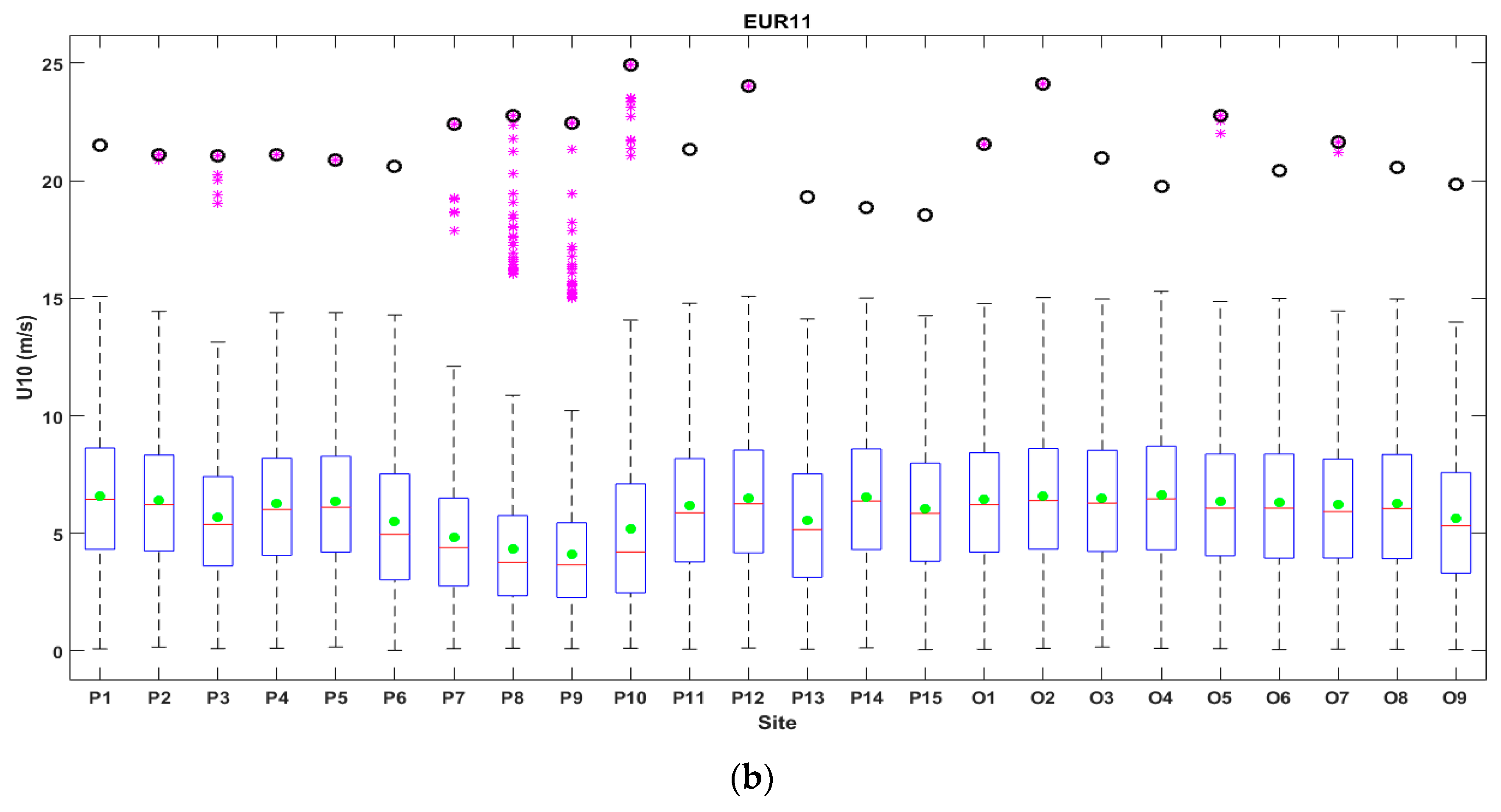
In order to have more information about the statistical characteristics of U10 in each site, the box-and-whisker plots were designed for both for the EUR11 and NCEP datasets and these are presented in Figure 6. Each box encloses the interquartile range, from the first quartile (or 25th percentile) to third quartile (or 75th percentile) of data [47,48]. The red line drawn in the box represents the median value (or 50th percentile), while the green circle is the mean value. The whiskers spanning from a minimum value, which is the smallest data point within 1.5 interquartile ranges from the first quartile, to a maximum value that is the largest data point within 1.5 interquartile ranges from the third quartile. In order to have some information about the extreme values encountered in each data set, the values beyond the upper outer fence were represented with magenta stars, while with black circle the maximum value is marked.
Always the mean values are slightly higher than the median, which means a positive skewness, also indicating that the influence of the outliers on the mean values is reduced. It can be observed that the extreme outliers (represented with magenta stars) are more present in the NCEP wind (except P12 and O4) than in the EUR11 wind, where they are encountered only in half of the sites. In both data sets, the most affected sites by the extreme outliers are P3 in the west of the sea basin, while in the east P7, P8, P9, and P10. This probably is influenced by the complicated orography that characterizes the eastern coast of the Black Sea [30]. In the case of the EUR11 wind, the extreme outliers are not present in the data sets from the offshore locations and also in the northern half of the basin. As regards the maximum values, for the NCEP winds they reach 25 m/s at various sites, while for the EUR11 wind, they are around 20 m/s at the most of the sites.
As mentioned, significantly lower values of average U10 are encountered in the south, more precisely the smallest wind speeds (around 3.7 m/s) being encountered in the vicinity of the sites P7 and P8 for the NCEP wind. From the nearshore sites it results that P1, P2, P4, and P12 are defined by more important values, which may reach a maximum of 6.6 m/s, value that is comparable to those that are encountered in the offshore sites. From the Figure 2 and Figure 3, it can be easily observed that in the south-western part of the Black Sea basin the average values of the NCEP wind are slowly lower than those of EUR11. Not the same thing can be said in the case of the offshore areas. This is also confirmed by the comparison presented in Figure 5, where it can be observed the difference existent between the nearshore and offshore points. In the offshore points, the U10 NCEP average values are higher than those from EUR11.
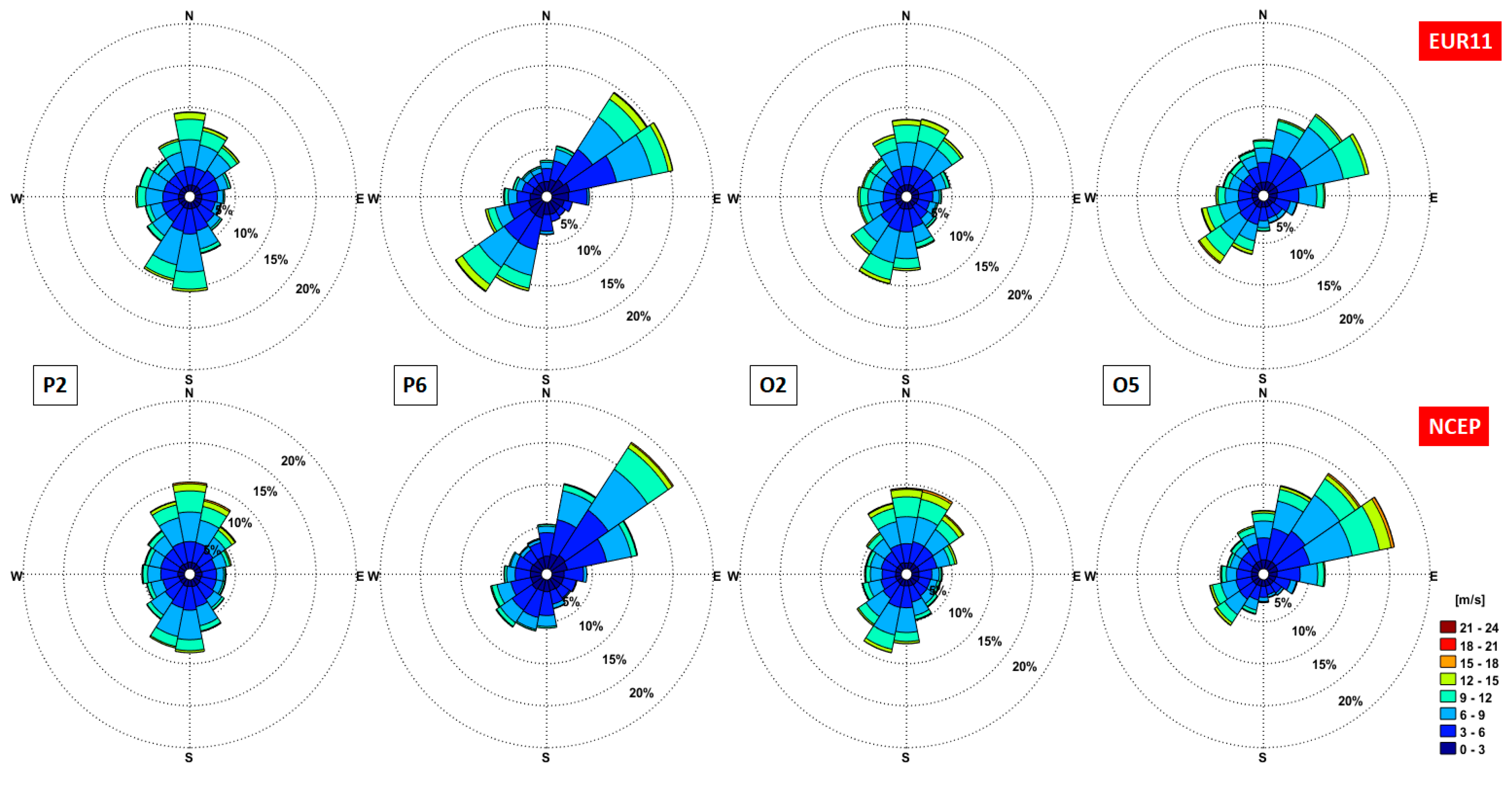
In all of the sites located along the shipping routes, the directional distributions of the wind speeds were also computed based on the data provided by both datasets. The analysis of all distributions indicated that only in the sites from southern part of the basin (generally below the latitude 43° N) some differences regarding the dominant wind directions are encountered. In Figure 7, some directional distributions of U10 are illustrated for sites that are located in nearshore and offshore. Thus, it can be observed that in P2 and O2, which are located on the western side of the Black Sea basin, the directional distributions of the U10 classes are almost identical for the EUR11 and NCEP datasets. Not the same feature can be noticed for the directional distributions computed in the sites P6 and O5. These are also located in the western side of the basin, but in the southern part. An increase in the percentage (about 5%) of the wind blowing from the south-west, together with a decrease of winds blowing from the north-east, is observed in the site P6 for the EUR11 wind speeds as compared with the NCEP data. Likewise, the directional distributions are changed in the reference point O5, following the same features as in the point P6.
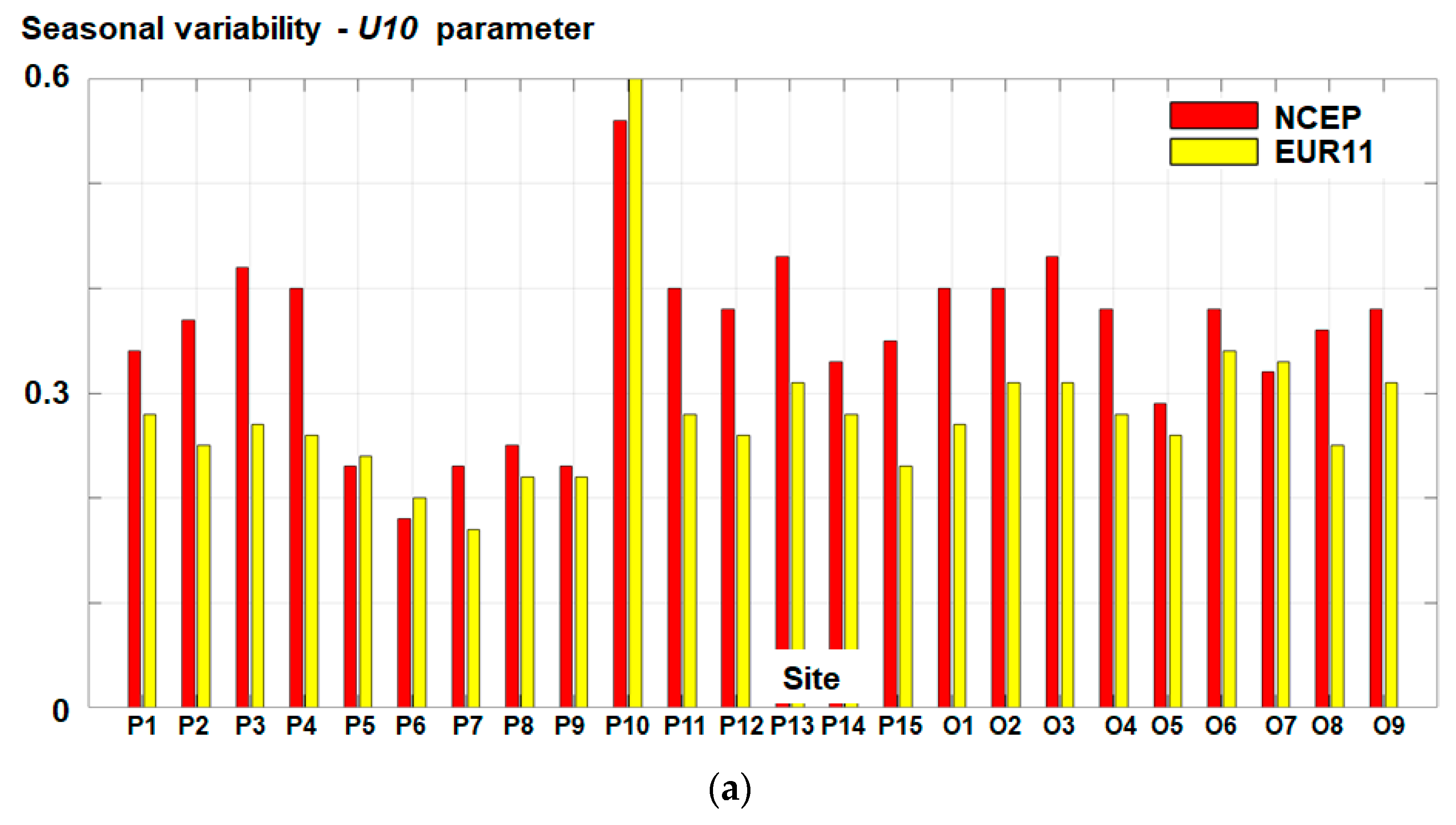
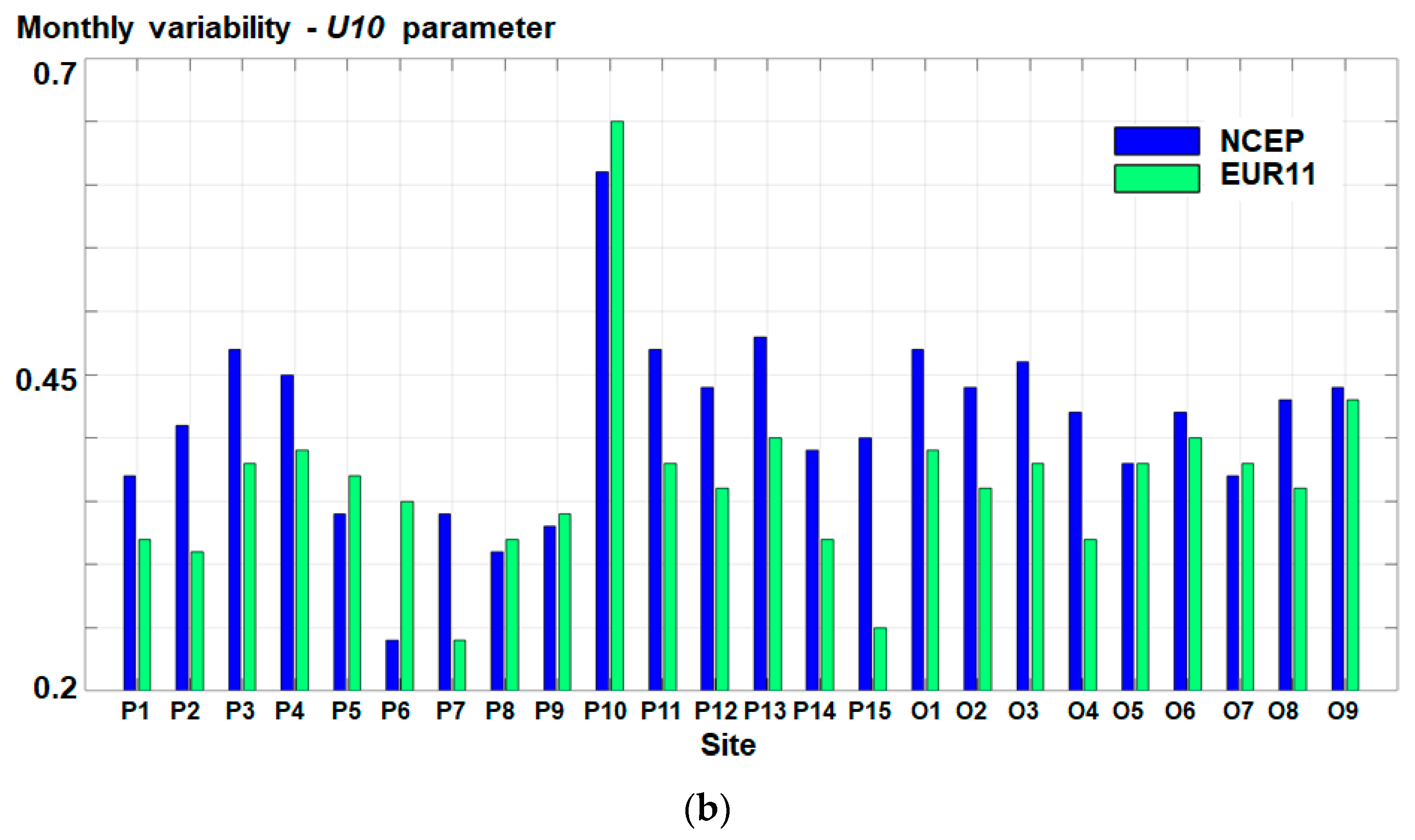
As a next step, the seasonal (SV) and monthly (MV) variability of the wind speeds along the ship routes will be also assessed. The information provided by the seasonal and monthly variability indexes can help for a better description of the variation in time of the wind speeds. The seasonal partition is the same as in the spatial distributions. The SV and MV indexes are defined as the differences between the most energetic season/month and the least energetic season/month divided by the yearly average value evaluated over the whole dataset. Usually, in the northern hemisphere, winter (DJF) is the most energetic season, while summer (JJA) is least energetic [49]. The following equations were used to assess the SV and MV index [50]:
where: PSmax—the most energetic season; PSmin—the least energetic season; Paverage—the yearly average value computed for the entire dataset; PMmax—the most energetic month; PMmin—the least energetic month.
Figure 8 shows the SV and MV indexes computed in each site while considering EUR11 and NCEP wind speeds, respectively. The NCEP data present, in general, a higher variability, both seasonal and monthly. Only some points from the south-eastern part of the basin do not have the above-mentioned features. Thus, the EUR11 wind speeds present a higher variability than those from NCEP in the nearshore sites P5, P6, and P10 and in the offshore site O7, for both indexes. As regards the monthly variability, also in P8 and P9 it can be found the same feature, as previously mentioned.
3.2. Analysis of the Wave Conditions
For the wave conditions, only the significant wave height (Hs) parameter is evaluated, by considering the simulation results from SWANNCEP and SWANEUR11. The SWAN model simulations also provide information about the Hs spatial distribution corresponding to the same time interval, as in the case of the wind speeds (1987–2009).
The SWAN model calibration and validation in the Black Sea was made in some previous studies against both in-situ and altimeter measurements [28,31,51], and the statistical results show a good agreement between the simulated and the measured values, indicating the fact that reliable wave predictions are provided by the modeling system. In all of the above-mentioned studies, the NCEP wind fields were considered to drive the wave model. Moreover, the settings used for SWAN model simulations and also the bathymetry are the same as in the previous studies. The fact that NCEP wind fields are appropriate to force the SWAN model is also confirmed by the results that were obtained in other studies [18,24,52,53].
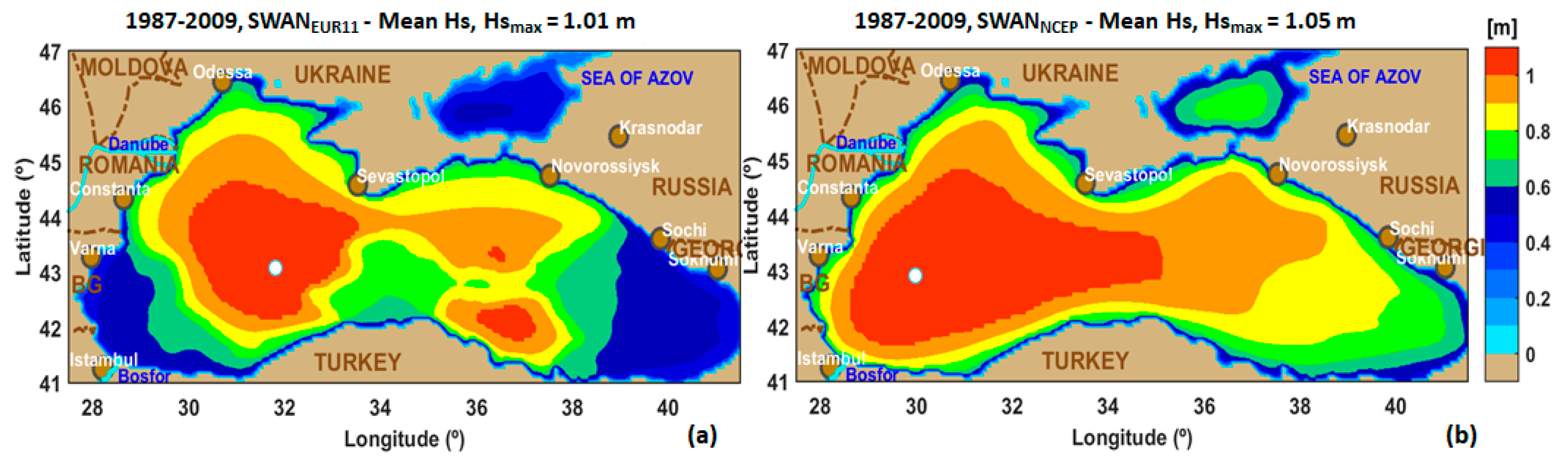
Figure 9 presents the spatial distribution of the average Hs values resulted from the SWAN simulations, while the Hs fields corresponding to the seasons have been represented in Figure 10. When comparing the maps presented in Figure 8, it can be observed that the maximum values are almost the same (about 1 m), while the positions of these maxims are also located in the western side of the basin.
Some differences can be noticed in the spatial distribution of the significant wave height fields that are presented in Figure 9. Thus, the areas from the south-west and south-east of the Black Sea basin (in front of the Bulgarian, Turkish, and Georgian coastlines) show lower Hs values for the SWANEUR11 results. The same decrease of the Hs values is also observed in the Azov Sea. A better agreement between both fields exists in the central part of the Black Sea basin.
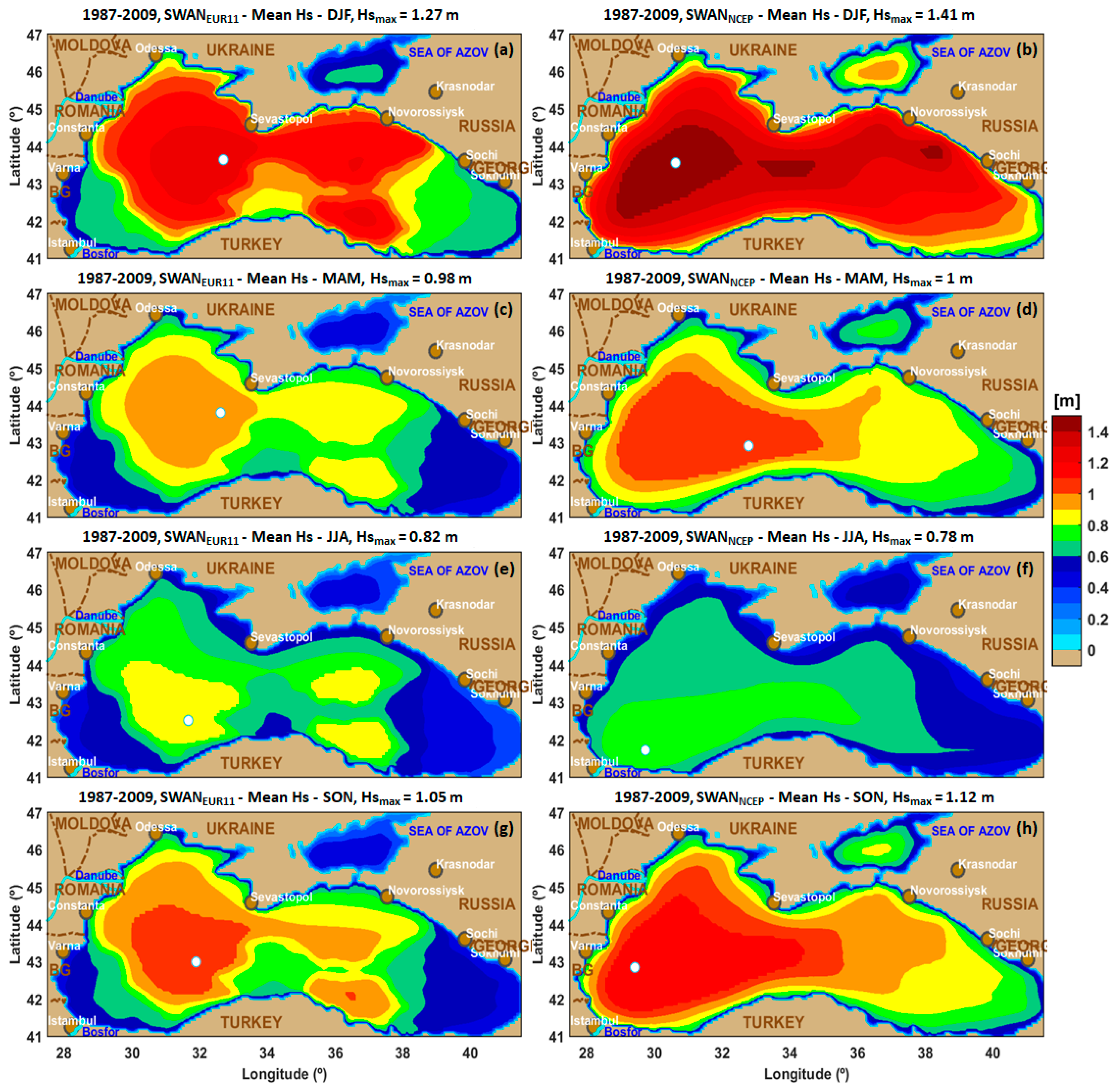
These differences observed in the Hs spatial distributions are a consequence of the changes in the wind directions. The changes in the wind direction between the NCEP and EUR11 data sets can be observed better in the maps that are presented in Figure 3, where the wind vectors indicate the seasonal average wind direction. Looking especially to the winter maps (Figure 3a,b, when the highest wind speeds are encountered, the average wind directions are different (this difference being about 90°). Thus, in the western side of the basin, the main direction from which the NCEP winds blow is north-northwest. In these conditions, the development of the waves along the fetch is from north to south and in the SWANNCEP results we can notice the highest Hs values occurring near to the Turkish coast (see Figure 10b). The main direction of the EUR11 winds is from west-southwest, and these wind conditions favor the development of the waves from west to east. Through this wave development, the highest Hs values that are simulated by SWANEUR11 are found in central and north-eastern part of the Black Sea basin (see Figure 10a).
As regards the eastern side, also some differences in terms of the wind direction are encountered and these influenced the fetch length for the wave development. Moreover, in this area, the NCEP wind speeds are higher than those from EUR11, and higher local waves were generated. The waves in the Azov Sea are mainly influenced by the local winds, and the differences between the wind speeds are directly reflected in differences regarding the sea states conditions. The seasonal variations in the spatial distributions of the Hs fields maintain the same patterns, as in the case of total data. In wintertime (DJF) the differences between the spatial distributions computed using different databases are more accentuated. The maximum value is 1.27 m for SWANEUR11, while for SWANNCEP this reaches 1.41 m.
Because the SWAN model has already been calibrated and validated, the validation of the wave model was not an objective of this work. However, a comparison between the wave climate based on measurements at the Gloria Platform and those resulted from the SWAN simulations using both wind fields was performed over the period 1999–2007, when measurements are available. The corresponding results are presented in Figure 11.
As in the case of the wind speeds, the seasonality existent also in the Hs features can be observed in Figure 11a. Thus, it can be noticed that in the spring months there is a very good correlation between all of the monthly means (measurements and simulated values), while in autumn and wintertime the measurement means present higher values, followed by the results that are provided by SWANNCEP. In the summer, the monthly means computed for Hs simulated by SWANEUR11 fit very well the measurement means, while SWANNCEP provides lower values. As regards the annual means, they are around 1 m and show a very good correlation between the simulated results, these being slightly lower than the measured means (about 0.05 m). The 95th percentiles of Hs present higher values for the measurements (around 2.5 m). In the case of the simulations, this ranges from 1.98 m to 2.36 m for SWANEUR11, while those that were computed for SWANNCEP are around 2 m (±0.15 m).
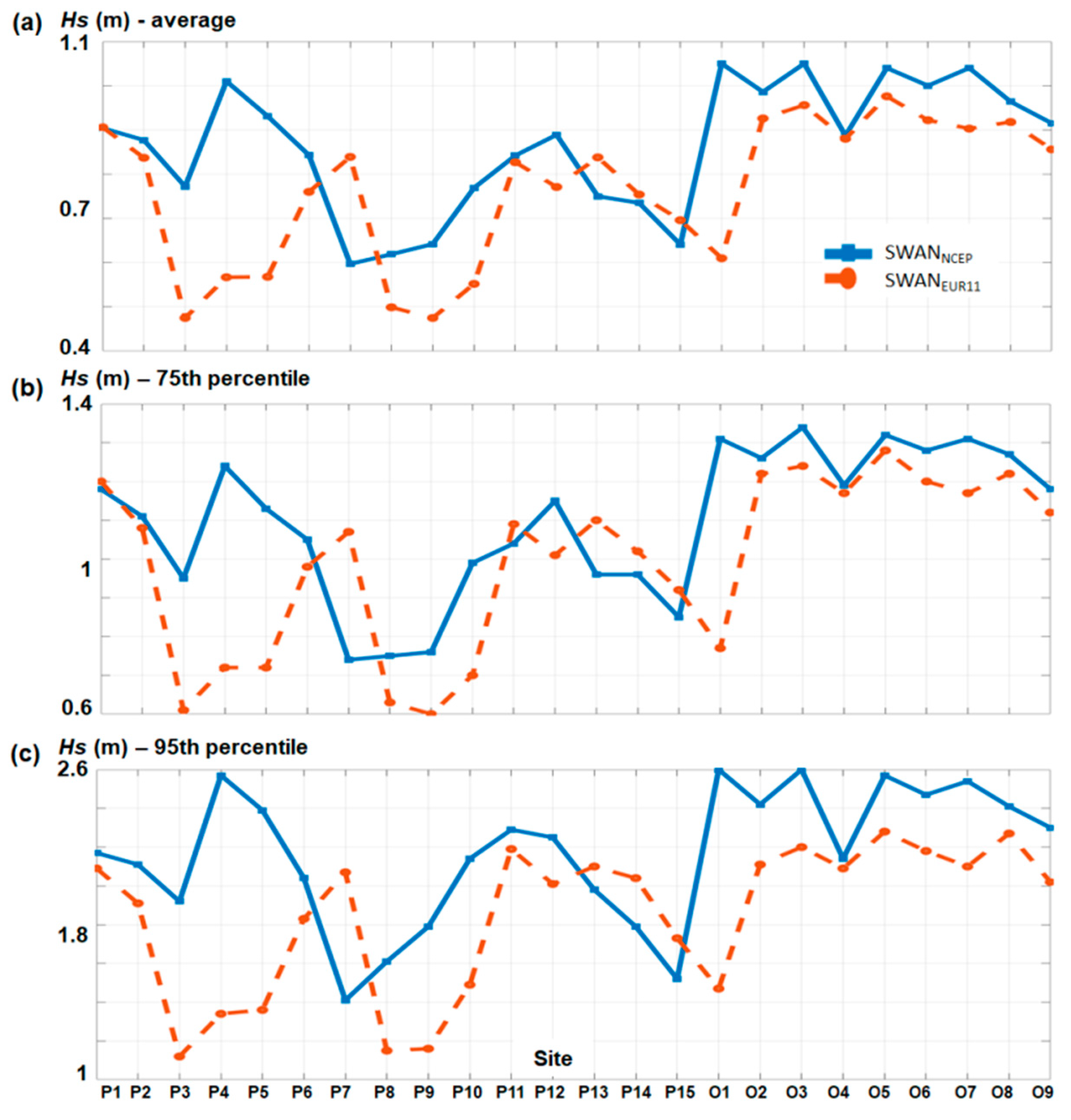
As in the case of the wind speeds, the Hs features were analyzed based on the same terms (mean values, 75th percentile, and 95th percentile), their values being presented in Figure 12. Thus, it can be observed that the graphs have the same behavior for all terms. The SWANEUR11 values are, in general, significantly smaller than the SWANNCEP values, and as expected, the higher differences between two data are encountered in the sites that are located in the south-west and south-east areas of the Black Sea basin (P3, P4, P5, P8, P9, P10, and O1). Some severe variations are observed in the case of the site P4 or O1, respectively. For the SWANEUR11 data, a minimum average value of 0.47 m was computed for the sites P3 and P9, while a maximum of 0.98 m is accounted for the site O3.
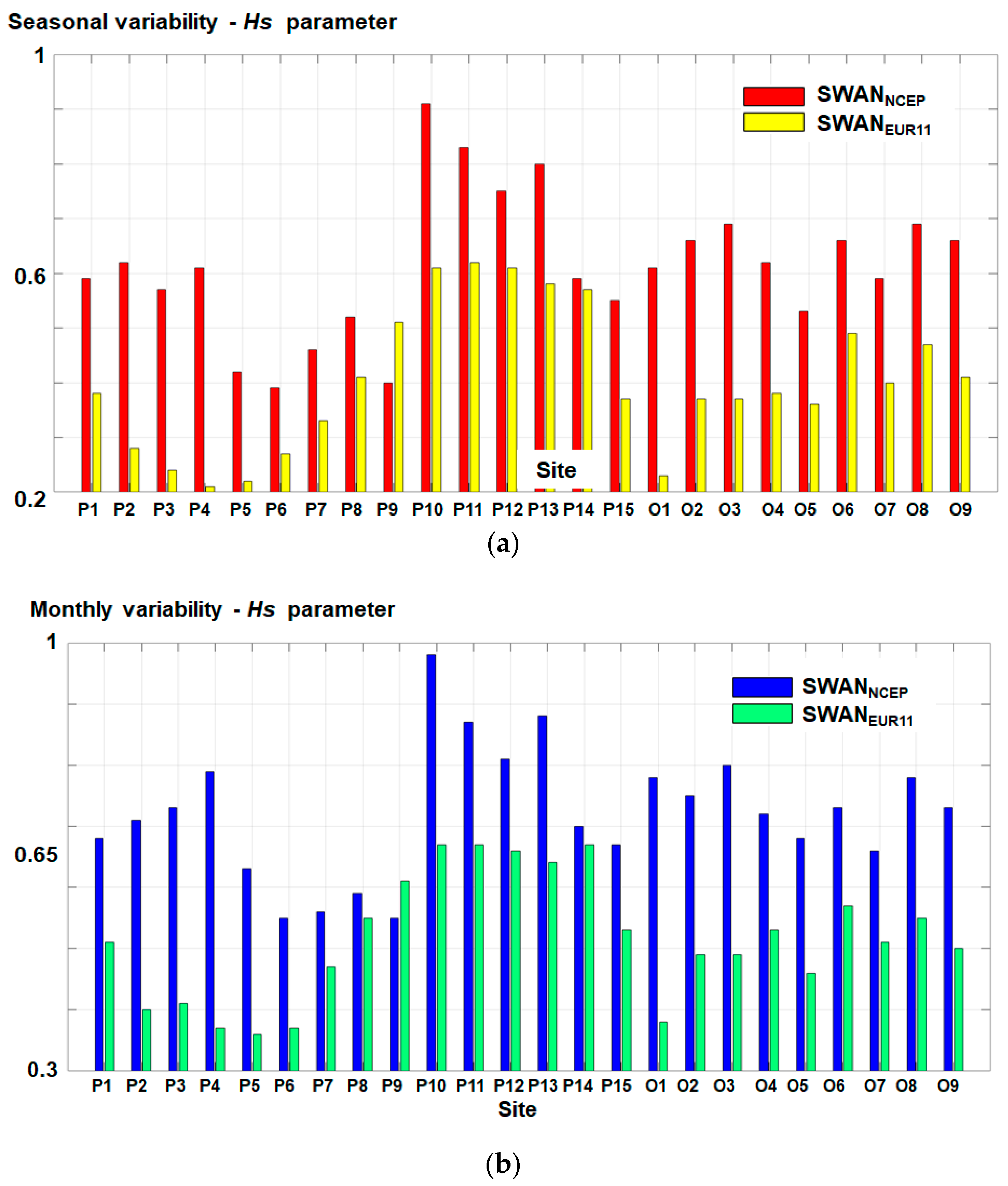
The SV and MV indexes were also computed for Hs in each site, while considering the results from SWANEUR11 and SWANNCEP (see Figure 13). The higher variability of the NCEP wind fields also induced a higher variability of the SWANNCEP wave fields, even more accentuated than for the wind. Thus, in more than 50% of the sites SV index is higher than 0.6. In the north-eastern part of the basin the highest values of SV are noticed (around 0.8). In these sites, the highest SV indexes for SWANEUR11 can also be found, they values reach 0.6. In all of the other points, the SV indexes for SWANEUR11 are lower than 0.5, in some points (P4, P5, and O1) presenting even lower values (around 0.2). As regards the MV index, the same pattern observed for the SV index is maintained, but with higher values result for MV. In P10, the MV index is near 1 for SWANNCEP, while for SWANEUR11 is 0.65.
4. Conclusions
In the present study, the wind and wave climate in the Black Sea area was assessed. This is based on data provided over a 23-year period (1987–2009) by two different sources. Comparisons between both datasets have been also carried out. A particular attention was given in the present work to the sites that are located along the major maritime routes and harbors.
The analysis of the spatial distributions of the wind speed and of the significant wave height computed as means of the total and seasonal data show a good correlation between the two datasets, especially in the western and central sides of the basin. The offshore sites seem to show a better correlation between the two datasets for both wind and waves.
Furthermore, comparisons of the annual and monthly means computed for the simulated U10 and Hs were made against the measured means of the same parameters. Generally, a good agreement was observed, the measurement means being slightly higher than the simulated means, especially in the wintertime. In the summer time, the NCEP wind speeds and the SWANNCEP significant wave heights present lower values than the measurements, while the EUR11 wind speeds and the SWANEUR11 significant wave heights show a very good agreement with the measurements.
A good agreement between the average values of the wind data provided by the different datasets can be found in the nearshore sites, except for the points that are located in the southern part of the Black Sea. The extreme values show the same trends as those encountered for the average values.
The results that were obtained in this study are useful for the evaluation of the wind and wave climate in the Black Sea based on various datasets, but it has to be highlighted that also represents a first step in the utilization of the RCM wind fields to simulate the sea state conditions in the Black Sea. The work is still ongoing and future studies related to the wind variability will be performed considering various approaches, as for example, that given in [54]. In our opinion, the results are encouraging for further simulations regarding the future climate projections of the wave conditions in the Black Sea.
Author Contributions
L.R. has guided this research, processed the spatial data and writes the manuscript. A.B.R. collected and processed the wind and wave data, caring also the literature review. F.O. performed the statistical analysis and interpreted the results. The final manuscript has been approved by all authors.
Funding
This work was supported by a grant of Ministry of Research and Innovation, CNCS—UEFISCDI, project number PN-III-P4-ID-PCE-2016-0028, within PNCDI III.
Acknowledgments
The authors would like also to express their gratitude to the reviewers for their constructive suggestions and observations that helped in improving the present work.
Conflicts of Interest
The authors declare no conflict of interest.
References
- Lyratzopouoou, D.; Zarotiadis, G. Black Sea: Old Trade Routes and Current Perspectives of Socioeconomic Co-operation. Procedia Econ. Financ. 2014, 9, 74–82. [Google Scholar] [CrossRef]
- Onea, F.; Rusu, L. A Long-Term Assessment of the Black Sea Wave Climate. Sustainability 2017, 9, 1875. [Google Scholar] [CrossRef]
- Onea, F.; Raileanu, A.; Rusu, E. Evaluation of the Wind Energy Potential in the Coastal Environment of Two Enclosed Seas. Adv. Meteorol. 2015, 808617. [Google Scholar] [CrossRef]
- Davy, R.; Gnatiuk, N.; Pettersson, L.; Bobylev, L. Climate change impacts on wind energy potential in the European domain with a focus on the Black Sea. Renew. Sustain. Energy Rev. 2018, 81, 1652–1659. [Google Scholar] [CrossRef] [Green Version]
- Allenbach, K.; Garonna, I.; Herold, C.; Monioudi, I.; Giuliani, G.; Lehmann, A.; Velegrakis, A.F. Black Sea beaches vulnerability to sea level rise. Environ. Sci. Policy 2015, 46, 95–109. [Google Scholar] [CrossRef]
- Limber, P.W.; Barnard, P.L. Coastal knickpoints and the competition between fluvial and wave-driven erosion on rocky coastlines. Geomorphology 2017. [Google Scholar] [CrossRef]
- Nastase, G.; Serban, A.; Nastase, A.F.; Dragomir, G.; Brezeanu, A.I.; Iordan, N.F. Hydropower development in Romania. A review from its beginnings to the present. Renew. Sustain. Energy Rev. 2017, 80, 297–312. [Google Scholar] [CrossRef]
- Kosyan, R.D.; Velikova, V.N. Coastal zone—Terra (and aqua) incognita—Integrated Coastal Zone Management in the Black Sea. Estuar. Coast. Shelf Sci. 2016, 169, A1–A16. [Google Scholar] [CrossRef]
- Tong, S.; Mather, P.; Fitzgerald, G.; McRae, D.; Verrall, K.; Walker, D. Assessing the Vulnerability of Eco-Environmental Health to Climate Change. Int. J. Environ. Res. Public Health 2010, 7, 546–564. [Google Scholar] [CrossRef] [PubMed] [Green Version]
- Bhore, S.J. Paris Agreement on Climate Change: A Booster to Enable Sustainable Global Development and Beyond. Int. J. Environ. Res. Public Health 2016, 13, 1134. [Google Scholar] [CrossRef] [PubMed]
- Dodla, V.B.; Desamsetti, S.; Yerramilli, A. A Comparison of HWRF, ARW and NMM Models in Hurricane Katrina (2005) Simulation. Int. J. Environ. Res. Public Health 2011, 8, 2447–2469. [Google Scholar] [CrossRef] [PubMed] [Green Version]
- Jacobson, M.Z. Fundamentals of Atmospheric Modeling, 2nd ed.; Cambridge University Press: Cambridge, UK, 2005; ISBN 978-0-521-54865-6. [Google Scholar]
- Rogers, W.E.; Dykes, J.D.; Wittmann, P.A. US Navy global and regional wave modeling. Oceanography 2014, 27, 56–67. [Google Scholar] [CrossRef]
- Holthuijsen, L.H. Waves in Oceanic and Coastal Waters; Cambridge University Press: Cambridge, UK, 2010. [Google Scholar]
- Rusu, L.; Soares, C.G. Evaluation of a high-resolution wave forecasting system for the approaches to ports. Ocean Eng. 2013, 58, 224–238. [Google Scholar] [CrossRef]
- Cherneva, Z.; Andreeva, N.; Pilar, P.; Valchev, N.; Petrova, P.; Guedes Soares, C. Validation of the WAMC4 wave model for the Black Sea. Coast. Eng. 2008, 55, 881–893. [Google Scholar] [CrossRef]
- Koletsis, I.; Kotroni, V.; Lagouvardos, K.; Soukissian, T. Assessment of offshore wind speed and power potential over the Mediterranean and the Black Seas under future climate changes. Renew. Sustain. Energy Rev. 2016, 60, 234–245. [Google Scholar] [CrossRef]
- Kislov, A.V.; Surkova, G.V.; Arkhipkin, V.S. Occurence Frequency of Storm Wind Waves in the Baltic, Black, and Caspian Seas under Changing Climate Conditions. Russ. Meteorol. Hydrol. 2016, 41, 121–129. [Google Scholar] [CrossRef]
- Velea, L.; Bojariu, R.; Cica, R. Occurrence of Extreme Winds over the Black Sea during January Under Present and Near Future Climate. Turk. J. Fish. Aquat. Sci. 2014, 14, 973–979. [Google Scholar] [CrossRef]
- Onea, F.; Rusu, E. An Evaluation of the Wind Energy in the North-West of the Black Sea. Int. J. Green Energy 2014, 11, 465–487. [Google Scholar] [CrossRef]
- Argin, M.; Yerci, V. Offshore wind power potential of the Black Sea region in Turkey. Int. J. Green Energy 2017, 14, 811–818. [Google Scholar] [CrossRef]
- Kucukali, S.; Dinckal, C. Wind energy resource assessment of Izmit in the West Black Sea Coastal Region of Turkey. Renew. Sustain. Energy Rev. 2014, 30, 790–795. [Google Scholar] [CrossRef]
- Rusu, L.; Butunoiu, D. Evaluation of the Wind Influence in Modeling the Black Sea Wave Conditions. Environ. Eng. Manag. J. 2014, 13, 305–314. [Google Scholar]
- Van Vledder, G.P.; Akpınar, A. Wave model predictions in the Black Sea: Sensitivity to wind fields. Appl. Ocean Res. 2015, 53, 161–178. [Google Scholar] [CrossRef]
- Lin-Ye, J.; García-León, M.; Gràcia, V.; Ortego, M.I.; Stanica, A.; Sánchez-Arcilla, A. Multivariate hybrid modelling of future wave-storms at the northwestern Black Sea. Water 2018, 10, 221. [Google Scholar] [CrossRef]
- Booij, N.; Ris, R.C.; Holthuijsen, L.H. A third-generation wave model for coastal regions: 1. Model description and validation. J. Geophys. Res. 1999, 104, 7649–7666. [Google Scholar] [CrossRef] [Green Version]
- Divinsky, B.V.; Kosyan, R.D. Spatiotemporal variability of the Black Sea wave climate in the last 37 years. Cont. Shelf Res. 2017, 136, 1–19. [Google Scholar] [CrossRef]
- Rusu, L. Assessment of the Wave Energy in the Black Sea Based on a 15-Year Hindcast with Data Assimilation. Energies 2015, 8, 10370–10388. [Google Scholar] [CrossRef] [Green Version]
- Rusu, E. Wave energy assessments in the Black Sea. J. Mar. Sci. Technol. 2009, 14, 359–372. [Google Scholar] [CrossRef]
- Rusu, L.; Bernardino, M.; Guedes Soares, C. Wind and wave modelling in the Black Sea. J. Oper. Oceanogr. 2014, 7, 5–20. [Google Scholar] [CrossRef] [Green Version]
- Rusu, L.; Butunoiu, D.; Rusu, E. Analysis of the Extreme Storm Events in the Black Sea Considering the Results of a Ten-Year Wave Hindcast. J. Environ. Prot. Ecol. 2014, 15, 445–454. [Google Scholar]
- Erselcan, İ.Ö.; Kükner, A. A numerical analysis of several wave energy converter arrays deployed in the Black Sea. Ocean Eng. 2017, 131, 68–79. [Google Scholar] [CrossRef]
- Akpınar, A.; Kömürcü, M.İ. Wave energy potential along the south-east coasts of the Black Sea. Energy 2012, 42, 289–302. [Google Scholar] [CrossRef]
- Min’kovskaya, R.Y. Contamination of the Black Sea surface water layer with oil hydrocarbons. Russ. Meteorol. Hydrol. 2014, 39, 705–712. [Google Scholar] [CrossRef]
- Lavrova, O.Y.; Mityagina, M.I. Satellite monitoring of oil slicks on the Black Sea surface. Izv. Atmos. Ocean. Phys. 2013, 49, 897–912. [Google Scholar] [CrossRef]
- Gasparotti, C.; Rusu, E. Methods for the risk assessment in maritime transportation in the Black Sea basin. J. Environ. Prot. Ecol. 2012, 13, 1751–1759. [Google Scholar]
- Raţă, V.; Gasparotti, C.; Rusu, L. The importance of the reduction of air pollution in the black sea basin. Mech. Test. Diagn. 2017, 7, 5–15. [Google Scholar]
- Griffies, S.M.; Harrison, M.J.; Pacanowski, R.C.; Rosati, A. A Technical Guide to MOM4; GFDL Ocean Group Technical Report No. 5; NOAA/Geophysical Fluid Dynamics Laboratory: Princeton, NJ, USA, 2004; p. 371. [Google Scholar]
- Hodges, K.I.; Lee, R.W.; Bengtsson, L. A comparison of extratropical cyclones in recent reanalyses ERA-Interim, NASA MERRA, NCEP CFSR, and JRA-25. J. Clim. 2011, 24, 4888–4906. [Google Scholar] [CrossRef]
- Saha, S.; Moorthi, S.; Pan, H.-L.; Wu, X.; Wang, J.; Nadiga, S.; Tripp, P.; Kistler, R.; Woollen, J.; Behringer, D.; et al. The NCEP Climate Forecast System Reanalysis. Bull. Am. Meteorol. Soc. 2010, 91, 1015–1058. [Google Scholar] [CrossRef]
- Gutowski, W.J., Jr.; Giorgi, F.; Timbal, B.; Frigon, A.; Jacob, D.; Kang, H.-S.; Raghavan, K.; Lee, B.; Lennard, C.; Nikulin, G.; et al. WCRP COordinated Regional Downscaling EXperiment (CORDEX): A diagnostic MIP for CMIP6. Geosci. Model Dev. 2016, 9, 4087–4095. [Google Scholar] [CrossRef]
- Giorgi, F.; Gutowski, W.J. Regional Dynamical Downscaling and the CORDEX Initiative. In Annual Review of Environment and Resources; Gadgil, A., Tomich, T.P., Eds.; Annual Reviews: Palo Alto, CA, USA, 2015; Volume 40, pp. 467–490. ISBN 978-0-8243-2340-0. [Google Scholar]
- Wang, S.; Dieterich, C.; Döscher, R.; Höglund, A.; Hordoir, R.; Meier, H.M.; Samuelsson, P.; Schimanke, S. Development and evaluation of a new regional coupled atmosphere–ocean model in the North Sea and Baltic Sea. Tellus A Dyn. Meteorol. Oceanogr. 2015, 67, 24284. [Google Scholar] [CrossRef]
- Jacob, D.; Petersen, J.; Eggert, B.; Alias, A.; Christensen, O.B.; Bouwer, L.M.; Braun, A.; Colette, A.; Déqué, M.; Georgievski, G.; et al. EURO-CORDEX: New high-resolution climate change projections for European impact research. Reg. Environ. Chang. 2014, 14, 563–578. [Google Scholar] [CrossRef]
- Soares, P.M.; Lima, D.C.; Cardoso, R.M.; Nascimento, M.L.; Semedo, A. Western Iberian offshore wind resources: More or less in a global warming climate? Appl. Energy 2017, 203, 72–90. [Google Scholar] [CrossRef]
- Hemer, M.A.; Trenham, C.E. Evaluation of a CMIP5 derived dynamical global wind wave climate model ensemble. Ocean Model. 2016, 103, 190–203. [Google Scholar] [CrossRef] [Green Version]
- Wilks, D.S. Statistical Methods in the Atmospheric Sciences, 3rd ed.; International Geophysics Series; Academic Press: Dordrecht, The Netherlands, 2011; 704p, ISBN 978-0-12-385022-5. [Google Scholar]
- Tukey, J.W. Exploratory Data Analysis; Addison-Wesley Publishing Company: Reading, MA, USA, 1977; 688p, ISBN 978-0-20-107616-5. [Google Scholar]
- Cornett, A.M. A Global Wave Energy Resource Assessment. In Proceedings of the Eighteenth International Offshore and Polar Engineering Conference, Vancouver, BC, Canada, 6–11 July 2008. [Google Scholar]
- Rusu, L.; Ganea, D.; Mereuta, E. A joint evaluation of wave and wind energy resources in the Black Sea based on 20-year hindcast information. Energy Explor. Exploit. 2018, 36, 335–351. [Google Scholar] [CrossRef]
- Butunoiu, D.; Rusu, E. A data assimilation scheme to improve the Wave Predictions in the Black Sea. In Proceedings of the IEEE OCEANS 2015-Genova, Genova, Italy, 18–21 May 2015; pp. 1–6. [Google Scholar]
- Akpıar, A.; Bingölbali, B.; Van Vledder, G.P. Wind and wave characteristics in the Black Sea based on the SWAN wave model forced with the CFSR winds. Ocean Eng. 2016, 126, 276–298. [Google Scholar] [CrossRef]
- Akpinar, A.; de León, S.P. An assessment of the wind re-analyses in the modelling of an extreme sea state in the Black Sea. Dyn. Atmos. Oceans 2016, 73, 61–75. [Google Scholar] [CrossRef]
- Hamlington, P.E.; Collins, S.G.; Alexander, S.R.; Kim, K.Y. Effects of climate oscillations on wind resource variability in the United States. Geophys. Res. Lett. 2015, 42, 145–152. [Google Scholar] [CrossRef] [Green Version]
Figure 1.
Map of the Black Sea and the reference sites; the points marked with squares (from P1 to P15) are located near the main harbors, while the points marked with circles (from O1 to O9) are located along the shipping routes.
Figure 1.
Map of the Black Sea and the reference sites; the points marked with squares (from P1 to P15) are located near the main harbors, while the points marked with circles (from O1 to O9) are located along the shipping routes.

Figure 2.
The averaged wind speed is represented in the background, while the wind vectors indicate the average wind direction over the Black Sea: (a) EUR11, (b) NCEP.
Figure 2.
The averaged wind speed is represented in the background, while the wind vectors indicate the average wind direction over the Black Sea: (a) EUR11, (b) NCEP.

Figure 3.
The seasonal averaged wind speed is represented in the background, while the wind vectors indicate the seasonal average wind direction over the time interval 1987–2009: EUR11 (left panels) and NCEP (right panels). From top to bottom the lines show the following seasons: winter—DJF (December-January-February), spring—MAM (March-April-May), summer—JJA (June-July-August), and autumn—SON (September-October-November).

Figure 4.
Comparison between U10 measured at Gloria platform and the simulated values from NCEP reanalysis and EUR-11 hindcast at the same location, time interval 1992–2007: (a) Monthly means; and, (b) Annual means (dashed lines) and 95th percentile (solid lines).
Figure 4.
Comparison between U10 measured at Gloria platform and the simulated values from NCEP reanalysis and EUR-11 hindcast at the same location, time interval 1992–2007: (a) Monthly means; and, (b) Annual means (dashed lines) and 95th percentile (solid lines).

Figure 5.
Distribution of the U10 wind conditions in the sites considered, for EUR11 and NCEP datasets, time interval 1987–2009: (a) average values; (b) 75th percentile values; and, (c) 95th percentile values.
Figure 5.
Distribution of the U10 wind conditions in the sites considered, for EUR11 and NCEP datasets, time interval 1987–2009: (a) average values; (b) 75th percentile values; and, (c) 95th percentile values.

Figure 6.
Box-and-whisker plots of U10 wind conditions in the sites considered, for NCEP (a) and EUR11 (b) The maximum value is market with black circle, while the extreme outliers are represented with magenta stars.
Figure 6.
Box-and-whisker plots of U10 wind conditions in the sites considered, for NCEP (a) and EUR11 (b) The maximum value is market with black circle, while the extreme outliers are represented with magenta stars.


Figure 7.
Directional distribution, U10 classes in various nearshore (P2, P6) and offshore (O2, O5) sites, wind speeds from EUR11 (top panels), and NCEP (bottom panels), time interval 1987–2009.
Figure 7.
Directional distribution, U10 classes in various nearshore (P2, P6) and offshore (O2, O5) sites, wind speeds from EUR11 (top panels), and NCEP (bottom panels), time interval 1987–2009.

Figure 8.
The variability of U10 from NCEP and EUR11 databases computed in each site: (a) seasonal variability; and, (b) monthly variability.
Figure 8.
The variability of U10 from NCEP and EUR11 databases computed in each site: (a) seasonal variability; and, (b) monthly variability.


Figure 9.
Spatial distribution of the mean significant wave height (Hs) over the period 1987–2009: SWANEUR11 results (a) and SWANNCEP results (b). The position of the maximum value of the mean Hs field is indicated by a white circle.
Figure 9.
Spatial distribution of the mean significant wave height (Hs) over the period 1987–2009: SWANEUR11 results (a) and SWANNCEP results (b). The position of the maximum value of the mean Hs field is indicated by a white circle.

Figure 10.
Seasonal spatial distribution of the mean Hs over the period 1987–2009: SWANEUR11 results (left panel) and SWANNCEP results (right panels). From top to bottom the lines show the following seasons: DJF, MAM, JJA, and SON. The position of the maximum value of the mean Hs field is indicated by a white circle.

Figure 11.
Comparison between Hs measured at Gloria platform and the simulated values from SWANEUR11 and SWANNCEP at the same location, time interval 1999–2007: (a) Monthly means; and, (b) Annual means (dashed lines) and 95th percentile (solid lines).
Figure 11.
Comparison between Hs measured at Gloria platform and the simulated values from SWANEUR11 and SWANNCEP at the same location, time interval 1999–2007: (a) Monthly means; and, (b) Annual means (dashed lines) and 95th percentile (solid lines).

Figure 12.
Assessment of the average Hs values in the sites considered, as provided by SWANEUR11 and SWANNCEP datasets for the time interval 1987–2009: (a) average values; (b) 75th percentile values; and, (c) 95th percentile values.
Figure 12.
Assessment of the average Hs values in the sites considered, as provided by SWANEUR11 and SWANNCEP datasets for the time interval 1987–2009: (a) average values; (b) 75th percentile values; and, (c) 95th percentile values.

Figure 13.
The variability of Hs simulated by SWANNCEP and SWANEUR11 computed in each site: (a) seasonal variability; and, (b) monthly variability.
Figure 13.
The variability of Hs simulated by SWANNCEP and SWANEUR11 computed in each site: (a) seasonal variability; and, (b) monthly variability.


Table 1.
Main characteristics of the considered sites.
| No. | Site | Long (o) | Lat (o) | No. | Site | Long (o) | Lat (o) |
|---|---|---|---|---|---|---|---|
| 1 | Sulina (P1) | 30.2 | 45.08 | 13 | Yalta (P13) | 34.48 | 44.35 |
| 2 | Constanta (P2) | 29.08 | 44.15 | 14 | Skadovsk (P14) | 32.37 | 45.82 |
| 3 | Varna (P3) | 28.28 | 43.15 | 15 | Odessa (P15) | 31.08 | 46.28 |
| 4 | Burgas (P4) | 28.67 | 42.45 | 16 | O1 | 29.35 | 42.42 |
| 5 | Istanbul (P5) | 29.2 | 41.5 | 17 | O2 | 29.62 | 44.13 |
| 6 | Zonguldak (P6) | 31.62 | 41.68 | 18 | O3 | 30.02 | 43.42 |
| 7 | Samsun (P7) | 36.48 | 41.52 | 19 | O4 | 30.87 | 45.62 |
| 8 | Trabzon (P8) | 39.72 | 41.27 | 20 | O5 | 31.22 | 42.38 |
| 9 | Batumi (P9) | 41.3 | 41.78 | 21 | O6 | 33.72 | 43.72 |
| 10 | Sochi (P10) | 39.35 | 43.52 | 22 | O7 | 33.3 | 42.98 |
| 11 | Novorossiysk (P1) | 37.57 | 44.4 | 23 | O8 | 36.15 | 44.03 |
| 12 | Kerci (P12) | 36.5 | 44.8 | 24 | O9 | 37.08 | 43.03 |
Table 2.
Characteristics of the datasets considered for evaluation.
| WIND | ||
|---|---|---|
| Database | NCEP | EUR11 |
| Start date | 1 January 1987 | 1 January 1987 |
| End date | 31 December 2009 | 31 December 2009 |
| Time step | 3 h (8 per day) | 6 h (4 per day) |
| Spatial resolution (o) | 0.312° × 0.312° | 0.11° × 0.11° |
| WAVES | ||
| Database | SWANNCEP | SWANEUR11 |
| Start date | 1 January 1987 | 1 January 1987 |
| End date | 31 December 2009 | 31 December 2009 |
| Time step | 3 h (8 per day) | 3 h (8 per day) |
| Spatial resolution (o) | 0.08° × 0.08° | 0.08° × 0.08° |
© 2018 by the authors. Licensee MDPI, Basel, Switzerland. This article is an open access article distributed under the terms and conditions of the Creative Commons Attribution (CC BY) license (http://creativecommons.org/licenses/by/4.0/).
Share and Cite
MDPI and ACS Style
Rusu, L.; Raileanu, A.B.; Onea, F. A Comparative Analysis of the Wind and Wave Climate in the Black Sea Along the Shipping Routes. Water 2018, 10, 924. https://doi.org/10.3390/w10070924
AMA Style
Rusu L, Raileanu AB, Onea F. A Comparative Analysis of the Wind and Wave Climate in the Black Sea Along the Shipping Routes. Water. 2018; 10(7):924. https://doi.org/10.3390/w10070924
Chicago/Turabian StyleRusu, Liliana, Alina Beatrice Raileanu, and Florin Onea. 2018. "A Comparative Analysis of the Wind and Wave Climate in the Black Sea Along the Shipping Routes" Water 10, no. 7: 924. https://doi.org/10.3390/w10070924
Note that from the first issue of 2016, this journal uses article numbers instead of page numbers. See further details here.