Numerical Investigation on Infiltration and Runoff in Unsaturated Soils with Unsteady Rainfall Intensity

Abstract

Modeling infiltration into soil and runoff quantitative evaluations is very significant for hydrological applications. In this paper, a flow model of unsaturated soils was established. A computational process of soil water content and runoff prediction was presented that combines an analytical solution with numerical approaches. The solutions have good agreements with the experimental results and other infiltration solutions (Richards numerical solution and classical Green–Ampt solution). We analyzed the effects on cumulative infiltration and runoff under three conditions of rainfall intensity with same average magnitude. These rainfall conditions were (Case 1) decreasing rainfall, (Case 2) steady rainfall, and (Case 3) increasing rainfall, respectively. The results show that the cumulative infiltration in Case 1 is the highest among the three cases. The cumulative runoff under condition of Case 3 is smaller than that of decreasing rainfall at the initial stage, which then becomes larger at the later stage. The time of runoff under the conditions of Case 1 is earliest among the three rainfall conditions, which is about 50% earlier than Case 3. Therefore, project construction for urban flood control should pay more attention to urban flood defense in increasing rainfall weather than other rainfall intensities under the same average magnitude. The approaches presented can be utilized to easily and effectively evaluate infiltration and runoff as a theoretical foundation.

1. Introduction

Infiltration refers to a kind of water flow under gravity and capillary forces through soils. It is of critical importance for the research of water flow processes in a broad range of hydrological fields, such as agriculture, irrigation, aquifer recharge, water environment management, etc. In the urban flood control field, it is important to understand the distribution of soil water content and predict surface runoff under unsteady rainfall [1,2,3,4].

Many infiltration models can be utilized to investigate the processes of infiltration and surface runoff. The Green–Ampt model and Richards equation model are applied widely as the basic infiltration models [5,6]. Based on the Green–Ampt model and Richards equation model, many researchers have developed more efficient and applicable infiltration models under different rainfall conditions and various soil properties. The Green–Ampt model originated from research of water infiltration process through homogeneous soils, with clear physical meaning, and was set up according to capillary theory and Darcy’s law. The Green–Ampt model can be applied to trace the position of the wetting front in the soil profile, and check the surface ponding status. Many researchers have modified the Green–Ampt model to simulate complex infiltration scenarios such as the water infiltration in heterogeneous soils for varying-time rainfall patterns. Mein and Larson [7] put forward a modified model with two stages, including before and after ponding, which is applicable to homogeneous soil under steady rainfall condition. Chu [8] further developed the Green–Ampt approach to simulate infiltration into a homogeneous soil under an unsteady rainfall event. Chu and Mariño [9] proposed an improved Green–Ampt model to simulate infiltration into layered soils, with arbitrary initial water content distributions subject to unsteady rainfall. Recently, the improvements of the Green–Ampt model make it applicable to a wider range of infiltration fields, and have achieved satisfactory results [10,11,12,13,14,15,16]. However, due to high sensitivity of the Green–Ampt model to the saturated hydraulic conductivity and the pressure head of wetting front, a comprehensive testing of this model is needed in order to calibrate its validity.

The Richards equation can be utilized to obtain characteristics of water infiltration through unsaturated soils, which was formulated by applying an unsaturated Darcy’s law and mass conservation. A variety of numerical schemes are available for the Richards equation, such as the finite element method (FEM), boundary element method (BEM), finite difference method (FDM), and the integrated finite difference method (IFDM) [17,18,19,20,21,22,23,24]. Weill et al. [25] solved the Richards equation with a mixed hybrid FEM, following and identifying infiltration excess and saturation excess runoff. A developed non-iterative implicit time-stepping scheme with adaptive truncation error control for the solution of the pressure head from the Richards equation has been proposed by Kavetski et al. [26]. In addition, a mass conservative theoretical approach based on the numerical resolution of the one-dimensional Richards equation was developed by Herrada et al. [27], which was applied to simulate infiltration into heterogeneous soils with an arbitrary initial water content profile. However, in practical application, some problems about convergence and equilibrium may exist during the process of numerical solutions [3]. Furthermore, large computational expenses are also responsible for the limitations of the utilization of numerical solution methods. Therefore, it is still attractive to develop analytical or semi-analytical methods to study the problem of soil water flow in unsaturated soils [28,29]. The difficulty of obtaining an analytical solution for the Richards equation lies in the complicated nonlinearity introduced by the dependence of hydraulic conductivity and diffusivity on soil water content [28]. In addition, it is also tightly related to initial and boundary conditions. Many scholars have conducted research on analytical solutions of the Richards equation. Some people gained steady analytical solutions in terms of one-dimensional steady vertical flux through soils [30,31,32]. Some people obtained quasi-linear approximation by transforming the Richards equation into a linear partial differential equation based on a linear hydraulic conductivity function or some special soil–water characteristic curves [33,34]. Ku et al. [35] developed a linearization process for the nonlinear Richards equation using the Gardner exponential model to analyze the transient flow in the unsaturated zone. Chen et al. [36] derived transient solutions to linearized Richards equation for time-dependent surface fluxes using Fourier integral. However, there are still some restrictions for the direct usage of these idealized analytical solutions in realistic situations. In addition, the Richards analytical and semi-analytical solutions are verified by numerical solution and experimental data [33].

To avoid the aforementioned weaknesses of numerical solution and analytical solution simultaneously, a mathematical method combining a numerical approach and analytical solution was developed. In these methods, the mathematical problem can be partially solved by an analytical approach, and the rest is solved numerically. The numerical Laplace inversion technique is widely employed. In this method, the problem is analytically solved in the Laplace domain, while the inversion to the real domain is accomplished by a numerical algorithm [31]. Mmolawa and Or [37] developed a semi-analytical model for predicting the movement of nitrates under plant uptake conditions.

In this paper, a flow model through unsaturated soils was established at first. In addition, the computational process of soil water content and runoff prediction were presented combining an analytical solution with numerical approaches. Then, the present solution and calculation methods were verified with experimental results and other two theoretical solutions, including the Richards numerical solution and classical Green–Ampt solution. Last, we analyzed the effects of soil water contents and rainfall intensity on cumulative infiltration and runoff. We also proposed the suggestions for preventing urban floods based on the calculation results.

2. Methodology

2.1. Mathematical Model of Infiltration

The Richards equation is a nonlinear partial differential equation representing the movement of water in unsaturated soils. It assumes that the soil pore was homogeneous with anisotropy neglected. According to the conservation of mass, the one-dimensional continuity equation of infiltration in the soil column is given as:

$$\frac{\partial \theta }{\partial t}=-\frac{\partial q}{\partial z}$$

(1)

where $\theta$ is called soil water content, $t$ is time, $z$ is the soil depth taken positive downwards with the ground surface $z=0$; and $q$ is the water infiltration rate in the one direction. According to Darcy’s law, $q$ can be expressed as:

$$q=-K\frac{\partial H}{\partial z}=-K\frac{\partial \left(h-z\right)}{\partial z}=-K\left(\frac{\partial h}{\partial z}-1\right)$$

(2)

where $K$ is hydraulic conductivity, which is highly dependent on water content; $H$ is the total water potential in the vertical direction; and $h$ represents the pressure head. Combining Equation (2) with Equation (1), the mixed Richards formulation with two independent variables $\theta$, $h$ of water infiltration in soils can be obtained:

$$\frac{\partial \theta }{\partial t}=\frac{\partial }{\partial z}\left[K\left(\frac{\partial h}{\partial z}-1\right)\right]$$

(3)

Then, two new variables $C$ and $D$ are introduced to describe the interdependence of $\theta$ and $h$:

$$\{\begin{array}{l}C\left(\theta \right)=\frac{\partial \theta }{\partial h}\\ D\left(\theta \right)=\frac{K}{C\left(\theta \right)}=\frac{K}{\frac{\partial \theta }{\partial h}}=K\frac{\partial h}{\partial \theta }\end{array}$$

(4)

$C$ is called the specific water capacity describing the rate of change of saturation with respect to pressure head. The soil water diffusivity $D$ is defined as the ratio of hydraulic conductivity to specific water capacity, and is highly dependent on water content. The governing equation of one-dimensional infiltration in unsaturated soils with respect to $\theta$ can be obtained by substituting Equation (4) into Equations (2) and (3):

$$\frac{\partial \theta }{\partial t}=\frac{\partial }{\partial z}\left(D\left(\theta \right)\frac{\partial \theta }{\partial z}\right)-\frac{\partial K}{\partial z}$$

(5)

$$q\left(t\right)=-D\frac{\partial \theta }{\partial z}+K\left(\theta \right)$$

(6)

For water infiltration through unsaturated soils, the dependence of $K$ and $h$ on $\theta$ results in the nonlinearity of the Richards equation. Many scholars have conducted research on the soil–water characteristic curve. In the field of geotechnical engineering, many related models were established, such as the Brooks–Corey model [38], Van-Genuchten model [39] and exponent model [29]. In this paper, we utilized the Brooks–Corey model with soil–water hysteresis neglected:

$$\{\begin{array}{l}h\left(\theta \right)=h_s{S_e}^{-1/\lambda }\\ K\left(\theta \right)=K_s{S_e}^{(2+3\lambda )/\lambda }\end{array}$$

(7)

Equation (7) shows the relationship between $K$, $h$, and $\theta$ in the Brooks–Corey model, where $h_s$ is equivalent to the air entry value; $S_e$ is the effective water saturation $\left(S_e=\left(\theta -{\theta }_r\right)/\left({\theta }_s-{\theta }_r\right)\right)$; ${\theta }_r$ and ${\theta }_s$ are the residual water content and saturated water content respectively; $\lambda$ is the pore size index; $K_s$ is the saturated hydraulic conductivity.

Combining Equation (4) with (7), $C\left(\theta \right)$ and $D\left(\theta \right)$ can be expressed as respectively:

$$C\left(\theta \right)=-\frac{\lambda \left({\theta }_s-{\theta }_r\right)}{h_s}{S_e}^{1/\lambda +1}$$

(8)

$$D\left(\theta \right)=\frac{K\left(\theta \right)}{C\left(\theta \right)}=-\frac{h_s}{\lambda \left({\theta }_s-{\theta }_r\right)}{S_e}^{-1/\lambda -1}K\left(\theta \right)$$

(9)

2.2. Model Solution

2.2.1. Analytical Solution of Richards Equation

To obtain an analytical solution of the Richards equation, the initial condition of soil water content is assumed as a unified value in a semi-finite layer:

$$\theta \left(z,0\right)={\theta }_0\left(0<z<\infty \right)$$

(10)

where ${\theta }_0$ is initial soil water content. After infiltration, assuming that the soil water content at the surface is saturated, the corresponding boundary condition is:

$$\{\begin{array}{l}\theta \left(0,t\right)={\theta }_s\\ \theta \left(\infty ,t\right)={\theta }_0\end{array}$$

(11)

The linearized Richards equation can be obtained by assuming the soil water diffusivity is constant $D=D\left(\theta \right)$; then, $V=dK/d\theta =\left(K\left({\theta }_s\right)-K\left({\theta }_0\right)\right)/\left({\theta }_s-{\theta }_0\right)$ is substituted into $\frac{\partial K\left(\theta \right)}{\partial z}=\frac{dK\left(\theta \right)}{d\theta }\frac{\partial \theta }{\partial z}$. Therefore, the linear form of Equation (5) is:

$$\frac{\partial \theta }{\partial t}=D\frac{{\partial }^2\theta }{\partial z^2}-V\frac{\partial \theta }{\partial z}$$

(12)

Combining the initial conditions of Equation (10) with the boundary conditions of Equation (11), a linearized analytical solution for soil water content with respect to space and time can be obtained [40]:

$$\theta \left(z,t\right)={\theta }_0+\frac{{\theta }_s-{\theta }_0}{2}\left[erfc\left(\frac{z-Vt}{2\sqrt{Dt}}\right)+e^{\frac{k^{*}z}{D^{*}}}erfc\left(\frac{z+Vt}{2\sqrt{Dt}}\right)\right]$$

(13)

where $erfc$ is the iterated complementary error function [41].

2.2.2. Numerical Approach for Infiltration

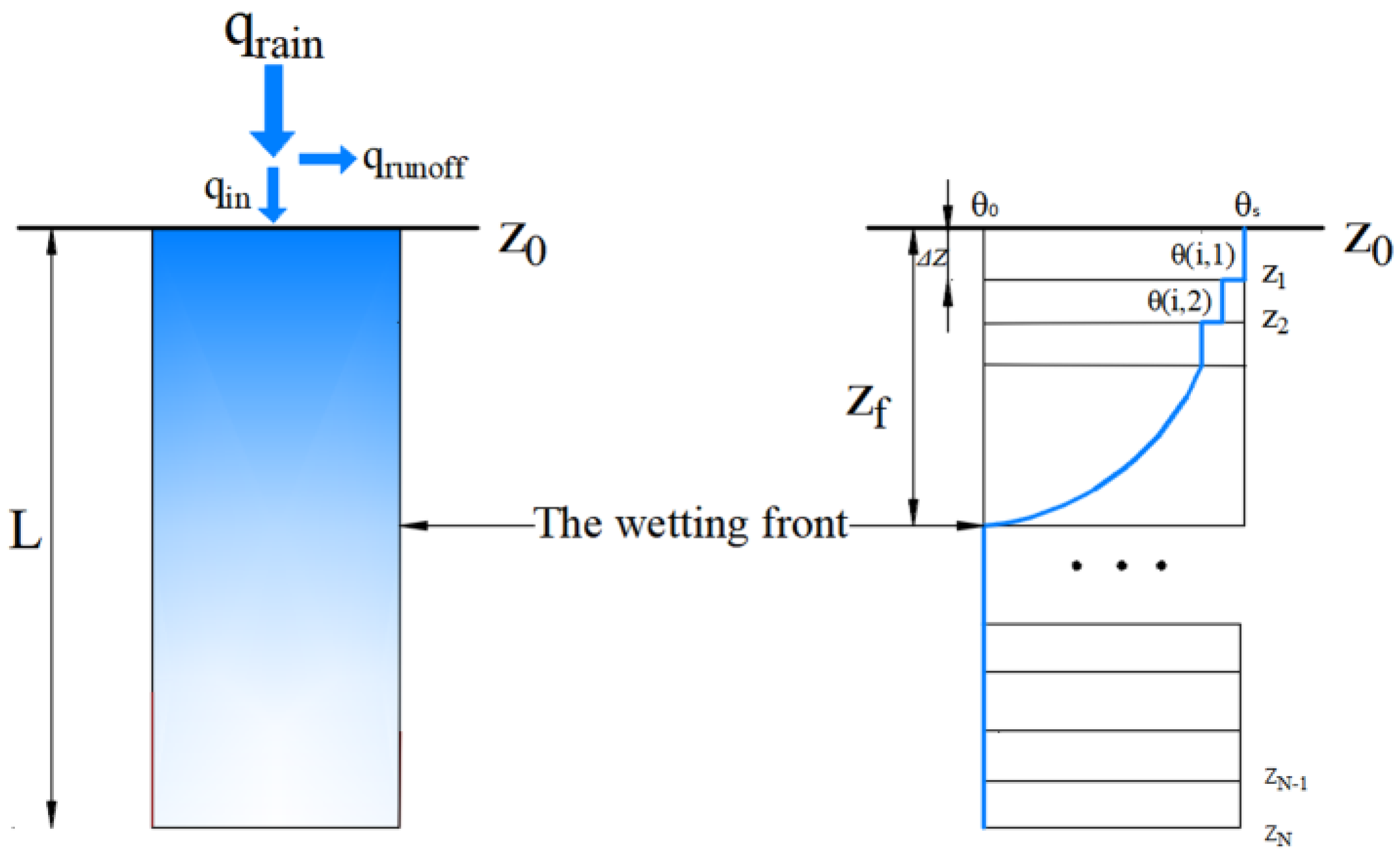
In this paper, the soil model with a free draining condition at the bottom end $z=L$ is discretized, as shown in Figure 1. $L$ is the length of the soil column from the domain top to the bottom. The soil profile in the vertical direction consists of $N$ slices, with the thickness of each slice being $\Delta z$. The depth of the wetting front is $z_f$. The location of the upper boundary for each slice is represented as $z_j=j\times \Delta z\left(j=0,1,2\dots N\right)$, with $z_0$ and $z_N$ representing the domain top and bottom, respectively. The time-step size is $\Delta t=t^{i+1}-t^i\left(i=0,1,2\dots \right)$.

In the beginning of infiltration, an equality to describe the infiltration rate $q_{in}$ at surface and rainfall intensity $q_{rain}$:

$$q_{rain}\left(t\right)=q_{in}\left(t\right)$$

(14)

The equation is established under $\theta \left(0,t\right)\ll {\theta }_s$ at the upper boundary $z_0$. Assuming that when $t=t^i$, the soil water content at $z_0$ is ${\theta }_{temp}\left(i\right)$. Therefore, ${\theta }_{temp}\left(i\right)$ is the upper boundary of slice 1, with the assumption of instantaneous steady saturation. Correspondingly, the boundary conditions of slice 1 at $t=t^i$ are transformed into:

$$\{\begin{array}{l}\theta \left(0,i\right)={\theta }_{temp}\left(i\right)\\ \theta \left(1,i\right)=\theta \left(1,i-1\right)\end{array}i=1,2,3\dots$$

(15)

${\theta }_s$ and ${\theta }_0$ in Equation (13) are replaced by $\theta \left(0,i\right)$ and $\theta \left(1,i\right)$ respectively. Then, $V$ and $D$ can also be expressed as:

$$V_0^i=\frac{K_0^i-K_1^{i-1}}{{\theta }_0^i-{\theta }_1^{i-1}}$$

(16)

$$D_0^i=-\frac{h_s}{\lambda \left({\theta }_s-{\theta }_r\right)}{\left({S_e}_0^i\right)}^{-1/\lambda -1}{K}_0^i$$

(17)

where $K_j^i=K\left({\theta }_j^i\right)$; ${S_e}_j^i=\frac{{\theta }_j^i-{\theta }_r}{{\theta }_s-{\theta }_r}$.

Therefore, the governing equation Equation (13) to obtain $\theta \left(1,i\right)$ can be transformed into:

$${\theta }_1^i={\theta }_1^{i-1}+\frac{{\theta }_0^i-{\theta }_1^{i-1}}{2}\left[erfc\left({F_f}_0^i-{F_s}_0^i\right)+e^{{F_t}_0^i}erfc\left({F_f}_0^i+{F_s}_0^i\right)\right]$$

(18)

where ${F_f}_j^i=\frac{z_{j+1}}{2\sqrt{D_j^i{t}^i}}$; ${F_s}_j^i=\frac{V_j^i{t}^i}{2\sqrt{D_j^i{t}^i}}$; ${F_t}_j^i=\frac{V_j^i{z}_{j+1}}{D_j^i}$.

The infiltration capacity of soil gradually decreases with the time. In this model, the soil infiltration capacity rate $f_P$ and $q_{in}$ can be expressed as:

$$\{\begin{array}{l}{f}_p\left(t^i\right)=-D_0^i\frac{{\theta }_s-{\theta }_0^{i-1}}{dz}+K_s\\ q_{in}\left(t^i\right)=-D_0^j\frac{{\theta }_0^i-{\theta }_1^{i-1}}{dz}+K_0^i\end{array}$$

(19)

When the wetting front reaches to slice $j\left(2\le j\le N\right)$, the boundary conditions are correspondingly expressed as:

$$\{\begin{array}{l}\theta \left(j-1,i\right)={\theta }_{j-1}^i\\ \theta \left(j,i\right)={\theta }_j^{i-1}\end{array},i=1,2\dots j=1,2\dots$$

(20)

The spatial and temporal distribution of soil water content for slice $j$ is:

$${\theta }_j^i={\theta }_j^{i-1}+\frac{{\theta }_{j-1}^i-{\theta }_j^{i-1}}{2}\left[erfc\left({F_f}_{j-1}^i-{F_s}_{j-1}^i\right)+e^{{F_t}_{j-1}^i}erfc\left({F_f}_{j-1}^i+{F_s}_{j-1}^i\right)\right]$$

(21)

Now, $f_P$ and $q_{in}$ can be devised as:

$$\{\begin{array}{l}{f}_p\left(t^i\right)=-D_j^i\frac{{\theta }_s-{\theta }_0^{i-1}}{dz}+K_s\\ q_{in}\left(t^i\right)=-D_j^i\frac{{\theta }_0^i-{\theta }_0^{i-1}}{dz}+K_0^i\end{array}$$

(22)

According to the mass conservation, it is accessible to calculate the increased quantity of moisture per slice. The cumulative infiltration $I$ can be written as:

$$I^i={\displaystyle \sum _{j=0}^N{I}_j^i}={\displaystyle \sum _{j=0}^N\Delta z\left({\theta }_j^i-{\theta }_j^0\right)}$$

(23)

2.2.3. Runoff Calculation

During natural rainfall, the variation of the rainfall intensity is usually a function with respect to time. The distribution and duration of rainfall intensity have an important influence on the soil water content of the soil profile and runoff generation [42]. In general, there are two stages for infiltration under rainfall conditions. Stage 1 is called the rainfall intensity stage. At this stage, the rainfall intensity is less than the infiltration capacity of soils. The surface infiltration rate is equal to the rainfall intensity during stage 1. Stage 2 is called the infiltration capacity control stage. At this stage, the rainfall intensity is greater than the infiltration capacity of soils. The surface infiltration rate is equal to the infiltration capacity of soils. Therefore, the relationship between the infiltration capacity of soils and rainfall intensity determines the different infiltration stages, as shown in the following equation:

$$\{\begin{array}{l}{q}_{rain}\left(t\right)\le f_P\left(t\right)\to q_{in}\left(t\right)=q_{rain}\left(t\right)\\ q_{rain}\left(t\right)>f_P\left(t\right)\to q_{in}\left(t\right)=f_P\left(t\right)\end{array}$$

(24)

The transition time between the two stages is $t_p$. Simultaneously, the surface runoff exists, and the corresponding boundary conditions are:

$$\{\begin{array}{l}\theta \left(0,t_p\right)={\theta }_{i_0}^{i_p}\\ \theta \left(1,t_p\right)={\theta }_1^{i_p}\end{array},i_p=t_p/\Delta t$$

(25)

The runoff rate $q_{runoff}$ can be expressed as:

$$q_{runoff}\left(t_p\right)=q_{rain}\left(t_p\right)-q_{in}\left(t_p\right)$$

(26)

According to the conservation of mass, the relationship between cumulative rainfall $R$ and $I$ is:

$$R^i=I^i+F^i$$

(27)

where $F$ is cumulative runoff.

2.3. Computational Process

We simulated the infiltration process based on a linear analytical solution of the Richards equation. Under different rainfall and initial soil water content conditions, the calculation results show the spatial-temporal distribution of soil water content, the time of runoff, and the cumulative runoff. An automatic judgment of infiltration stages has already been taken to guarantee the preciseness of this computation method. A schematic illustration of the main calculation steps is shown in Figure 2.

3. Results and Discussion

Four types of soils that have quite contrasting hydraulic properties are used for verification and comparison analysis. These hydraulic parameters of four soil types are summarized in

Table 1. The hydraulic parameters of the Brooks–Corey model.

Soil-No.	Soil Type	${\mathit{k}}_{\mathit{s}}\left(\mathbf{cm}/\mathbf{h}\right)$	${\mathit{\theta }}_{\mathit{s}}$	${\mathit{\theta }}_{\mathit{r}}$	$\mathit{\lambda }$	${\mathit{h}}_{\mathit{s}}\left(\mathbf{cm}\right)$	Reference
1	Sand and silt	0.32	0.472	0.041	0.2	−25	Essig et al. [43]
2	Silt sandy loam	1.42	0.477	0.100	1.2	−45	Chu [8]
3	Loamy sand	2.00	0.430	0.008	0.53	−22.6	Nofziger and Wu [22]
4	Loamy soil	0.626	0.404	0.060	0.3	−6.2	Cao and Gong [44]

. In addition, Figure 3 shows the soil–water characteristic curves of the soil types.

3.1. Model Verification

To test the performance of the present solution under steady and unsteady rainfall conditions, the laboratory experimental results and other numerical solutions were utilized to validate the present solution with the same conditions, respectively.

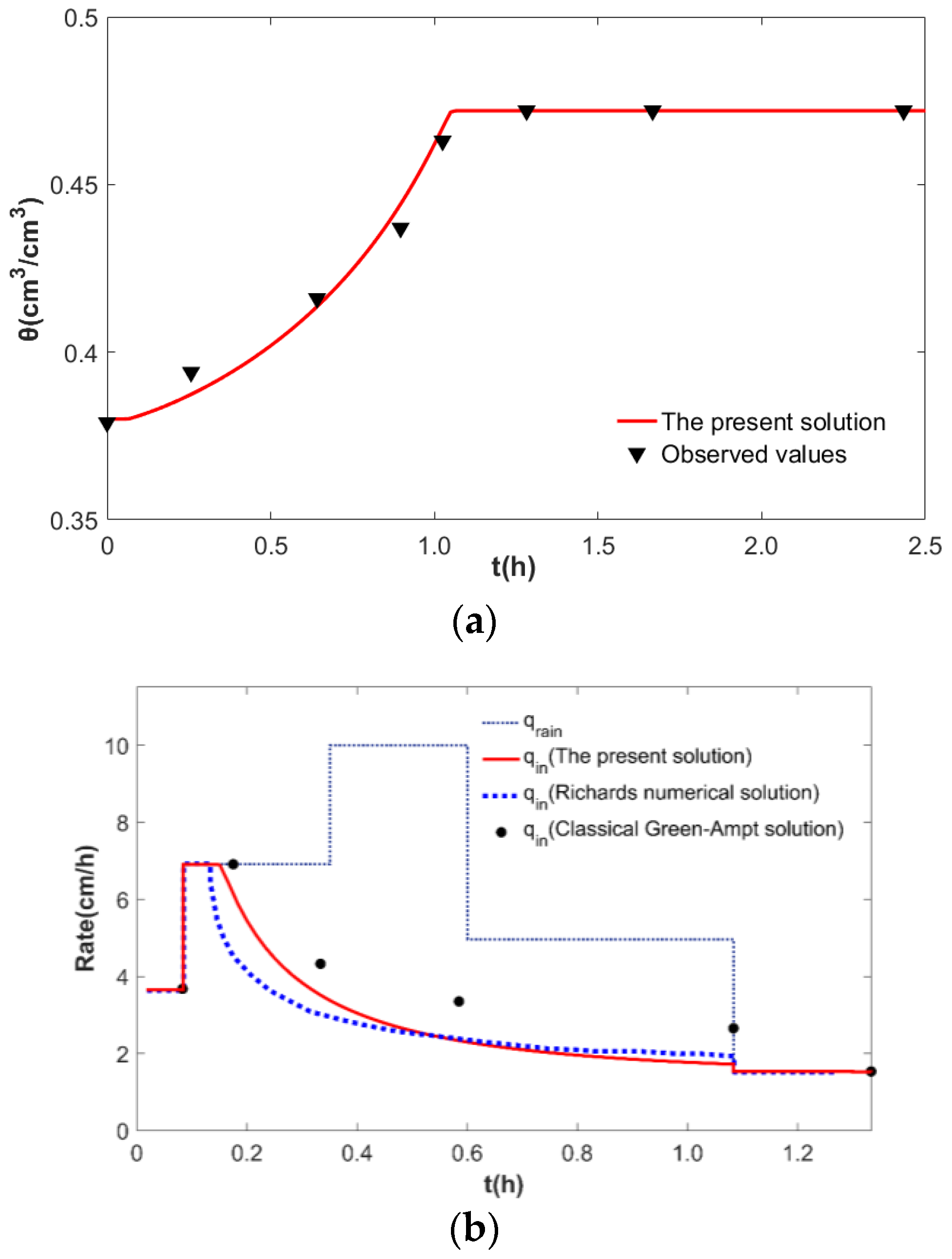
Morbidelli et al. [45] and Essig et al. [43] created a homogeneous soil model with a depth of $L=78\mathrm{cm}$ to observe the experimental phenomena of infiltration and deep flow in the laboratory. Soil-1 is selected in this experiment, and the corresponding hydraulic parameters are shown in Table 1. In addition, the initial soil water content distribution was obtained from Essig et al. [43]. Figure 4a shows the comparison between the present solution and laboratory experimental results under steady rainfall conditions ($q_{rain}=1\mathrm{cm}/\mathrm{h}$). From Figure 4a, the variation of soil water content for the present solution and observed values are similar at a depth of $z=10\mathrm{cm}$. In addition, the time of runoff for the present solution and observed values are 0.317 h and 0.33 h, respectively, and the relative error is 4.0%, indicating that the predictions of water content distribution and time of ponding in the present solution are credible.

Considering a homogeneous soil model with a depth of $L=50\mathrm{cm}$, $\Delta z=0.1\mathrm{cm}$, and $\Delta t=1/60\mathrm{h}$. Soil-2 is selected for this validation, and corresponding hydraulic parameters are reported in Table 1. In addition, the uniform initial soil water content is ${\theta }_0=0.217$. This soil model that was used for verification came from the Richards numerical solution [27] and classical Green–Ampt solution. The classical Green–Ampt method was proposed by Chu and Mariño [9] to simulate the infiltration process through homogeneous soils under unsteady rainfall conditions. The classical Green–Ampt solution was validated by experimental data, and it was credible for the conversion of two infiltration stages under unsteady rainfall conditions.

Figure 4b shows the variations of surface infiltration rate with time under unsteady rainfall conditions. The calculation results show that the present model is available to predict the conversion of two infiltration stages. In Figure 4b, at t = 0.167 h, with the rainfall intensity at 6.91 cm/h, the infiltration stage changes from rainfall intensity to the infiltration capacity control stage, and the runoff exists. When $t=1.083\mathrm{h}$, the rainfall intensity decreases to 1.53 cm/h, which is less than the 1.72 cm/h infiltration capacity of the soil of the present model (the infiltration capacity of soil for the Richards numerical solution and classical Green–Ampt solution are 1.85 cm/h and 2.546 cm/h, respectively). Thus, the infiltration process is at the rainfall intensity stage again.

Table 2. Comparison of calculation results under unsteady rainfall intensity.

Solutions	Cumulative Infiltration	Time of Runoff	Duration of Rainfall Intensity Stage
The present solution	3.74 cm	0.167 h/1.083 h	0.933 h
Richards numerical solution	3.51 cm	0.120 h/1.083 h	0.963 h
Classical Green–Ampt solution	4.54 cm	0.174 h/1.083 h	0.909 h

is a comparison between the above two models and our model. The prediction of $t_p$ in our present solution is closer to the results of classical Green–Ampt solution.

3.2. Comparison Analysis of Different Initial Soil Water Contents

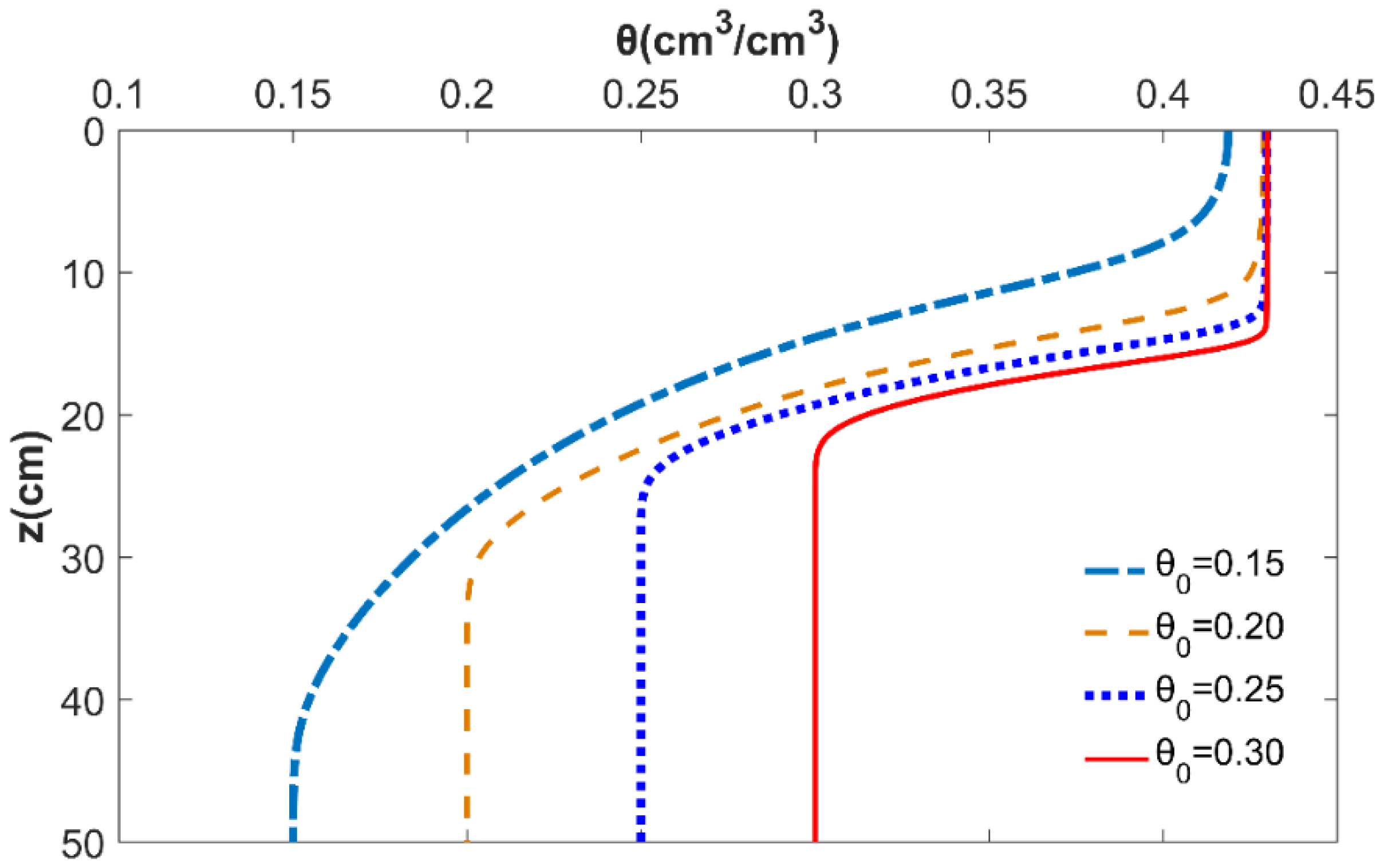
Figure 5 shows the distribution of soil water content after infiltration of 1 h with different initial soil water contents (${\theta }_0=0.15,0.20,0.25,0.30$) under steady rainfall condition $q_{rain}=4\mathrm{cm}/\mathrm{h}$. Soil-3 was adopted in this case, and the hydraulic parameters are also shown in Table 1.

Figure 5 shows that with an increase in the initial soil water content, the depth of the wetting front will decrease ($z_{f1,2,3,4}=49.4\mathrm{cm},35.7\mathrm{cm},28.4\mathrm{cm},25.0\mathrm{cm}$). The successive decreases of the wetting front depth among four initial soil water contents are 27.7%, 20.4%, and 12.0%, respectively. In addition, when the initial soil water content increases, the variation of the soil water content along with the profile will become more acute. The reason is that an increase in the initial soil water content leads to the decrease of the pressure head gradient in the soil profile, resulting in the slower migration rate of infiltrated water through soils.

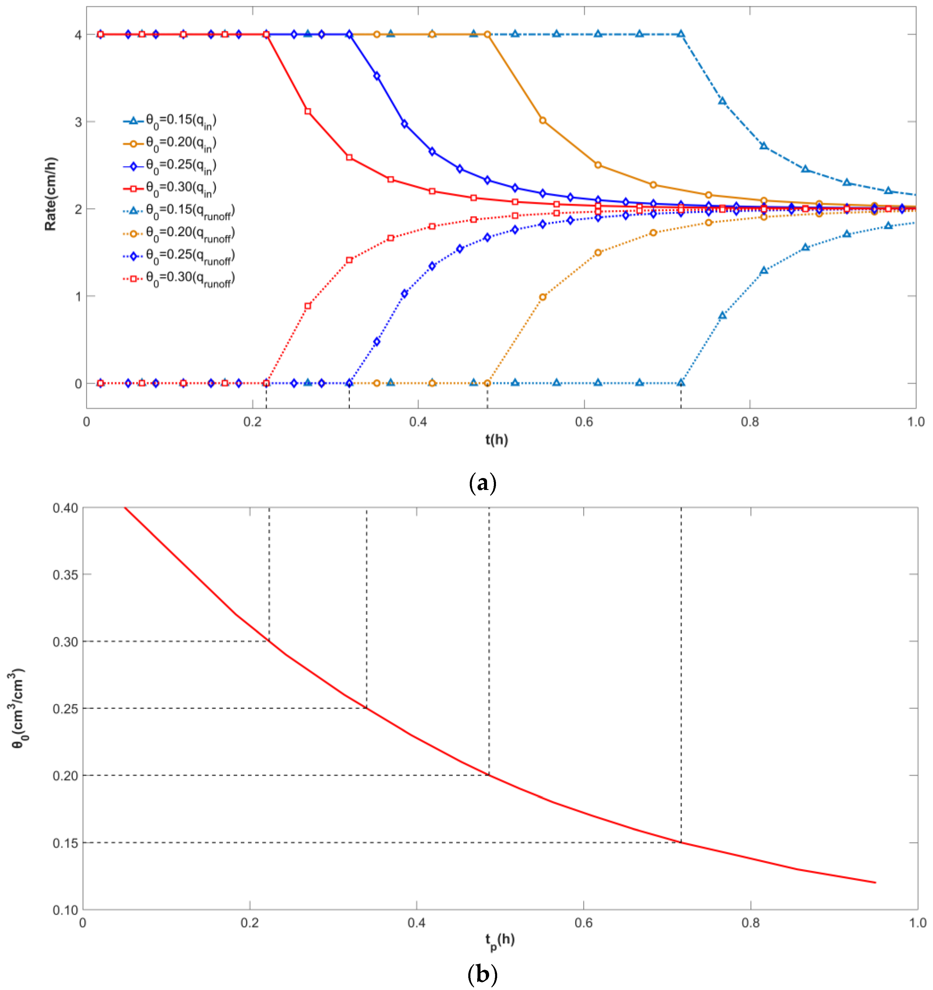
Figure 6a shows the surface infiltration rate and runoff rate with four different initial soil water contents. From Figure 6a, with the increase of initial soil water content, the inflection point of the rate curve will exist in advance, that is, the time of runoff decreases ($t_{p1,2,3,4}=0.717\mathrm{h},0.487\mathrm{h},0.340\mathrm{h},0.223\mathrm{h}$). Figure 6b shows the variation of time of runoff with various initial soil water contents. This result is because the surface soil will be saturated more easily with an increase in the initial soil water content. In addition, the infiltrated water migration rate becomes lower because of the smaller pressure head gradient, leading to a more rapid decrease in the infiltration capacity of the soils.

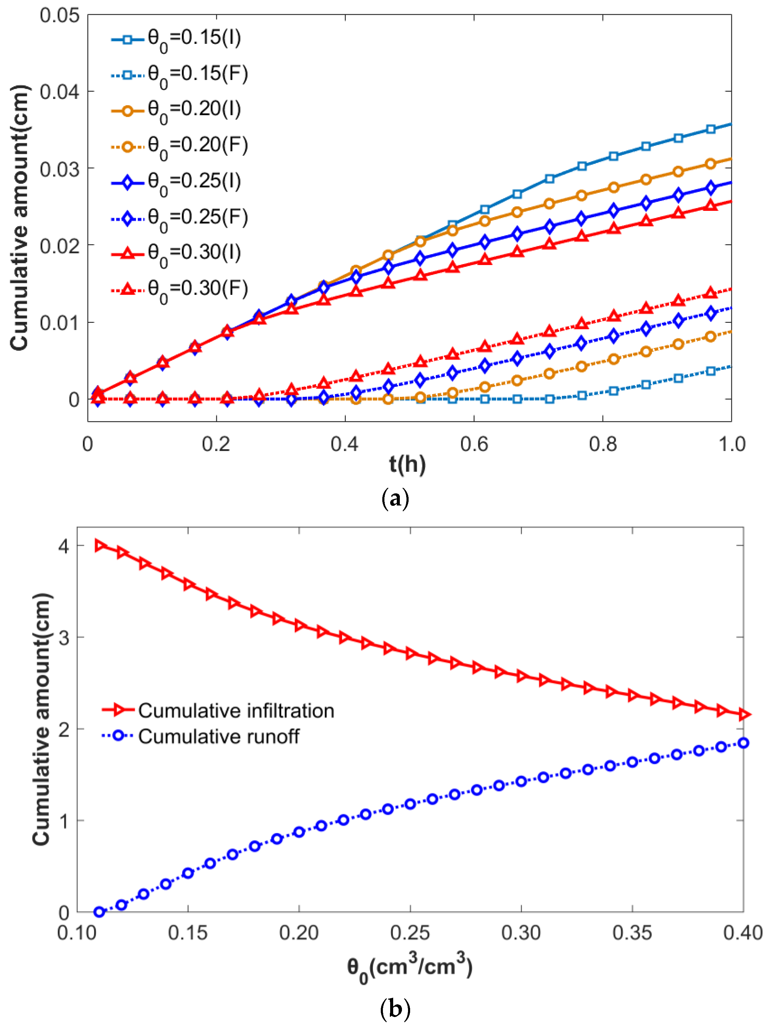
Figure 7a shows the variation of cumulative infiltration and runoff with different initial soil water contents. The cumulative runoff of four different initial soil water contents (${\theta }_0=0.15,0.20,0.25,0.30$) were 0.427 cm, 0.878 cm, 1.185 cm, and 1.431 cm, respectively. The increases of cumulative runoff among the four initial soil water contents were 105.6%, 177.5%, and 235.1% compared with ${\theta }_0=0.15$, respectively. Therefore, the greater the initial soil water content, the slower the cumulative runoff will increase. Figure 7b shows the variation of cumulative infiltration and runoff with different initial soil water contents after an infiltration of 1 h. The results show that with same average rainfall magnitude, the initial soil water content has great influence on the infiltration process. As the initial soil water content increases, the difference in the cumulative infiltration decreases. This is because a larger initial soil water content will lead to a smaller infiltration capacity of soils, and the time of runoff will be shorter. Correspondingly, the cumulative infiltration decreases faster, and the increment of cumulative runoff is larger.

3.3. Comparison Analysis under Different Rainfall Conditions

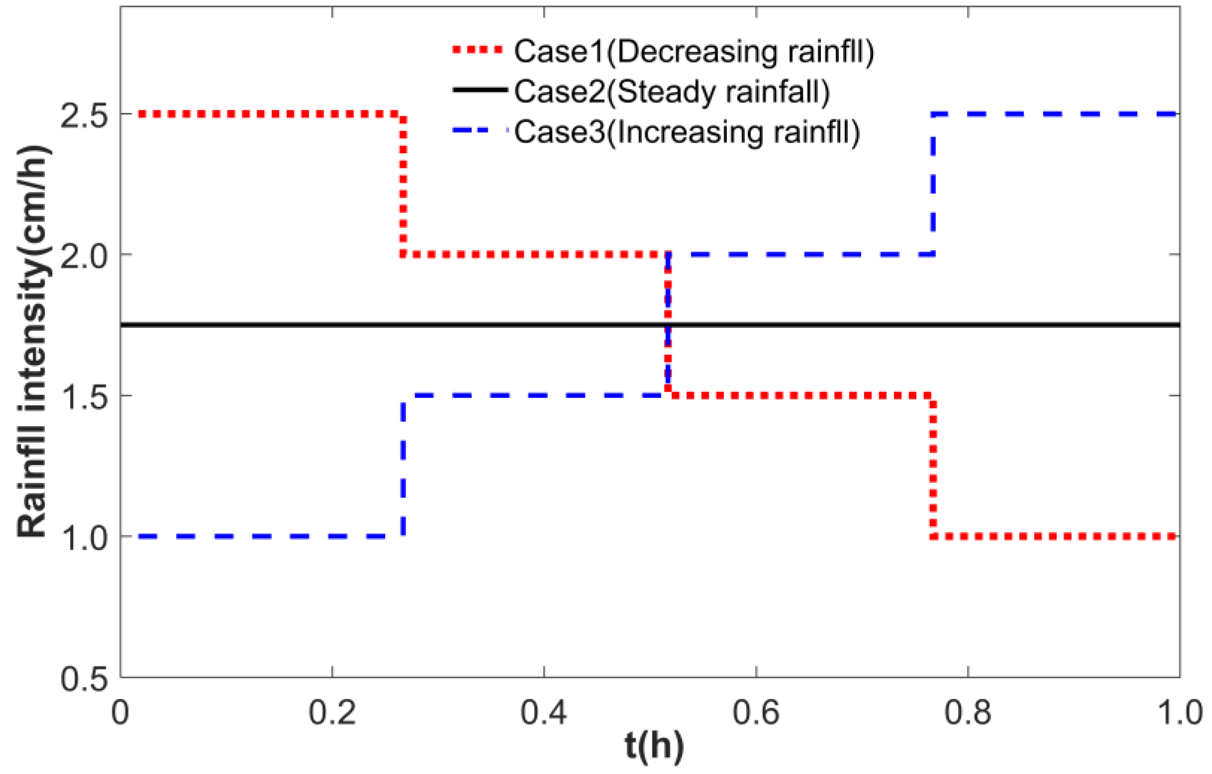
The significant way to control urban flood is a reduction of surface runoff. In this paper, the effect of rainfall conditions on surface runoff was analyzed. The soil sample is Soil-4, with the parameters from Table 1. The rainfall conditions in this paper are classified into rainfall decrease (Case 1), steady rainfall intensity (Case 2), and rainfall increase (Case 3), with the same average magnitude as shown in Figure 8. Figure 9 shows the variations of surface infiltration rate with time under three different rainfall conditions. From Figure 9, the time of runoff with Case 1, Case 2, and Case 3 are 0.450 h, 0.583 h, and 0.667 h, respectively. The runoff with rainfall decrease exists earliest, which is 22.8% and 48.2% earlier than that of Case 2 and Case 3, respectively. The results show that with large rainfall intensity at the initial stage, the surface soil water content increases rapidly, and the pressure head gradient decreases promptly. Correspondingly, the infiltration capacity of soils decreases fast, leading to the early existence of runoff.

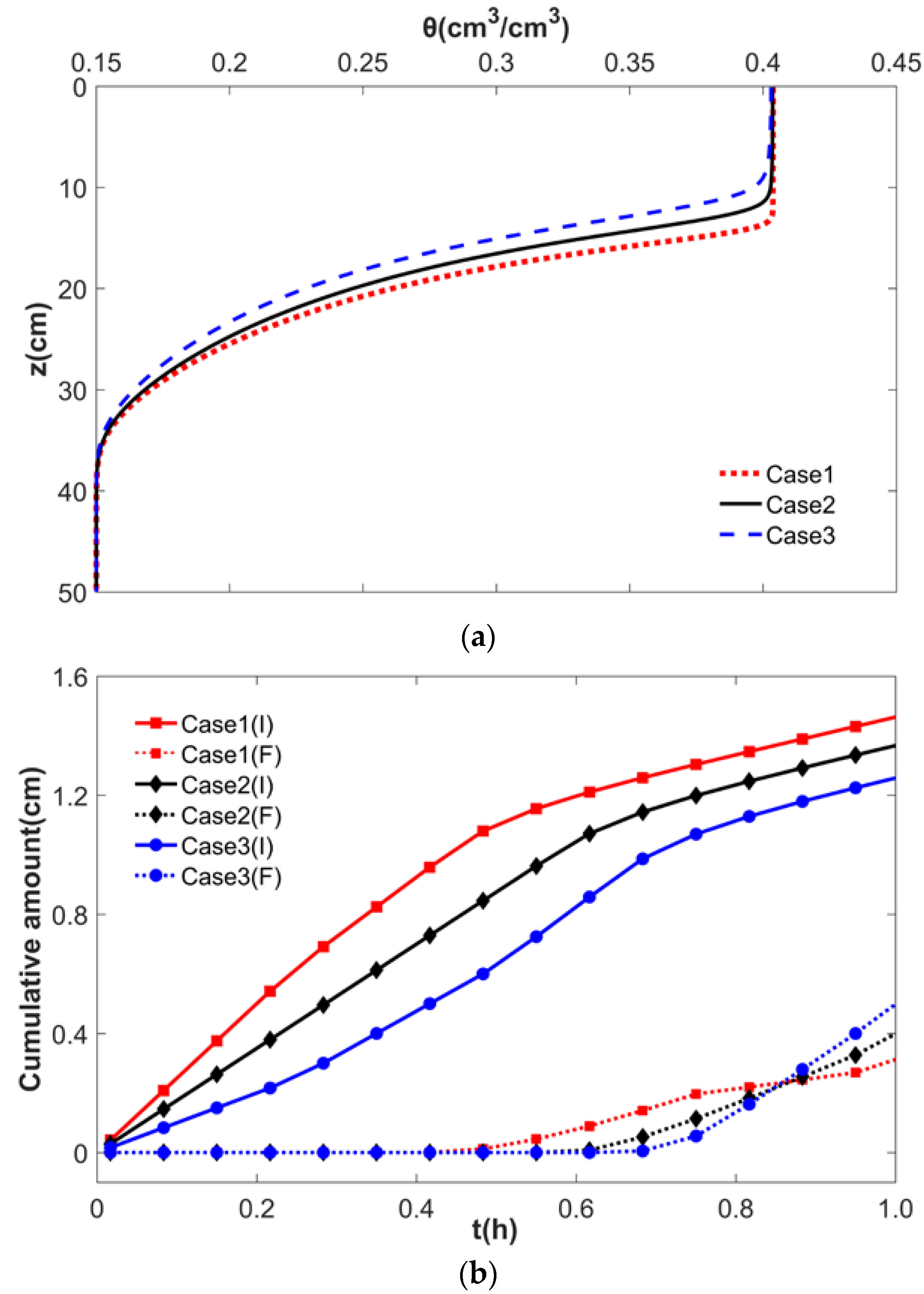
Figure 10a shows the distribution of the soil water content on profile after 1 h of infiltration under three different rainfall conditions. From Figure 10a, the depth of the wetting front under three cases of rainfall intensity were similar ($z_{f1,2,3,4}=40.9\mathrm{cm},41.3\mathrm{cm},41.5\mathrm{cm}$). Furthermore, in same depth, the value of soil water content with decreasing rainfall intensity was greatest among the three cases, while the corresponding value with increasing rainfall intensity was smallest. For Case 1, with a large rainfall intensity at the initial stage, the soil water content increased more in the same depth, which indicates that its cumulative infiltration was largest among the three cases.

Figure 10b shows the variations of cumulative infiltration and runoff under three different rainfall conditions. From Figure 10b, the amounts of cumulative runoff under three cases of rainfall intensity were $F_{1,2,3}=0.287\mathrm{cm},0.383\mathrm{cm},0.492\mathrm{cm}$. Compared with Case 1 and Case 2, the increments of cumulative runoff for Case 3 were 71.2% and 28.4%, respectively. The calculation results showed that the rainfall intensity had a significant influence on infiltration and runoff. With same average rainfall magnitude, among the three cases, the rainfall intensity for Case 3 was the smallest at the initial stage, leading to the slowest increase of soil water content. Correspondingly, the cumulative infiltration of Case 3 increased slower than the other cases. When runoff existed, the rainfall intensity for Case 3 was much greater than the infiltration capacity of soils, so the cumulative runoff increased sharply. Therefore, in the region where increasing rainfall frequently occurred, the vegetation coverage rate should be improved to absorb rainwater. In addition, more reasonable drainage facilities should be utilized to improve the ability of urban rainfall management.

4. Conclusions

It’s significant to model infiltration into soil and understand the corresponding characteristics for flooding management, agriculture, and environmental protection. A flow model through unsaturated soils was established combining a conventional analytical solution with a numerical approach. The calculation approach of soil water content and runoff prediction under unsteady rainfall condition was presented. The calculation results of soil water content versus time in terms of the present solution have good agreements with the experimental results. In addition, the present solution was also important for the verification of numerical schemes and the classical Green–Ampt solution as well as for checking the implementation of the prediction ponding time.

The calculation results indicated that the cumulative infiltration with decreasing rainfall is highest among the three conditions under same average magnitude. The cumulative runoff is smaller than the decreasing rainfall at the initial stage, and then becomes larger at the later stage. This is due to the soil water content increasing, and the infiltration capacity decreasing faster with the increasing rainfall at the initial stage, and then decreasing rainfall on the contrary at the later stage.

The time of runoff with decreasing rainfall (Case 1) is earliest among the three rainfall conditions, which is about 50% earlier than the increasing rainfall (Case 3). The time of the runoff would shorten by roughly 70% once the initial soil water content doubles from 0.15 to 0.3 in a loamy sand. The results provide theoretical fundamentals to monitor surface runoff and defend urban flood under different rainfall conditions. This novel approach can be utilized easily and effectively for modeling infiltration and runoff evaluation.

References

- Dunne, T.; Leopold, L.B. Water in Environment Planning; W. H. Freeman: London, UK, 1978; Volume 44, p. 502. [Google Scholar]
- Morbidelli, R.; Saltalippi, C.; Flammini, A.; Cifrodelli, M.; Corradini, C.; Govindaraju, R.S. Infiltration on sloping surfaces: Laboratory experimental evidence and implications for infiltration modeling. J. Hydrol. 2015, 523, 79–85. [Google Scholar] [CrossRef]
- Lai, W.; Ogden, F.L. A mass-conservative finite volume predictor–corrector solution of the 1D Richards’ equation. J. Hydrol. 2015, 523, 119–127. [Google Scholar] [CrossRef]
- Ahmadaali, J.; Barani, G.-A.; Qaderi, K.; Hessari, B. Analysis of the effects of water management strategies and climate change on the environmental and agricultural sustainability of Urmia Lake Basin, Iran. Water 2018, 10, 160. [Google Scholar] [CrossRef]
- Green, W.H.; Ampt, G.A. Studies on soil phyics, part 1. The flow of air and water through soils. J. Agric. Sci. 1911, 4, 11–24. [Google Scholar]
- Richards, L.A. Capillary conduction of liquids through porous mediums. Physics 1931, 1, 318–333. [Google Scholar] [CrossRef]
- Mein, R.G.; Larson, C.L. Modeling infiltration during a steady rain. Water Resour. Res. 1973, 9, 384–394. [Google Scholar] [CrossRef]
- Chu, S.T. Infiltration during an unsteady rain. Water Resour. Res. 1978, 14, 461–466. [Google Scholar] [CrossRef]
- Chu, X.; Mariño, M.A. Determination of ponding condition and infiltration into layered soils under unsteady rainfall. J. Hydrol. 2005, 313, 195–207. [Google Scholar] [CrossRef]
- Craig, J.R.; Liu, G.; Soulis, E.D. Runoff-infiltration partitioning using an upscaled Green-Ampt solution. Hydrol. Process. 2010, 24, 2328–2334. [Google Scholar] [CrossRef]
- Corradini, C.; Flammini, A.; Morbidelli, R.; Govindaraju, R.S. A conceptual model for infiltration in two-layered soils with a more permeable upper layer: From local to field scale. J. Hydrol. 2011, 410, 62–72. [Google Scholar] [CrossRef]
- Corradini, C.; Morbidelli, R.; Flammini, A.; Govindaraju, R.S. A parameterized model for local infiltration in two-layered soils with a more permeable upper layer. J. Hydrol. 2011, 396, 221–232. [Google Scholar] [CrossRef]
- Zhu, J. Effect of Layered Structure on Anisotropy of Unsaturated Soils. Soil Sci. 2012, 177, 139–146. [Google Scholar] [CrossRef]
- Deng, P.; Zhu, J. Analysis of effective Green–Ampt hydraulic parameters for vertically layered soils. J. Hydrol. 2016, 538, 705–712. [Google Scholar] [CrossRef]
- Hsu, S.-Y.; Huang, V.; Woo Park, S.; Hilpert, M. Water infiltration into prewetted porous media: Dynamic capillary pressure and Green-Ampt modeling. Adv. Water Resour. 2017, 106, 60–67. [Google Scholar] [CrossRef]
- Nie, W.-B.; Li, Y.-B.; Fei, L.-J.; Ma, X.-Y. Approximate explicit solution to the green-ampt infiltration model for estimating wetting front depth. Water 2017, 9, 609. [Google Scholar] [CrossRef]
- Neuman, S.P. Saturated-unsaturated seepage by finite elements. J. Hydraul. Div. 1973, 99, 2233–2250. [Google Scholar]
- Pullan, A.J.; Collins, I.F. Two- and three-dimensional steady quasi-linear infiltration from buried and surface cavities using boundary element techniques. Water Resour. Res. 1987, 23, 1633–1644. [Google Scholar] [CrossRef]
- Clement, T.P.; William, R.W.; Fred, J.M. A physically based, two-dimensional, finite-difference algorithm for modeling variably saturated flow. J. Hydrol. 1994, 161, 71–90. [Google Scholar] [CrossRef]
- Romano, N.; Brunone, B.; Santini, A. Numerical analysis of one-dimensional unsaturated flow in layered soils. Adv. Water Res. 1998, 21, 315–324. [Google Scholar] [CrossRef]
- Belfort, B.; Younes, A.; Fahs, M.; Lehmann, F. On equivalent hydraulic conductivity for oscillation–free solutions of Richard’s equation. J. Hydrol. 2013, 505, 202–217. [Google Scholar] [CrossRef]
- Nofziger, D.; Wu, J. Chemflo-2000: Interactive Software for Simulating Water and Chemical Movement in Unsaturated Soils; U.S. Environmental Protection Agency: Washington, DC, USA, 2003.
- Wiltshire, R.; Elkafri, M. Non-classical and potential symmetry analysis of Richard’s equation for moisture flow in soil. J. Phys. A Math. Gen. 2004, 37, 823–839. [Google Scholar] [CrossRef]
- Hagare, D.; Sivakumar, M.; Bunsri, T. Numerical modelling of tracer transport in unsaturated porous media. J. Appl. Fluid Mech. 2008, 1, 62–79. [Google Scholar]
- Weill, S.; Mouche, E.; Patin, J. A generalized Richards equation for surface/subsurface flow modelling. J. Hydrol. 2009, 366, 9–20. [Google Scholar] [CrossRef]
- Kavetski, D.; Binning, P.; Sloan, S.W. Adaptive backward Euler time stepping with truncation error control for numerical modelling of unsaturated fluid flow. Int. J. Numer. Methods Eng. 2002, 53, 1301–1322. [Google Scholar] [CrossRef]
- Herrada, M.A.; Gutiérrez-Martin, A.; Montanero, J.M. Modeling infiltration rates in a saturated/unsaturated soil under the free draining condition. J. Hydrol. 2014, 515, 10–15. [Google Scholar] [CrossRef]
- Ghotbi, A.R.; Omidvar, M.; Barari, A. Infiltration in unsaturated soils—An analytical approach. Comput. Geotech. 2011, 38, 777–782. [Google Scholar] [CrossRef]
- Srivastava, R.; Yeh, T.-C.J. Analytical solutions for one-dimensional, transient infiltration toward the water table in homogeneous and layered soils. Water Resour. Res. 1991, 27, 753–762. [Google Scholar] [CrossRef]
- Hayek, M. An analytical model for steady vertical flux through unsaturated soils with special hydraulic properties. J. Hydrol. 2015, 527, 1153–1160. [Google Scholar] [CrossRef]
- Subbaiah, R. A review of models for predicting soil water dynamics during trickle irrigation. Irrig. Sci. 2011, 31, 225–258. [Google Scholar] [CrossRef]
- Tracy, F.T. Using analytic solution methods on unsaturated seepage flow computations. Procedia Comput. Sci. 2016, 80, 554–564. [Google Scholar] [CrossRef]
- Hayek, M. An exact explicit solution for one-dimensional, transient, nonlinear Richards’ equation for modeling infiltration with special hydraulic functions. J. Hydrol. 2016, 535, 662–670. [Google Scholar] [CrossRef]
- Zlotnik, V.A.; Wang, T.; Nieber, J.L.; Šimunek, J. Verification of numerical solutions of the Richards equation using a traveling wave solution. Adv. Water Resour. 2007, 30, 1973–1980. [Google Scholar] [CrossRef]
- Ku, C.-Y.; Liu, C.-Y.; Xiao, J.-E.; Yeih, W. Transient modeling of flow in unsaturated soils using a novel collocation meshless method. Water 2017, 9, 954. [Google Scholar] [CrossRef]
- Chen, J.-M.; Tan, Y.-C.; Chen, C.-H. Analytical solutions of one-dimensional infiltration before and after ponding. Hydrol. Process. 2003, 17, 815–822. [Google Scholar] [CrossRef]
- Mmolawa, K.; Or, D. Experimental and numerical evaluation of analytical volume balance model for soil water dynamics under a drip irrigation. Soil Sci. Soc. Am. J. 2003, 67, 1657–1671. [Google Scholar] [CrossRef]
- Brooks, R.H.; Corey, A.T. Hydraulic Properties of Porous Media; McGill-Queen’s University Press: Kingston, ON, Canada, 1964; pp. 352–366. [Google Scholar]
- Genuchten, M.T.V. A closed-form equation for predicting the hydraulic conductivity of unsaturated soils. Soil Sci. Soc. Am. J 1980, 44, 892–898. [Google Scholar] [CrossRef]
- Menziani, M.; Pugnaghi, S.; Vincenzi, S. Analytical solutions of the linearized Richards equation for discrete arbitrary initial and boundary conditions. J. Hydrol. 2007, 332, 214–225. [Google Scholar] [CrossRef]
- Abramowitr, M.; Stegun, I.A.; Abramowitr, M.; Stegun, I.A. Handbook of Mathematical Functions; Dover Publications, Inc.: New York, NY, USA, 1965; pp. 136–144. [Google Scholar]
- Furman, A. Modeling coupled surface–subsurface flow processes: A review. Vadose Zone J. 2008, 7, 741. [Google Scholar] [CrossRef]
- Essig, E.T.; Corradini, C.; Morbidelli, R.; Govindaraju, R.S. Infiltration and deep flow over sloping surfaces: Comparison of numerical and experimental results. J. Hydrol. 2009, 374, 30–42. [Google Scholar] [CrossRef]
- Cao, Q.; Gong, Y. Simulation and analysis of water balance and nitrogen leaching using Hydrus-1D under winter wheat crop. Plant Nutr. Fertil. Sci. 2003, 9, 139–145. [Google Scholar]
- Morbidelli, R.; Corradini, C.; Saltalippi, C.; Rao, S.G. Laboratory experimental investigation of infiltration by the run-on process. J. Hydrol. Eng. 2008, 13, 1187–1192. [Google Scholar] [CrossRef]
Figure 1.
Spatial discretization of homogeneous soil column.
Figure 2.
Flow chart of computational process.
Figure 3.
Soil–water characteristic curves of different soil types. (a) Pressure head curves; (b) Hydraulic conductivity curves.
Figure 4.
Comparison of surface infiltration rate between the present model and reference models. (a) Validation between the present solution and observed data under steady rainfall intensity; (b) Validations between the present solution and other solutions under unsteady rainfall intensity.
Figure 5.
Profiles of soil water content at with different initial soil water contents.
Figure 6.
Infiltration and runoff versus time with different initial soil water contents. (a) Infiltration and runoff rate with different initial soil water contents; (b) Runoff time versus initial soil water contents.
Figure 7.
Cumulative infiltration and runoff versus time with different initial soil water contents. (a) Cumulative infiltration and cumulative runoff with different initial soil water contents; (b) Cumulative amount versus initial soil water contents at .
Figure 8.
Diagram of three different rainfall intensity conditions.
Figure 9.
Surface infiltration rate under three different rainfall intensity conditions.
Figure 10.
Calculation results with three cases. (a) Profiles of soil water content at ; (b) Cumulative infiltration and cumulative runoff versus time.