Flow Partitioning Modelling Using High-Resolution Isotopic and Electrical Conductivity Data


1
Departamento de Recursos Hídricos y Ciencias Ambientales, Facultad de Ingeniería, Facultad de Ciencias Agropecuarias, Universidad de Cuenca, Cuenca 010111, Ecuador
2
Institute for Landscape Ecology and Resources Management (ILR), Research Centre for BioSystems, Land Use and Nutrition (IFZ), Justus Liebig University Giessen, 35392 Giessen, Germany
3
Department of Forest Engineering, Resources, and Management, Oregon State University, Corvallis, OR 97330, USA
*
Author to whom correspondence should be addressed.
Water 2018, 10(7), 904; https://doi.org/10.3390/w10070904
Submission received: 29 May 2018
/
Revised: 6 July 2018
/
Accepted: 6 July 2018
/
Published: 9 July 2018
(This article belongs to the Section Hydrology)
Abstract
:Water-stable isotopic (WSI) data are widely used in hydrological modelling investigations. However, the long-term monitoring of these tracers at high-temporal resolution (sub-hourly) remains challenging due to technical and financial limitations. Thus, alternative tracers that allow continuous high-frequency monitoring for identifying fast-occurring hydrological processes via numerical simulations are needed. We used a flexible numerical flow-partitioning model (TraSPAN) that simulates tracer mass balance and water flux response to investigate the relative contributions of event (new) and pre-event (old) water fractions to total runoff. We tested four TraSPAN structures that represent different hydrological functioning to simulate storm flow partitioning for an event in a headwater forested temperate catchment in Western, Oregon, USA using four-hour WSI and 0.25-h electrical conductivity (EC) data. Our results showed strong fits of the water flux and tracer signals and a remarkable level of agreement of flow partitioning proportions and overall process-based hydrological understanding when the model was calibrated using either tracer. In both cases, the best model of the rainstorm event indicated that the proportion of effective precipitation routed as event water varies over time and that water is stored and routed through two reservoir pairs for event and pre-event. Our results provide great promise for the use of sub-hourly monitored EC as an alternative tracer to WSI in hydrological modelling applications that require long-term high-resolution data to investigate non-stationarities in hydrological systems.
1. Introduction
The identification of the water sources contributing to runoff is fundamental to understand the linkage and interactions between water and biogeochemical cycles and the transport of contaminants and solutes at the catchment and landscape scales [1,2,3,4]. During precipitation events total runoff can be partitioned into event—“new” water from incoming precipitation—and pre-event water—“old” water stored in the catchment prior to a given precipitation event [5,6]. Depending on the catchment conditions (e.g., vegetation, soil type, geology, topography, antecedent moisture) and event characteristics (e.g., precipitation amount and temporal variability) the event and pre-event water fractions vary. As such, understanding the spatial and temporal variability of the contributions of different water pools to the hydrograph is not only a fundamental question in hydrological science [7], but is also needed for the implementation of effective water resources management strategies worldwide [8].
Given that the contribution of different water pools to total runoff is time dependent owing to the time variant nature of flow response processes [7,9,10,11,12], we struggle to apply effective monitoring strategies in catchments with different environmental conditions [13]. Conservative (e.g., water stable isotopes, 2H and 18O, and chloride) and non-conservative (e.g., electrical conductivity (EC) and silica) tracers have been used to constrain mixing models of flow partitioning at the event scale (e.g., [14,15,16,17,18]). One of the most commonly applied methods is tracer-based two-component end member mixing analysis [5,6,19,20] to quantify the proportions of event and pre-event water to total runoff using a simple mass balance (cf., Buttle [5] and Klaus and Mcdonnell [6] for reviews). However, since these models only account for the mixing of the tracer within a hydrological system, they provide only limited information about the combined flow and tracer mixing dynamics in response to precipitation inputs. Therefore, these models have limited ability to provide a process-based understanding of catchment behavior [21,22,23].
In response to this challenge, numerical models in which the tracer mass balance and the hydrological flow response are coupled have been developed [24,25,26,27]. These models allow for the simultaneous simulation of the streamflow hydrograph—water flux—and the tracer mixing. In general, these models account for the water flux partitioning by applying the unit hydrograph approach, and the tracer mixing using travel time distributions (TTDs) [28]. The application of TTDs accounts for the estimation of the possible travel times of the tracer within the system. That is, the time that a water molecule takes to travel within a hydrological system from the moment it enters as precipitation or snowmelt to the time it exists as runoff [29,30]. The TTDs shapes are used to identify runoff processes [7,29,31,32] by providing information about the physical processes that influence the internal mixing of different water sources.
Despite the advantages of numerical approaches for hydrograph separation, the availability of long-term high-resolution water geochemical data remains a challenge. To date, the majority of applications of tracer-based hydrograph separation techniques have been conducted using WSIs as tracers [6]. Despite their recognized usefulness and reliability (being conservative), WSIs sampling at fine resolution (e.g., sub-hourly) is still sparse given high associated costs and, thus, limits the description of the rapid response of streamflow to water inputs and the inter-storm variation of the input isotopic composition [33,34,35,36]. This limitation has resulted in high uncertainties in the estimation of flow components [35,37]. Recent studies have monitored WSIs at high-temporal resolution (every 30 min) [38,39,40,41,42,43] and applied simple mixing models to partition flow components [9,18,44,45]. However, while technological developments currently allow the deployment of field analyzers to measure the WSI of inputs and outputs (e.g., rainfall and streamflow) at high temporal resolution it is unfeasible to broadly implement such analyzers. Thus, there is a need for alternative inexpensive and low maintenance water quality parameters (i.e., tracers) that allow investigating internal catchment processes at a high resolution [13,46].
Electrical conductivity, or specific conductance (EC) of water, is an alternative tracer often used in flow partitioning and water quality studies, either alone or in combination with WSIs (e.g., [16,20,47,48,49,50,51,52,53,54]). The main advantage of using EC is that it can be continuously monitored at high temporal resolution (seconds to minutes) using inexpensive in-stream probes [13,46,48]. Despite the non-conservative nature of EC as it highly depends on the water contact time with the mineral substrate, in particular [53,55,56], EC has yielded similar streamflow portioning results than WSIs using traditional mass balance models [16,51]. However, its effectiveness has not been tested against WSI using sophisticated hydrological modeling approaches.
In this study, we compare the results of a flow partitioning tracer-based hydrological model calibrated using WSIs and EC. Our specific objectives are: (1) to evaluate different model structures (representing different assumptions of the internal catchment hydrological functioning) and determine the model structure that best simulates flow partitioning using WSI and EC data; and (2) to compare the process-based hydrological understanding obtained from the models calibrated using each tracer.
2. Materials and Methods
2.1. Study Area
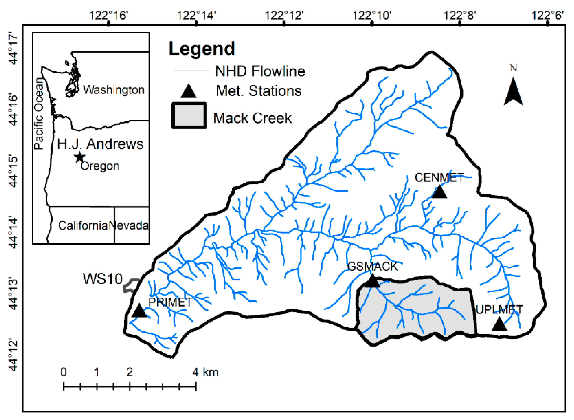
This study was conducted at the Mack Creek catchment (5.8 km2) in the H.J. Andrews Experimental Forest in the Western Cascades of Oregon (Figure 1). Mack Creek is a tributary of Lookout Creek, which drains into the Blue and McKenzie rivers within the Willamette River Basin. Glaciation occurred in the catchment leaving U-shaped valley morphologies with a steep slope (average 46%). The elevation ranges between 758 and 1610 m above sea level (a.s.l.) [57,58]. The catchment is underlie by ridge-capping andesite lava flows (upper Sardine Formation and Pliocene flows). The soils in the catchment are gravelly loams at high elevation that transition into the predominantly gravelly sandy loams that characterize over 70% of Mack Creek drainage area [59]. The forest is dominated by 400–500 year-old coniferous trees, including Douglas fir (Psuedotsuga menziesii), western hemlock (Tsuga heterophylla), and western red cedar (Thuja plicata). The climate is Mediterranean with wet, mild winters and dry summers. Fall and winter precipitation falls as a mix of rain and snow and may accumulate and last from early November to late June [60]. Mean annual precipitation (between 2002 and 2016) was 2243 and 2709 mm at the CENMET (1018 m a.s.l.) and UPMET (1294 m a.s.l.) meteorological stations (Figure 1), respectively. However, precipitation in 2015—when we conducted this study—was only 51% of this 15-year average and fell almost entirely in the form of rain.
2.2. Hydrometric Data Collection
We monitored water fluxes—precipitation (P) and streamflow (Q)—during a large rainstorm event between 28 October and 7 November 2015. We used 5-min resolution P and Q data maintained as part of the NSF Long-Term Ecological Research (LTER) program [61]. We used Q data derived from an 18-in flume (GSMACK; Figure 1) [61] and mean P values across the UPMET station and a precipitation tipping bucket located in the roof top of the GSMACK [62]. The 8-in diameter GSMACK gauge is heated with a propane heater. Continuous precipitation is recorded with depth measurements using a Stevens A-35 chart recorder or a Stevens PAT water level shaft encoder. The UPMET precipitation gauge is stand-alone composed of standing pipe with tank gauge, a propane-heated 20-inch diameter orifice, surrounded by a Valdai-style double wind fence. A temperature probe controls the orifice heating by turning a pump and heater on/off. The stand-alone rain gauge was specifically developed to withstand heavy snow with depths up to 3–4 m and windy condition.
2.3. Water Stable Isotope Data Collection and Analysis
We collected 44,500 mL streamflow grab samples every 4 h using an automatic autosampler (ISCO-3700). A grab sample was also collected before the event in order to characterize the streamflow isotopic composition during base flow conditions (i.e., pre-event). We described the event isotopic signature of precipitation at a meteorological station located at 430 m a.s.l. (PRIMET; Figure 1) with a sequential rainfall sampler designed to collect up to 12,200-mL water samples to characterize the temporal variability of water stable isotopes [33,63]. The sequential collector was located in a clearing, thus, we assumed that the difference between the isotopic signature of direct rainfall and throughfall was minimal [64]. All water samples for isotopic analysis were collected and stored in 20-mL glass bottles with conical inserts without headspace and kept in dark at relatively cool conditions (~15 °C) to avoid fractionation by evaporation until their analysis was conducted at the Watershed Processes Laboratory at Oregon State University.
We measured the water-stable isotopes (δ18O) in all samples using a cavity ring down spectroscopy liquid and vapor isotopic analyzer (Picarro L2130-i, Picarro Inc, Santa Clara, CA). We ran all samples under high-precision, including six injections per sample. The first three injections were discarded to account for memory effects. Two internal (secondary) standards (MET1, δ18O = −14.49‰ and BB1, δ18O = −7.61‰) were used to develop calibration curves, while a third internal standard (ALASKA1, δ18O = −11.09‰) was used to estimate a drift correction equation (drift was always below 0.000152‰). All internal standards were calibrated against the IAEA primary standards for the Vienna Standard Mean Ocean Water (VSMOW2, δ18O = 0.0‰), Greenland Ice Sheet Precipitation (GISP, δ18O = −24.76‰), and Standard Light Antarctic Precipitation (SLAP2, δ18O = −55.5‰). The uncertainty in our secondary standards (i.e., standard deviation) is <0.01‰. Based on >50 duplicate samples (collected concurrently under comparable conditions) in rainfall and streamflow, we estimated an internal laboratory precision of 0.03‰. The external accuracy of our laboratory was 0.06‰. This accuracy was computed as the mean difference between 60 estimated values and a known water standard. We used only the internal precision as an overall measure of accuracy although we acknowledge that there are other sources of uncertainty [65].
2.4. Electrical Conductivity Measurements
We measured the conductance of the sequential water samples collected for the water stable isotopes analysis using a Hanna® Multiparameter (HI9828) Water Quality Portable Meter and used these measurements to characterize the EC of the precipitation during the event. The portable meter was calibrated in the laboratory following manufacture guidelines. The manufacture accuracy of this instrument is 1% or 1 μS/cm (whichever is larger). Replicate measurements for 30 samples indicated a precision of <5%. The EC measurements were conducted after the 20-mL samples for water stable isotopes were collected to avoid sample contamination. Streamflow EC was continuously recorded (every 5 min) at the GSMACK gauge with a Campbell Scientific CS547A EC and temperature probe (with a 5% accuracy) [66]. The EC data is corrected with a temperature coefficient based on YSI Pro30 conductivity instrument [66].
2.5. Tracer-Based Hydrograph Separation Modeling
In recent years, different approaches that allow the incorporation of geochemical tracers mixing into hydrological models have been developed. The application of conceptual models using TTD functions [25,27,67] and ranked storage-age-selection (rSAS) functions [68] are amongst the most frequently applied approaches. We selected the former approach as it allows for the implementation of different model structures (representing different catchment hydrological behavior) that have been widely tested using WSI for model calibration in other studies and, thus, allow for a direct comparison with our results using both high-resolution WSIs and EC data.
We used the flexible modelling framework developed by Segura et al. [25] that considers both the tracer mass balance and the hydrological flow response during rainfall-runoff events. We refer to this model as TraSPAN (Tracer-based Streamflow Partitioning ANalysis model). TraSPAN shares similarities with other tracer-based hydrological models (e.g., [24,27]). It allows for the implementation of different model structures to simulate different levels of hydrological complexity, assuming that rainfall-runoff can be partitioned into event and pre-event components. As such, we implemented this framework to evaluate competing hypotheses of hydrological response against observed Q and tracer data to select the best model structure for the given hydrological system [26,69,70].
TRaSPAN is composed of three modules (Table 1). Module 1: The effective rainfall module is a non-linear routine that computes the effective rainfall (Peff) as the product of precipitation (P) and the antecedent rainfall index (s) [71] (Equations (1) and (2) in Table 1). Module 2: The event and pre-event routing module defines the fraction Peff routed as either event or pre-event water. Module 3: The Event and pre-event transfer functions module includes the TTDs to convolve the fractions of event and pre-event water and, thus, represents the internal hydrological behavior of the system. Modules 2 and 3 are flexible, allowing for the fraction (f) of Peff routed as event water to be constant or time-variant (i.e., to vary over the duration of the event; Equation (3) in Table 1) and for the incorporation of TTDs of varying degrees of complexity into the convolution integrals for event ant pre-event water (Equations (4) and (5)). Even though there exists a variety of theoretical TTDs that could represent tracer mixing in hydrological models, we selected two of the most commonly applied TTDs that have been tested to represent hydrological systems in other catchments [27,72,73]. These are the exponential model (EM; [74]) representing a single linear reservoir (Equations (6) and (7) in Table 1) and the two-parallel linear reservoirs model (TPLR; [27]) representing two connected linear reservoirs (Equations (9) and (10) in Table 1). A detailed description of the model framework and its modules can be found in Segura et al. [25]. We also allowed the tracer signal to vary 10% around the concentration measured before the event to account for the uncertainty in pre-event water composition.
The fractions of event and pre-event water are routed according to the given TTD for he(τ) and hp(τ) (Table 1, Figure 2) and the resulting event (Qe) and pre-event (Qp) fractions are used to calculate the tracer concentration based on a mass balance approach (Equation (8), Table 1). Total discharge (Qt) is the sum of event and pre-event water plus the baseflow (Qb), which was subtracted from the input data prior to the modelling. We defined Qb as the discharge prior to the beginning of the rainfall event. All the parameters in the model were estimated by the simultaneous calibration of the streamflow and tracer data [25].
We explored four TraSPAN model structures of varying complexity depending on the treatment of the fraction of Peff routed as event water and the number of reservoirs used to route the event and pre-event water fractions (Figure 2). The number of parameters fitted in each of the four model structures varied between 7 and 12 (Table 1). Structure 1 had a constant fraction f of Peff routed as event water and a single reservoir for each of the event and pre-event water components (seven parameters). Structure 2 also had a constant fraction f, but two reservoirs in parallel for routing the event and pre-event water components (11 parameters). Structure 3 had a time-variant fraction f(t) of Peff routed as event and pre-event water and a single reservoir for each of the event and pre-event water components (8 parameters). Structure 4 also had a time-variant fraction f(t), but two reservoirs in parallel for each of the event and pre-event water components (12 parameters). For all the model structures, Q, δ18O, and EC data were computed every 15 min.
2.6. Model Simulations, Performance, and Uncertainty
Initially, we ran each of the model structures per tracer 80 million times within a broad range of Monte Carlo-generated parameter values from uniform distributions (Table 2). We used the Nash-Sutcliffe efficiency (NSE) coefficient [75] during the calibration always considering the average NSE for the fits of Q and either δ18O or EC. In order to improve the identification of parameters we ran each model structure 20 million additional times using a narrower range of parameters corresponding to those that yielded an NSE of at least 80% of the maximum NSE during the first run. Given that structure 4 had a larger number of calibrated parameters, we conducted a third model run for 10 million additional times considering the values of the parameters that yielded NSE values of at least 90% of the maximum NSE of the second run as initial parameter ranges [76].
Overall model performance was evaluated using the NSE as a measure of goodness of fit, and the Akaike information criterion (AIC) [77]—using the χ2 statistic as the likelihood [78]—as a measure of model parsimoniousness. This was necessary considering the different number of parameters of the considered model structures (Table 1). We considered the sum of AICs for the Q and tracer data. Given that the χ2 test requires the uncertainty in the observations, we quantified it for Q, δ18O, and EC. The uncertainty in the discharge was calculated as the sum of the uncertainty associated with the stage measurements and the uncertainty associated with the rating curve. The stage uncertainty was estimated to be less than 1.2 mm considering both the instrumentation precision and observed bias. We assessed the uncertainty in the rating curve by conducting 10,000 Monte Carlo simulations, in which its parameters were randomly varied. This uncertainty varied between 0.9% and 4.31% with an average of 3.2%. The total Q resulting uncertainty for our monitored storm varied between 2% and 14%. The uncertainty in δ18O was estimated to be 0.03‰ (Section 3.4) and the uncertainty in EC was assumed to be 5%, considering the precision of the instrument.
We evaluated the uncertainty in the model parameters based on the results of their last run using a threshold of behavioral solutions. This threshold of behavioral solutions was set up to include parameter sets that yielded NSEs above 0.70 (for model structures 1 and 3) and above 0.75 (for model structures 2 and 4). In all cases, there were >5000 behavioral sets. The difference in threshold results from the larger number of simulations for models 1 and 3 that would have been required in order to get 5000 parameter sets with NSE > 0.75.
2.7. Comparison of Model Simulations for δ18O and EC
Once the model structure that best simulated the observed Q and tracer data when calibrated for both tracers (δ18O and EC) was selected, we compared the results in terms of their capability to simulate the Q and tracer data observations, their distribution and ranges of behavioral parameters, and their TTDs. The TTD comparison, which provides information about the mixing and transport processes within the hydrological system, allowed for a direct comparison of the hydrological behavior determined by the model structures using each tracer.
3. Results
3.1. Hydrometric and Tracer Characterization
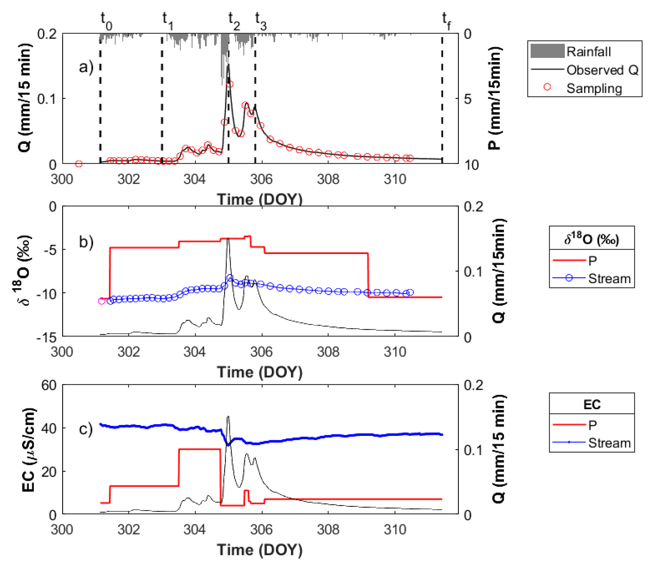
The monitored rainfall-runoff event lasted for 10 days and 6.5 h (t0 − tf in Figure 3a). During this period, total precipitation (in the form of rain; P) and total runoff (Q) reached 155.1 mm and 20.6 mm, respectively. These values corresponded to a runoff coefficient (Q/P) of 0.13. During the first 44.5 h (t0 − t1), total P was 19.9 mm with a mean intensity of 0.45 mm h−1. This period was characterized by little response in the hydrograph. Subsequently (t1 − t2), Q started to increase in response to P inputs of higher intensity (0.95 mm h−1). At t2 (92.5 h since t0) Q reached its maximum after a total P amount of 107.4 mm. Later (t2 − t3), the recession of the hydrograph started as P intensity decreased to 0.30 mm h−1. Then, at t3, the last Q peak occurred 112 h after the beginning of the event. By this time, total P was 140.7 mm. Between t3 and the end of the event (tf), P almost completely ceased, and the hydrograph recession proceeded. During this last period (t3 − tf), total P was 14.4 mm with a mean intensity of 0.06 mm h−1.
The temporal dynamics of the δ18O and EC signals of P and Q are shown in Figure 3b,c respectively. The δ18O of P (δ18OP) at t0 (baseline signal) was the lowest during the event (−10.66 ‰) and started increasing as P inputs increased (Figure 3b). The δ18OP signal peaked at −3.5‰ in the water sample collected a few hours before the Q peak at t3. After this time, during the recession of the hydrograph, the δ18OP decreased to the baseline value in the sample collected at the end of the event (tf). Similarly, the EC signal in P (ECP) started at a low baseline value of 5.2 μS cm−1, and increased as P inputs increased (Figure 3c). The ECP peaked at a value of 30 μS cm−1 in the sample collected a few hours before the highest peak of the hydrograph at t2. After this period, ECP decreased near the baseline value, and then peaked again (as δ18OP did) in the sample collected before the last Q peak (around t3) with a value of 11 μS cm−1. Then, ECP decreased to the baseline value during the recession of the Q as P inputs decreased until the end of the event (tf). The temporal variability in the Q δ18O (δ18OQ) was smaller (−10.92‰ to −8.3‰; Figure 3b) than the variability observed in δ18OP. The δ18OQ showed a pattern related to the hydrograph, i.e., δ18OQ increased as Q increased, and vice versa, in response to the dynamics of P. Similarly, the temporal change of EC in Q (ECQ) was lower (31.8–41.6 μS cm−1; Figure 3c) than ECP. The ECQ variability was the mirror image of the δ18OQ signal, i.e., when the δ18OQ signal (and Q) increased, the ECQ signal decreased, and vice versa (the r2 between EC and δ18O. is 0.69). The Q values of the pre-event water fraction were −10.92‰ for δ18O and 41.0 μS for EC.
3.2. Model Performance
A summary of the parameter values that yielded the highest NSEs and the statistics of the calibration model performance for the four structures using each tracer are presented in Table 2 and Table 3 respectively. In general, all model structures using both tracers yielded strong fits (NSE > 0.79) to the observed Q and tracer data (Table 3). The highest NSEs were obtained using model structures 2 and 4 (NSE = 0.87) for δ18O and model structure 4 (NSE = 0.90) for EC. Our evaluation of the models structures’ parsimoniousness showed that the variation of the AIC values for Q (10,747–22,581) was higher than the variation of the AIC values for the tracers (213–1025) among the different model structures (Table 3). Even though model structure 4 had the largest number of fitting parameters, the sum of the AIC values for Q and the tracers (ΣAIC) showed that this model structure yielded the lowest values for both δ18O (ΣAIC = 12,238) and EC (ΣAIC = 10,992).
3.3. Modelled Streamflow Partitioning
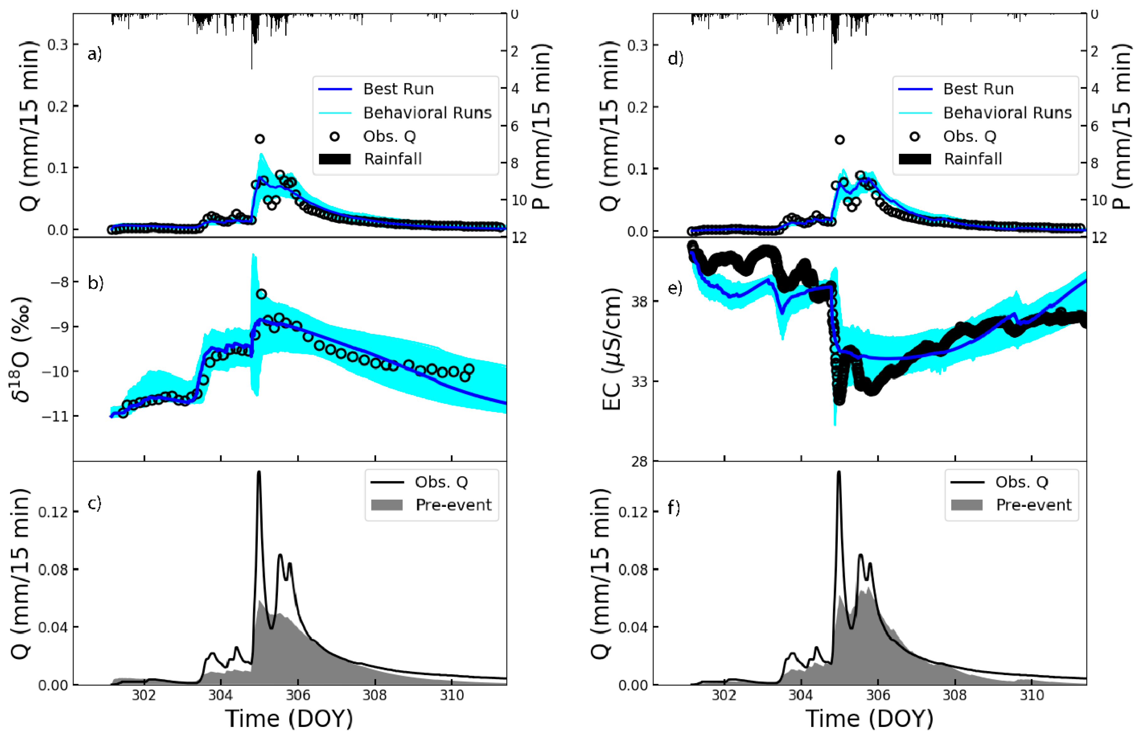
The fitted hydrographs using TRaSPAN model structure 1 (Figure 2a) for δ18O and EC (Figure 4a,d) poorly resembled the temporal dynamics of Q during the monitored event. In general, the model was not able to reproduce the Q peak responses to P inputs, or the recession limbs of the hydrographs. This was particularly noticeable during the highest Q peak and rapid recession of the hydrograph on DOY 305 and by the overestimation (DOY 306–308) and underestimation (DOY 308–311) of Q during the recession limb of the hydrograph. Similarly, this model structure poorly reproduced the δ18OQ and ECQ temporal variability during the event. The structure could not resemble the δ18OQ tracer signal dynamics at the beginning of the event (DOY 301–303) and the enriched isotopic composition during the highest Q peak response on DOY 306 (Figure 4b). During the remaining of the event, the tracer signal was better captured within the uncertainty bands of the simulations. Regarding the ECQ temporal dynamics, the model simulations were even weaker (Figure 4e). The model poorly reproduced this tracer’s signal at the beginning of the event (DOY 301–304), during the highest Q peak response (DOY 305), and during the last part of the event’s recession limb (DOY 311). The pre-event water fractions estimated using this model structure were 71.7% for δ18O and 79.6% for EC (Table 3) and the temporal dynamics of the event and pre-event water contributions to total Q are shown in Figure 4c,f, respectively. These fractions depicted similar overall model results using both tracers. Our simulations also indicated an over prediction of the pre-event water fraction (i.e., Qe > 100%) at the beginning of the event with δ18O (DOY 301–302; Figure 4c) and at the first part of the recession limb (DOY 306–308; Figure 4d) with EC. Similar results were found for model structure 3 (time-variant fraction of Peff routed as event water and single reservoirs for event and pre-event; Figure 2c). For this structure, the implementation of the time-variant routine for the fraction of Peff routed as event water did not improve the simulations of the hydrograph and the temporal variation of the tracers (Figure S2). The pre-event water fractions estimated using this model structure were 76.3% for δ18O and 81.7% for EC (Table 3) and the temporal dynamics of the event and pre-event water contributions to total Q were similar using both tracers (Figure S2c,f).
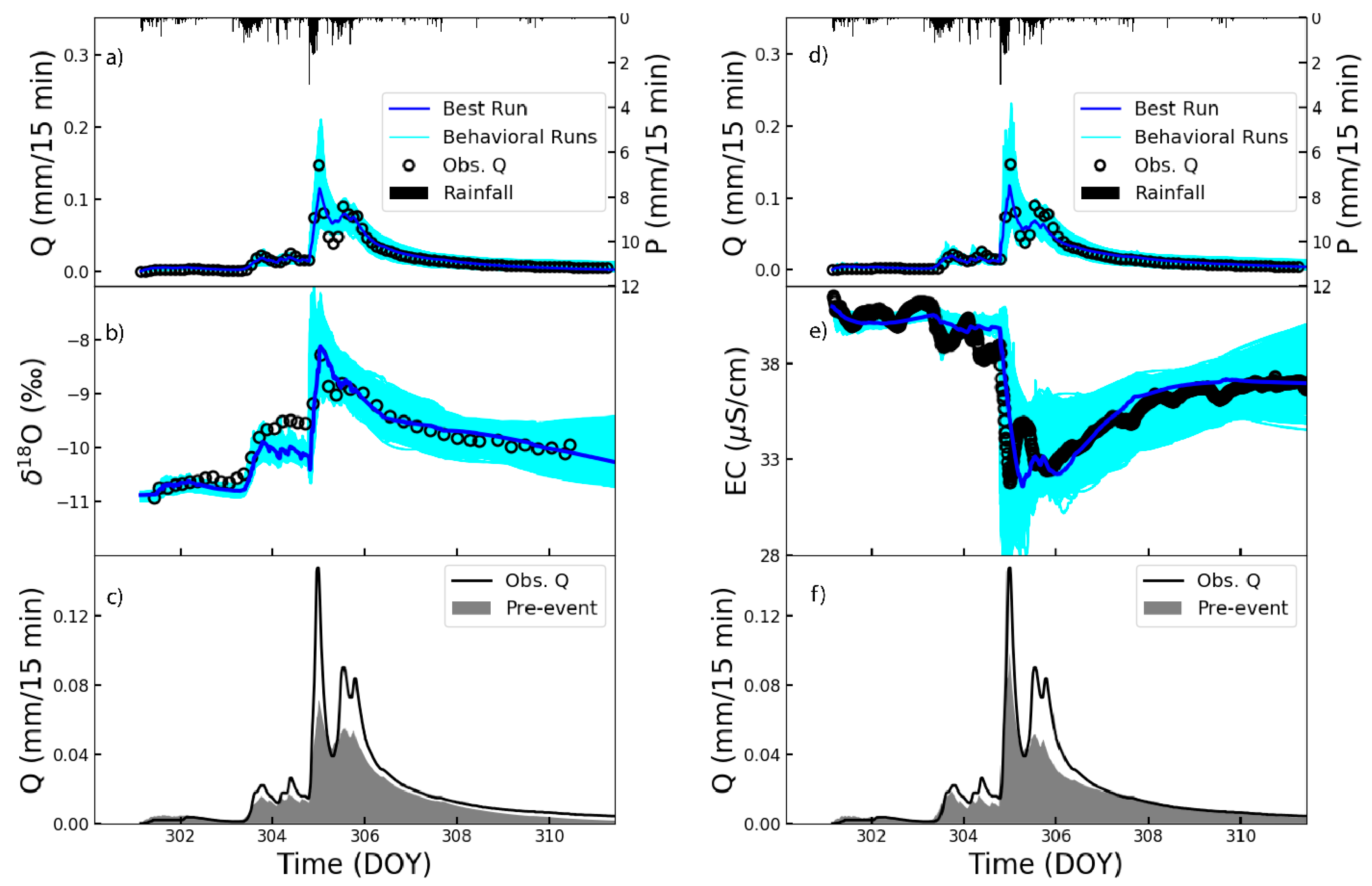
The simulation results using TRaSPAN model structure 4 (i.e., the time variant fraction of Peff routed as event water and two connected reservoirs for event and pre-event water; Figure 2d) showed that this structure better captured the temporal dynamics of Q using both tracers. All peaks (e.g., the highest peak produced on DOY 305) and the recession (DOY 306–311) of the hydrograph were well simulated by this model structure using δ18O (Figure 5a) and EC (Figure 5d). Similarly, the temporal dynamics of the tracers’ signal were well simulated by this model structure. Even though this model structure underestimated the δ18OQ enrichment (Figure 5b) and overestimated the decrease in ECQ (Figure 5e) on DOY 304; the most enriched δ18OQ and the lowest ECQ peak values (DOY 305), as well as the rest of the tracer dynamics, fitted the observed data well. The estimated proportions of pre-event water were 74.9% using δ18O and 81% using EC (Table 3). The temporal variability of the pre-event water contributions were similar using δ18O (Figure 5c) and EC (Figure 5f) and showed a dominance of pre-event water contributions, even during the peak Q generation.
Even though structure 2 (i.e., the constant fraction of Peff routed as event water and two connected reservoirs for event and pre-event; Figure 2b), simulated the hydrograph better than structures 1 and 3 using both tracers (e.g., it captured the Q peaks better), it still had issues simulating the peak hydrograph response compared to structure 4, particularly when calibrated using δ18O (Figure S1a,b). Structure 2 also had issues replicating the δ18OQ (Figure S1c) and ECQ (Figure S1d), particularly when calibrated using EC during the rising limb of the hydrograph. The pre-event water fractions estimated using this model structure were 76.2% for δ18O and 79.5% for EC (Table 3). However, in contrast to all of the other model structures, the temporal dynamics of the event and pre-event water contributions to total Q were different using both tracers. This structure tended to estimate lower pre-event water contributions during the rising limb of the hydrograph and higher pre-event water contributions during the recession when calibrated using δ18O (Figure S1c). An opposite trend was observed when calibrated for EC (Figure S1f).
3.4. Model Parameter Identification for the Best Model Structure
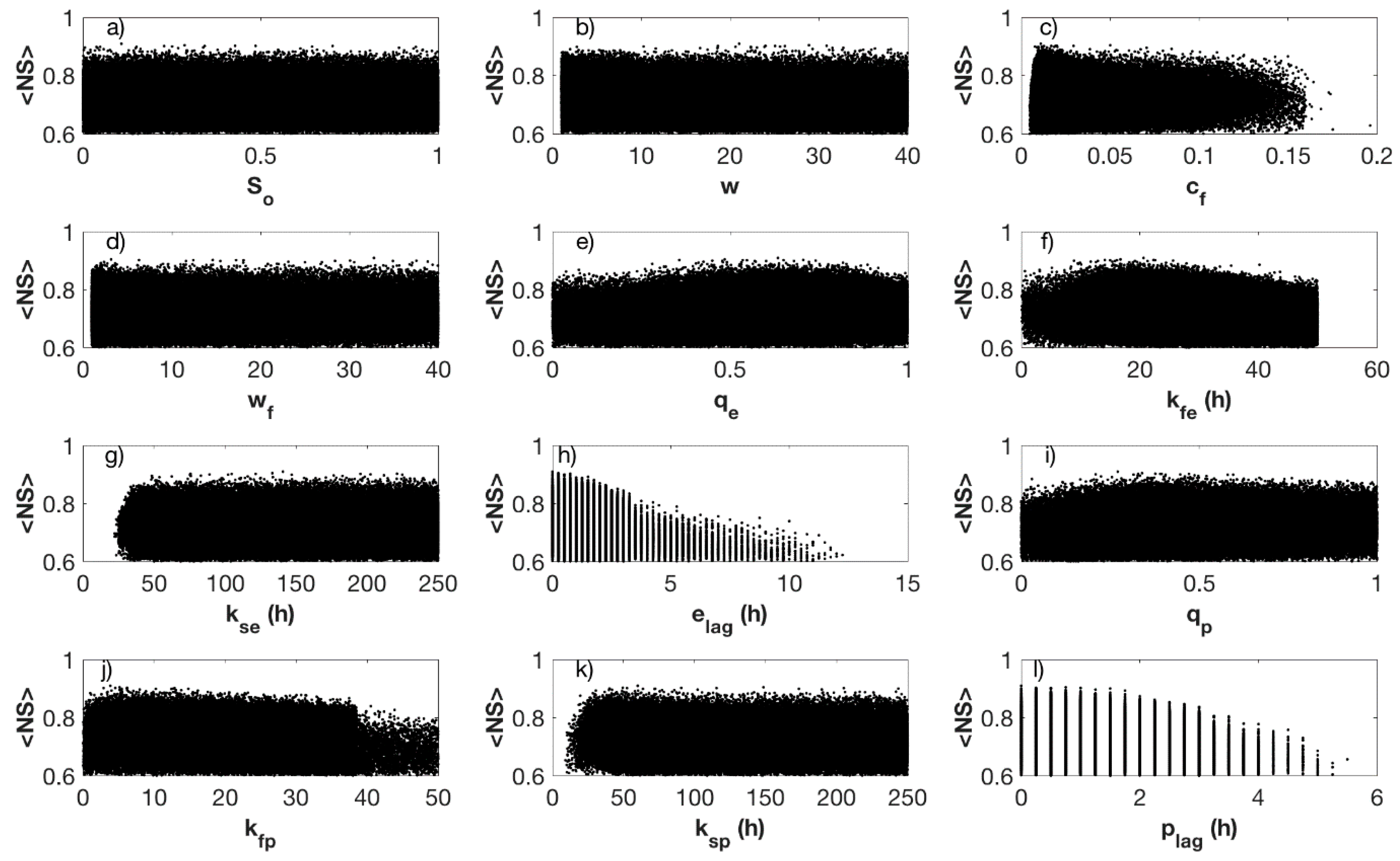
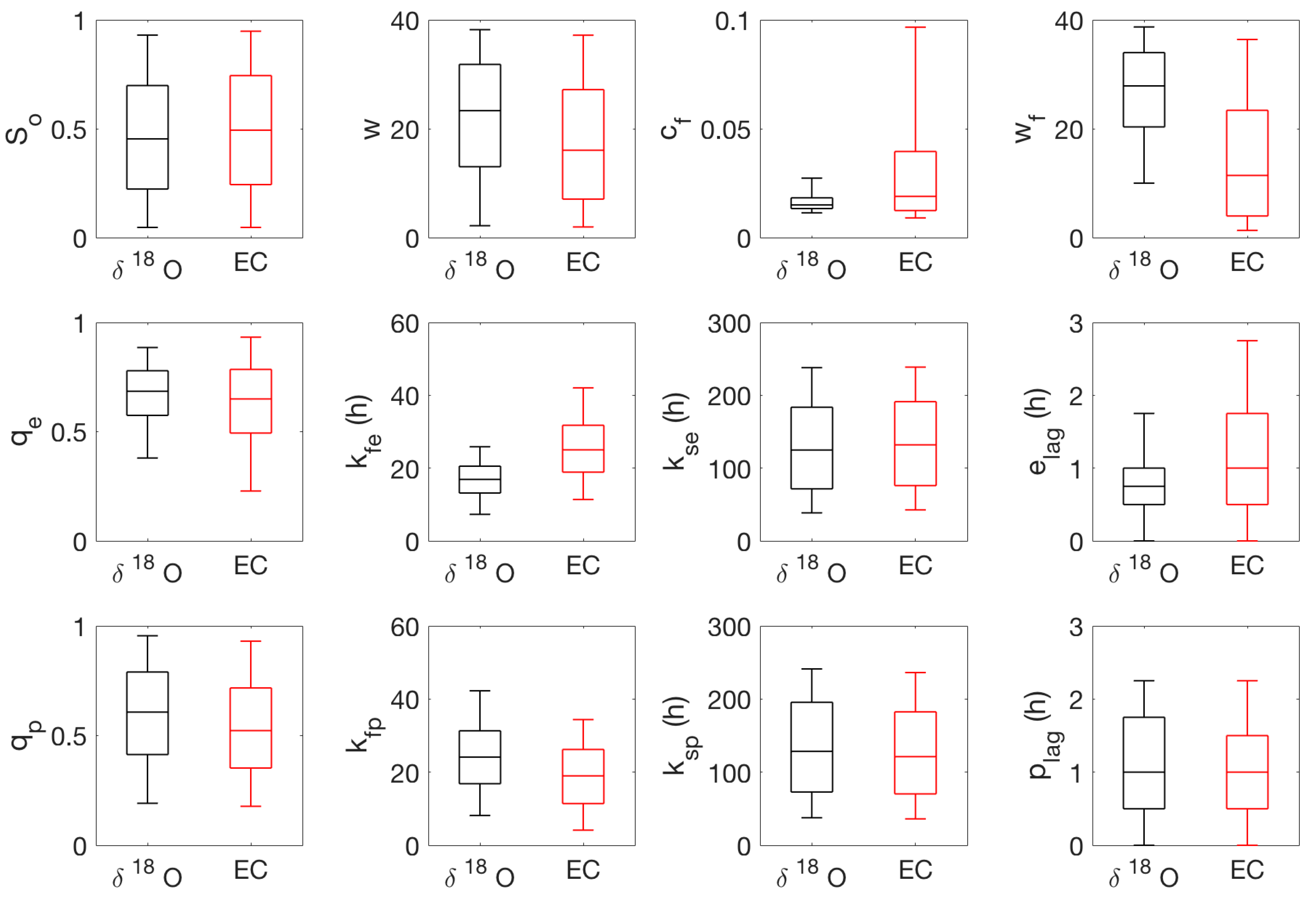
According to the dotty plots (i.e., values of the NSE as a function of the calibrated parameters for a given model run), seven of the 12 parameters of model structure 4 using EC for calibration reached a single peak in the parameter space yielding the highest NSE (Figure 6). These parameters were: the normalization constant (cf = 0.01; Figure 6c; Table 2) of module 2 and the fraction of water routed into the fast-responding reservoir of event water (qe = 0.63; Figure 6e), the mean transit time (MTT) of the fast fraction of event water (kfe = 20.62 h; Figure 6f), the time delay for the event fraction response (elag = 0 h; Figure 6h), the fraction of water routed into the fast-responding reservoir of pre-event water (qp = 0.27; Figure 6i), and the MTT of the fast fraction of pre-event water (kfp = 3.84 h; Figure 6j), and the time delay for the pre-event fraction response (plag = 0 h; Figure 6l) of module 3. Both parameters of module 1 (So; Figure 6a and w; Figure 6b), the memory timescale parameter (wf) of module 2 (Figure 6d), and the slow fractions of event (kse; Figure 6g) and pre-event (ksp; Figure 6k) water of module 3 showed equifinality [79]. That is, these parameters did not reach a single peak associated to the highest NSE in their parameter space distributions. The distributions of the model parameters for model structure 4 calibrated using δ18O was similar (Figure S9) and the ranges of calibrated parameters using both tracers were in strong agreement (Figure 7).
Similar results were found for model structure 2 using EC for calibration. For this structure, the module 3 parameters qe, kfe, elag, qp, kfp, and plag, as well as the constant fraction of effective rainfall routed as event water parameter f (module 2) reached a single peak in the parameter space yielding the highest NSE (i.e., seven out of 11 parameters; Figure S6). However, even tough for the same model structure calibrated using δ18O, the parameters qp and kfp did not reach a single peak in the parameter space (i.e., only five out of 11 parameters did; Figure S5), the ranges of calibrated parameters using both tracers were in agreement (Figure S11).
For model structure 1 calibrated using EC, none of the parameters of module 1 reached a single peak in the parameter space, whereas the parameters f (module 2), and ke, elag, kp, and plag (module 3) did (i.e., five out of seven parameters; Figure S4). The calibration of structure 1 using δ18O, showed that the parameter w (module 1) reached a single peak in the parameter space in addition to those that did for the model calibrated for EC (i.e., six out of seven parameters; Figure S3). Similarly, the ranges of the calibrated parameters for both tracers were not in agreement (Figure S10). For model structure 3 calibrated using EC, only the cf parameter (module 2), and the ke, kp, and elag parameters (module 3) reached a single peak in the parameter space (i.e., four out of eight parameters; Figure S8). The same parameters reach a single peak in the parameter space when structure 3 was calibrated using δ18O (Figure S7) and the ranges of calibrated parameters using both tracers were in agreement (Figure S12).
3.5. Comparison of Model Results for Both Tracers
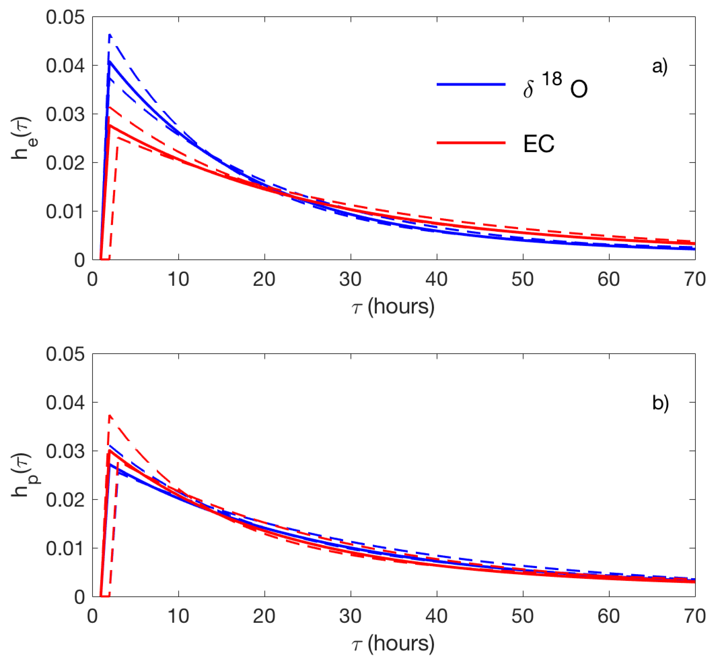
Even though the TTDs of the event fractions using both tracers were similar for transit times (τ) longer than 20 h (Figure 8), there was some discrepancy in the τ distributions shorter than 20 h. For shorter τ, the calibration with δ18O yielded a TTD with a predominance of shorter τ in comparison to the calibration of the model calibrated with EC (Figure 8a). The shape of the TTDs of the pre-event water fractions (Figure 8b) were opposite to those of the event water fraction. That is, for shorter MTTs (<10 h), there was a predominance of shorter MTTs for the calibration with EC compared to the calibration with δ18O.
4. Discussion
4.1. Selection of the Best Model Structure Using Water Isotopes and Electrical Conductivity for Model Calibration
The various TraSPAN model structures can be used to test different hypothesis about the processes that control streamflow generation [69,70] or as a rejectionist framework to improve knowledge about the hydrological behavior of a given catchment [26]. Thus, the modeler can hypothesize and test different hydrological behaviors and assumptions in a catchment by building and testing conceptual models that represent different catchment functions [80,81].
In our study, the four tested model structures (i.e., competing hypotheses [82,83]) provided strong fits in terms of the NSE objective function using both tracers for calibration (NSEs > 0.79; Table 3). However, further evaluation of the models’ parsimoniousness, depicted important differences among the evaluated structures (Table 3). The simplest TraSPAN structures, including a single reservoir for the event and pre-event water transit times assuming either constant (structure 1 with 7 parameters; Figure 2a) or a time variant (structure 3 with 8 parameters; Figure 2c) fraction of Peff routed as event water, provided less parsimonious results than the more complex structures 2 and 4. Between structures 2 and 4, which represented the catchment response with two connected linear reservoirs for each the event and pre-event water fractions and a constant (structure 2 with 11 parameters; Figure 2b) or time variant (structure 4 with 12 parameters; Figure 2d) fraction of Peff routed as event water; structure 4 was the most parsimonious to represent the internal catchment response using both tracers (Table 3).
Regarding the results of the simulations of the observed Q and tracer data, the simplest structures 1 and 3 poorly resembled the hydrograph. These structures did not reproduce the peak responses and the recessions that followed them (DOY 306–311; Figure 4a,d, Figure S2a,d). Regarding the simulation of the tracer dynamics, these structures captured relatively well the δ18OQ decrease and ECQ increase during the hydrograph falling limb but poorly resembled the tracer dynamics at the beginning of the event (Figure 4b,e, Figure S2b,e). These results indicate that the hydrological behavior of Mack Creek is not well represented when a single reservoir is used to route the event and pre-event water fractions regardless of the treatment of the Peff as constant or time variant. On the other hand, structures 2 and 4 provided better representations of the hydrograph and the tracers’ dynamics. Both of these structures calibrated with both tracers were able to better resemble the highest Q peak (DOY 305) and the following rapid recession (Figure 5a,d, Figure S1a,d). These results suggest that the Mack Creek hydrological system is better represented by two connected linear reservoirs for each the event and pre-event water fractions. Regarding the tracer dynamics, structure 4 provided the best fits of the tracer data in comparison with structure 2 for both tracers (Figure 5b,e, Figure S1b,e). These results indicate that the system is not only better represented by two connected reservoirs, but that the internal mixing of the tracer is better represented when the Peff routed as event water is treated as time-variant (structure 4) than when it is treated as constant (structure 2). Even though not directly investigated at Mack Creek evidence of non-stationary flow conditions and tracer dynamics have been shown for WS10, a 0.1 km2 catchment located near the outlet of the H.J. Andrews Forest (Figure 1) [63,84,85].
4.2. Comparison of Flow Partitioning Modelling Results Calibrated for Water Isotopes and Electrical Conductivity
The ranges of the calibrated parameters for TraSPAN structure 4 were remarkably similar using both WSI and EC for calibration (Figure 6 and Figure 7, and Figure S9, and Table 2). In addition, the temporal variation (Figure 5c,f) and the estimated proportions of pre-event water yielded by the model calibrated for each tracer were in agreement (74.9% for δ18O and 81.0% for EC, Table 3). Even though previous hydrograph separation investigations using simple tracer mixing models have found contradictory results regarding the reliability of the event and pre-event water contributions when EC is used as a tracer due to its non-conservative nature [16,18,48,50,51,53,86,87,88], our findings suggest that this issue could be related to the lack of simultaneous representation of the water flow transport in addition to the tracer mixing within a given hydrological system. We were able to account for both using our TraSPAN numerical modeling approach.
Similar findings were reported by Mosquera et al. [76] in a study conducted to evaluate the baseflow transit times in a nested system of tropical alpine (páramo) catchments in South America. These authors found that the spatial variability of transit time estimates for their nested system of catchments—based on the calibration of a lumped conceptual model using δ18O—was highly correlated with the catchments’ mean yearly baseflow EC (r2 = 0.89) and suggested that average EC values could be used as an inexpensive proxy to estimate baseflow transit times. Even though these results cannot be generalized until additional investigations are carried out in different environments, the results from Mosquera et al. [76] and our study highlight the potential advantages of high-resolution monitoring of EC for hydrological modelling applications, particularly when flow dynamics are accounted for.
4.3. On the Use of High-Temporal Resolution EC in Hydrograph Separation Modelling
It is worth noting that the structure 4 simulation results yielded better model performance, both in terms of goodness of fit and parsimoniousness, when calibrated with the finer temporal resolution of EC data than when calibrated for δ18O (Table 3). The simulation results also showed that a higher accuracy to represent the hydrograph and tracer dynamics was obtained when structure 4 was calibrated using the higher-resolution EC data (sub-hourly), than when calibrated for WSI data collected every 4 h. For instance, the hydrograph highest peak and following recession on DOY 305 (Figure 5a,c) and the rapid δ18O increase/EC decrease on DOY 304–305 (Figure 5b,d) were better represented by the model calibrated using EC data. These results indicate that even though the model calibrated for both tracers depicted similar hydrological behavior (see Section 4.4 for details), the calibration for the higher-resolution EC data allowed better capturing of the fast occurrence of flow transport and solute mixing processes. These simulations resulted in the release of higher amounts of pre-event water for the model calibrated for EC (81%), particularly during the highest hydrograph peak on DOY 305 (Figure 5f), with respect to the calibration for δ18O (75%; Figure 5c).
Other investigations have also reported higher accuracy to represent the temporal variability of the tracer’s signal, and further interpretation of water routing in hydrological systems when using high-temporal resolution tracer data [89,90]. Our results do not only support the findings from these authors, but also demonstrate the potential of the inexpensive collection of EC data at high-temporal resolution to improve understanding of fast occurring (seconds to minutes) hydrological processes.
4.4. Process-Based Understanding of Hydrological Behavior
We evaluated the similarity in hydrological behavior of the transport and mixing of water within the Mack Creek catchment based on the shapes of TTDs provided by the best model structure calibrated for each tracer. Despite the overall similarities of the TTDs’ shapes for both tracers (Figure 8) with dominance of long transit times (τ > 10 h), our results showed small differences for shorter transit times (τ < 20 h for the event water fractions, Figure 8a; τ < 10 h for the pre-event water fractions, Figure 8b). This discrepancy could be related to different temporal resolution of the data used for calibration, as reported in other studies [89]. In other words, the use of finer temporal resolution EC data (every 0.25 h) in comparison to the WSI data (every 4 h).
From a process-based perspective, the TTDs obtained from the model calibration using both tracers indicate that the catchment acts as a connected system of two water reservoirs each with a fast and a slow transit function contributing large amounts of pre-event water (75–81%) to discharge (Table 3). These two reservoirs likely represent: (1) fast event and pre-event water moving through the shallow permeable soils and (2) slow event and pre-event water moving through the fractured parent material (hereafter referred to as the groundwater reservoir, GW). That is, this catchment has poorly developed gravelly loam soils with high infiltration rates (>500 cm h−1) that are overlaying highly weathered and fractured bedrock [57]. Baseflow MTT at Mack Creek was estimated around 2 ± 0.49 years, i.e., one of the longest within the H.J. Andrews catchments [57]. This MTT estimation indicates that water is likely stored in the GW reservoir, as has been observed in other headwater catchments with relatively permeable geology (e.g., [73,91,92]). Stored water that can be released rapidly to streams during rainfall events given the connectivity between hillslopes and riparian areas. Such connectivity has been observed near our study area at WS10 (Figure 1) [63]. Additionally, even though high amounts of pre-event water were released as streamflow during the monitored event, the total runoff (20.6 mm) accounted for only 13% of the total precipitation input (155.1 mm). Again, given the permeable soils and fractured bedrock of the catchment, and the dry antecedent moisture conditions during the monitoring period (28 October–7 November)—which corresponded to the beginning of the fall season after the summer period in the particularly dry water year 2015—only a small fraction of total precipitation was converted into Peff. These results from the hydrometric analysis indicate that the rest of water inputs must have filled the initially low water storage of the GW reservoir after the dry summer. In this context, the strong goodness of fit of our model to simulate the high temporal variability of the streamflow and tracer data dynamics (Figure 5a–d) indicates that through the simultaneous calibration of water and solute fluxes, our model was not only capable to successfully account for the water flux and tracer mixing dynamics, but also for the recharge of water in the groundwater system.
5. Concluding Remarks and Future Directions
Our evaluation of a tracer-based hydrological model (TraSPAN) demonstrated that the assessment of different modeling structures—each representing a different rainfall-runoff response—allowed for a better identification of the hydrological system functioning. For our analyzed rainfall event at the H.J. Andrews experimental forest, we found that the same model structure was best at representing hydrographic and tracer dynamics using either electrical conductivity/specific conductance (EC) or water-stable isotopes (WSIs) collected at high temporal resolution for calibration. The model results using both tracers not only showed a remarkable agreement to fit the observed data and the calibrated parameter distributions, but also in terms of the process-based understanding of the hydrological system. Moreover, the use of sub-hourly (0.25 h) collected EC data also allowed to better simulate the catchment hydrological response in comparison to the 4 h δ18O data. These findings highlight the potential of using low-cost EC data collected at high temporal resolution in combination with a flexible hydrological modelling framework to better understand catchment hydrological behavior.
Despite the advantages of our applied methodology, we acknowledge that before the widespread application of our approach, future research should focus on understanding site-dependent geochemical conditions under which the applicability of EC as a conservative tracer is suitable. Future research should also focus on implementing monitoring strategies that allow for the combined collection of water isotopes and geochemical data at the highest possible temporal resolution during a variety of climatic conditions (i.e., wet, transition, and dry periods). We encourage such efforts, as these data would provide information about the spatial and temporal variability in weathering rates to better establish the conditions under which the use of high-resolution EC observations would yield robust datasets to investigate important, but yet unresolved, questions in catchment hydrology that require the identification of fast-occurring hydrological processes, while reducing monitoring costs and the degree of uncertainty in simulated flow components.
Supplementary Materials
The following are available online at https://www.mdpi.com/2073-4441/10/7/904/s1.
Author Contributions
Conceptualization, C.S. and G.M.M.; Methodology, C.S. Formal Analysis, G.M.M., C.S., and P.C., Resources, C.S. and P.C; Data Curation, C.S. Writing-Original Draft Preparation, G.M.M. and C.S. Writing-Review & Editing, G.M.M., C.S., and P.C.; Project Administration, C.S.; Funding Acquisition, C.S. and P.C.
Funding
This research was funded in part by National Science Foundation under grant No. DEB-1440409, by the USDA National Institute of Food and Agriculture; McIntire Stennis project OREZ-FERM-876., and by the General Research Fund of Oregon State University. G.M.M. and P.C. were funded by the Secretaría Nacional de Educación Superior, Ciencia, Tecnología e Innovación del Ecuador (SENESCYT) and the Central Research Office (DIUC) (project PIC-13-ETAPA-001); and by the Doctoral Program in Water Resources of the University of Cuenca.
Acknowledgments
We would like to thank Lydia Nickolas for collecting the storm water samples and Markus Weiler for feedback on the model description. Data and facilities were provided by the HJ Andrews Experimental Forest and Long Term Ecological Research program, administered cooperatively by the USDA Forest Service Pacific Northwest Research Station, Oregon State University, and the Willamette National Forest. This material is based upon work supported by the National Science Foundation under Grant No. DEB-1440409. The isotopic data collected will be submitted to the IAEA Global Network of Isotopes in Rivers.
Conflicts of Interest
The authors declare no conflict of interest.
References
- Kendall, C.; McDonnell, J.J. Isotope Tracers in Cacthment Hydrology; Elsevier Science B.V.: Amsterdam, The Netherlands, 1998. [Google Scholar]
- Burns, D.A.; Kendall, C. Analysis δ15N and δ18O to Differentiate NO3− Sources in Runoff at Two Watersheds in the Catskill Mountains of New York. Water Resour. Res. 2002, 38, 9-1–9-11. [Google Scholar] [CrossRef]
- Hrachowitz, M.; Fovet, O.; Ruiz, L.; Savenije, H.H.G. Transit time distributions, legacy contamination and variability in biogeochemical 1/fα scaling: How are hydrological response dynamics linked to water quality at the catchment scale? Hydrol. Process. 2015, 29, 5241–5256. [Google Scholar] [CrossRef]
- Burt, T.P.; Pinay, G. Linking hydrology and biogeochemistry in complex landscapes. Prog. Phys. Geogr. 2005, 29, 297–316. [Google Scholar] [CrossRef]
- Buttle, J.M. Isotope hydrograph separations and rapid delivery of pre-event water from drainage basins. Prog. Phys. Geogr. 1994, 18, 16–41. [Google Scholar] [CrossRef]
- Klaus, J.; Mcdonnell, J.J. Hydrograph separation using stable isotopes: Review and evaluation. J. Hydrol. 2013, 505, 47–64. [Google Scholar] [CrossRef]
- Heidbüchel, I.; Troch, P.A.; Lyon, S.W.; Weiler, M. The master transit time distribution of variable flow systems. Water Resour. Res. 2012, 48, W06520. [Google Scholar] [CrossRef]
- Hrachowitz, M.; Savenije, H.H.G.; Blöschl, G.; McDonnell, J.J.; Sivapalan, M.; Pomeroy, J.W.; Arheimer, B.; Blume, T.; Clark, M.P.; Ehret, U.; et al. A decade of predictions in ungauged basins (pub)—A review. Hydrol. Sci. J. 2013, 58, 1198–1255. [Google Scholar] [CrossRef]
- Birkel, C.; Soulsby, C.; Tetzlaff, D.; Dunn, S.; Spezia, L. High-frequency storm event isotope sampling reveals time-variant transit time distributions and influence of diurnal cycles. Hydrol. Process. 2012, 26, 308–316. [Google Scholar] [CrossRef]
- Kirchner, J.W. Aggregation in environmental systems—Part 1: Seasonal tracer cycles quantify young water fractions, but not mean transit times, in spatially heterogeneous catchments. Hydrol. Earth Syst. Sci. 2016, 20, 279–297. [Google Scholar] [CrossRef]
- Rinaldo, A.; Beven, K.J.; Bertuzzo, E.; Nicotina, L.; Davies, J.; Fiori, A.; Russo, D.; Botter, G. Catchment travel time distributions and water flow in soils. Water Resour. Res. 2011, 47. [Google Scholar] [CrossRef] [Green Version]
- Van der Velde, Y.; Heidbüchel, I.; Lyon, S.W.; Nyberg, L.; Rodhe, A.; Bishop, K.; Troch, P.A. Consequences of mixing assumptions for time-variable travel time distributions. Hydrol. Process. 2015, 29, 3460–3474. [Google Scholar] [CrossRef]
- Rode, M.; Wade, A.J.; Cohen, M.J.; Hensley, R.T.; Bowes, M.J.; Kirchner, J.W.; Arhonditsis, G.B.; Jordan, P.; Kronvang, B.; Halliday, S.J.; et al. Sensors in the stream: The high-frequency wave of the present. Environ. Sci. Technol. 2016, 50, 10297–10307. [Google Scholar] [CrossRef] [PubMed]
- Hooper, R.P.; Shoemaker, C.A. A Comparison of chemical and isotopic hydrograph separation. Water Resour. Res. 1986, 22, 1444–1454. [Google Scholar] [CrossRef]
- Hooper, R.P.; Christophersen, N.; Peters, N.E. Modelling streamwater chemistry as a mixture of soilwater end-members—An application to the Panola Mountain catchment, Georgia, U.S.A. J. Hydrol. 1990, 116, 321–343. [Google Scholar] [CrossRef]
- Laudon, H.; Slaymaker, O. Hydrograph separation using stable isotopes, silica and electrical conductivity: An alpine example. J. Hydrol. 1997, 201, 82–101. [Google Scholar] [CrossRef]
- Uhlenbrook, S.; Hoeg, S. Quantifying uncertainties in tracer-based hydrograph separations: A case study for two-, three- and five-component hydrograph separations in a mountainous catchment. Hydrol. Process. 2003, 17, 431–453. [Google Scholar] [CrossRef]
- Kronholm, S.C.; Capel, P.D. Estimation of time-variable fast flow path chemical concentrations for application in tracer-based hydrograph separation analyses. Water Resour. Res. 2016, 52, 6881–6896. [Google Scholar] [CrossRef]
- Pinder, G.F.; Jones, J.F. Determination of the ground-water component of peak discharge from the chemistry of total runoff. Water Resour. Res. 1969, 5, 438–445. [Google Scholar] [CrossRef]
- Sklash, M.G.; Farvolden, R.N. Role of groundwater in storm runoff. J. Hydrol. 1979, 43, 45–65. [Google Scholar] [CrossRef]
- Laudon, H.; Seibert, J.; Köhler, S.; Bishop, K. Hydrological flow paths during snowmelt: Congruence between hydrometric measurements and oxygen 18 in meltwater, soil water, and runoff. Water Resour. Res. 2004, 40. [Google Scholar] [CrossRef]
- Rice, K.C.; Hornberger, G.M. Comparison of hydrochemical tracers to estimate source contributions to peak flow in a small, forested, headwater catchment. Water Resour. Res. 1998, 34, 1755–1766. [Google Scholar] [CrossRef] [Green Version]
- McDonnell, J.J.; Kendall, C. Isotope tracers in hydrology. Eos Trans. Am. Geophys. Union 1992, 73, 260–261. [Google Scholar] [CrossRef]
- Roa-Garcia, M.; Weiler, M. Integrated response and transit time distributions of watersheds by combining hydrograph separation and long-term transit time modeling. Hydrol. Earth Syst. Sci. 2010, 14, 1537–1549. [Google Scholar] [CrossRef] [Green Version]
- Segura, C.; James, A.L.; Lazzati, D.; Roulet, N.T. Scaling relationships for event water contributions and transit times in small-forested catchments in Eastern Quebec. Water Resour. Res. 2012, 48, W07502. [Google Scholar] [CrossRef]
- Vaché, K.B.; McDonnell, J.J. A process-based rejectionist framework for evaluating catchment runoff model structure. Water Resour. Res. 2006, 42. [Google Scholar] [CrossRef] [Green Version]
- Weiler, M.; McGlynn, B.L.; McGuire, K.J.; McDonnell, J.J. How does rainfall become runoff? A combined tracer and runoff transfer function approach. Water Resour. Res. 2003, 39. [Google Scholar] [CrossRef] [Green Version]
- Barnes, C.J.; Bonell, M. Application of unit hydrograph techniques to solute transport in catchments. Hydrol. Process. 1996, 10, 793–802. [Google Scholar] [CrossRef]
- Kirchner, J.W.; Feng, X.; Neal, C. Fractal stream chemistry and its implications for contaminant transport in catchments. Nature 2000, 403, 524–527. [Google Scholar] [CrossRef] [PubMed]
- McGuire, K.J.; McDonnell, J.J. A review and evaluation of catchment transit time modeling. J. Hydrol. 2006, 330, 543–563. [Google Scholar] [CrossRef]
- Hrachowitz, M.; Benettin, P.; van Breukelen, B.M.; Fovet, O.; Howden, N.J.K.; Ruiz, L.; van der Velde, Y.; Wade, A.J. Transit times-the link between hydrology and water quality at the catchment scale. Wiley Interdiscip. Rev. Water 2016, 3, 629–657. [Google Scholar] [CrossRef] [Green Version]
- Maloszewski, P.; Zuber, A. Determining the turnover time of groundwater systems with the aid of environmental tracers 1. Models and their applicability. J. Hydrol. 1982, 57, 207–231. [Google Scholar] [CrossRef]
- Brooks, J.R.; Barnard, H.R.; Coulombe, R.; McDonnell, J.J. Ecohydrologic separation of water between trees and streams in a Mediterranean climate. Nat. Geosci. 2010, 3, 100–104. [Google Scholar] [CrossRef]
- Coplen, T.B.; Neiman, P.J.; White, A.B.; Landwehr, J.M.; Ralph, F.M.; Dettinger, M.D. Extreme changes in stable hydrogen isotopes and precipitation characteristics in a landfalling Pacific storm. Geophys. Res. Lett. 2008, 35, L21808. [Google Scholar] [CrossRef]
- Coplen, T.B.; Neiman, P.J.; White, A.B.; Ralph, F.M. Categorisation of northern California rainfall for periods with and without a radar brightband using stable isotopes and a novel automated precipitation collector. Tellus B 2015, 67, 28574. [Google Scholar] [CrossRef]
- Munksgaard, N.C.; Wurster, C.M.; Bass, A.; Bird, M.I. Extreme short-term stable isotope variability revealed by continuous rainwater analysis. Hydrol. Process. 2012, 26, 3630–3634. [Google Scholar] [CrossRef]
- McDonnell, J.J.; Bonell, M.; Stewart, M.K.; Pearce, A.J. Deuterium variations in storm rainfall: Implications for stream hydrograph separation. Water Resour. Res. 1990, 26, 455–458. [Google Scholar] [CrossRef]
- Berman, E.S.F.; Gupta, M.; Gabrielli, C.; Garland, T.; McDonnell, J.J. High-frequency field-deployable isotope analyzer for hydrological applications. Water Resour. Res. 2009, 45, W10201. [Google Scholar] [CrossRef]
- Munksgaard, N.C.; Wurster, C.M.; Bass, A.; Zagorskis, I.; Bird, M.I. First continuous shipboard δ18O and δD measurements in sea water by diffusion sampling—Cavity ring-down spectrometry. Environ. Chem. Lett. 2012, 10, 301–307. [Google Scholar] [CrossRef]
- Munksgaard, N.C.; Wurster, C.M.; Bird, M.I. Continuous analysis of δ18O and δD values of water by diffusion sampling cavity ring-down spectrometry: A novel sampling device for unattended field monitoring of precipitation, ground and surface waters. Rapid Commun. Mass Spectrom. 2011, 25, 3706–3712. [Google Scholar] [CrossRef] [PubMed]
- Pangle, L.A.; Klaus, J.; Berman, E.S.F.; Gupta, M.; McDonnell, J.J. A new multisource and high-frequency approach to measuring δ2H and δ18O in hydrological field studies. Water Resour. Res. 2013, 49, 7797–7803. [Google Scholar] [CrossRef]
- Volkmann, T.H.M.; Haberer, K.; Gessler, A.; Weiler, M. High-resolution isotope measurements resolve rapid ecohydrological dynamics at the soil-plant interface. New Phytol. 2016, 210, 839–849. [Google Scholar] [CrossRef] [PubMed] [Green Version]
- Koehler, G.; Wassenaar, L.I. Realtime stable isotope monitoring of natural waters by parallel-flow laser spectroscopy. Anal. Chem. 2011, 83, 913–919. [Google Scholar] [CrossRef] [PubMed]
- Tweed, S.; Munksgaard, N.; Marc, V.; Rockett, N.; Bass, A.; Forsythe, A.J.; Bird, M.I.; Leblanc, M. Continuous monitoring of stream δ18O and δ2H and stormflow hydrograph separation using laser spectrometry in an agricultural catchment. Hydrol. Process. 2015, 30, 648–660. [Google Scholar] [CrossRef]
- Von Freyberg, J.; Studer, B.; Kirchner, J.W. A lab in the field: High-frequency analysis of water quality and stable isotopes in stream water and precipitation. Hydrol. Earth Syst. Sci. 2017, 21, 1721–1739. [Google Scholar] [CrossRef]
- Kirchner, J.W.; Feng, X.; Neal, C.; Robson, A.J. The fine structure of water-quality dynamics: The (high-frequency) wave of the future. Hydrol. Process. 2004, 18, 1353–1359. [Google Scholar] [CrossRef]
- Inserillo, E.A.; Green, M.B.; Shanley, J.B.; Boyer, J.N. Comparing catchment hydrologic response to a regional storm using specific conductivity sensors. Hydrol. Process. 2017, 31, 1074–1085. [Google Scholar] [CrossRef]
- Matsubayashi, U.; Velasquez, G.T.; Takagi, F. Hydrograph separation and flow analysis by specific electrical conductance of water. J. Hydrol. 1993, 152, 179–199. [Google Scholar] [CrossRef]
- Maurya, A.S.; Shah, M.; Deshpande, R.D.; Bhardwaj, R.M.; Prasad, A.; Gupta, S.K. Hydrograph separation and precipitation source identification using stable water isotopes and conductivity: River Ganga at Himalayan foothills. Hydrol. Process. 2011, 25, 1521–1530. [Google Scholar] [CrossRef]
- Nakamura, R. Runoff analysis by electrical conductance of water. J. Hydrol. 1971, 14, 197–212. [Google Scholar] [CrossRef]
- Pellerin, B.A.; Wollheim, W.M.; Feng, X.; Vörösmarty, C.J. The application of electrical conductivity as a tracer for hydrograph separation in urban catchments. Hydrol. Process. 2008, 22, 1810–1818. [Google Scholar] [CrossRef]
- Penna, D.; van Meerveld, H.J.; Oliviero, O.; Zuecco, G.; Assendelft, R.S.; Dalla Fontana, G.; Borga, M. Seasonal changes in runoff generation in a small forested mountain catchment. Hydrol. Process. 2015, 29, 2027–2042. [Google Scholar] [CrossRef]
- Pilgrim, D.H.; Huff, D.D.; Steele, T.D. Use of specific conductance and contact time relations for separating flow components in storm runoff. Water Resour. Res. 1979, 15, 329–339. [Google Scholar] [CrossRef]
- Johnson, M.S.; Weiler, M.; Couto, E.G.; Riha, S.J.; Lehmann, J. Storm pulses of dissolved CO2 in a forested headwater Amazonian stream explored using hydrograph separation. Water Resour. Res. 2007, 43. [Google Scholar] [CrossRef]
- Carey, S.K.; Quinton, W.L. Evaluating runoff generation during summer using hydrometric, stable isotope and hydrochemical methods in a discontinuous permafrost alpine catchment. Hydrol. Process. 2005, 19, 95–114. [Google Scholar] [CrossRef]
- Mueller, M.H.; Alaoui, A.; Alewell, C. Water and solute dynamics during rainfall events in headwater catchments in the Central Swiss Alps under the influence of green alder shrubs and wetland soils. Ecohydrology 2016, 9, 950–963. [Google Scholar] [CrossRef]
- McGuire, K.J.; McDonnell, J.J.; Weiler, M.; Kendall, C.; McGlynn, B.L.; Welker, J.M.; Seibert, J. The role of topography on catchment-scale water residence time. Water Resour. Res. 2005, 41, W05002. [Google Scholar] [CrossRef]
- Swanson, F.J.; Jones, J.A. Geomorphology and hydrology of the HJ Andrews experimental forest, Blue River, Oregon. In Field Guide to Geologic Process. In Cascadia; Moore, G.W., Ed.; Oregon Department of Geology and Mineral Industries: Portland, OR, USA, 2002; pp. 289–313. [Google Scholar]
- Dyrness, C.; Norgren, J.; Lienkaemper, G. Soil Survey (1964, Revised in 1994). In Forest Science Data Bank; Andrews Experimental Forest and Long-Term Ecological Research, Ed.; Forest Science Data Bank: Corvallis, OR, USA, 2005; Available online: http://dx.doi.org/10.6073/pasta/7929a43cec090cc21e2e164ef624ddf3 (accessed on 11 November 2017).
- Jennings, K.; Jones, J.A. Precipitation-snowmelt timing and snowmelt augmentation of large peak flow events, western Cascades, Oregon. Water Resour. Res. 2015, 51, 7649–7661. [Google Scholar] [CrossRef]
- Johnson, S.; Rothacher, J. Stream discharge in gaged watersheds at the Andrews Experimental Forest, 1949 to present. In Forest Science Data Bank; Andrews Experimental Forest and Long-Term Ecological Research, Ed.; Forest Science Data Bank: Corvallis, OR, USA, 2016; Available online: http://dx.doi.org/10.6073/pasta/ce70a42e1f637cd430d7b0fb64faefb4 (accessed on 25 June 2018).
- Daly, C.; Rothacher, J. Precipitation measurements from historic and current standard, storage and recording rain gauges at the Andrews Experimental Forest, 1951 to present. In Forest Science Data Bank; Andrews Experimental Forest and Long-Term Ecological Research, Ed.; Forest Science Data Bank: Corvallis, OR, USA, 2017; Available online: http://andlter.forestry.oregonstate.edu/data/abstract.aspx?dbcode=MS004 (accessed on 29 December 2017).
- McGuire, K.J.; McDonnell, J.J. Hydrological connectivity of hillslopes and streams: Characteristic time scales and nonlinearities. Water Resour. Res. 2010, 46. [Google Scholar] [CrossRef] [Green Version]
- Allen, S.T.; Brooks, J.R.; Keim, R.F.; Bond, B.J.; McDonnell, J.J. The role of pre- event canopy storage in throughfall and stemflow by using isotopic tracers. Ecohydrology 2014, 7, 858–868. [Google Scholar] [CrossRef]
- Carter, J.F.; Barwick, V.J. (Eds.) Good Practice Guide for Isotope Ratio Mass Spectrometry (IRMS); FIRMS: Middlesex, UK, 2011; ISBN 978-0-948926-31-0. [Google Scholar]
- Johnson, S. Stream specific conductance and temperature from small watersheds in the Andrews Forest. In Forest Science Data Bank; Andrews Experimental Forest and Long-Term Ecological Research, Ed.; Forest Science Data Bank: Corvallis, OR, USA, 2016; Available online: http://dx.doi.org/10.6073/pasta/e3a1ecbada19c89fe6798681456b7cd0 (accessed on 25 June 2018).
- Birkel, C.; Soulsby, C.; Tetzlaff, D. Conceptual modelling to assess how the interplay of hydrological connectivity, catchment storage and tracer dynamics controls nonstationary water age estimates. Hydrol. Process. 2015, 29, 2956–2969. [Google Scholar] [CrossRef] [Green Version]
- Harman, C.J. Time-variable transit time distributions and transport: Theory and application to storage-dependent transport of chloride in a watershed. Water Resour. Res. 2015, 51, 1–30. [Google Scholar] [CrossRef] [Green Version]
- Clark, M.P.; Kavetski, D.; Fenicia, F. Pursuing the method of multiple working hypotheses for hydrological modeling. Water Resour. Res. 2011, 47. [Google Scholar] [CrossRef] [Green Version]
- Pfister, L.; Kirchner, J.W. Debates-Hypothesis testing in hydrology: Theory and practice. Water Resour. Res. 2017, 53, 1792–1798. [Google Scholar] [CrossRef] [Green Version]
- Jakeman, A.J.; Hornberger, G.M. How much complexity is warranted in a rainfall-runoff model. Water Resour. Res. 1993, 29, 2637–2649. [Google Scholar] [CrossRef]
- Munoz-Villers, L.E.; McDonnell, J.J. Runoff generation in a steep, tropical montane cloud forest catchment on permeable volcanic substraterunoff generation in a steep, tropical montane cloud forest catchment on permeable volcanic substrate. Water Resour. Res. 2012, 48, 17. [Google Scholar] [CrossRef]
- Timbe, E.; Windhorst, D.; Crespo, P.; Frede, H.-G.; Feyen, J.; Breuer, L. Understanding uncertainties when inferring mean transit times of water trough tracer-based lumped-parameter models in Andean tropical montane cloud forest catchments. Hydrol. Earth Syst. Sci. 2014, 18, 1503–1523. [Google Scholar] [CrossRef] [Green Version]
- Maloszewski, P.; Zuber, A. Lumped parameter models for the interpretation of environmental tracer data. In Manual on Mathematical Models in Isotope Hydrogeology; TECDOC-910; International Atomic Energy Agency: Vienna, Austria, 1996. [Google Scholar]
- Nash, J.E.; Sutcliffe, J.V. River flow forecasting through conceptual models part I—A discussion of principles. J. Hydrol. 1970, 10, 282–290. [Google Scholar] [CrossRef]
- Mosquera, G.M.; Segura, C.; Vaché, K.B.; Windhorst, D.; Breuer, L.; Crespo, P. Insights into the water mean transit time in a high-elevation tropical ecosystem. Hydrol. Earth Syst. Sci. 2016, 20, 2987–3004. [Google Scholar] [CrossRef] [Green Version]
- Akaike, H. A new look at the statistical model identificatio. IEEE Trans. Autom. Control 1974, 19, 716–723. [Google Scholar] [CrossRef]
- Bevington, P.R.; Robinson, D.K. Data Reduction and Error Analysis for the Physical Sciences; McGraw-Hill: Boston, MA, USA, 2003; p. 320. [Google Scholar]
- Beven, K.; Freer, J. Equifinality, data assimilation, and uncertainty estimation in mechanistic modelling of complex environmental systems using the glue methodology. J. Hydrol. 2001, 249, 11–29. [Google Scholar] [CrossRef]
- Fenicia, F.; Kavetski, D.; Savenije, H.H.G. Elements of a flexible approach for conceptual hydrological modeling: 1. Motivation and theoretical development. Water Resour. Res. 2011, 47. [Google Scholar] [CrossRef] [Green Version]
- Birkel, C.; Dunn, S.M.; Tetzlaff, D.; Soulsby, C. Assessing the value of high-resolution isotope tracer data in the stepwise development of a lumped conceptual rainfall-runoff model. Hydrol. Process. 2010, 24, 2335–2348. [Google Scholar] [CrossRef]
- Elliott, L.P.; Brook, B.W. Revisiting chamberlin: Multiple working hypotheses for the 21st century. BioScience 2007, 57, 608–614. [Google Scholar] [CrossRef]
- Chamberlin, T.C. The method of multiple working hypotheses: With this method the dangers of parental affection for a favorite theory can be circumvented. Science (N. Y.) 1965, 148, 754–759. [Google Scholar] [CrossRef] [PubMed]
- Klaus, J.; Chun, K.P.; McGuire, K.J.; McDonnell, J.J. Temporal dynamics of catchment transit times from stable isotope data. Water Resour. Res. 2015, 51, 4208–4223. [Google Scholar] [CrossRef] [Green Version]
- Rodriguez, N.B.; McGuire, K.J.; Klaus, J. Time-varying storage–Water age relationships in a catchment with a Mediterranean climate. Water Resour. 2018. [Google Scholar] [CrossRef]
- Cey, E.E.; Rudolph, D.L.; Parkin, G.W.; Aravena, R. Quantifying groundwater discharge to a small perennial stream in southern Ontario, Canada. J. Hydrol. 1998, 210, 21–37. [Google Scholar] [CrossRef]
- Caissie, D.; Pollock, T.L.; Cunjak, R.A. Variation in stream water chemistry and hydrograph separation in a small drainage basin. J. Hydrol. 1996, 178, 137–157. [Google Scholar] [CrossRef]
- Nolan, K.M.; Hill, B.R. Storm-runoff generation in the Permanente Creek drainage basin, west central California—An example of flood-wave effects on runoff composition. J. Hydrol. 1990, 113, 343–367. [Google Scholar] [CrossRef]
- Stockinger, M.P.; Bogena, H.R.; Lücke, A.; Diekkrüger, B.; Cornelissen, T.; Vereecken, H. Tracer sampling frequency influences estimates of young water fraction and streamwater transit time distribution. J. Hydrol. 2016, 541, 952–964. [Google Scholar] [CrossRef]
- Timbe, E.; Windhorst, D.; Celleri, R.; Timbe, L.; Crespo, P.; Frede, H.-G.; Feyen, J.; Breuer, L. Sampling frequency trade-offs in the assessment of mean transit times of tropical montane catchment waters under semi-steady-state conditions. Hydrol. Earth Syst. Sci 2015, 19, 1153–1168. [Google Scholar] [CrossRef] [Green Version]
- Hale, V.C.; McDonnell, J.J. Effect of bedrock permeability on stream base flow mean transit time scaling relations: 1. A multiscale catchment intercomparison. Water Resour. Res. 2016, 52, 1358–1374. [Google Scholar] [CrossRef]
- Muñoz-Villers, L.E.; Geissert, D.R.; Holwerda, F.; Mcdonnell, J.J. Factors influencing stream baseflow transit times in tropical montane watersheds. Hydrol. Earth Syst. Sci. 2016, 20, 1621–1635. [Google Scholar] [CrossRef]
Figure 1.
Location of Mack Creek Catchment within the H.J. Andrews Experimental Forest in Western Oregon. Black triangles indicate the locations of the meteorological stations (PRIMET, CENMET, and UPLMET) along with the location of the precipitation and stream gauging stations at Mack Creek (GSMACK).

Figure 2.
Assumptions in TRaSPAN model structures (a) constant fraction of effective precipitation (Peff) routed as event water and a single reservoir for the event and pre-event runoff components (structure 1); (b) constant fraction of Peff routed as event water and two reservoirs in parallel for the event and pre-event runoff components (structure 2); (c) time-variable fraction of Peff routed as event water and a single reservoir for the event and pre-event runoff components (structure 3); and (d) the time-variable fraction of Peff routed as event water and two reservoirs in parallel for the event and pre-event runoff components (structure 4).

Figure 3.
Temporal variability of the hydrometric and tracer data during the event monitored between 28 October and 7 November 2015 at Mack Creek. (a) Rainfall (P), runoff (Q), and sample collection times. Vertical dashed lines (t0 − tf) indicate periods described in Section 3.1; (b) δ18O in stream and P; and (c) electrical conductivity (EC) in stream and P.

Figure 4.
TraSPAN modelling results of the hydrograph separation using structure 1 with δ18O (a–c) and electrical conductivity (EC) (d–f) as tracers for calibration. (a, b, d, and e) show the observed (open markers) and simulated streamflow and tracer data according to at least 100 different sets of parameters (light blue lines) yielding Nash-Sutcliffe efficiencies (NSEs) above 0.70 (behavioral parameter sets). The simulated times series with the set of parameters that yielded the highest NSEs are depicted in dark blue lines in all cases. (c and f) present the pre-event water (gray shaded area) and the event water (unshaded area) contributions during the storm corresponding to the set of parameters yielding the highest NSEs.

Figure 5.
TraSPAN model results of the hydrograph separation using structure 4 calibrated with δ18O (a–c) and electrical conductivity (EC) (d–f) as tracers. (a, b, d, and e) present observed (open markers) and simulated streamflow and tracer data according to all parameter sets (blue lines) that yield a Nash-Sutcliffe coefficient above 0.75 (behavioral parameter sets). The best simulated times series in both cases are depicted in dark blue lines. (c and f) present the pre-event water (gray area) and the event water (white area) contributions during the storm, according to the best set of parameters.

Figure 6.
Dotty plots of the Monte Carlo simulations for the calibrated parameters using TraSPAN model structure 4 using electrical conductivity (EC). Parameter names are shown in Table 1.
Figure 6.
Dotty plots of the Monte Carlo simulations for the calibrated parameters using TraSPAN model structure 4 using electrical conductivity (EC). Parameter names are shown in Table 1.

Figure 7.
Box plots of the calibrated parameters considering sets that yielded NSE > 0.75 from the last run (i.e., 1 × 10⁷ simulations) using model structure 4 calibrated for δ18O and electrical conductivity (EC) data. Parameter names are shown in Table 1.
Figure 7.
Box plots of the calibrated parameters considering sets that yielded NSE > 0.75 from the last run (i.e., 1 × 10⁷ simulations) using model structure 4 calibrated for δ18O and electrical conductivity (EC) data. Parameter names are shown in Table 1.

Figure 8.
Transit time distributions (TTDs) of the (a) event (he) and (b) pre-event (hp) flow components for model structure 4 using δ18O and electrical conductivity (EC) for calibration. The solid lines represent TTDs based on the 50th percentiles of behavioral (>0.75 NSE) parameter sets. The dashed lines correspond to the TTD defined based on parameter sets representing the 25th and 75th percentiles of their distributions.


Table 1.
Modules, equations, and parameters of the four Tracer-Based Streamflow Partitioning Analysis (TraSPAN) model structures.
Table 1.
Modules, equations, and parameters of the four Tracer-Based Streamflow Partitioning Analysis (TraSPAN) model structures.
| Module | Parameters and Equations | Units | Model Structure | |||||
|---|---|---|---|---|---|---|---|---|
| 1 | 2 | 3 | 4 | |||||
| 1 a | Peff | Initial antecedent rainfall index, So | - | X | X | X | X | |
| Memory timescale parameter, w | time steps d | X | X | X | X | |||
| Equations | (1) | |||||||
| (2) | ||||||||
| where p is precipitation and c is the normalization constant to maintain | ||||||||
| 2 b | f, constant | Fraction of effective rainfall routed as event water, f | - | X | X | |||
| f, variable | Normalization constant, cf | 15-min/mm | X | X | ||||
| Memory timescale parameter, wf | time steps d | X | X | |||||
| Equations | (3) | |||||||
| 3 c | Single Reservoir | Mean transit time of event water, ke | h | X | X | |||
| Time delay for the event fraction response, elag | h | X | X | |||||
| Mean transit time of pre-event water kp | h | X | X | |||||
| Time delay for the pre-event fraction response, plag | h | X | X | |||||
| Equations | (4) | |||||||
| (5) | ||||||||
| (6) | ||||||||
| (7) | ||||||||
| (8) | ||||||||
| where Ce is the tracer composition of event water (rainfall) and Cp is the tracer composition in pre-event water (e.g., baseflow prior to the rainstorm). | ||||||||
| Two Parallel Reservoirs | Fraction of water routed into the fast-responding reservoir of event water, qe | - | X | X | ||||
| Mean transit time of the fast fraction of event water, kfe | h | X | X | |||||
| Mean transit time of the slow fraction of event water, kse | h | X | X | |||||
| Time delay for the event fraction response, elag | h | |||||||
| Fraction of water routed into the fast-responding reservoir of pre-event water, qp | - | X | X | |||||
| Mean transit time of the fast fraction of pre-event water, kfp | h | X | X | |||||
| Mean transit time of the slow fraction of pre-event water, kse | h | X | X | |||||
| Time delay for the pre-event fraction response, plag | h | X | X | |||||
| Equations | (9) | |||||||
| (10) | ||||||||
| Equations (4), (5) and (8) are also used here. | ||||||||
| Total number of parameters | 7 | 11 | 8 | 12 | ||||
a Module 1: Effective rainfall module; b Module 2: Event and pre-event routing module; c Module 3: Event and pre-event transfer functions module; d 15 min time steps.
Table 2.
Parameter sets that yielded the highest NSEs values for each TraSPAN model structure and tracer used for calibration.
Table 2.
Parameter sets that yielded the highest NSEs values for each TraSPAN model structure and tracer used for calibration.
| Model Structure | Tracer | Module1 | Module 2 | Module 3 | |||||||||||||
|---|---|---|---|---|---|---|---|---|---|---|---|---|---|---|---|---|---|
| So | w | f | cf | wf | ke (h) | elag (h) | kp (h) | Plag (h) | qe | kfe (h) | kse (h) | qp | kfp (h) | ksp (h) | |||
| 1 | δ18O | Min | 0.00 | 1.00 | 0.17 | 15.06 | 0.00 | 13.98 | 0.00 | ||||||||
| Max | 1.00 | 400.00 | 0.33 | 55.84 | 5.75 | 74.26 | 3.75 | ||||||||||
| Best | 0.99 | 4.03 | 0.28 | 28.18 | 0.25 | 34.07 | 0.00 | ||||||||||
| EC | Min | 0.00 | 11.03 | 0.16 | 15.96 | 0.00 | 12.67 | 0.00 | |||||||||
| Max | 0.75 | 399.98 | 0.24 | 50.53 | 3.75 | 49.47 | 2.75 | ||||||||||
| Best | 0.01 | 390.44 | 0.20 | 21.19 | 0.25 | 19.64 | 0.25 | ||||||||||
| 2 | δ18O | Min | 0.00 | 1.00 | 0.15 | 0.00 | 0.00 | 0.00 | 0.03 | 16.24 | 0.00 | 0.03 | 6.31 | ||||
| Max | 1.00 | 400.00 | 0.37 | 6.00 | 4.50 | 1.00 | 49.87 | 250.0 | 1.00 | 49.99 | 250.0 | ||||||
| Best | 0.65 | 6.60 | 0.25 | 0.75 | 0.25 | 0.66 | 16.66 | 128.7 | 0.15 | 6.35 | 47.23 | ||||||
| EC | Min | 0.00 | 1.09 | 0.13 | 0.00 | 0.00 | 0.00 | 0.25 | 17.82 | 0.00 | 0.11 | 5.75 | |||||
| Max | 1.00 | 400.00 | 0.27 | 5.25 | 4.25 | 1.00 | 47.78 | 250.0 | 1.00 | 46.99 | 250.0 | ||||||
| Best | 0.01 | 190.67 | 0.19 | 0.75 | 1.00 | 0.69 | 6.18 | 122.1 | 0.66 | 4.89 | 208.8 | ||||||
| 3 | δ18O | Min | 0.00 | 1.00 | 0.01 | 1.01 | 17.83 | 0.00 | 18.23 | 0.00 | |||||||
| Max | 1.00 | 39.99 | 0.19 | 39.99 | 43.40 | 2.00 | 72.50 | 3.75 | |||||||||
| Best | 0.08 | 24.90 | 0.02 | 21.33 | 26.10 | 0.00 | 30.61 | 0.00 | |||||||||
| EC | Min | 0.00 | 1.00 | 0.01 | 1.00 | 22.80 | 0.00 | 17.50 | 0.00 | ||||||||
| Max | 1.00 | 40.00 | 0.15 | 40.00 | 64.50 | 6.50 | 64.84 | 3.25 | |||||||||
| Best | 0.75 | 2.50 | 0.02 | 12.45 | 37.63 | 0.25 | 35.53 | 0.25 | |||||||||
| 4 | δ18O | Min | 0.00 | 1.02 | 0.01 | 1.23 | 0.00 | 0.00 | 0.06 | 1.06 | 22.9 | 0.02 | 1.25 | 20.77 | |||
| Max | 1.00 | 39.98 | 0.14 | 39.99 | 2.25 | 3.25 | 1.00 | 31.30 | 249.8 | 1.00 | 49.54 | 250.0 | |||||
| Best | 0.31 | 39.63 | 0.01 | 34.95 | 1.00 | 0.50 | 0.48 | 6.24 | 45.00 | 0.31 | 6.57 | 44.26 | |||||
| EC | Min | 0.00 | 1.01 | 0.01 | 1.00 | 0.00 | 0.00 | 0.00 | 0.24 | 27.2 | 0.00 | 0.04 | 13.60 | ||||
| Max | 1.00 | 40.00 | 0.16 | 39.98 | 3.25 | 3.00 | 1.00 | 49.95 | 250.0 | 1.00 | 38.49 | 249.9 | |||||
| Best | 0.11 | 21.03 | 0.01 | 32.75 | 0.00 | 0.00 | 0.63 | 20.62 | 140.6 | 0.27 | 3.84 | 59.94 | |||||
Table 3.
TraSPAN model performance in terms of the mean Nash-Sutcliffe efficiency (NSE) for discharge and tracer concentrations and the Akaike Information Criterion for discharge (AICQ) and tracer (AICT, i.e., δ18O or EC) values.
Table 3.
TraSPAN model performance in terms of the mean Nash-Sutcliffe efficiency (NSE) for discharge and tracer concentrations and the Akaike Information Criterion for discharge (AICQ) and tracer (AICT, i.e., δ18O or EC) values.
| Tracer | Model Structure | Pre-Event Fraction (%) | NSE | AICQ | AICT | ΣAIC * |
|---|---|---|---|---|---|---|
| δ18O | 1 | 71.7 | 0.86 | 20,762 | 644 | 21,405 |
| 2 | 76.2 | 0.87 | 16,987 | 514 | 17,501 | |
| 3 | 76.3 | 0.81 | 21,563 | 1025 | 22,589 | |
| 4 | 74.9 | 0.87 | 11,390 | 849 | 12,238 | |
| EC | 1 | 79.6 | 0.79 | 20,762 | 448 | 21,209 |
| 2 | 79.5 | 0.86 | 15,517 | 379 | 15,896 | |
| 3 | 81.7 | 0.86 | 22,581 | 213 | 22,793 | |
| 4 | 81.0 | 0.90 | 10,747 | 245 | 10,992 |
Note: Bold values indicate the best model structure considering NSE or AIC. * ΣAIC = AICQ + AICT.
© 2018 by the authors. Licensee MDPI, Basel, Switzerland. This article is an open access article distributed under the terms and conditions of the Creative Commons Attribution (CC BY) license (http://creativecommons.org/licenses/by/4.0/).
Share and Cite
MDPI and ACS Style
Mosquera, G.M.; Segura, C.; Crespo, P. Flow Partitioning Modelling Using High-Resolution Isotopic and Electrical Conductivity Data. Water 2018, 10, 904. https://doi.org/10.3390/w10070904
AMA Style
Mosquera GM, Segura C, Crespo P. Flow Partitioning Modelling Using High-Resolution Isotopic and Electrical Conductivity Data. Water. 2018; 10(7):904. https://doi.org/10.3390/w10070904
Chicago/Turabian StyleMosquera, Giovanny M., Catalina Segura, and Patricio Crespo. 2018. "Flow Partitioning Modelling Using High-Resolution Isotopic and Electrical Conductivity Data" Water 10, no. 7: 904. https://doi.org/10.3390/w10070904
Note that from the first issue of 2016, this journal uses article numbers instead of page numbers. See further details here.