Performance Assessment of MOD16 in Evapotranspiration Evaluation in Northwestern Mexico

Abstract

Evapotranspiration (ET) is the second largest component of the water cycle in arid and semiarid environments, and, in fact, more than 60% of the precipitation on earth is returned to the atmosphere through it. MOD16 represents an operational source of ET estimates with adequate spatial resolution for several applications, such as water resources planning, at a regional scale. However, the use of these estimates in routine applications will require MOD16 evaluation and validation using accurate ground-based measurements. The main objective of this study was to evaluate the performance of the MOD16A2 product by comparing it with eddy covariance (EC) systems. Additional objectives were the analysis of the limitations, uncertainties, and possible improvements of the MOD16-estimated ET. The EC measurements were acquired for five sites and for a variety of land covers in northwestern Mexico. The indicators used for the comparison were: root mean square error (RMSE), bias (BIAS), concordance index (d), and determination coefficient (R²) of the correlation, comparing measured and modelled ET. The best performance was observed in Rayón (RMSE = 0.77 mm∙day⁻¹, BIAS = −0.46 mm∙day⁻¹, d = 0.88, and R² = 0.86); El Mogor and La Paz showed errors and coefficients of determination comparable to each other (RMSE = 0.39 mm·day⁻¹, BIAS = −0.04 mm∙day⁻¹, R² = 0.46 and RMSE = 0.42 mm·day⁻¹, BIAS = −0.18 mm∙day⁻¹, R² = 0.45, respectively). In most cases, MOD16 underestimated the ET values.

1. Introduction

Evapotranspiration (ET) is the second largest component of the water cycle [1,2]. It is commonly accepted that more than 60% of precipitation is returned to the atmosphere through it [3,4], especially in ecosystems with limitations of water (arid and semi-arid zones) [2,5,6]. ET considers all the processes in which water changes from liquid to gas and includes the evaporation from the surface of plants (also called loss by interception, which can represent up to 30%), soil evaporation (up to 65% for canopies with scarce vegetation, like shrubs), and plant transpiration [2,6]. The relative proportion of ET over precipitation defines the availability of water in a region and determines global vegetation patterns [2]; thus, ET plays an important role in hydrology, agriculture, climatology, ecology, meteorology, carbon cycle, coastal sciences, data science, statistics, and economics [4,7]. Information on ET is essential for the comprehension and evaluation of water resources systems and their changes influenced by human activities [8], as well as for the quantification of food [9], fibers, and biofuels production [10], in the parameterization of hydrological planning and operational models for weather and climate prediction [10], the management and allocation of water in regions with water scarcity [10], and the detection of volcanic activity [4]. Having accurate estimates of ET contributes to facilitating the decision-making for water resources management [7,11] because, in hydrological balances, even “small” errors in the estimated values can represent substantial volumes of water [10].

ET is highly variable in space and time [10], depending on the heterogeneity of the landscape, vegetation conditions [7], solar radiation, wind speed, vapor pressure deficit, and air temperature, among other elements [12]. It is difficult to measure, as it requires the use of relatively complex principles and techniques [10], especially in arid and semi-arid regions, where the ET flux is very low in comparison with humid regions [7]. ET can be measured or estimated for a specific site, plant, agricultural plot, or landscape through punctual methods [13,14,15,16]. Such methods, even those that have been successfully tested, represent local conditions and can rarely be escalated to large areas, since they do not capture the spatial variability and are limited by the time and costs involved in installation and processing [10,17,18]. There are also methods for measuring and estimating the elements of evapotranspiration separately [19].

The information required at a regional scale for hydrological applications is typically obtained through remote sensing techniques (RS) [10,11,12], which provide relatively frequent and spatially contiguous measurements for the global monitoring of surface biophysical variables that affect ET. Some of the most used approaches are: (i) for crop, ET at plot scale based on the product between a reference ET (ETo) and the crop coefficient (Kc) derived from RS-based vegetation indices, such as the well-known normalized difference vegetation index (NDVI) [20]; (ii) based on a surface energy balance (SEB), one-source Landsat-based SEB models such as SEBAL (Surface Energy Balance Algorithm for Land) [21] and METRIC (Mapping Evapotranspiration with High Resolution and Internalized Calibration) [22], S-SEBI (Simplified Surface Energy Balance Index) [23], and SEBS (SEB System) [24], two-source SEB models such as ALEXI (Atmosphere–Land EXchange Inverse) [25], DisALEXI (Disaggregated Atmosphere–Land EXchange Inverse) [26], and the Sim-ReSET model (Simple Remote Sensing EvapoTranspiration) [27]; (iii) Priestley–Taylor Methods such as GLEAM (Global Land Surface Evaporation: the Amsterdam Methodology) [28]; (iv) Land Surface Models (LSM) [29] such as Noah [30,31], Mosaic [32,33], VIC (Variable Infiltration Capacity) [34,35,36], and CLM (Common Land Model) [37]; (v) Water balance methods (basin-wide estimates) using GRACE (Gravity Recovery and Climate Experiment) satellites data [38,39]; (vi) the solution of the Penman–Monteith equation based on biophysical parameters derived from RS, as is the case for the MOD16 [3,40] product analyzed in this work.

Remote sensing can be complementary to field measurements, and the information can be added to obtain an overall, spatially distributed image to express the data variability in very fine scales or can be represented spatially through geographic information systems [18] and mapped profitably, comparing with measurements in situ [13,41]. A particular case is the use of information from the Earth Observation System (EOS), specifically, the MODIS sensor (Moderate Resolution Imaging Spectroradiometer) [42]. As part of the NASA/EOS project, MOD16 emerged representing the transpiration of vegetation and the evaporation from the canopy and soil surfaces (mm·day⁻¹) worldwide with a spatial resolution of 1 km², at 8-day intervals [3,40].

The performance of the MOD16 estimation model has been validated in different ecosystems of the USA [3,43], and this model attracted interest for its use in other regions of the world [7,44,45,46,47,48,49]. However, in Mexico it has been little explored, except for some evaluations of the potential ET product in concrete areas [50]. Therefore, the main objective of this research was to evaluate MOD16 by comparing its estimations with measurements of ET through eddy covariance (EC), to assess the possibility of using MOD16 for decision-making in questions related to the hydrological cycle. In this study, the MOD16 ET product was evaluated in five sites included in the initiative of the network of towers with EC systems (MexFlux) [51]. Two sites corresponded to wheat crop, and three towers are located over natural ecosystems, mainly covered by shrubs and situated in arid and semi-arid zones. The natural ecosystems analyzed are particularly relevant in Mexico, covering more than 60% of the national territory [52]; therefore, the application of remote sensors to these areas provides information to develop viable strategies in solving emerging problems of ecosystem degradation [2].

2. Materials and Methods

2.1. MOD16 Algorithm

The MOD16 algorithm, based on the Penman–Monteith equation [53], estimates soil evaporation and vegetation transpiration (Equations (1) and (2)). The original algorithm was developed on a point scale [54] and it was later modified and improved [3,40]. Among other modifications, the improved model is characterized by: (1) a simplified calculation of the plant cover fraction (Fc), since it directly uses the satellite product MOD15A2 FPAR (fraction of photosynthetic active radiation absorbed by the canopy) [55]; (2) calculation of the daytime and night-time ET separately; (3) calculation of the soil heat flux, linearly partitioning the incoming net radiation with respect to Fc (Equations (3) and (4)); (4) improved estimates of stomatal conductance, aerodynamic resistance, and resistance of the boundary layer [3].

$${\mathsf{\lambda }\mathrm{E}}_{\mathrm{T}}=\frac{\mathsf{\Delta }·\mathrm{Ac}+\mathsf{\rho }·{\mathrm{C}}_{\mathrm{P}}·\left({\mathrm{e}}_{\mathrm{sat}}-\mathrm{e}\right)·{\mathrm{Fc}/\mathrm{r}}_{\mathrm{a}}}{\mathrm{s}+\mathsf{\gamma }(1+{\mathrm{r}}_{\mathrm{s}}/{\mathrm{r}}_{\mathrm{a}})}$$

(1)

$${\mathsf{\lambda }\mathrm{E}}_{\mathrm{S}}=\frac{\mathsf{\Delta }·{\mathrm{A}}_{\mathrm{SOIL}}+\mathsf{\rho }·{\mathrm{C}}_{\mathrm{P}}·(1-\mathrm{Fc})·\left({\mathrm{e}}_{\mathrm{sat}}-\mathrm{e}\right){/\mathrm{r}}_{\mathrm{as}}}{(\mathrm{s}+\mathsf{\gamma }·{\mathrm{r}}_{\mathrm{tot}}{/\mathrm{r}}_{\mathrm{as}})}·{\left(\frac{\mathrm{RH}}{100}\right)}^{{(\mathrm{e}}_{\mathrm{sat}}-\mathrm{e})/200}$$

(2)

$$\mathrm{Ac}=\mathrm{Fc}·\mathrm{A}$$

(3)

$${\mathrm{A}}_{\mathrm{SOIL}}=(1-\mathrm{Fc})·\mathrm{A}-\mathrm{G}$$

(4)

where λE_T (Wm⁻²) is the latent heat flux of foliage transpiration, and λE_S (Wm⁻²) is the latent heat flux of evaporation of the soil at a daily scale; Δ is the slope of the curve that relates the water vapor pressure to the temperature (PaK⁻¹); e (Pa) is the actual water vapor pressure, and e_sat (Pa) is the saturated vapor pressure; A (Wm⁻²) is the net radiation, partitioned for soil (A_SOIL) and vegetation (Ac); G (Wm⁻²) is the soil heat flux; ρ (kgm⁻³) is the air density; C_P (Jkg⁻¹K⁻¹) is the specific heat capacity of air; Fc is the fraction of the plant cover; r_a (sm⁻¹) is the aerodynamic resistance; r_s (sm⁻¹) is the surface resistance; r_tot (sm⁻¹) is the total of the aerodynamic resistance; RH (%) is the relative humidity, and γ is the psychometric constant (PaK⁻¹).

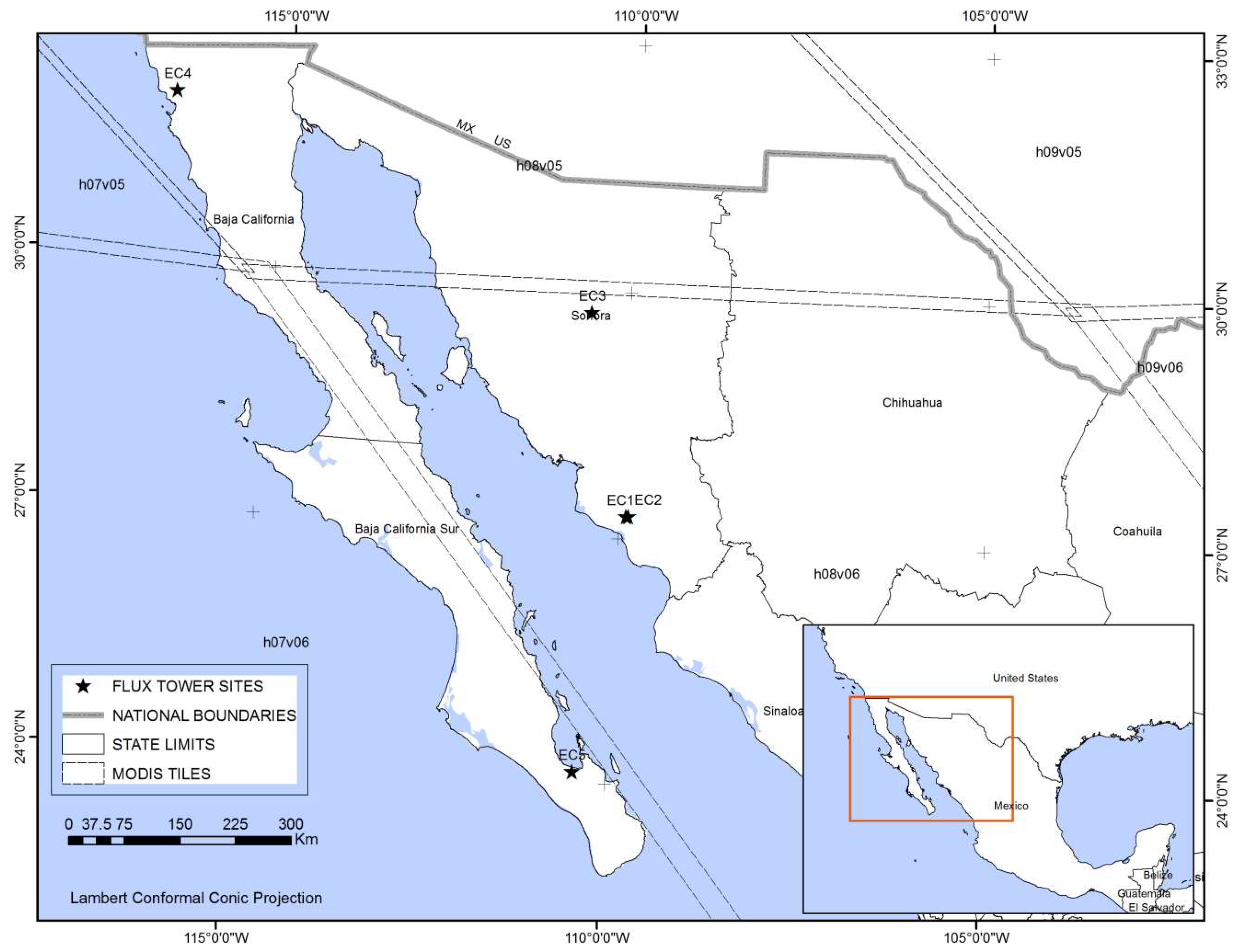
The satellite product used in this work was MOD16A2, the most recent version of MOD16 on an 8-day temporal scale (8-day average) with a spatial resolution of 500 m [56]. The images are available in the HDF-EOS format, and each image covers about 1200 × 1200 km, corresponding to the MODIS mosaics (http://modis-land.gsfc.nasa.gov/MODLAND grid.html). The study sites are within three mosaics (h08v06, h08v05 and h07v06), see Figure 1. The raster layer corresponding to the Latent heat turbulent flux (LE) variable was extracted from each MOD16A2 ET file, and the values were converted to the average ET values in mm·day⁻¹ (the 8-day average) for each pixel corresponding to the EC sites, using ArcGis 10× (https://www.esri.com/en-us/arcgis/about-arcgis/overview).

2.2. Eddy Covariance Sites

In this work, the ET estimates derived from the MOD16A2 product were compared with the ET measurements in five eddy covariance systems (EC) in northern Mexico. The location and the main characteristics of the study sites are presented in the

Table 1. Description of the sites with installation of eddy covariance system (EC): site abbreviation, site name, vegetation type, MODIS cover land (ModCL, Cshrub: Close shrub, Oshrub: Open shrub), State (Son: Sonora, BCN: Baja California Norte, BCS: Baja California Sur), Elevation (Elev, unit: m), Latitude (Lat), Longitude (Lon), mean annual precipitation (P, unit: mm), mean annual temperature (T, unit: °C), and references describing the measurements.

Site	Name	Vegetation	ModCL	State	Elev	Lat	Lon	P	T	Reference
EC1	Valle de Yaqui1	Crop: wheat	Crop	Son	36	27.278	−109.904	261	22	Rodríguez, et al. [59]
EC2	Valle de Yaqui2	Crop: wheat	Crop	Son	40	22.279	−109.873	261	22	Castañeda [58]
EC3	Rayón	Shrub	Cshrub	Son	632	29.741	−110.533	487	21	Villareal, et al. [60]
EC4	El Mogor	Shrub	Oshrub	BCN	406	32.029	−116.604	309	17	Villareal, et al. [60]
EC5	La Paz	Shrub	Oshub	BCS	21	24.129	−110.438	181.8	23.6	AmeriFlux [61]

.

EC1 and EC2 where located in the Irrigation District Valle del Yaqui [57]. The sites are located in northern Mexico (Figure 1); this zone has a semi-arid climate with summer rains (July–October), the average annual temperature is 22 °C, and the average annual precipitation is 261 mm [58]. During the experimental phase of the PLEIADeS project (Participatory Multi-Level EO-Assisted Tools for Irrigation Water Management and Agricultural Decision-Support), in the winter–spring cycle of the years 2007–2008, micro-meteorological measurements were made to determine water consumption in annual crops, including wheat (EC1 and EC2), in an area of 1600 ha. The energy balance closure was 0.82, and the heat fluxes were not corrected. For additional information about the EC systems, the reader is referred to Castañeda [58] and Rodríguez, et al. [59].

EC3 is 4 km northeast of the city of Rayón and corresponds to subtropical shrublands. The species with the highest soil cover are Fouquieria macdougalii, Parkinsonia praecox, Acacia cochiacanta, Jatropha cordata, and Encelia farinosa. It has a dry warm climate, with hot and humid summers (about 70% of rain occurs between July and September) and cold winters. The average annual temperature is 21 °C, and the average annual precipitation is 487 mm. The site is equipped with a T45 tower 9 m high that supports the eddy covariance system with an open-path infrared gas analyzer (IRGA, LI-7500, LI-COR) and a three-dimensional sonic anemometer (CSAT 3, Campbell Scientific, Logan, UT, USA). Villareal, et al. [60].

EC4 El Mogor (EC4) is located 406 m above sea level in Valle de Guadalupe, Baja California; the plants found in this site are Mediterranean shrubs; this shrubland is characterized by a mixture of chaparral, representing the most abundant species at the study site, namely, Adenostoma fasiculatum, Ornithostaphylos oppositifolia, Cneoridium dumosum, Salvia apiana, and Lothus scoparius, with less abundance of sclerophyllous plant species. It has a Mediterranean climate with hot, dry summers and cool, wet winters (November–April). The flow measurement system consisted of an open-path infrared gas analyzer (IRGA, LI-7500, LI-COR) and a three-dimensional sonic anemometer (81000V, Young, Traverse City, MI, USA) installed at 3.5 m above ground level [60]. The energy balance closure, an independent measurement to evaluate the Eddy Covariance performance, was 0.82 for the EC3 site and 0.89 for EC4 site during the years 2008 to 2010. These reports are in accordance with Fluxnet open and closed shrublands [60].

Site EC5 corresponds to one of the sites of the Ameriflux network (http://ameriflux.lbl.gov/), measuring ecosystem energy fluxes. This site is called MX-Lpa by the network. It is located 21 m above sea level, west of La Paz, within the experimental reserve of the Center for Biological Research of the Northwest (CIBNOR). The predominant vegetation is the open shrubland; the average height of the canopy is 2–3 m, with Pachycereus pringlei representing the tallest species (6–8 m). The dry desert climate of the site is characterized by variable annual precipitation, with the highest incidence of rain between August and September (182 mm year⁻¹); the average annual temperature is 23.6 °C, and the highest solar radiation occurs during the period from April to August. The flux measurement system consisted of a three-dimensional sonic anemometer–thermometer (Wind Master Pro, Gill Instruments, Lymington, UK) and an open-path gas analyzer (LI-7500, LI-COR, Lincoln, NE, USA) mounted on a tower 13 m above the surface [62]. The energy balance closure was 0.95 during the analyzed period.

For the comparison with MOD16 ET estimates, the available EC measurements were processed to obtain 8-day averages. For EC1 and EC2, the available ET values at a daily scale were used to obtain the 8-day averages for the year 2008. For EC3 and EC4 sites, there is access to the daily ET estimates for the 2008–2010 period (https://doi.org/10.3334/ORNLDAAC/1309) [60], and the 8 day- averages were processed for the whole period. For EC5, LE measurements at 30 min intervals are available for the 2004–2006 period (http://ameriflux.lbl.gov/data/download-data) [61]; these values were averaged at a daily scale, considering valid only the days (24 h period) with more than 40 data of 30 min averages. The daily averages of latent heat turbulent flux (LE) were transformed into ET values (mm·day⁻¹) using the latent heat of vaporization value of water (2.45 MJ·m⁻²) [13]. The number of 8-day average values and the period monitored are presented in

Table 2. Performance assessment of MOD16 in relation to EC, in northern Mexico based on the Root mean Square Error (RMSE), bias (BIAS), concordance index (d), and coefficient of determination (R²).

Site	Name	Year	Number of Data 1	Mean MOD16	Mean EC	RMSE	BIAS	d	R2
				mm·day−1	mm·day−1	mm·day−1	mm·day−1
EC1	Valle Yaqui	2008	15	2.76 ± 1.29	2.65 ± 0.97	0.68	0.11	0.90	0.72
EC2	Valle Yaqui	2008	8	2.65 ± 1.80	4.01 ± 1.44	1.85	−1.48	0.72	0.58
EC3	Rayón	2008	19	1.28 ± 1.06	1.85 ± 1.42	0.85	−0.57	0.88	0.93
		2009	42	0.61 ± 0.78	0.92 ± 1.09	0.58	−0.31	0.90	0.84
		2010	43	0.75 ± 0.87	1.32 ± 0.87	0.88	−0.56	0.86	0.88
EC4	El Mogor	2008	39	0.87 ± 0.41	0.85 ± 0.47	0.41	0.02	0.74	0.30
		2009	40	0.79 ± 0.31	0.88 ± 0.55	0.37	−0.09	0.79	0.60
		2010	41	1.11 ± 0.41	1.16 ± 0.51	0.38	−0.04	0.81	0.46
EC5	La Paz	2004	32	0.64 ± 0.23	0.87 ± 0.45	0.42	−0.23	0.62	0.41
		2005	34	0.53 ± 0.14	0.57 ± 0.25	0.26	−0.04	0.48	0.04
		2006	37	0.49 ± 0.24	0.76 ± 0.63	0.52	−0.27	0.65	0.69

¹ One full year of MOD 16 information consists of 45 data of the average ET (mm·8 days⁻¹).

.

2.3. Data Analyses

To evaluate the performance of MOD16 in relation to the measurements obtained by EC, four data comparison indicators were used: (1) the root of the mean square error (RMSE), measures the variation of the calculated values with respect to the observed ones; (2) the bias (BIAS), which may be positive (overestimation) or negative (underestimation), over the observed ones; (3) the concordance index (d), proposed by Willmott [63], represents the ratio of the mean square error and the potential error; (4) the coefficient of determination (R²). The first three indicators were calculated with the following equations:

$$\mathrm{RMSE}=\sqrt{\frac{\sum {(\mathrm{EC}-\mathrm{MOD}16)}^2}{\mathrm{N}}}$$

(5)

$$\mathrm{BIAS}=\frac{\sum (\mathrm{MOD}16-\mathrm{EC})}{\mathrm{N}}$$

(6)

$$\mathrm{d}=1-\frac{\sum {(\mathrm{MOD}16-\mathrm{EC})}^2}{\sum {(\left|\mathrm{EC}-\overline{\mathrm{MOD}16}\right|+\left|\mathrm{MOD}16-\overline{\mathrm{MOD}16}\right|)}^2}$$

(7)

The coefficient of determination (R²) was used as a measure of the quality of fitting, understood as the proportion of the variability explained by the fitted model (Equation (8)).

$${\mathrm{R}}^2={\lfloor \frac{\sum (\mathrm{MOD}16-\overline{\mathrm{MOD}16})(\mathrm{EC}-\overline{\mathrm{EC}})}{\sqrt{\sum {(\mathrm{MOD}16-\overline{\mathrm{MOD}16})}^2}\sqrt{\sum {(\mathrm{EC}-\overline{\mathrm{EC}})}^2}}\rfloor }^2$$

(8)

where EC is the eddy covariance-based ET at a daily scale (mm · day⁻¹); MOD16 is the ET at a daily scale (mm · day⁻¹).

3. Results

Comparison of Data Pairs

MOD16 had the best performance in the EC3 site (Table 2), for which the lowest error and the highest concordance index among the data were observed (RMSE = 0.58 mm·day⁻¹, d = 0.90). The best performance of MOD16 was evident in land with close shrub cover in comparison with land with open shrubs (EC4 and EC5) and wheat crops (EC1 and EC2) (

Table 3. Performance assessment of MOD16 in relation to EC in northern Mexico based on the Root mean Square Error (RMSE), bias (BIAS), concordance index (d), and the coefficient of determination (R²). MODIS cover land (ModCL, Cshrub: Close shrub, Oshrub: Open shrub).

ModCL	Site	Mean MOD16	Mean EC	RMSE	BIAS	d	R2
		mm·day−1	mm·day−1	mm·day−1	mm·day−1
Crop	EC1 and EC2	2.69 ± 1.45	3.13 ± 1.31	1.218	$-$0.44	0.78	0.43
Cshrub	EC3	0.79 ± 0.89	1.25 ± 1.35	0.767	−0.46	0.88	0.86
Oshrub	EC4 and EC5	0.75 ± 0.38	0.86 ± 0.52	0.401	−0.11	0.77	0.44

). In the EC5 site, a poor performance of MOD16 for the three-year study was found. For the EC1 and EC2 sites, only one-third and one-fifth of information on the 8-day periods during the year were available. The greatest deficiency according to the RMSE was observed on the site with the least number of data (RMSE = 1.85 mm·day⁻¹ EC2). Although the concordance index (d = 0.72) was acceptable, the modelled values explained only 58% of the variability (R² = 0.58), much less than in EC1, where two parameters showed better performance (d = 0.90 and R² = 0.72). In general, MOD16 underestimated the values of ET, except for EC1 and EC4 in 2008, for which the model barely overestimated the ET (BIAS = 0.11 mm·day⁻¹, BIAS = 0.02 mm·day⁻¹, respectively).

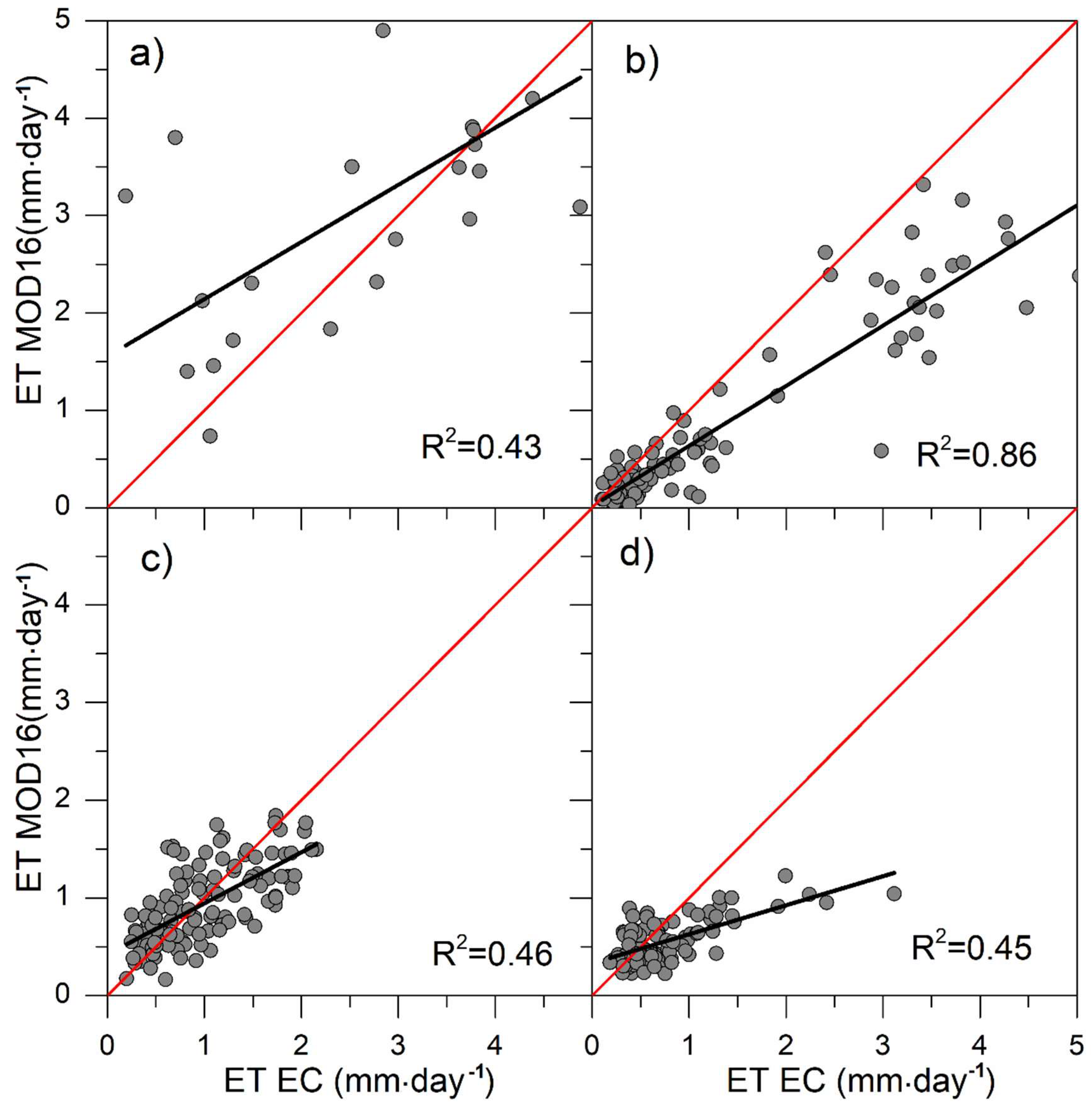
The performance of MOD16 was analyzed (Figure 2) by grouping the EC1 and EC2 sites and comparing them with EC3, EC4, and EC5 for every analyzed period. All data were considered, i.e., EC3 and EC4 for 2008–2010 and EC5 for 2004–2006. The highest concordance index and coefficient of determination (d = 0.88 and R² = 0.86) were observed in EC3, although the highest RMSE was obtained for this site (RMSE = 0.77 mm·day⁻¹). EC4 and EC5 presented errors and coefficients of determination close to each other (RMSE = 0.39 mm·day⁻¹, R² = 0.46 and RMSE = 0.42 mm·day⁻¹, R² = 0.45, respectively), although the data had a higher concordance in EC4 (d = 0.80,) than in EC5 (d = 0.62). As presented in Figure 2, the correlation between measured and modelled values indicated a clear overestimation by MOD16 under high ET rates in EC5, but the errors had not a clear tendency in EC4. The poorest performance was observed when grouping EC1 and EC2, sites covered with wheat crop (RMSE = 1.22 mm·day⁻¹, BIAS = −0.44, d = 0.78). For several 8-day averages, MOD16 overestimated ET (points below the red (1:1) line); however, the BIAS estimated for each site indicated that MOD16 underestimated the measured ET.

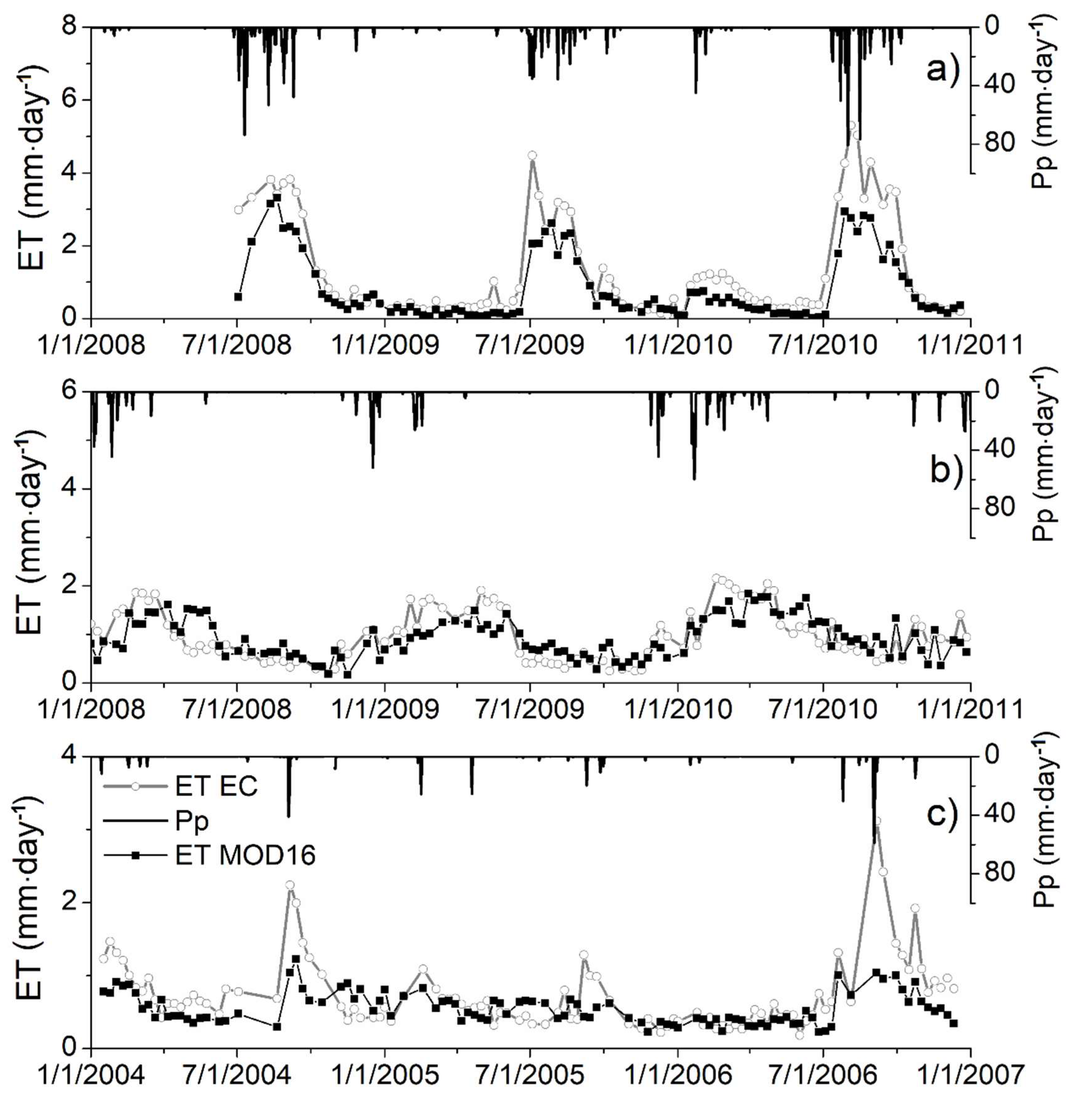
The analysis of the correlations pointed to the relative good agreement of the measured and modelled values during most of the analyzed period (see Figure 2). However, the modeled values were not able to reproduce the sudden increases of ET measured by the EC systems during the rain period in the sites with natural vegetation (EC3, EC4, and EC5). Figure 3 represents the temporal evolution of the measured values of ET and precipitation. As shown in Figure 3, the ET values changed from around 1.2 mm·day⁻¹ during winter to up to 6 mm·day⁻¹ in the site EC3 during the rainy season. In addition to the increment in the evaporation from soil and plant surfaces, plant transpiration could be increased during these periods. We interpret these data suggesting that the model based on canopy resistances does not account for the increase of the transpiration rates as a consequence of the expected increment in water availability for the plants. In addition, the simulation of soil evaporation and plant interception exclusively based on the relative humidity should be revisited according to the analyzed conditions.

4. Discussion

This study focused on the assessment of the performance of the satellite product MOD16A2 in arid zones of northern Mexico by comparing the ET values estimated by the MOD16 algorithm with the values estimated by EC systems. The ecosystem monitored corresponded to wheat crops and shrubs. Differences between both methods for ET estimation were found, which can be attributed to multiple factors associated to the generation of the algorithm [40]. In a general way, the differences can be attributed, primarily, to the parameterization of the MOD16 algorithm (inputs) and to the considerations about physical processes that influence ET, secondly, to the EC measurements, considered as “real ones”, and, thirdly, to the spatial and temporal scales of each method.

The parameterization of the MOD16 algorithm plays an important role in the accuracy of ET estimations [40]. Soil moisture has a great influence on the aerodynamic or surface resistance of the foliage and on the resistance of the soil surface, which are essential parameters in the algorithm. The ecosystem in arid and semi-arid zones is driven by moisture in the soil [64,65]; however, this is not directly considered in the algorithm [43], since it is very difficult to obtain it in a large area because of the variety of soil permeability values and associated textures [64]. However, it is possible to use available mapped information about textures in Mexico and integrate it into the MOD16 algorithm to improve it. However, and even in these conditions, the simulation of soil water content will require the integration of precipitation data that are not generally available in most areas; also, the precision of the global estimates grilled products must be analyzed. A relationship between the vapor pressure deficit (VPD) and the relative humidity (RH) is assumed [66], which is highly questionable [3] and could lead to the underestimation identified in this work. Previous model validations of MOD16 showed a similar underestimation of ET in sparse natural vegetation, such as crops [67], savanna [40], and grassland [68]. As pointed out by these authors, the differences may be due to the uncertainty of the input variables (Leaf area index (LAI) or meteorological data). These results indicate the necessity of improving the model formulation focused on the variation of canopy conductance. Identical forced models can determine what controls the accuracy of ET in our sites. It is urgent to improve strategies to measure meteorological drivers and local vegetation properties, such as relative humidity, net radiation, canopy conductance, and leaf area index, especially in the rainy season. It will be important to evaluate other satellite products with higher spatial and temporal resolution or rescale MOD16 RS inputs using another satellite products with better resolution.

In addition, the Global Modelling and Assimilation Office (GMAO) meteorological information reanalysis is validated at a global scale. It was resampled from ~110 km (0.5°) to 1 km to be inserted in the MOD16 algorithm, a process that may introduce uncertainty in the ET estimation. Other products that can introduce significant errors are the classification of coverage and land use (MOD12Q1) and LAI/FPAR (MOD15A2). Discrepancies have been found when comparing the classification of land use by the MODIS product with that made in the field [49], in contrast with this study, in which the classifications coincide both for shrublands in EC3, EC4, and EC5 and for crops in EC1 and EC2; however, MOD16 considers constant the properties for the same biome, so the phenological and structural differences of the shrubs are not captured, having an impact on the ET estimates. It has been found that when comparing MOD16 to estimates of reference evapotranspiration (ETo) in southeastern Mexico, in areas of higher humidity, there is a 0.21 coefficient of correlation, suggesting that it is necessary to parameterize the algorithm with locally derived data [50]; even though higher correlations were found in this study, it is necessary to obtain local phenology measurements, associate them with the national land cover classification, and then integrate them in MOD16.

Secondly, there are uncertainties associated with the EC measurements, which may be caused by the instrument calibration, the necessary postprocessing in the flux measurements, and the problem of closing the energy balance. For this study, EC measurements were obtained from previous studies and were considered as real ET. Authors reported energy balance closure for EC1 and EC2 (0.82), El Mogor (0.82), and Rayón (0.89). In La Paz, the energy balance closure was 0.95. All these measurements were acceptable. A fundamental requirement is to maintain a homogeneous surface without disturbance (Fetch), which is proportional to the instrument height [18]; a Fetch 100:1 is recommended and should be higher for smoother surfaces and smaller for rough surfaces. This height is unknown for sites located in areas with wheat crops; however, it has been demonstrated that with an instrument that is 2 m high, a homogeneous area of 1.5–2.5 ha can be observed depending on the direction and speed of the wind and on the atmospheric stability [68]; in the case of Rayón, which has a rough surface, with an instrument height of 9 m, a Fetch of at least 900 m is required, a requirement that is easily fulfilled because of the type of coverage; in the case of El Mogor, the height at which the measuring instrument was placed, i.e., 3.5 m, requires a Fetch of at least 350 m, and, in La Paz, the height of 13 m can easily represent a Fetch of 1300 m. The uncertainties associated with the measurements of the flux towers can influence the indicators bias, error, and coefficient of determination [43]. The advantage of having complete measurements at intervals of 8 days was evident in the improvement of the relationship between the flux towers and MOD16 in the sites with more data [7], as was observed in EC1 and EC2.

Both the magnitude and the definition of the different components of the water balance depend to a great extent on the scale [2]. There are time lags between the ET estimates for many satellite systems, especially those with high spatial resolution, where images are obtained only periodically for a specific location (8 days in the case of MODIS); therefore, evaporation from precipitation events occurring between satellite passages or the processing of the “wet” images of recent precipitation events may bias the seasonal estimates [16]. The EC estimates, used to evaluate the MOD16 algorithm, represent a homogeneous zone with a smaller surface than the spatial scale of MOD16, in the case of the wheat crop (~0.01 km²) and El Mogor (~0.1 km²) sites. Over narrow vegetation systems or small cultivation areas, satellite pixels can overlap large mixtures of vegetation types and densities. Surface temperature signals are mixed and ET recoveries are difficult to interpret [16]. MOD16 assumes an average value for a heterogeneous area, considering it as if it were a homogeneous area, inserting a bias in the information and in the comparisons with EC

5. Conclusions

In this investigation, the ET values obtained in the eddy covariance (EC) sites were compared with the satellite information estimated by the MOD16 algorithm, in five sites located in northwestern Mexico, in arid and semi-arid zones, over wheat cultivation and shrubs. Based on the results found, it can be primarily concluded that, in Mexico, evapotranspiration measurements through EC systems are scarce; the literature reports more EC sites, but the results are not available or they are hard to access; for this reason, this study only used five sites which provided sufficient and useful information for the proposed objectives. However, it is necessary to compare MOD16 with EC in zones with different environmental conditions in Mexico, before we could recommend it at national level. Secondly, acceptable results were found to consider the applicability of MOD16A2 products in areas with close shrubs, at a regional, state, and basin scale, in arid and semi-arid zones, despite the error, bias, and medium concordance indices found between EC and MOD16. Thirdly, in the current study, sufficient evidence to recommend the use of MOD16 in crops was not obtained.

References

- Allen, R.G.; Pereira, L.S.; Howell, T.A.; Jensen, M.E. Evapotranspiration information reporting: I. Factors governing measurement accuracy. Agric. Water Manag. 2011, 98, 899–920. [Google Scholar] [CrossRef]
- Wilcox, B.P.; Breshears, D.D.; Seyfried, M.S. Water balance on rangelands. In Encyclopedia of Water Science; Stewart, B.A., Howell, T.A., Eds.; Marcel Dekker, Inc.: New York, NY, USA, 2003; pp. 791–794. [Google Scholar]
- Mu, Q.; Zhao, M.; Running, S.V. Improvements to a MODIS global terrestrial evapotranspiration algorithm. Remote Sens. Environ. 2011, 115, 1781–1800. [Google Scholar] [CrossRef]
- Fisher, J.B.; Melton, F.; Middleton, E.; Hain, C.; Anderson, M.; Allen, R.; Mccabe, M.F.; Hook, S.; Baldocchi, D.; Townsend, P.A.; et al. The future of evapotranspiration: Global requirements for ecosystem functioning, carbon and climate feedbacks, agricultural management, and water resources. Water Resour. Res. 2017, 53, 2618–2626. [Google Scholar] [CrossRef] [Green Version]
- Gómez-Reyes, E.; Ponce-Palafox, J.T.; Arredondo-Figueroa, J.L.; Castillo-Vargasmachuca, S.; Benítez-Valle, A.; Ramírez-León, H. Water balance of La Yesca municipality, Nayarit, México. Rev. Bio Cienc. 2015, 3, 228–246. [Google Scholar] [CrossRef]
- Návar, J. Modelling the water balance components for the management of the watershed ‘La Rosilla’ Durango, México. AGROFAZ 2013, 1, 91–103. Available online: http://www.agrofaz.mx/wp-content/uploads/articulos/2013131VII_3.pdf (accessed on 15 January 2018).
- Ramoelo, A.; Majozi, N.; Mathieu, R.; Jovanovic, N.; Nickless, A.; Dzikiti, S. Validation of Global Evapotranspiration Product (MOD16) using Flux Tower Data in the African Savanna, South Africa. Remote Sens. 2014, 6, 7406–7423. [Google Scholar] [CrossRef] [Green Version]
- UNESCO. Methods for Water Balance Computation; Instituto de Hidrología de España: Madrid, Spain, 1981; Available online: http://unesdoc. unesco.org/images/0013/001377/137771so.pdf (accessed on 25 December 2017). (In Spanish)
- Hernández-Pérez, J.M.; Landeros-Sánchez, C.; Martínez-Dávila, J.P.; López-Romero, G.; Platas-Rosado, D.E.; Nikolskii-Gavrilov, I. Assessment of estimated real evapotranspiration andyield of sugarcane in Veracruz, Mexico. Rev. Mex. Cienc. Agríc. 2017, 8, 1013–1019. [Google Scholar] [CrossRef]
- Allen, R.G.; Pereira, L.S.; Howell, T.A.; Jensen, M.E. Evapotranspiration information reporting: II recommended documentation. Agric. Water Manag. 2011, 98, 921–929. [Google Scholar] [CrossRef]
- Jetse, D.K.; Tim, R.M.; Matthew, F.M. Estimating Land Surface Evaporation: A Review of Methods Using Remotely Sensed Surface Temperature Data. Surv. Geophys. 2008, 29, 421–469. [Google Scholar] [CrossRef]
- Zhang, K.; Kimball, J.S.; Running, S.W. A review of remote sensing based actual evapotranspiration estimation. WIREs Water 2016, 3, 834–853. [Google Scholar] [CrossRef]
- Allen, R.G.; Pereira, L.S.; Raes, D.; Smith, M. Crop Evapotranspiration: Guidelines for Computing Crop Water Requirements in United Nations FAO; Irrigation and Drainage Paper 56; FAO: Rome, Italy, 1998. [Google Scholar]
- Baldocchi, D.; Falge, E.; Gu, L. FLUXNET: A new tool to study the temporal and spatial variability of ecosystem-scale carbon dioxide, water vapor, and energy flux densities. Bull. Am. Meteorol. Soc. 2001, 477. [Google Scholar] [CrossRef]
- Bowen, I.S. The ratio of heat losses by conduction and by evaporation from any water surface. Phys. Rev. 1926, 27, 779–787. [Google Scholar] [CrossRef]
- Burba, G. Eddy Covariance Method for Scientific, Industrial, Agricultural, and Regulatory Applications: A Field Book on Measuring Ecosystem Gas Exchange and Areal Emission Rates; LI-COR Biosciences: Lincoln, NE, USA, 2013; p. 331. ISBN 978-0-615-76827-4. [Google Scholar]
- Doble, R.C.; Crosbie, R.S. Review: Current and emerging methods for catchment-scale modelling of recharge and evapotranspiration from shallow groundwater. Hydrogeol. J. 2017, 25, 3–23. [Google Scholar] [CrossRef]
- Bastiaanssen, W.G.M.; Bos, M.G. Irrigation performance indicators based on remotely sensed data: A review of literature. Irrig. Drain. Syst. 1999, 13, 291–311. [Google Scholar] [CrossRef]
- Kool, D.; Agam, N.; Lazarovitch, N.; Heitman, J.L.; Sauer, T.J.; Ben-Gal, A. A review of approaches for evapotranspiration partitioning. Agric. For. Meteorol. 2014, 184, 56–70. [Google Scholar] [CrossRef]
- Reyes-González, A.; Kjaersgaard, J.; Trooien, T.; Hay, C.; Ahiablame, L. Estimation of Crop Evapotranspiration Using Satellite Remote Sensing-based Vegetation Index. Adv. Meteorol. 2018, 2018, 1–12. [Google Scholar] [CrossRef]
- Bastiaanssen, W.G.M.; Noordman, E.J.M.; Pelgrum, H.; Davids, G.; Thoreson, B.P.; Allen, R.G. SEBAL model with remotely sensed data to improve water-resources management under actual field conditions. J. Irrig. Drain. Eng. 2005, 131, 85–93. [Google Scholar] [CrossRef]
- Allen, R.G.; Tasumi, M.; Trezza, R. Satellite-based energy balance for mapping evapotranspiration with internalized calibration (METRIC)—Model. J. Irrig. Drain. Eng. 2007, 133, 380–394. [Google Scholar] [CrossRef]
- Roerink, G.J.; Su, Z.; Menenti, M. S-SEBI: A simple remote sensing algorithm to estimate the surface energy balance. Phys. Chem. Earth B Hydrol. Oceans Atmos. 2000, 25, 147–157. [Google Scholar] [CrossRef]
- Su, Z. The surface energy balance system (SEBS) for estimation of turbulent heat fluxes. Hydrol. Earth Syst. Sci. 2002, 6, 85–99. [Google Scholar] [CrossRef]
- Anderson, M.C.; Norman, J.M.; Mecikalski, J.R.; Otkin, J.A.; Kustas, W.P. A climatological study of evapotranspiration and moisture stress across the continental United States based on thermal remote sensing: 1. Model formulation. J. Geophys. Res. Atmos. 2007, 112, D10117. [Google Scholar] [CrossRef]
- Norman, J.M.; Anderson, M.C.; Kustas, W.P.; French, A.N.; Mecikalski, J.; Torn, R.; Diak, G.R.; Schmugge, T.J.; Tanner, B.C.W. Remote sensing of surface energy fluxes at 10(1)-m pixel resolutions. Water Resour. Res. 2003, 39, 1221. [Google Scholar] [CrossRef]
- Sun, Z.G.; Wang, Q.X.; Matsushita, B.; Fukushima, T.; Ouyang, Z.; Watanabe, M. Development of a simple remote sensing evapotranspiration model (SimReSET): Algorithm and model test. J. Hydrol. 2009, 376, 476–485. [Google Scholar] [CrossRef] [Green Version]
- Miralles, D.G.; Holmes, T.R.H.; De Jeu, R.A.M.; Gash, J.H.; Meesters, A.G.C.A.; Dolman, A.J. Global land-surface evaporation estimated from satellite-based observations. Hydrol. Earth Syst. Sci. 2011, 15, 453–469. [Google Scholar] [CrossRef] [Green Version]
- Rodell, M.; Houser, P.R.; Jambor, U.; Gottschalck, J.; Mitchell, K.; Meng, C.-J.; Arsenault, K.; Cosgrove, B.; Radakovich, J.; Bosilovich, M.; et al. The Global Land Data Assimilation System. Am. Meteorol. Soc. 2004, 85, 381–394. [Google Scholar] [CrossRef] [Green Version]
- Ek, M.B.; Mitchell, K.E.; Lin, Y.; Rogers, E.; Grunmann, P.; Koren, V.; Gayno, G.; Tarpley, J.D. Implementation of Noah land surface model advances in the National Centers for Environmental Prediction operational mesoscale Eta model. J. Geophys. Res. 2003, 108, 8851. [Google Scholar] [CrossRef]
- Yin, J.; Zhan, X.; Zheng, Y.; Hain, C.R.; Ek, M.; Wen, J.; Fang, L.; Liu, J. Improving Noah land surface model performance using near real time surface albedo and green vegetation fraction. Agric. For. Meteorol. 2016, 218–219, 171–183. [Google Scholar] [CrossRef]
- Koster, R.D.; Suarez, M.J. Energy and Water Balance Calculations in the Mosaic LSM; NASA Technical Memorandum 104606; National Aeronautics and Space Administration, Goddard Space Flight Center, Laboratory for Atmospheres, Data Assimilation Office: Greenbelt, MD, USA, 1996; Volume 9, p. 76.
- Yang, R.; Cohn, S.E.; Da Silva, A.; Joiner, J.; Houser, P.R. Tangent linear analysis of the Mosaic land surface model. J. Geophys. Res. 2003, 108, 4054. [Google Scholar] [CrossRef]
- Liang, X.; Lettenmaier, D.P.; Wood, E.F.; Burges, S.J. A simple hydrologically based model of land surface water and energy fluxes for GSMs. J. Geophys. Res. 1994, 99, 14415–14428. [Google Scholar] [CrossRef]
- Liang, X.; Xie, Z. A new surface runoff parameterization with subgrid-scale soil heterogeneity for land surface models. Adv. Water Resour. 2001, 24, 1173–1193. [Google Scholar] [CrossRef]
- Xie, Z.; Yuan, F.; Duan, Q.; Zheng, J.; Liang, M.; Chen, F. Regional Parameter Estimation of the VIC Land Surface Model: Methodology and Application to River Basins in China. J. Hydrometeorol. 2007, 8, 447–468. [Google Scholar] [CrossRef]
- Dai, Y.; Zeng, X.; Dickinson, R.E.; Baker, I.; Bonan, G.B.; Bosilovich, M.G.; Denning, A.S.; Dirmeyer, P.A.; Houser, P.R.; Niu, G.; et al. The common land model. Bull. Am. Meteorol. Soc. 2003, 84, 1013–1023. [Google Scholar] [CrossRef]
- Castle, S.L.; Reager, J.T.; Thomas, B.F.; Purdy, A.J.; Lo, M.H.; Famiglietti, J.S.; Tang, Q. Remote detection of water management impacts on evapotranspiration in the Colorado River Basin. Geophys. Res. Lett. 2016, 43, 5089–5097. [Google Scholar] [CrossRef] [Green Version]
- Vishwakarma, B.; Devaraju, B.; Sneeuw, N. What Is the Spatial Resolution of grace Satellite Products for Hydrology? Remote Sens. 2018, 10, 852. [Google Scholar] [CrossRef]
- Mu, Q.; Heinsch, F.A.; Zhao, M.; Running, S.W. Development of a global evapotranspiration algorithm based on MODIS and global meteorology data. Remote Sens. Environ. 2007, 111, 519–536. [Google Scholar] [CrossRef]
- Armanius, D.E.; Fisher, J.B. Measuring water availability with limited ground data: Assessing the feasibility of an entirely remote-sensing-based hydrologic budget of the Rufiji Basin, Tanzania, using TRMM, GRACE, MODIS, SRB, and AIRS. Hydrol. Process. 2014, 28, 853–867. [Google Scholar] [CrossRef]
- López Avendaño, J.E.; Díaz Valdés, T.; Watts Thorp, C.; Rodríguez, J.C.; Velázquez Alcaráz, T.D.J.; Partida Ruvalcaba, L. Use of MODIS satellite data and energy balance to estimate evapotranspiration. Rev. Mex. Cienc. Agríc. 2017, 8, 773–784. [Google Scholar] [CrossRef]
- Di, S.C.; Li, Z.L.; Tang, R.; Wu, H.; Tang, B.H.; Lu, J. Integrating two layers of soil moisture parameters into the MOD16 algorithm to improve evapotranspiration estimations. Int. J. Remote Sens. 2015, 36, 4953–4971. [Google Scholar] [CrossRef]
- Kim, H.W.; Hwang, K.; Mu, Q.; Lee, S.O.; Choi, M. Validation of MODIS 16 Global Terrestrial Evapotranspiration Products in Various Climates and Land Cover Types in Asia. KSCE J. Civ. Eng. 2012, 16, 229–238. [Google Scholar] [CrossRef]
- Jia, Z.; Liu, S.; Xu, Z.; Chen, Y.; Zhu, M. Validation of Remotely Sensed Evapotranspiration over the Hai River Basin, China. J. Geophys. Res. 2012, 117, 2156–2202. [Google Scholar] [CrossRef]
- Yuan, W.; Liu, S.; Yu, G.; Bonnefond, J.; Chen, J.; Davis, K.; Desai, A.R.; Goldstein, A.H.; Gianelle, D.; Rossi, F.; et al. Global Estimates of Evapotranspiration and Gross Primary Production Based on MODIS and Global Meteorology Data. Remote Sens. Environ. 2010, 14, 1416–1431. [Google Scholar] [CrossRef]
- Hu, G.; Jia, L.; Menenti, M. Comparison of MOD16 and LSA-SAF MSG evapotranspiration products over Europe for 2011. Remote Sens. Environ. 2015, 156, 510–526. [Google Scholar] [CrossRef]
- Santini, A.D.; Ruhoff, A.L.; Rocha, H.R.D. Sensitivity of Modis Evapotranspiration Algorithm to Meteorological Input Data for Tropical Biomes. Available online: http://hdl.handle.net/10183/173905 (accessed on 10 February 2018).
- Ruhoff, A.L.; Paz, A.R.; Aragao, L.E.O.C.; Mu, Q.; Malhi, Y.; Collischonn, W.; Rocha, H.R.; Running, S.W. Assessment of the MODIS global evapotranspiration algorithm using eddy covariance measurements and hydrological modelling in the Rio Grande basin. Hydrol. Sci. J. 2013, 58, 1–19. [Google Scholar] [CrossRef]
- Alvarado-Barrientos, M.S.; Orozco-Medina, I. Comparison of satellite-derived potential evapotranspiration (MOD16A3) with in situ measurements from Quintana Roo, Mexico. In Proceedings of the 2016 IEEE 1er Congreso Nacional de Ciencias Geoespaciales (CNCG), Mexico City, Mexico, 7–9 December 2016. [Google Scholar] [CrossRef]
- Vargas, R.; Yépez, E.A.; Andrade, J.L.; Ángeles, G.; Arredondo, T.; Castellanos, A.E.; Delgado-Balbuena, J.; Garatuza-Payán, J.; González Del Castillo, E.; Oechel, W.; et al. Progress and opportunities for monitoring greenhouse gases fluxes in Mexican ecosystems: The MexFlux network. Atmosfera 2013, 26, 325–336. [Google Scholar] [CrossRef]
- CONABIO. Los ecosistemas terrestres. In Capital Natural de México, Volume I: Conocimiento Actual de la Biodiversidad; Challenger, A., Soberón, J., Eds.; Comisión Nacional para el Conocimiento y Uso de la Biodiversidad: Mexico City, México, 2008; pp. 87–108. ISBN 978-607-7607-03-8. [Google Scholar]
- Monteith, J.L. Evaporation and environment. Sym. Soc. Exp. Biol. 1965, 19, 205–224. [Google Scholar]
- Cleugh, H.A.; Leuning, R.; Mu, Q.; Running, S.W. Regional evaporation estimates from flux tower and MODIS satellite data. Remote Sens. Environ. 2007, 106, 285–304. [Google Scholar] [CrossRef]
- Myneni, R.B.; Knyazikhin, Y.; Privette, J.L.; Running, S.W.; Nemani, R.; Zhang, Y.; Tian, Y.; Wang, Y.; Morissette, J.T.; Glassy, J.; et al. MODIS Leaf Area Index (LAI) and Fraction of Photosynthetically Active Radiation Absorbed by Vegetation (FPAR) Product (MOD15) Algorithm Theoretical Basis Document; Department of Geography, Boston University: Boston, MA, USA, 1999; Version 4; p. 130. [Google Scholar]
- MOD16A2: MODIS/Terra Net Evapotranspiration 8-Day L4 Global 500 m SIN Grid V006. Available online: https://lpdaac.usgs.gov/dataset_discovery/modis/modis_products_table/mod16a2_v006 (accessed on 20 June 2017).
- Palacios, E.; Palacios, J.; Palacios, L. Agricultura de riego asistida con satélites. Tecnol. y Cienc. del Agua 2011, 2, 69–81. Available online: http://www.scielo.org.mx/scielo.php?script=sci_arttext&pid=S2007-24222011000200005 (accessed on 18 January 2018).
- Castañeda-Ibáñez, C.R.; Martínez-Menes, M.; Pascual-Ramírez, F.; Flores-Magdaleno, H.; Fernández-Reynoso, D.S.; Esparza-Govea, S. Estimación de coeficientes de cultivo mediante sensores remotos en el Distrito de Riego Río Yaqui, Sonora, México. Agrociencia 2015, 49, 221–232. Available online: http://www.scielo.org.mx/scielo.php?script=sci_arttext&pid=S1405-31952015000200009 (accessed on 25 November 2017).
- Rodríguez, J.; Watts, C.; Garatuza-Payan, J.; Rivera, M.; Lizárraga-Celaya, C.; Lopez, J.; Ochoa, A.; Moreno, S.; Rentería, M. Evapotranspiration and crop coefficient of banana chili pepper (Capsicum annuum L.) in the Yaqui valley, Mexico. Biotecnia 2011, 13, 28–35. [Google Scholar] [CrossRef]
- Villarreal, S.; Vargas, R.; Yepez, A.; Acosta, S.; Castro, A.; Escoto-Rodriguez, M.; Lopez, E.; Martinez-Osuna, J.; Rodriguez, J.C.; Smith, S.V.; et al. CMS: Evapotranspiration and Meteorology, Water-Limited Shrublands, Mexico, 2008–2010; ORNL DAAC: Oak Ridge, TN, USA, 2016. [Google Scholar] [CrossRef]
- Ameriflux Download Data. Available online: http://ameriflux.lbl.gov/data/download-data/ (accessed on 8 June 2016).
- Bell, T.W.; Menzer, O.; Troyo-Diequez, E.; Oechel, W.C. Carbon dioxide exchange over multiple temporal scales in an arid shrub ecosystem near La Paz, Baja California Sur, Mexico. Glob. Chang. Biol. 2012, 18, 2570–2582. [Google Scholar] [CrossRef]
- Willmott, C.J.; Ackleson, S.G.; Davis, R.E.; Feddema, J.J.; Klink, K.M.; Legates, D.R.; O’Donell, J.; Rowe, C.M. Statistics for the evaluation and comparison of models. J. Geophys. Res. 1985, 90, 8995–9005. [Google Scholar] [CrossRef]
- Makkeasorn, A.; Chang, N.B.; Beaman, M.; Wyatt, C.; Slate, C. Soil moisture estimation in a semiarid watershed using RADARSAT-1 satellite imagery and genetic programming. Water Resour. Res. 2006, 42, 1–15. [Google Scholar] [CrossRef]
- Verstraeten, W.W.; Veroustraete, F.; Feyen, J. Assessment of Evapotranspiration and Soil Moisture Content Across Different Scales of Observation. Sensors 2008, 8, 70–117. [Google Scholar] [CrossRef] [PubMed] [Green Version]
- Bouchet, R.J. Evapotranspiration réelle, évapotranspiration potentialle, signification climatique. Int. Assoc. Sci. Hydrol. Evaporat. 1963, 2, 134–142. [Google Scholar]
- Rodriguez, J. Downscaling Modis Evapotranspiration via Cokriging in Wellton-Mohawk Irrigation and Drainage District, Yuma, AZ. Ph.D. Thesis, University of Arizona, Tucson, AZ, USA, 11 March 2016. [Google Scholar]
- Chi, J.; Maureira, F.; Waldo, S.; Pressley, S.N.; Stöckle, C.O.; O’Keeffe, P.T.; Pan, W.L.; Brooks, E.S.; Huggins, D.R.; Lamb, B.K. Carbon and Water Budgets in Multiple Wheat-Based Cropping Systems in the Inland Pacific Northwest US: Comparison of CropSyst Simulations with Eddy Covariance Measurements. Front. Ecol. Evol. 2017, 5, 1–18. [Google Scholar] [CrossRef]
Figure 1.
Geographical location of the study sites and disposition of the Moderate Resolution Imaging Spectroradiometer (MODIS) mosaics that cover the territory of Mexico (MODIS mosaics are named h08v06, h08v05, and h07v06).
Figure 2.
Comparison of measured (EC) and modelled (MOD16) ET for the study sites analyzed. The red dotted line represents the 1:1 line, and the solid grey line represents the best fitting line. This panel shows the dispersion that exists between the data, MOD16 as the estimated variable (x) and EC as the real values (y), as well as the fitting line of the model and the line 1:1: (a) Valle del Yaqui (group of EC1 and EC2), (b) Rayón (EC3), (c) El Mogor (EC4), and (d) La Paz (EC5).
Figure 3.
Temporal evolution of the measured evapotranspiration (ET) using the eddy covariance systems and precipitation (Pp) in the sites (a) EC3, (b) EC4, and (c) EC5.