On the Difference of River Resistance Computation between the
k
−
ε
Model and the Mixing Length Model


1
College of Water Conservancy and Hydropower Engineering, Hohai University, Nanjing 210098, China
2
State Key Laboratory of Hydrology-Water Resources and Hydraulic Engineering, Nanjing 210098, China
3
National Engineering Research Center of Water Resources Efficient Utilization and Engineering Safety, Hohai University, Nanjing 210098, China
*
Author to whom correspondence should be addressed.
Water 2018, 10(7), 870; https://doi.org/10.3390/w10070870
Submission received: 22 May 2018
/
Revised: 21 June 2018
/
Accepted: 27 June 2018
/
Published: 29 June 2018
(This article belongs to the Section Hydraulics and Hydrodynamics)
Abstract
:River resistance characteristics, which can be reflected by the resistance factor, have an impact on flow and sediment transport. In the classical theory, Prandtl proposed the mixing length model for the simulation of the turbulence, and von Kármán established the logarithmic formula of the flow velocity distribution. Based on that, the expression of the resistance factor can be derived. With the development of the numerical technology, the model has been widely applied in the channels computation. However, for the different closure ways of the Reynolds stress in turbulence equations, the outcomes of the model and the Prandtl mixing length model are not exactly identical. In this paper, both qualitative and quantitative studies are carried out on the difference between these two models, with respect to the resistance factor. This difference is evaluated by the ratio of the resistance factor computed with the two models. The result shows that with the increment of the relative flow depth, the ratio first increases and then decreases. Moreover, it is also affected by the bed slope. Therefore, the difference should be taken into account when a comparison is made between the simulation results of the model and the classical theory of river mechanics.
1. Introduction
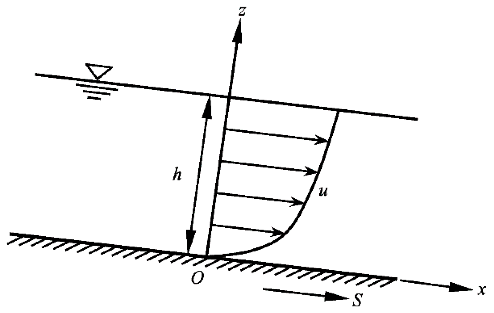
In the (vertical) two-dimensional (2D) steady uniform open channel flow, as shown in Figure 1, the vertical distribution of velocity can be expressed by the Prandtl-von Kármán logarithmic law, as follows:
where is the vertical coordinate; is the time-averaged velocity in the direction; is the shear velocity, is the bed sheer stress; is the von Kármán constant, ; is the equivalent bed-roughness and is discussed in Section 3; is the roughness function, is the roughness Reynolds number; is the kinematic viscosity coefficient. can be determined by experimental curve [1,2] or calculated approximately by the following formula [1]:
Remarkably, when , the flow is the rough turbulence, and thus ; the value is independent of . As a semi-empirical solution, Equation (1) is widely applied in the calculation of open channel flows.
The dimensionless Chézy resistance factor is defined as [1], where is the depth-averaged velocity. Considering being equal to at the relative height [1], where is the depth, the Chézy resistance factor is given by the following equation:
which is also the classical formula for .
For the two-dimensional open channel uniform flow, there exists the following equation:
where is bed slope along the channel. By combining Equations (3) with (4), can be expressed as follows:
Equation (5) is in the form of the Chézy formula, in which the dimensionless resistance factor has a relationship with the usual Chézy coefficient given by the following:
The deduction of Equation (1) relies on the closure of the Reynolds stress in turbulence equations using the Prandtl mixing length model [2] (the details on how Equation (1) is derived from the Prandtl mixing length model can be seen in [3,4]). Hence, Equation (3) is also based on the Prandtl mixing length model. However, with the development of numerical technology, the turbulence model is more widely applied than the Prandtl mixing length model. In recent years, by employing the turbulence model, Wu et al. [5] simulated the flow and sediment transport in a 180° channel bend with movable bed in the laboratory; Zhang et al. [6] developed the two-dimensional turbulence model in curvilinear coordinates to simulate the behavior of turbulent flow in an open channel partially covered with vegetation; Thi et al. [7] investigated the turbulent flow around the local scour occurring around hydraulic structures with the turbulence model. On the basis of the three-dimensional geometry model with a geological model, Wang et al. [8] presented a three-dimensional turbulence model considering Bingham liquid character. Besides these, the turbulence model is also applied in solving problems of other fields, such as air cooling technologies [9], automotive applications of on-board hydrogen storage [10], internal combustion engines scale-resolving simulation [11], pollutant removal [12], etc.
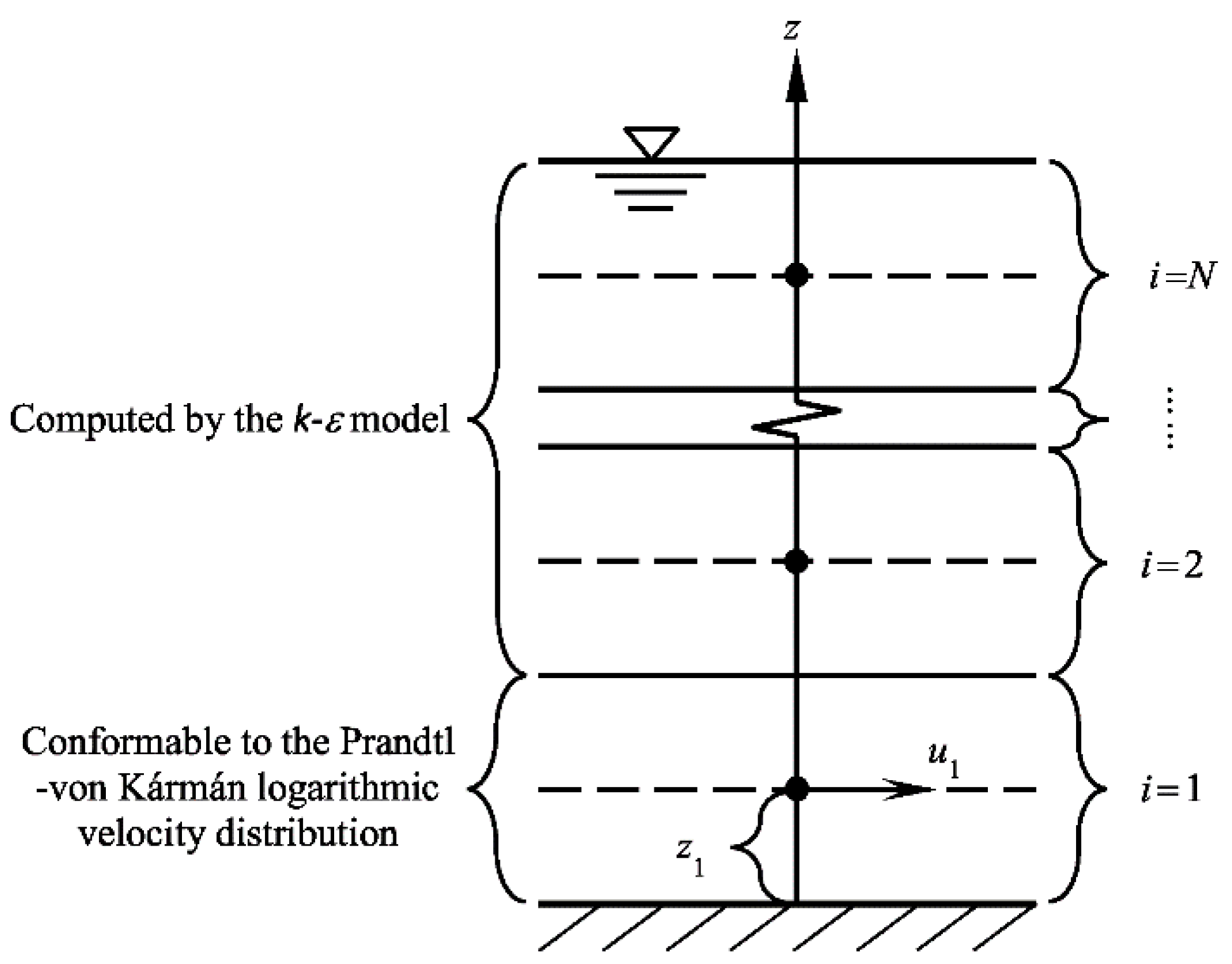
In general, the treatment of each layer in the turbulence model is shown in Figure 2, in which is the velocity near the bed; is a selected near-bed height. This treatment assumes that conforms to the Prandtl-von Kármán logarithmic law only within the range of . Above this range, however, the velocity is computed by solving the turbulence equation closed by the model. On account of that, the resistance factor corresponding to the model is not exactly identical to the one calculated by Equation (3). Note that Equation (3) is indeed the outcomes corresponding to the Prandtl mixing length model applied to the whole range of the depth. Thus, the fundamental reason causing the divergence is that there are two turbulence models using different ways in the closure of the Reynolds stress in turbulence equations. In this paper, represents the outcome of the model and represents that of the Prandtl mixing length model to distinguish them. In addition, the ratio can be regarded as the quantitative parameter measuring the difference between the two models.
In this study, the hydraulic parameters of natural rivers are collected, from which and can be computed by using the above two models. On this basis, the variation pattern of is studied.
2. Computational Methods of Resistance Factors by Using Different Models
Either way, the basic steps of computing the resistance factor are as follows:
- Solve the turbulence equations to obtain the vertical distribution of ;
- Average over the depth to obtain ; and
- Calculate the resistance factor or by the ratio of to .
Therefore, the core issue is how to solve the turbulence equations. The solving methods using the Prandtl mixing length model and the model are given separately in the below.
2.1. Prandtl Mixing Length Model
As stated in the introduction, solving the turbulence equations closed by the Prandtl mixing length model actually gives the Prandtl-von Kármán logarithmic distribution of (i.e., Equation (1)
in Section 1), which is in the continuous form. After integrating this equation, it can be identified that is
at the relative height . For that, Equation (3) is used to compute in this paper.
2.2. Model
Generally, a continuous form of velocity distribution cannot be obtained by closing and solving the turbulence equation with the model; thus, the discrete method is used. On the conditions of the two-dimensional uniform flow in open channels, the RANS (Reynolds-averaged Navier–Stokes) equation in the direction [2] can be simplified into the following:
where, and are the fluctuant velocity components in and directions, respectively; denotes the time-averaged value of the content within the angle brackets, and thus actually denotes the Reynolds stress per unit mass.
According to the Boussinesq hypothesis, for the turbulent flow, is defined as the eddy viscosity. Reynolds stress has a relationship with the time-averaged velocity gradient given by the following:
Then, Equation (7) can be transferred to the following:
Equation (9) is just the basic equation for the computation of by using the model. Then, the finite volume method is adopted to discretize this equation.
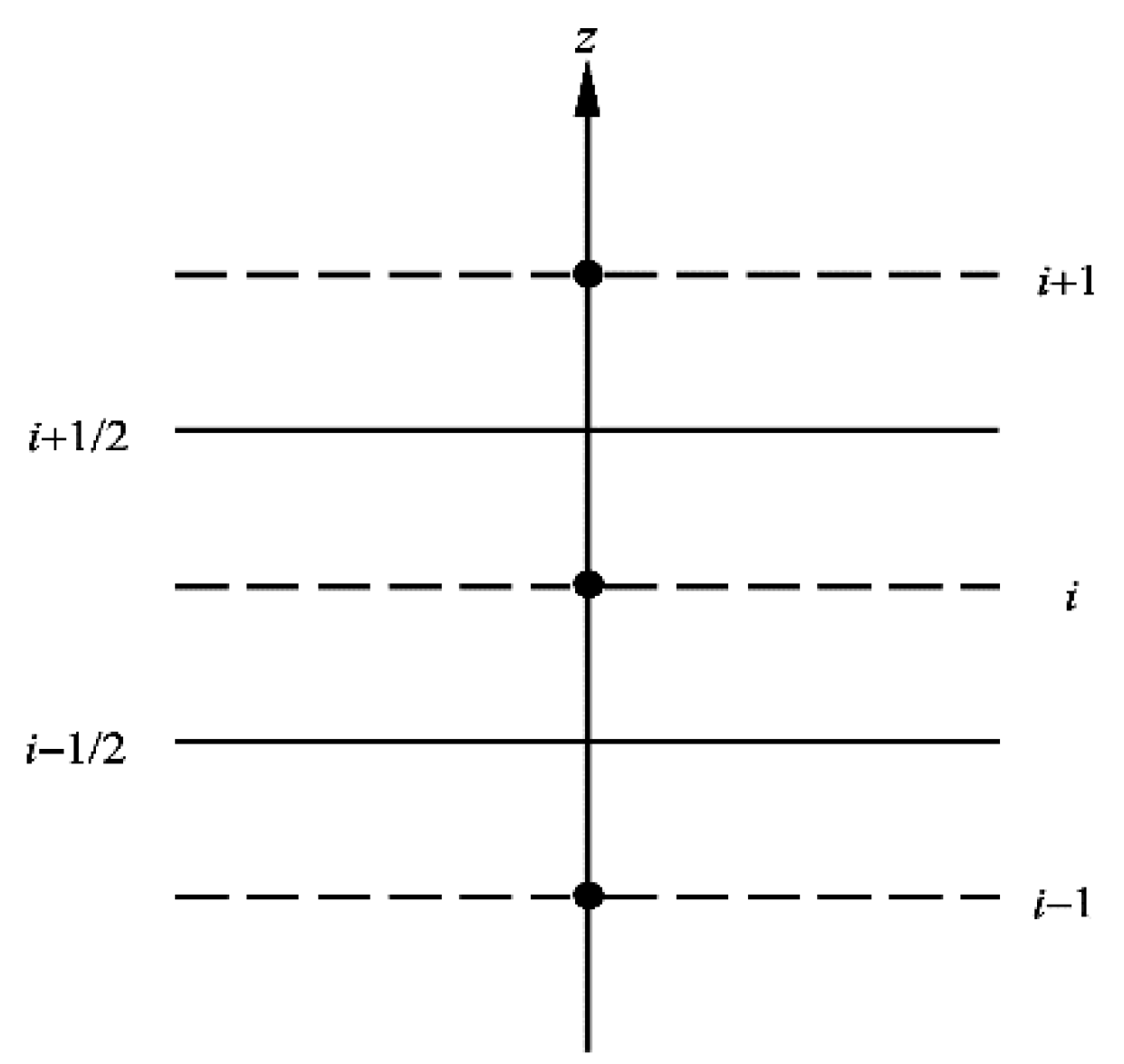
The integral of Equation (10) on the grid of the i-th layer, as shown in Figure 3, gives the following:
In which the differential terms can be further discretized with the central differencing scheme, as follows:
The substitution of Equations (11) and (12) into Equation (10) gives the following:
which is the general discrete form of Equation (9).
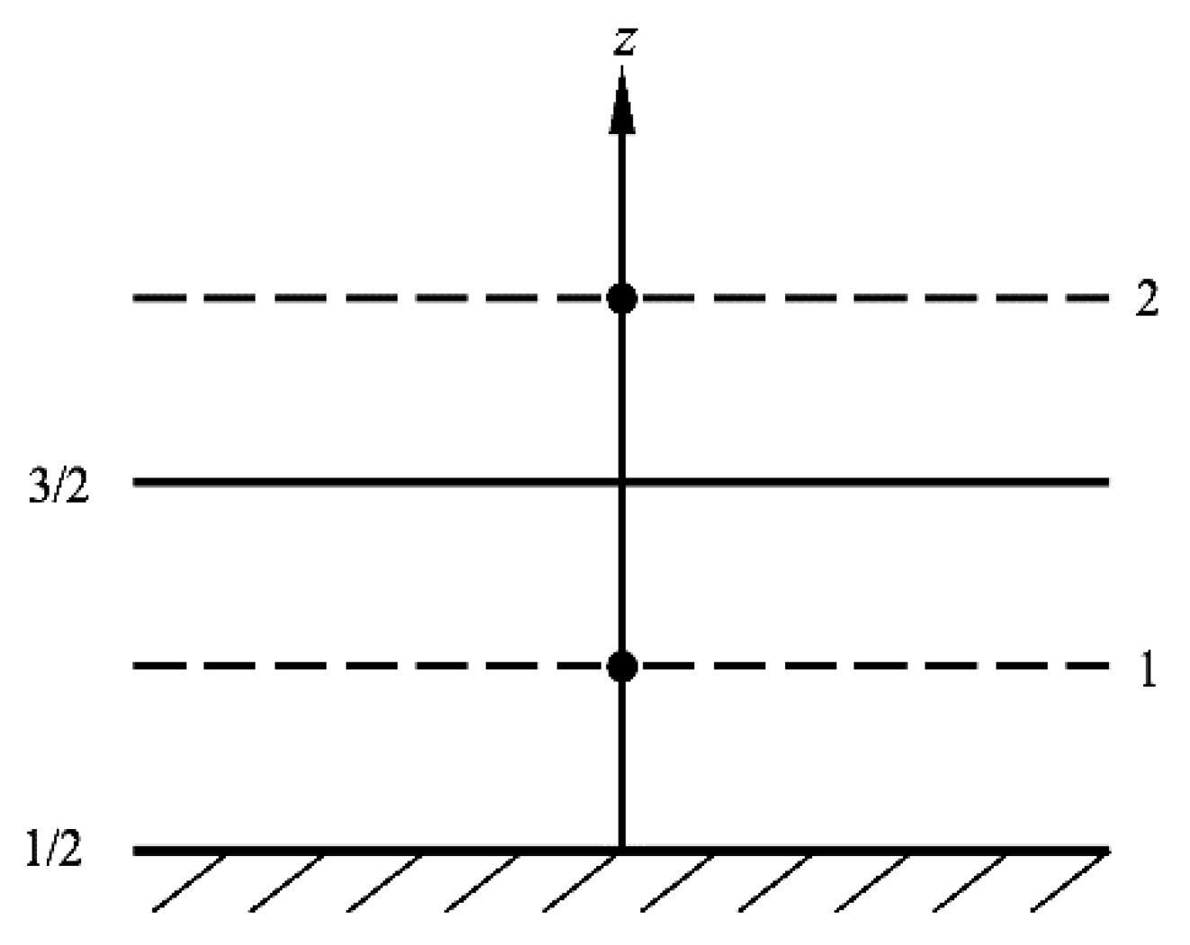
As shown in Figure 4, for the situation that , Equation (10) is transferred to the following:
The derivative term in the first term on the right-hand side can be discretized with the central differencing scheme as follows:
According to the bed boundary condition, the second term on the right-hand side can be calculated as follows:
Substituting Equations (15) and (16) into Equation (14), one obtains the following:
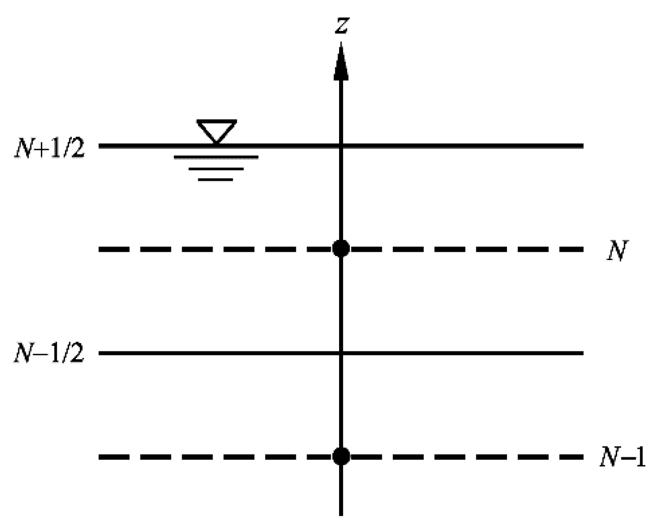
As shown in Figure 5, for the situation that , Equation (10) is transferred to the following:
The derivative term in the second term on the right-hand side can be discretized with the center difference scheme as follows:
According to the free surface boundary condition, the first term on the right-hand side can be calculated as follows:
Substituting Equations (19) and (20) into Equation (18), one obtains the following:
For the value of , at the interface of the grid, the linear interpolation is resorted to the following:
whereas the value of at the center of the grid is calculated by the model, as follows:
where is the turbulent kinetic energy; is the dissipation rate; , is the production term; the standard values of the model coefficients are employed [5,13]: 0.09, 1.0, = 1.3, = 1.44, = 1.92. Equations (25) and (26) are both differential equations, and they are discretized with the same scheme as Equation (9). In addition, for Equations (25) and (26), the bed boundary conditions [5] are as follows:
and the free surface boundary conditions [5] are as follows:
Combing Equation (13) with Equations (17) and (21), the following tridiagonal linear system is finally derived, as follows:
where,
However, the determinant of the coefficient matrix of this system turns out to be zero and the rank is (, non-full rank), which means that there exists infinitely many solutions to this system. Furthermore, this system is derived as follows.
By means of accumulative summation from the top to the bottom, Equations (29) can be transferred to the following:
The last equation of Equations (30) is as follows:
Note that . Then, after transposition, Equation (31) can be transferred to
which is the same equation as Equation (4).
From Equations (30), it follows that only the difference between the velocities of any two adjacent points can be solved. Thus, in order to get the absolute value of the velocity, another supplementary equation is needed. As stated in the introduction, it is generally assumed that the near-bed velocity within the range of () [4,14] conforms to the Prandtl-von Kármán logarithmic law, which means the following:
Then, the velocity
(i = 1, 2, …, N) of any point can be obtained by successively solving Equation (33), and then Equations (30) from the top to the bottom. The depth-averaged velocity can be evaluated as follows:
Thus, the resistance factor can be evaluated as .
The above calculation still needs iteration for in the coefficient matrix of Equations (30), involving , which is determined by the differential Equations (25) and (26).
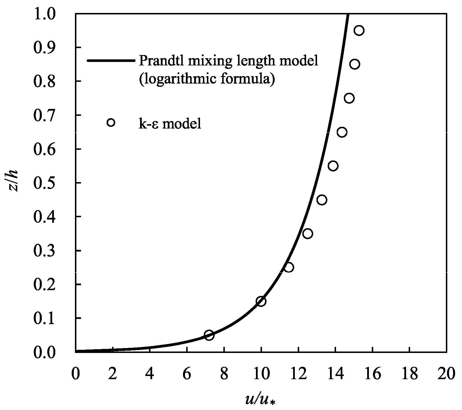
The computation methods of using the Prandtl mixing length model and the model are given, as above. Figure 6 shows the typical computations of velocity distribution by using these two models. The parameters of the Rio Grande River [15] are used in both computations: 0.332 m, 0.028 m, and 0.830 × 10⁻³. The result corresponding to Prandtl mixing length model, which is calculated by Equation (1), is shown in the continuous form; in contrast, the result corresponding to the model, which is calculated by dividing the whole depth into ten layers, is shown in the discrete form. From Figure 6, an approximate coincidence can be detected between the two velocity distribution pattern computed by different models within the range of ; however, the difference displays, to some extent, within the range of . Indeed, the Prandtl mixing length model and the model treat the shear force between the flow layers in different ways. This is the main reason the resistance factors computed with these two models are not identical.
3. Determination of Equivalent Bed-Roughness
In natural rivers, bed forms are induced by sediment transport. This means that the bed resistance to flow includes not only the grain resistance, but also the bed-form resistance—For some special cases, the resistance of other factors (e.g., the emergent vegetation) should also be taken into account [16], but they are not considered in this study. In this study, the van Rijn method [17] is employed to determine , which takes the influence of these two kinds of resistance into consideration.
The expression of proposed by van Rijn [17] is as follows:
where is the characteristic bed material diameter; and are the bed-form height and the bed-form steepness, respectively, which are determined as follows:
where is a transport stage parameter,
where is the bed shear stress related to grains; is the critical bed-shear stress for initiation of motion of grains, which can be determined by experimental curve [1,18] or calculated approximately by the following formula:
where is the dimensionless material number, which is defined as the following:
where is the density of the bed material, 2650 kg/m3; is the density of water, 1000 kg/m3.
In the work of van Rijn [17], was identified with ; in this study, however, as a result of the lack of information of reported in the references, is thus identified from all the available data within a range of ∼. Practices have indicated that although the exact value of varies with the selected, the pattern of versus does not change in a noticeable manner. This is further discussed and evidenced in Section 5.1.
4. Data, Results, and Analyses
4.1. Data Sources and Range
4.2. Analysis of Influential Factors
, and are selected as the basic dimensionally independent variables that represent the dynamic, kinematic, and geometric characteristics, respectively. Then, the Buckingham theorem is employed for the dimensional analysis. One determines for that is influenced by the following four dimensionless parameters:
within these parameters, is considered as constant (=2.65) in this paper. Thus, the influence of is not considered in the following analyses.
The product of , and gives the following:
where is the grain size Reynolds number. According to Equation (35), the roughness Reynolds number can be expressed as follows:
Here, , which is defined as the bed-form Reynolds number. According to Equation (44), is included in . Also, note that only appears in the roughness function in Equations (3) and (33). For the data of natural rivers collected in this study, it can be proved that , meaning that the flow is an invariably rough turbulent, for which ; as a consequence, in this study, is independent of and thus . Then, the influence of is neglected.
In the final analysis, is a function solely depending on and , for which one can write the following:
Note that is referred to as the relative water depth [1]. The function form of will be determined in the following subsection.
4.3. Computational Results and Analyses
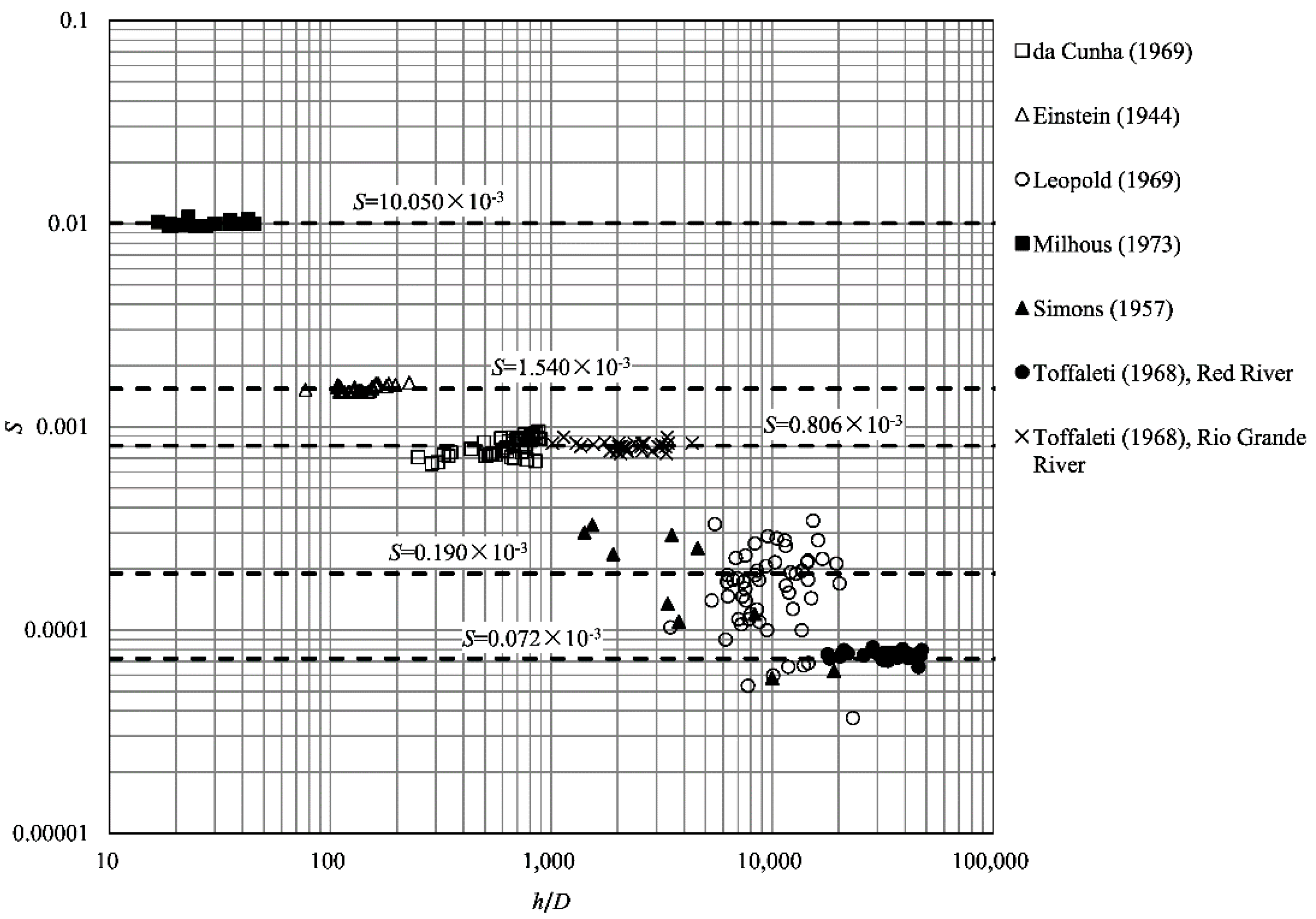
First, by clustering the data of and corresponding to all the collected natural rivers, the relation of versus is plotted in Figure 7 with log−log axes. From Figure 7, it can be seen that all the points are approximately distributed around the following five horizontal lines: 10.050 × 10⁻³, 1.540 × 10⁻³, 0.806 × 10⁻³, 0.190 × 10⁻³, and 0.072 × 10⁻³. Note that despite a considerable scatter, the points around 0.190 × 10⁻³ still follow this pattern. Thus, a classification will be made in the following contents for all the collected natural rivers on the basis of these five values of .
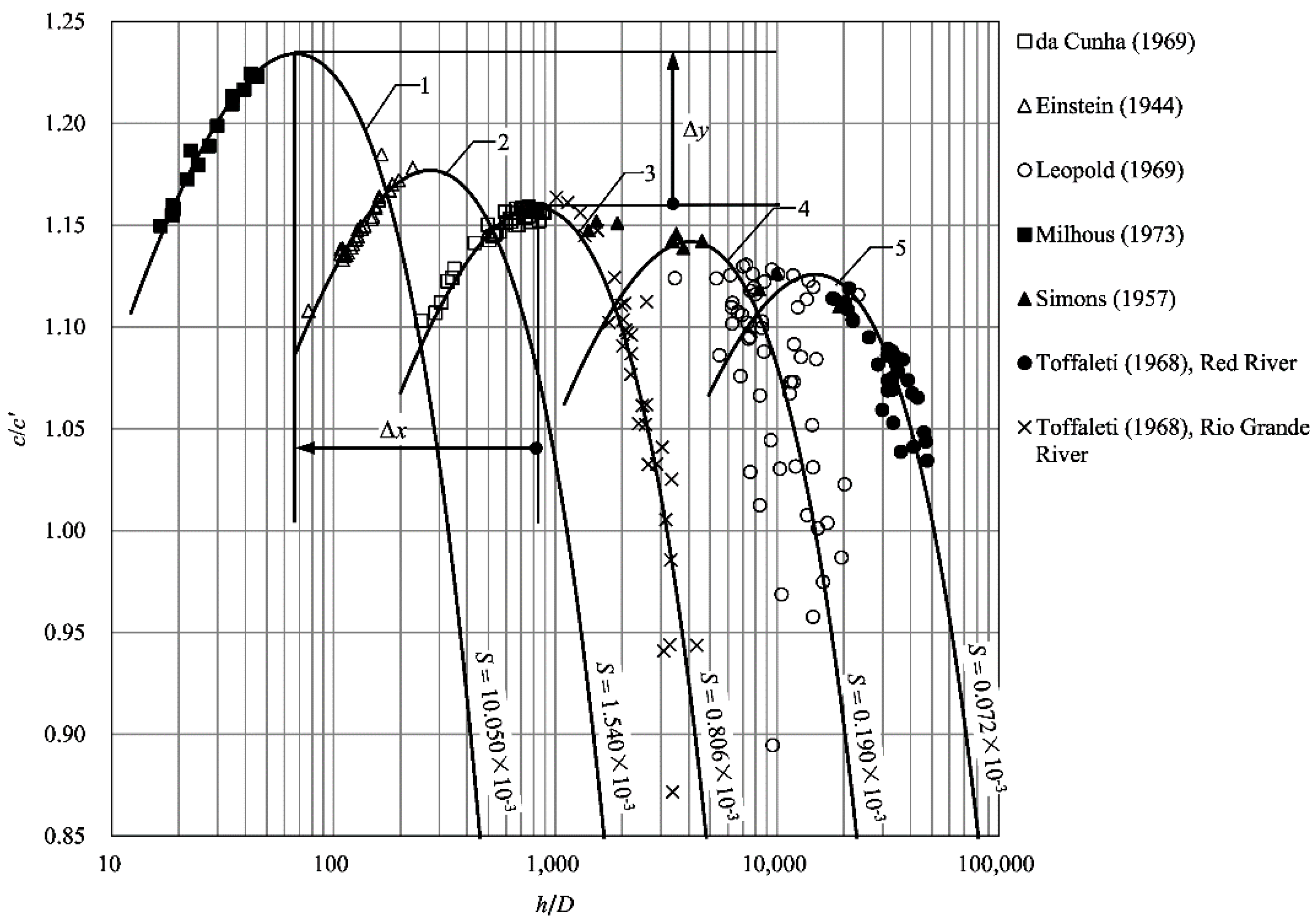
Then, with the values of corresponding to all the collected natural rivers computed, the variation pattern of versus is plotted in Figure 8 with lin−log axes. As shown in Figure 8, all the points can be classified into five groups, according to different values of , as specified above; each group is represented by a continuous curve. Although the points around curve 4 ( 0.190 × 10⁻³) are scattered, the general pattern can still be followed. With the increment of , only the points around curve 3 show a trend of ascending followed by descending, which is considered to be ‘complete’. In contrast, the points around curve 1 ( 10.050 × 10⁻³) only compose an ascending part, and so do those around curve 2 ( 1.540 × 10⁻³); the points around curve 4 ( 0.190 × 10⁻³) only compose a descending part, and so do those around curve 5 ( 0.072 × 10⁻³). Despite insufficient evidence, it can be inferred that the points around each of these five curves should have the same trend. It is due to the limited range of data that the points around each of curves 1, 2, 4, and 5 cannot show a trend as ‘complete’ as those around curve 3.
The ‘complete’ curve 3 can be approximately expressed by fitting the points around it as follows:
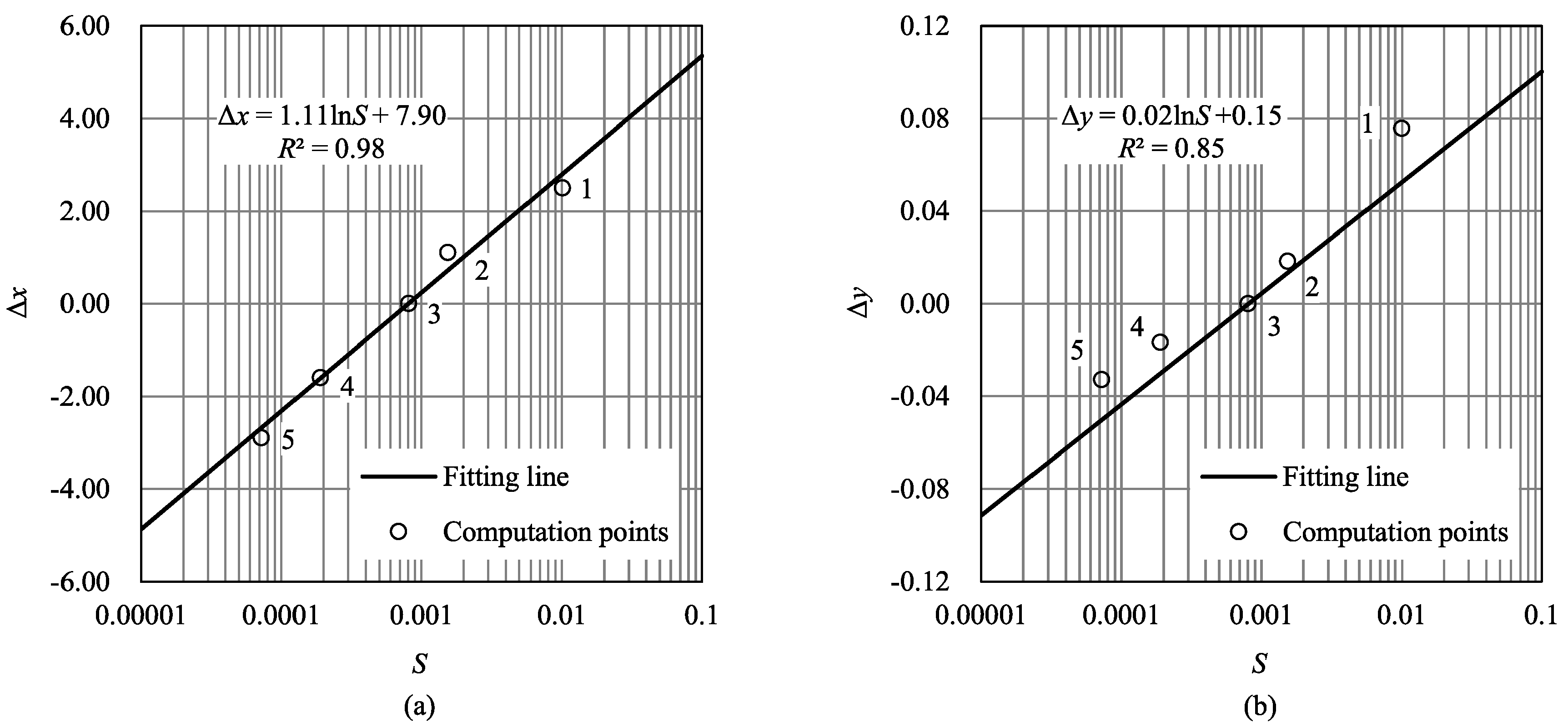
It is assumed that curves 1, 2, 4, and 5 can be obtained by translating curve 3 on the plane. Thus, two translation parameters and (see Figure 8) are introduced into Equation (46), which yields the following:
Apparently, both of and should be functions of S.
The values of and for curves 1, 2, 4, and 5 can be obtained by fitting Equation (47) to the corresponding points. Taking also into account and for curve 3, the relations of versus , and versus are plotted in Figure 9a,b, respectively, with lin−log axes. It is indicated that both and are linear with the logarithm of (). With the premise that the fitting lines pass through the points corresponding to curve 3 in Figure 8, the fitting equations are constructed as follows:
The substitution of Equations (48) and (49) into Equation (47) yields the following:
This is the functional form sought for . Note that there exists a vertical asymptote on the right side of each ∼ curve, as follows:
Thus, Equation (51) is only applicable to the following:
According to Equation (50), together with all the curves in Figure 8, the following aspects can be summarized:
- (a)
- For a specific , first increases and then decreases with the increment of ; the variation pattern of versus is shown as a convex upward curve;
- (b)
- The peak value of the convex upward curve increases with the increment of ; Figure 9b, along with Equation (49), indicates that the peak value is approximately linear with ; and
- (c)
- The abscissa of the peak value decreases with the increment of ; Figure 9a, along with Equation (48), indicates that the abscissa of the peak value is approximately linear with as well.
Moreover, from the points in Figure 8, it follows that the values of are generally greater than unity. This means that for the collected natural rivers, the resistance factors computed with the model are generally greater than those computed with the Prandtl mixing length model. However, it cannot be ignored that the circumstances where the values of are smaller than unity can also be detected, as long as the corresponding values of are sufficiently large (see Figure 8, the points on the lower right sides of curves 3 and 4).
In practice, if the data collected in a natural river include the water depth , the bed slope , and the characteristic bed material diameter , all of which satisfy Equation (52), then the flow discharge corresponding to the turbulence model can be simply calculated with the following steps, instead of by running a complex numerical model:
- Calculate the resistance factor corresponding to the Prandtl mixing length model by employing Equation (3) (see Section 2.1);
- Covert the resistance factor from the one corresponding to the Prandtl mixing length model into the one corresponding to the model by employing Equation (50);
- Substitute instead of into Equation (5) to calculate the depth-averaged velocity ; and
- Calculate the flow discharge as .
4.4. Discharge Verification
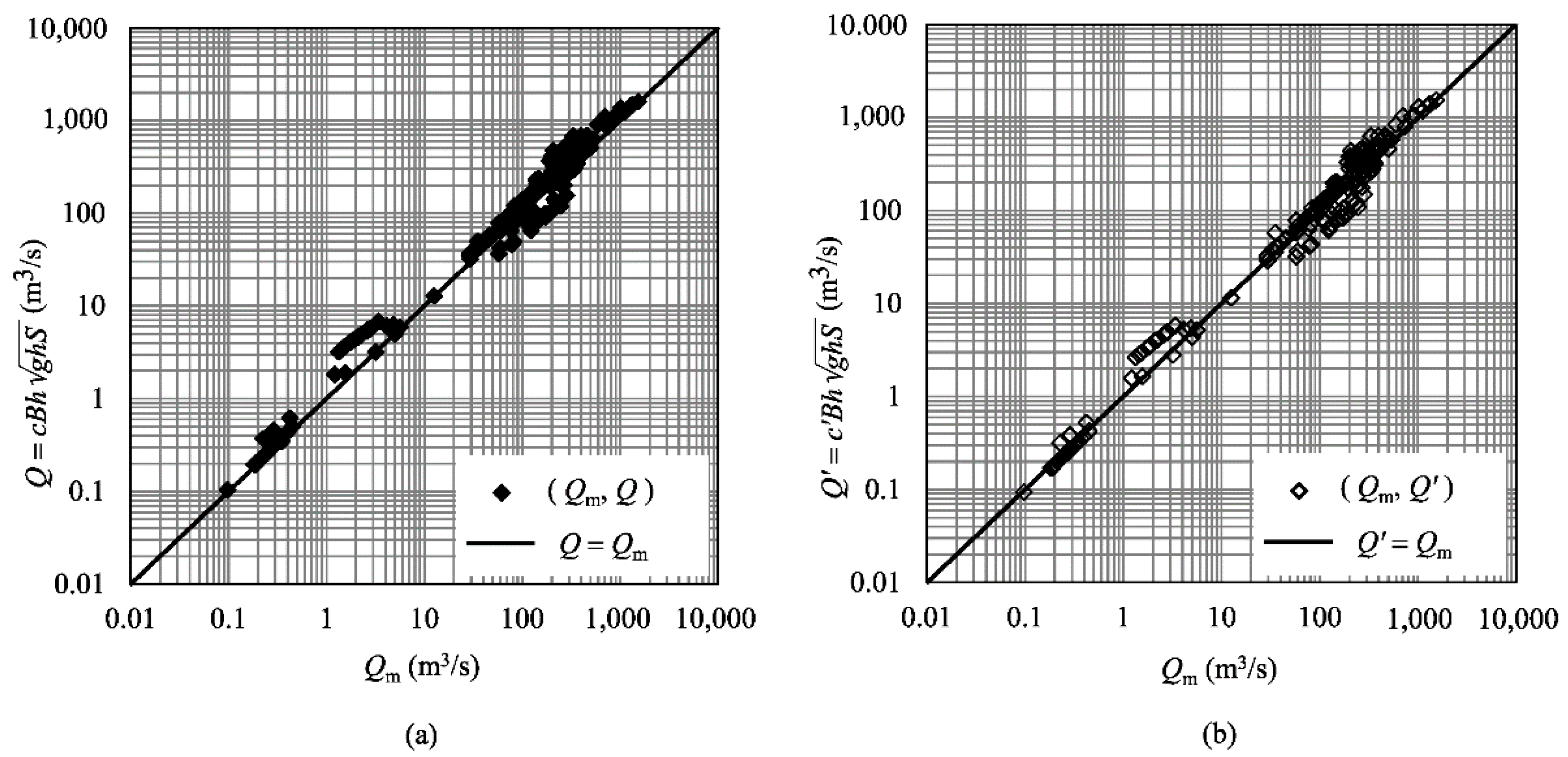
The computed flow discharge and corresponding to the model and the Prandtl mixing length model, respectively, are verified by comparing them with the field-measured flow discharge . The results are shown in Figure 10. It can be seen that both the and sets of points are evenly distributed around the line .
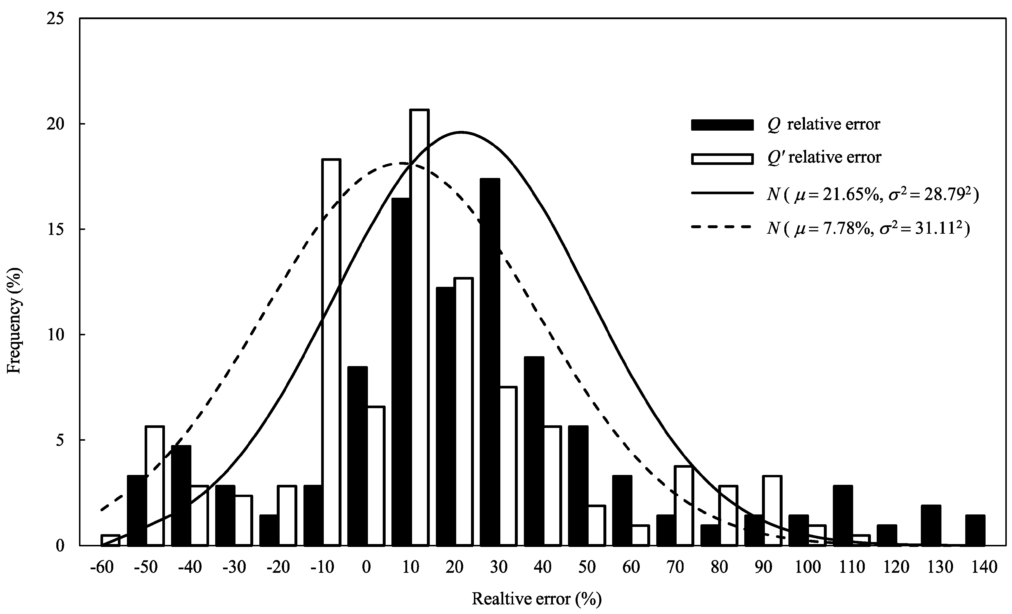
Furthermore, the frequency distributions of the computational errors of and relative to are shown in Figure 11. Both approximately conform to the normal distribution as follows:
where is the normal distribution; is the mathematical expectation of normal distribution; and is the variance.
From the values of in Equations (53) and (54), the mean relative errors of and are 21.65% and 7.78%, respectively. This means that the points in Figure 10b are closer to the line than the points in Figure 10a. From the values σ2 of in Equations (53) and (54), the variance of the relative errors of and are 28.792 and 31.112, respectively. This means that the points in Figure 10b are more scattered than the points in Figure 10a. Therefore, each of two turbulence models has its own advantages and disadvantages, if considered from different aspects.
Considering the function proposed in Section 4.3, which quantitatively describes the difference between two turbulence models in the computation of river resistance, and corresponding to the model and the Prandtl mixing length model, respectively, seem interconvertible, as follows:
As above, it is further indicated that the simulation results corresponding to the model and the Prandtl mixing length model are not identical. When comparing them, the difference between the river resistance characteristics reflected by these two models should be taken into account.
5. Discussion
5.1. Influence of the Selection of the Characteristic Bed Material Diameter
As stated in Section 3, the calculation of the equivalent bed-roughness involves a certain characteristic bed material diameter D. In this study, the available data of D are within a range of D50∼D90. Indeed, with regards to Figure 8, even though the a different type of D is selected for each point, the same trend of the computed curves can still be obtained. The points are still distributed around the same one out of the five curves, although positioned at different positions.
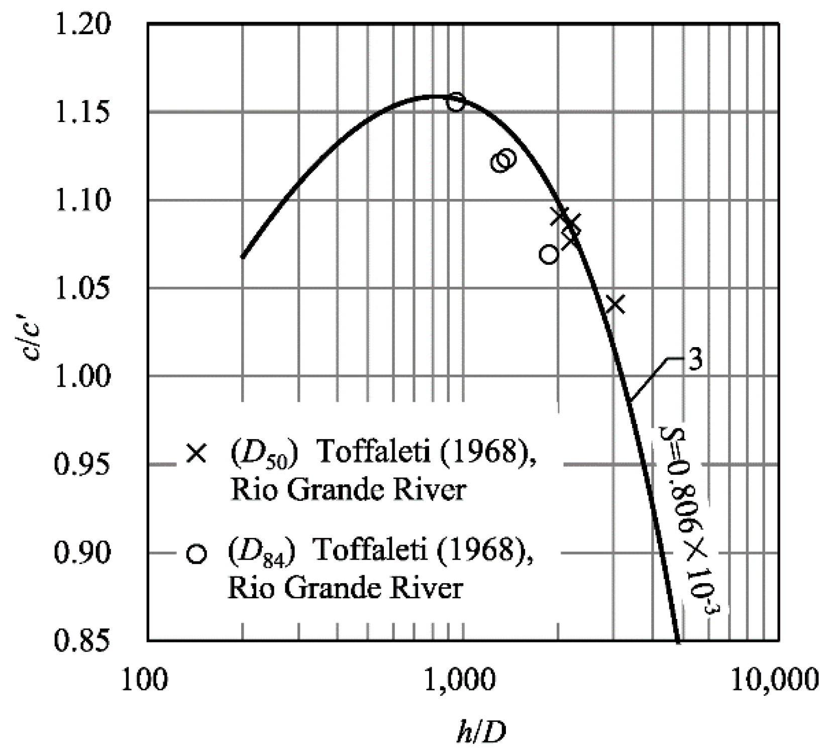
Only a few references report various types of D for a certain river; (e.g., from Rio Grande River [15]) four groups of data corresponding to different river reaches of both D50 and D84 can be extracted. In Figure 8, the points corresponding to these river reaches are computed with D50; these points, together with curve 3, which they are fitted to, are replotted in Figure 12. To show the influence of the selection of the type of D, the values of corresponding to the same river reaches are further recomputed with D84, and the corresponding points are plotted in Figure 12, too. It can be seen from Figure 12 that the points computed with D84 are also distributed around curve 3. The pattern of versus does not change in a noticeable manner if a different type of D is selected.
5.2. Influence of the Coefficients in the Model
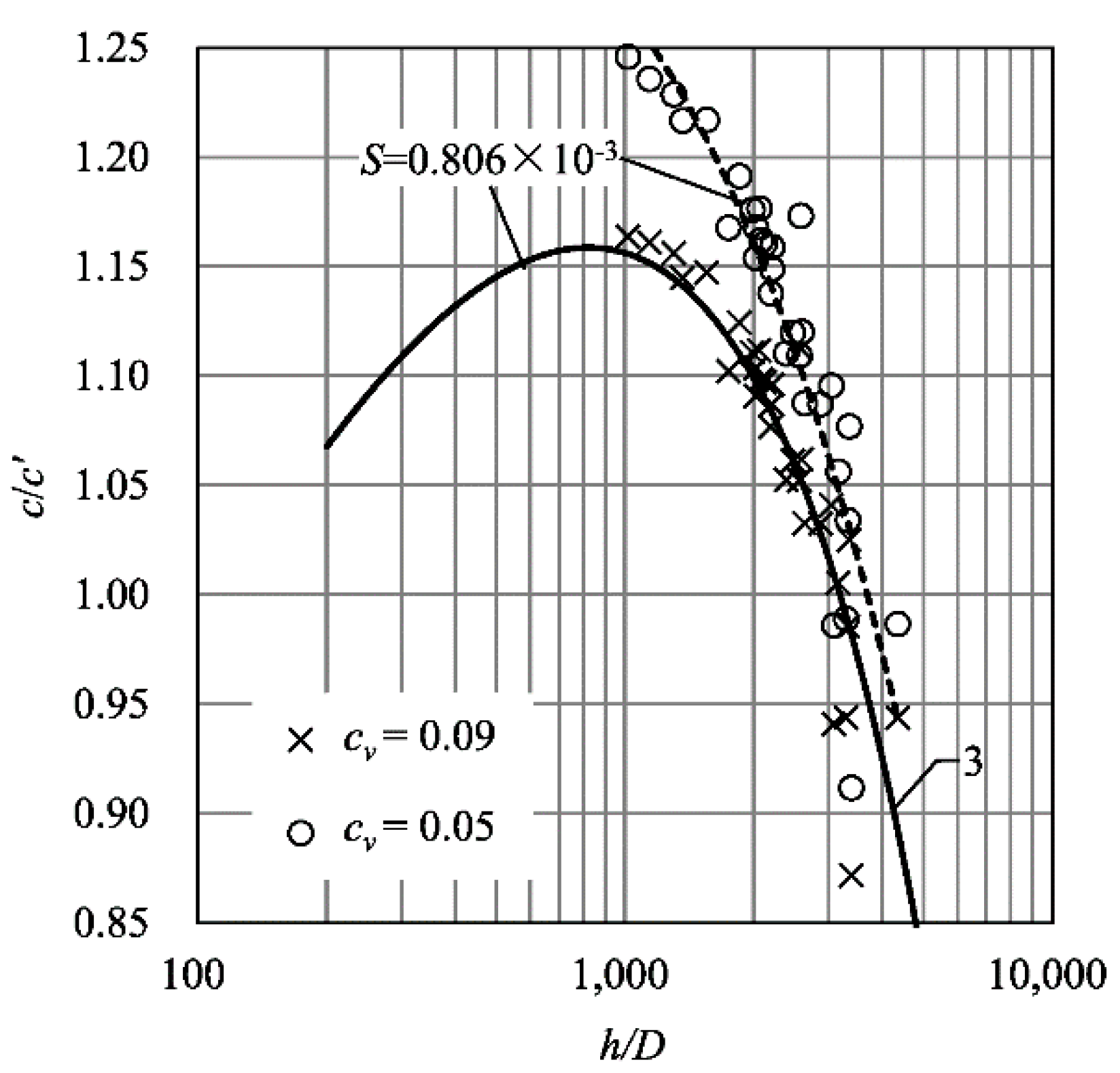
As stated in Section 2.2, the turbulence model involves five coefficients and their standard values are used, namely, 0.09, 1.0, 1.3, 1.44, and 1.92. However, according to Rodi [13], in a case where the
production of the turbulence kinetic energy is much larger than its
dissipation, the value of can be as small
as about 0.05. Figure 13 displays a partial result of
versus , with different values of : 0.09 and 0.05. From Figure 13, it follows that the computed values of with 0.05 are somewhat larger than those with 0.09. Consequently, the result presented
in this paper still depends on the values of in the model. Nevertheless, it should also be noted that with either value of , appears invariably as a function of ; that is, it can never be constant.
For lack of knowledge on how the other coefficients change according to different cases, their influences are not included in this paper. How these coefficients, including , affect the resistance factor ratio needs further studies.
6. Conclusions
With the data of natural rivers, the computational results corresponding to the model and the Prandtl mixing length model are compared and analyzed. The following has been suggested:
- (a)
- The resistance factors corresponding to these two models are not identical. A new expression Equation (50), has been derived to quantify it. The difference of these two models, evaluated by the ratio , first increases and then decreases with the increment of the relative water depth . This variation pattern can be represented by a convex upward curve, of which the peak value increases and the abscissa of the peak value decreases with the increment of the bed slope .
- (b)
- Both turbulence models can generate reasonable results with acceptable errors with respect to the flow discharges in natural rivers. Each model has its own advantages and disadvantages. Within the range of the collected natural rivers, the mean relative error of the computed flow discharges corresponding to the Prandtl mixing length model is less than that corresponding to the model; in contrast, the error distribution corresponding to the former is more scattered than that corresponding to the latter. Furthermore, the flow discharges computed with these two models can be converted into each other by taking into account Equation (55).
- (c)
- The velocity distribution patterns corresponding to these two models within the range of are approximately consistent, whereas the difference displays to some extent within the range of .
- (d)
- For river computation issues, the simulation results corresponding to the model and the Prandtl mixing length model are not exactly identical, although both can well simulate the flow. Accounting for that, the difference between the river resistance characteristics reflected by these two models should be considered.
Author Contributions
W.D. carried out the research, including framing the scope of the work and writing the manuscript. M.D. computed the data with models and analyzed the results. H.Z. provided technical supports of models and review the manuscript.
Funding
This research was funded by the National Key R&D Program of China (2016YFC0402501), the NSFC (51479071), the 111 project (B12032, B17015), the Priority Academic Program Development of Jiangsu Higher Education Institutions (3014-SYS1401), and the College Students’ Innovation and Entrepreneurship Training Program Project of Hohai University (201710294016-Zingming He, 2017102941059-Xiaoting Wang).
Acknowledgments
The authors would like to acknowledge Ishwar Joshi and Chaoyang Dai for their help of reviewing the paper.
Conflicts of Interest
The authors declare no conflict of interests.
References
- Yalin, M.S.; da Silva, A.M.F. Fluvial Process; International Association of Hydraulic Engineering and Research (IAHR): Delft, The Netherlands, 2001. [Google Scholar]
- Zhang, Z.X.; Dong, Z.N. Viscous Fluid Mechanics, 2nd ed.; Tsinghua University Press: Beijing, China, 2011. (In Chinese) [Google Scholar]
- Yalin, M.S. Mechanics of Sediment Transport; Pergamon: Oxford, UK, 1972. [Google Scholar]
- Nezu, I.; Nakagawa, H. Turbulence in Open-Channel Flows; A.A. Balkema: Rotterdam, The Netherlands, 1993. [Google Scholar]
- Wu, W.; Rodi, W.; Wenka, T. 3D numerical modeling of flow and sediment transport in open channels. J. Hydraul. Eng. 2000, 126, 4–15. [Google Scholar] [CrossRef]
- Zhang, M.L.; Shen, Y.M.; Zhu, L.Y. Depth-averaged two-dimensional numerical simulation for curved open channels with vegetation. J. Hydraul. Eng. 2008, 39, 794–800. (In Chinese) [Google Scholar]
- Thi, H.T.N.; Jungkyu, A.; Sung, W.P. Numerical and physical investigation of the performance of turbulence modeling schemes around a scour hole downstream of a fixed bed protection. Water 2018, 10, 103. [Google Scholar] [CrossRef]
- Wang, X.L.; Wang, Q.S.; Zhou, Z.Y.; Ao, X.F. Three-dimensional turbulent numerical simulation of Bingham fluid in the goaf grouting of the south-to-north water transfer project. J. Hydraul. Eng. 2013, 44, 1295–1302. (In Chinese) [Google Scholar]
- Wibron, E.; Ljung, A.-L.; Lundström, T.S. Computational fluid dynamics modeling and validating experiments of airflow in a data center. Energies 2018, 11, 644. [Google Scholar] [CrossRef]
- Wookyung, K.; Volodymyr, S.; Dmitriy, M.; Vladimir, M. Simulations of blastwave and fireball occurring due to rupture of high-pressure hydrogen tank. Safety 2017, 3, 16. [Google Scholar] [CrossRef]
- Vesselin, K.K.; Luca, S.; Giacomo, F. A modified version of the RNG k–ε turbulence model for the scale-resolving simulation of internal combustion engines. Energies 2018, 10, 2116. [Google Scholar] [CrossRef]
- Liu, F.; Qian, H.; Zheng, X.; Zhang, L.; Liang, W. Numerical study on the urban ventilation in regulating microclimate and pollutant dispersion in urban street canyon: A case study of Nanjing new region, China. Atmosphere 2017, 8, 164. [Google Scholar] [CrossRef]
- Rodi, W. Turbulence Model and Their Application in Hydraulics—A State-of-the-Art Review, 3rd ed.; A.A. Balkema: Rotterdam, The Netherlands, 1993. [Google Scholar]
- Nezu, I.; Rodi, W. Open-channel flow measurements with a laser Doppler anemometer. J. Hydraul. Eng. 1986, 112, 335–355. [Google Scholar] [CrossRef]
- Toffaleti, F.B. A Procedure for Computation of the Total River Sand Discharge and Detailed Distribution, Bed to Surface; US Army Corps of Engineers: Washington, DC, USA, 1968.
- Meftah, M.B.; Serio, F.D.; Malcangio, D.; Mossa, M. Resistance and boundary shear in a partly obstructed channel flow. In River Flow 2016; Constantinescu, G., Garcia, M., Hanes, D., Eds.; Taylor & Francis Group: London, UK, 2016; pp. 795–801. [Google Scholar]
- Rijn, L.C.V. Sediment transport, part III: Bed forms and alluvial roughness. J. Hydraul. Eng. 1984, 110, 1733–1754. [Google Scholar] [CrossRef]
- Shao, X.J. Introduction to River Mechanics; Tsinghua University Press: Beijing, China, 2013. (In Chinese) [Google Scholar]
- Da Cunha, L.V. River Mondego, Portugal; 1969. In Brownlie, W.R. Compilation of Alluvial Channel Data: Laboratory and Field; California Institute of Technology: Pasadena, CA, USA, 1981. [Google Scholar]
- Einstein, H.A. Bed-Load Transportation in Mountain Creek; US Department of Agriculture, Soil Conservation Service: Washington, DC, USA, 1944. [Google Scholar]
- Leopold, L.B. Sediment Transport Data for Various U.S. Rivers; 1969. In Brownlie, W.R. Compilation of Alluvial Channel Data: Laboratory and Field; California Institute of Technology: Pasadena, CA, USA, 1981. [Google Scholar]
- Milhous, R.T. Sediment Transport in a Gravel-Bottomed Stream. Ph.D. Thesis, Oregon State University, Corvallis, OR, USA, 1973. [Google Scholar]
- Simons, D.B. Theory of Design of Stable Channels in Alluvial Materials. Ph.D. Thesis, Colorado State University, Fort Collins, CO, USA, 1957. [Google Scholar]
Figure 1.
Sketch of two-dimensional (2D) open channel uniform flow.

Figure 2.
Treatment of velocity in different layers by using the turbulence model.

Figure 3.
Grid discretization (i = 2, 3, …, N − 1).

Figure 4.
Grid discretization for the near-bed layer (i = 1).

Figure 5.
Grid discretization for the near-surface layer (i = N).

Figure 6.
Typical velocity distributions computed with two turbulence models (Rio Grande River [15]: 0.332 m, 0.028 m, and 0.830 × 10⁻³).
Figure 6.
Typical velocity distributions computed with two turbulence models (Rio Grande River [15]: 0.332 m, 0.028 m, and 0.830 × 10⁻³).

Figure 7.
The relation of the bed slope S to the relative depth h/D.

Figure 8.
The relation of the resistance factor ratio c/c’ to the relative depth h/D.

Figure 9.
The relation of translation parameters (a) Δx and (b) Δy to the bed slope S.

Figure 10.
Comparison of the computed discharge (a) Q and (b) Q′ with the measured discharge Qm.

Figure 11.
Frequency distribution of computed discharge relative error.

Figure 12.
The relation of the resistance factor ratio c/c′ to the relative depth h/D with different types of D.
Figure 12.
The relation of the resistance factor ratio c/c′ to the relative depth h/D with different types of D.

Figure 13.
The relation of the resistance factor ratio c/c′ to the relative depth h/D with different values of cv.
Figure 13.
The relation of the resistance factor ratio c/c′ to the relative depth h/D with different values of cv.


Table 1.
Data sources and range.
| No. | Data Sources | Q (m3/s) | h (m) | S (×10−3) | D (mm) | Number of Groups |
|---|---|---|---|---|---|---|
| 1 | da Cunha (1969) | 29.00∼159.99 | 0.55∼1.97 | 0.66∼0.95 | 2.2 | 44 |
| 2 | Einstein (1944) | 0.10∼0.45 | 0.07∼0.21 | 1.48∼1.65 | 0.9 | 29 |
| 3 | Leopold (1969) | 83.33∼499.30 | 0.96∼4.11 | 0.04∼0.35 | 0.14∼0.81 | 55 |
| 4 | Milhous (1973) | 1.33∼3.40 | 0.37∼0.53 | 9.70∼10.80 | 8.20∼27.00 | 14 |
| 5 | Simons (1957) | 1.22∼29.42 | 0.80∼2.59 | 0.06∼0.33 | 0.10∼0.72 | 10 |
| 6 | Toffaleti (1968), Red River | 190.28∼1537.56 | 3.00∼7.38 | 0.07∼0.08 | 0.09∼0.22 | 30 |
| 7 | Toffaleti (1968), Rio Grande River | 35.11∼282.31 | 0.33∼1.06 | 0.74∼0.89 | 0.21∼0.36 | 31 |
| Range | 0.10∼1537.56 | 0.07∼7.38 | 0.04∼10.80 | 0.10∼27.00 | 213 (total) |
© 2018 by the authors. Licensee MDPI, Basel, Switzerland. This article is an open access article distributed under the terms and conditions of the Creative Commons Attribution (CC BY) license (http://creativecommons.org/licenses/by/4.0/).
Share and Cite
MDPI and ACS Style
Dai, W.; Ding, M.; Zhang, H.
On the Difference of River Resistance Computation between the
AMA Style
Dai W, Ding M, Zhang H.
On the Difference of River Resistance Computation between the
Dai, Wenhong, Mengjiao Ding, and Haitong Zhang.
2018. "On the Difference of River Resistance Computation between the
Note that from the first issue of 2016, this journal uses article numbers instead of page numbers. See further details here.