Article

Three Geostatistical Methods for Hydrofacies Simulation Ranked Using a Large Borehole Lithology Dataset from the Venice Hinterland (NE Italy)

by
Mattia Marini
*,
Fabrizio Felletti
,
Giovanni Pietro Beretta
and
Jacopo Terrenghi
Earth Science Department ‘Ardito Desio’, University of Milan, 20133 Milan, Italy
*
Author to whom correspondence should be addressed.
Water 2018, 10(7), 844; https://doi.org/10.3390/w10070844
Submission received: 25 April 2018 / Revised: 19 June 2018 / Accepted: 21 June 2018 / Published: 25 June 2018
(This article belongs to the Special Issue Heterogeneous Aquifer Modeling: Closing the Gap)

Abstract

:
A large borehole lithology dataset from the shallowly buried alluvial aquifer of the Brenta River Megafan (NE Italy) is used in this paper to model hydrofacies with three classical geostatistical methods, namely the Object-Based Simulation (OBS), the Sequential Indicator Simulation (SIS), and the Truncated Gaussian Simulation (TGS), and rank alternative output models. Results show that, though compromising with geological realism and rendering a noisy picture of subsurface geology, the pixel-based TGS and SIS are better suited than OBS for their ease of conditioning to closely spaced boreholes, especially in fine-scale simulation grids. In turn, SIS appears to provide better prediction and less noisy hydrofacies models than TGS without requiring assumptions about relationship among operative facies, which makes it particularly suited for use with large borehole lithology datasets lacking detail and quality consistency. Flow simulation on a test volume constrained with numerous boreholes indicates the SIS hydrofacies models feature well-connected sands forming relatively fast flow paths as opposed to TGS models, which instead appear to carry a more dispersed flow. It is shown how such a difference primarily relates to ‘noise’, which in TGS models is so widespread to translate into a disordered spatial distribution of K and, consequently, a nearly isotropic simulated flow.

1. Introduction

Groundwater flow modelling in alluvial aquifers requires prior reconstruction of hydraulic conductivity (K) variability. However, because the scale of heterogeneity of alluvial lithofacies can be much finer than typical inter-borehole spacing [1,2,3,4,5], understanding how K varies in space from sparse hydraulic tests is inherently impractical. Alternatively, when numerous continuous-core boreholes are available, one can resort to geostatistics for simulating lithofacies at first step, and then obtain the K-field by assigning appropriate K to simulated lithofacies [6,7,8,9]. Geostatistics deals with prediction of any property (including discrete variables such as, for example, lithofacies) exhibiting some degree of spatial continuity [10]. The variable value is estimated at unsampled sites weighting observed values against some metric of spatial continuity. After building the grid, i.e., discretizing the model domain into cells (or pixels, i.e., finite elements of fixed size and geometry), and feeding it with observed values (upscaling of input conditioning data), lithology can be simulated in 3D with two different geostatistical approaches, namely object-based and pixel-based techniques [11]. Object-Based Simulation (OBS) is suitable when boreholes are sparse but ancillary observations (e.g., geophysics) provide information on geobodies’ shape and lithofacies [12,13,14]. OBS populates the grid by inserting sets of cells with pre-defined shape and facies (i.e., objects) conditionally to borehole data and facies fractions. Multiple object types mimicking the component elements of a depositional system (e.g., channels, levees, lateral splays of both fluvial and deep-water systems, etc.) can be used, defined by a set of numerical descriptors of their 3D geometry (i.e., cross-sectional and plan-view sizes and shapes, azimuth orientation) borrowed from depositional analogs [15]. Although producing geologically realistic and visually attractive facies results, OBS is inefficient at honoring dense borehole information [11], which may preclude achieving full conditioning to input data. Conversely, pixel-based techniques simulate facies cell by cell and fully conditionally to input data, which makes them best suited where numerous boreholes cross geobodies with complex geometry. Classical pixel-based algorithms, such as the Sequential Indicator Simulation (SIS) and the Truncated Gaussian Simulation (TGS), rely on the two-point statistic from variograms as a metric of facies autocorrelation and use Kriging to estimate the most probable facies [16]. In SIS, operative facies are transformed into indicator variables (i.e., a variable taking value of 1 if present or 0 if not present at a given cell of the grid) and kriged individually using facies-specific variograms. Facies are then assigned to cells weighting kriging results against facies cumulative density functions (CDF) from input data. Alternatively, TGS assumes facies to be sequentially ordered and converts them into a continuous random variable with Gaussian distribution prior to kriging. Subsequently, it assigns facies code to cells by truncating kriged values with thresholds adjusted to local facies CDF. TGS capability has been recently extended implementing multiple-gaussian random functions (Pluri-Gaussian Simulation [17]), handling complex facies patterns. Differently from variogram-based methods, the Multiple-Point Statistics relies on statistics extracted from training images prepared by the modeler to inform the algorithm on expected geometries and facies patterns [1,2,4]. Although the design of Pluri-Gaussian and the Multiple-Point Statistics algorithms provide the potential for better capturing the heterogeneity of some deposits than classical algorithms, their use of fixed facies transition rules and identity between facies and geobodies requires defining with care operative facies, which is typically impractical when working with large borehole lithology datasets [18,19], geophysical logs [20], and penetrometer tests. A drawback of pixel-based methods is that facies realizations may be prone to short-scale noisy variations (i.e., isolated cells taking outlier facies codes) and poor reproduction of input facies proportions, which can be overcome post-processing realizations with cleaning algorithms [21,22]. The method is based on maximizing a-posteriori facies probability, which is calculated at each cell of the grid weighting facies occurrences within a neighborhood by closeness to the cell being considered. The case study of this paper is an alluvial aquifer from the shallow subsurface of the Brenta River Megafan (BRM) of NE Italy, which is particularly valuable for practical testing of hydrofacies geostatistical modelling because of the availability of about 2000 continuous-core boreholes [23,24]. In this study, lithology information is used for modelling hydrofacies with three classical methods, namely the Object-Based Simulation (OBS), the Truncated Gaussian Simulation (TGS) and the Sequential Indicator Simulation (SIS), and ranking modelling ranked based on how well: (a) input data are honored by simulation; (b) hydrofacies are predicted at unsampled locations; and (c) the hydrostratigraphic model from expert judgment is matched. Selected models are then used for running a particle tracking experiment to show the likely implications on groundwater flow modelling of simulating hydrofacies with one algorithm in place of another.

2. Geological and Hydrogeological Framework

Located in the Venetian-Friulian Plain of NE Italy (Figure 1a), the study area rests in the distal sector of the Brenta River Megafan (BRM), one of a series large alluvial fans (megafans sensu [25]) developed during the Würm glaciation (Late Pleistocene) because of an increased fluvial export of glacial debris from major Alpine valleys.
The deglaciation following the Würm Last Glacial Maximum (LGM; 26–19 kyr BP) resulted in a dramatic decrease of sediment supply to megafans with consequent pedogenization and development of the ‘Caranto’ paleosol [26], as well as a swift sea level rise and landward shift of coastal depositional environments. The shallow subsurface stratigraphy of the model area comprises, from top to bottom: (i) a rather thin (typically a few meters) and discontinuous layer of anthropogenic deposits, reaching a maximum thickness of ca. 10 m in the ‘Petrolchimico’ chemical industrial site (Figure 1b) as a result of past land reclamation works; (ii) a few meters-thick post-LGM unit, comprising the Caranto paleosol and the Late glacial to Holocene sediments related to the alluvial network of the BRM and the lagoon of Venice; and (iii) ca. 10 to over 40 m of LGM alluvial sediments of BRM, which overlay either conformably onto older interstadial deposits of the Würm glaciation or unconformably onto the Montebelluna megafan (Figure 2).
Because LGM deposits were not buried by younger deposits over most of the Venice’s hinterland, the present-day landscape of the study area represents the relic morphology of BRM. This consists of a plain with topographic gradients in the range 0.4–2‰ crossed by a series of morphological ridges with azimuth orientations in the range 100–150° and widths of a few hundreds of meters, representing the infill of aggradational fluvial channels developed during the latest LGM. The depositional model of the studied part of BRM is one of an outer sandy alluvial fan featuring a network of distributary leveed channels (Figure 3) ‘wandering’ onto a mud-prone floodplain with scattered peatlands [24,25].
Typically, channel-fill sand bodies have widths (across-stream) of a few hundred of meters and maximum thickness of a few meters, albeit amalgamation of subsequent channels may result in larger composite sand bodies. By a hydrostratigraphic standing point, the study area is typified by a shallow, porous aquifer with thickness in the range of 10–20 hosted mainly in the sand-prone fill of the BRM paleo-channel network. Overall, such an aquifer consists of a NW-SE elongated geobody with an estimated volume of 3.5 × 10⁸ m3 and average hydraulic conductivity of 2 × 10⁻⁵ m/s, encased in a low-conductivity (in the range of 5 × 10⁻⁷–1 × 10⁻⁸ m/s) silty-clayey background. Borehole correlation in densely investigated sites (e.g., the Petrolchimico; Figure 3b) reveals how such relatively thin aquifer can locally fringe into a multi-storey of smaller string-like sand bodies, corresponding to single channel-fills [27]. Where the thickest, the aquifer consist instead of a stack of subsequent amalgamated channel-fills. Beyond aquifer heterogeneity, understanding groundwater flow in the study area is made challenging by superimposition of coastal (e.g., tidal oscillations and fresh/saline waters interface) and anthropogenic forcings, including an extensive man-made drainage network, heavy groundwater withdrawals, as well as numerous open wells which result in artificial connectedness of sand-prone aquifer bodies [27,28,29,30].

3. Materials and Methods

The input data used in this study is borehole lithology from the Provincia di Venezia subsurface database [24]. Since the shallow subsurface of the study area is composed of non-lithified sediments, the database originally comprised a total of 94 different ‘soil’ types classified based on fractions of dominant and accessory grain size classes in compliance with geotechnical classification standards [31]. Therefore, no other objective criteria but dominant grain size could be adopted for grouping the full range of soil types into operative facies. Such grouping yielded three main categories, namely sands, silts and clays, plus peats as accessory facies (Figure 4), whose character reflects sedimentation in very diverse depositional processes and environments (Table 1).
Because operative facies have relatively narrow conductivity ranges (Figure 5a) they also represent as many hydrofacies.
Therefore, in the following text the terms facies and hydrofacies will be used interchangeably to refer to the same lithotype associations. Data analysis and geostatistical simulation were accomplished with Petrel 2014™ by Schlumberger™, run on a PC workstation equipped with a 4-core 8-thread Intel Core i7-4790 CPU (3.60 GHz), a Nvidia Quadro P2000 GPU and 16 Gb of ram. From the full dataset of 2153 boreholes penetrating BRM, a subset of 1615 randomly selected boreholes (ca. 75% of the full dataset; input dataset, hereafter) was used to condition the simulation, whereas the reminder 538 boreholes (validation dataset, hereafter) were used for validating results. The simulation grid top was built interpolating the base of the Caranto paleosol, previously identified in ca. 1000 boreholes [23,24], whereas the grid base was set at a depth of 30 m from ground level. The intervening volume (17.45 × 27.55 × 0.032 km) was then discretized into 349 × 552 × 164 = 30,871,428 cells with a plan-view mesh size of 50 × 50 m and layering of 0.2 m. Operative facies from both the input and the validation datasets were then upscaled to the simulation grid by assigning to each of the cells penetrated by at least one borehole the facies occurrence closest to the cell mid-point. Provided the lack of significant trends in facies distribution, global and vertical (i.e., layer by layer) facies proportions from the input dataset were assumed to closely reflect the BRM composition and thus used for informing simulation on probability of drawing facies at any cell of the grid. Among the facies modelling algorithms provided in Petrel 2014™, the choice was made to use three classical geostatistical algorithms, namely the Object-Based Simulation (OBS), the Truncated Gaussian Simulation (TGS), and the Sequential Indicator Simulation (SIS). OBS was accomplished using three objects types, namely fluvial channels, levees, and peat accumulations, whose facies composition and shape parameters are detailed in Table 2.
Peats were inserted first, followed by fluvial channels and associated levees which were let to erode previously inserted objects. Gaps between inserted objects were then assigned to clays. OBS was then run assigning honoring priority to either the input data (OBS-b) or the objects shape parameters (OBS-g) of Table 2. While in the former mode the simulation is flexible on using object shape parameters so to best honor input data, in the latter it uses shape parameters more stringently. Pixel-based modelling was accomplished using the random function-based version of TGS and the classical GSLIB version of SIS [16]. The used TGS algorithm was preferred to the sequential version from GSLIB [16] because it was faster and more accurate in honoring input facies proportions [33]. Both TGS and SIS were run with standard settings, choosing the ordinary kriging mode (which assumes constant mean in the search neighborhood only) so to account for local variability in facies distribution within the model domain. In TGS, operative facies were assumed to laterally pass each into another following the facies ordering of Table 1 as to reflect deposition in contiguous depositional environments. Because pixel-based realizations were found to be prone to noise and poor reproduction of input facies proportions, they were cleaned with the Maximum a Posteriori Selection algorithm (MAPS) by applying a neighborhood search of only two cells along the three axes (i.e., 100 × 100 m in plan-view and 0.4 along the vertical axis) and assigning a greater weight to conditioning facies from boreholes [21]. Because OBS was found to be quite demanding computationally (ca. 27 h for each realization as opposed to a few hours for pixel-based realizations), a set of only 25 equiprobable realizations was simulated with each algorithm. Probability of each operative facies was then calculated as the number of favorable outcomes (i.e., a cell is assigned to that facies) at each cell of the grid. Calculation of SIS and TGS probability models was repeated after cleaning realizations with MAPS. Alternative facies models were then ranked based on the attained degree of conditioning to input boreholes, how closely they reproduce facies proportions from input data and predict facies at unsampled locations [11]. As proposed by [34], closeness of prediction of facies f1–n can be calculated at cells u a where f has been encountered in validation boreholes as:
C f r e l = C f p f p f
where p f is the probability (or relative proportion) of facies f at the layer of the grid to which u a belongs, and:
  C f = E { p ( u a ; f ) |   t r u e = f } ,   f = 1 , , F
where p is the probability calculated from the full realization set. In the ideal case of complete information about facies in the subsurface, p = 1 at any grid cell. By definition, C f r e l has a lower bound of −1 and takes negative values where estimated probability is less than relative facies proportions ( p f ). Conversely, where C f r e l takes positive values it expresses some improvement of facies prediction. The connectedness of alternative facies models was quantified calculating the number of cells populated with sands physically connected by sharing at least one of their bounding faces (connected sands, hereafter). Lastly, to see whether hydrofacies models from alternative modelling approaches translated into significantly different hydraulic conductivity scenarios, a particle tracking experiment was carried out on a densely investigated test volume of 3.5 × 3.5 × 0.02 km (Figure 5a). The particle tracking test was run on one facies realizations from each modelling approach by: (i) assigning mean K values to each facies based on statistics of K measurement compiled from literature (Figure 5b); (ii) simulating steady-state groundwater flow with MODFLOW [35] by applying a radially symmetric gradient of ca. 1.6 × 10⁻⁴ (corresponding to an head difference of 0.4 m between the center and the corners of the model); and (iii) using MODPATH [36,37] to track time and layer of arrival at the four test volume corners of particles (200 per layer) inserted at the test volume center (Figure 5a).

4. Results

4.1. Facies Models

4.1.1. Object-Based Simulation

It is recalled that OBS was run in two different modes, namely assigning honoring priority to either borehole data (OBS-b) or geometry of depositional objects (OBS-g). As a result, two different sets of realizations were obtained which, though both quite realistic in terms of layout of fluvial channel network (Figure 6a,b), show very dissimilar structures.
With this regard, it can be noted how OBS-b tends to populate the grid with numerous channels with a quite low shape variability and small average sizes, resulting in a way more intricated and horizontally layered facies structure compared to OBS-g (Figure 6a), which instead uses less objects with a much higher shape variability (Figure 6b).

4.1.2. Truncated Gaussian Simulation

The experimental variogram of the normal-score continuous facies used in TGS was typified by a slight horizontal anisotropy with azimuth orientation of 110° N, a ratio of horizontal to vertical short-scale ranges of ca. 70, and a ‘nested’ structure which required using an exponential and a spherical function for fitting the short and the long-scale ranges, respectively (Table 3).
On visual inspection, TGS models lack facies clusters with well-defined shapes and appear remarkably noisy (Figure 6c), though simulated facies occur following the adopted transition rule (right side of Figure 6c). Also, it is noteworthy that noise is accompanied with a poor matching of facies proportions and, most notably, an underestimation of sands with respect to fraction for input data (Figure 7). Though small, such bias against sands might potentially reflect on aquifer assessment, which suggests facies realizations should be cleaned from noise. Mildly cleaning facies realizations results indeed in better facies clustering, especially in cross-section (Figure 6d), as well as better reproduction of input proportions (Figure 7). One last observation concerns the highly layered structure of TGS realizations, which likely descend from the long-scale range (of ca. 10 km!) accounting for c. 40% of the variogram sill (Table 3).

4.1.3. Sequential Indicator Simulation

Apart from peats, for which input data were too few for computation of accurate variograms, fitting of the experimental variograms of the reminder facies required using two nested exponential functions for fitting the short-scale and long-scale. While theoretical variograms of both sands and clays clearly show a WNW-ESE-oriented horizontal anisotropy (Table 3), that of silts have a very slight horizontal anisotropy. In addition, ranges from theoretical variograms indicate sands have much higher lateral correlatability than other facies. Lastly, the ratio of horizontal to vertical short-scale ranges varies from ca. 20 for clays to a maximum of ca. 50 for sands, suggesting a relatively high degree of facies layering, though smaller than seen earlier for the normal-score variable adopted in TGS (Table 3). Using these variograms results in relatively large clusters of cells populated with sands (Figure 6e) which, despite being patchy-looking in plan-view, tends to be elongated in a N-S direction, thereby imparting a likewise anisotropy to the reminder facies belts. Especially on cross-sections, it is apparent that SIS tends to render less fuzzy and noisy facies clusters compared to TGS (cfr. Figure 6c,e), which at densely investigated sites (e.g., the Petrolchimico) results in faithful reproduction (compare Figure 3b with sections on left-hand side of Figure 6e) of interpreted lithofacies distributions [26]. Cleaning SIS realizations from noise with the same settings used for TGS results in crispier facies cluster’s boundaries (Figure 6f) with very little impact on facies proportions (Figure 7).

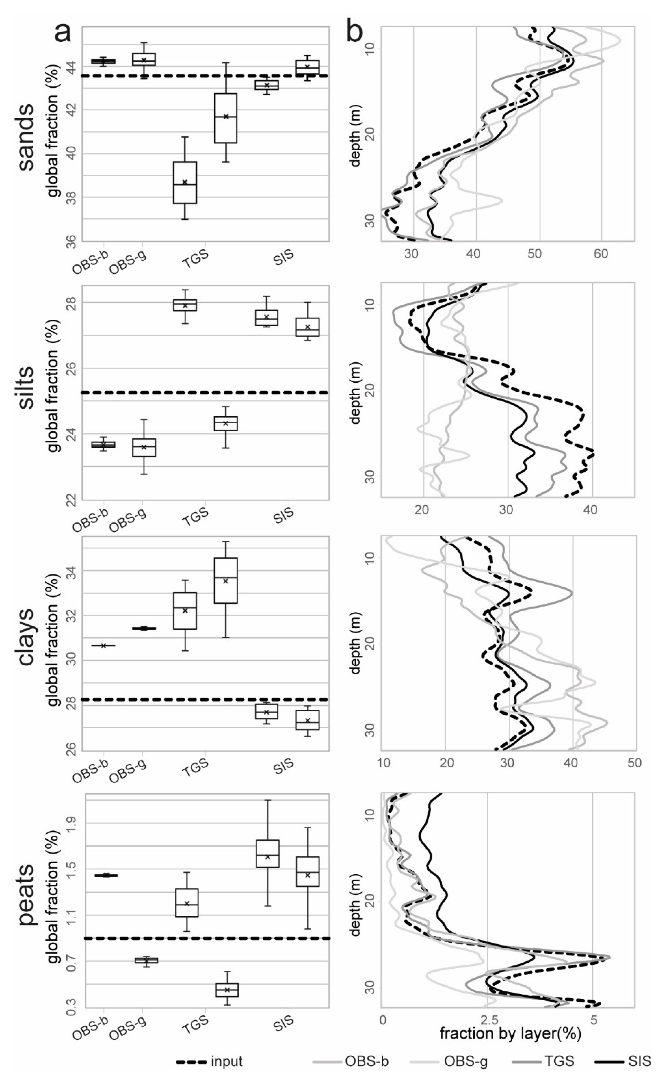
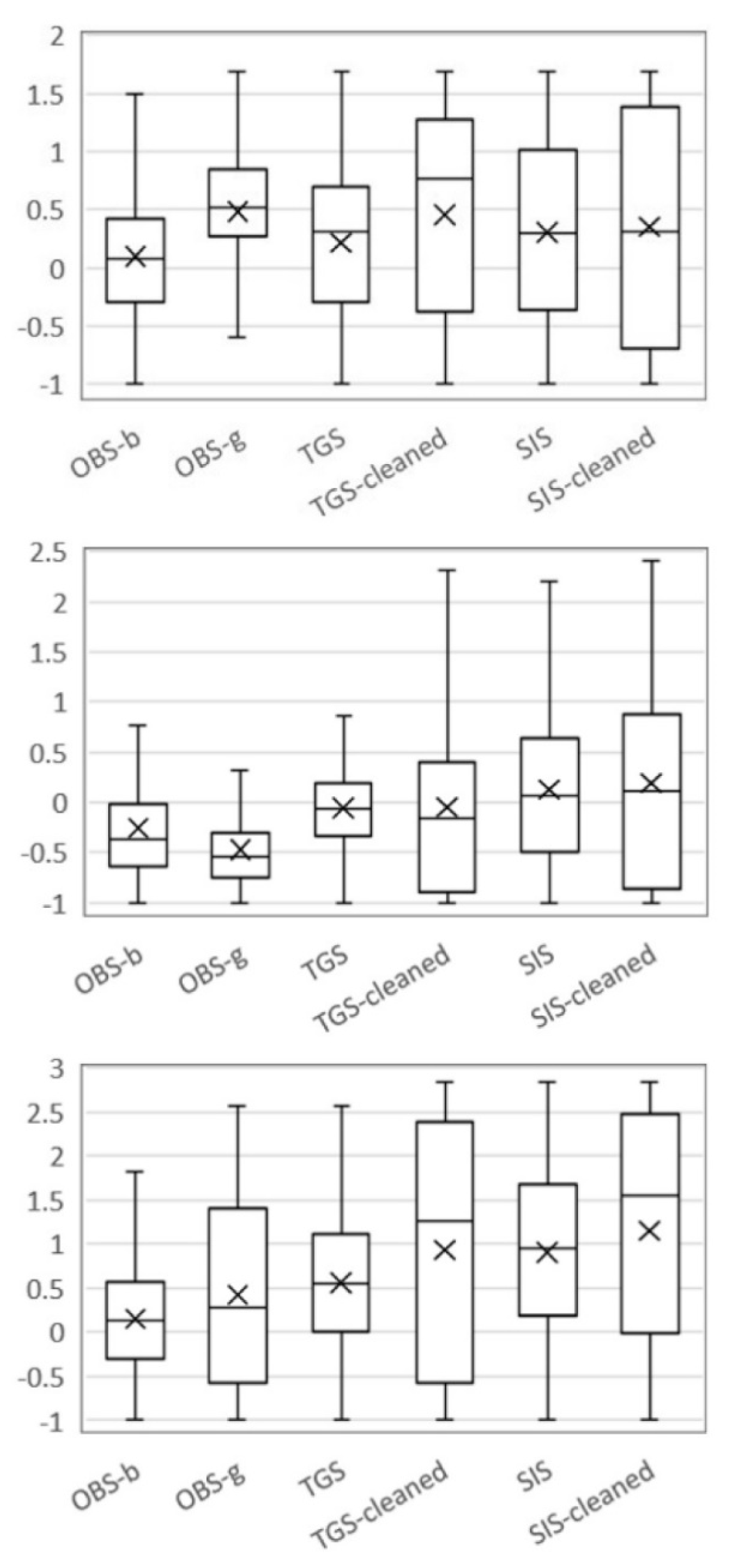
4.2. Conditioning to Input Data and Facies Prediction at Validation Boreholes

In modelling facies with OBS, changing the honoring priority setting had a relatively small effect on the actual conditioning to input data, with a maximum of ca. 55% of input cells honored by OBS-b as opposed to ca. 45% of OBS-g. After peats, which were nearly always honored by simulation, the sands (i.e., fluvial channel-fills) represent the best honored facies, followed by silts (i.e., levees associated to channels). In OBS-b, this is achieved by inserting channel and levee objects that show much less shape variability and are smaller and more numerous than those inserted by OBS-g (Table 4).
The shape size and variability of the objects inserted can be viewed to reflect the fact that when the honoring priority is assigned to borehole data, the algorithm will preferentially insert small objects because easier to fit to conditioning cells and facies proportions. Another observation is that, independently from the honoring priority settings, OBS models do not replicate satisfactorily either global facies fractions (e.g., up to ca. 4% departure from target fractions for silts) or vertical trends (Figure 7). As a result, there is generally a poor reproduction of input facies proportions. Conversely, because of the way pixel-based work, all realizations from SIS and TGS fully match facies from boreholes. However, input facies proportions were matched satisfactorily only by SIS realizations (departures <1% for all facies), whereas a systematic underestimation of sands (up to ca. 5%) in favor of silts and clays affects TGS realizations (Figure 7). Mildly cleaning TGS realizations from noise slightly improves simulated sand fractions, mostly at the expenses of silty and clays, while very little changes are to be seen after cleaning SIS realizations (right-hand box plots in Figure 7). Closeness of facies prediction ( C f r e l ) at cells crossed by validation boreholes (Figure 8) provides a mean for quantitatively ranking modelling results based on fairness of geostatistic estimation.
Since the validation cells for the facies peats where too few for a sound assessment, only the three most abundant facies are considered here. It is recalled that, following Equation (2), C f r e l values greater than 0 signifies that geostatistical prediction does better than simply predicting by abundance (and thus probability) of each facies in the input dataset. Therefore, in the box plots Figure 8 distributions of C f r e l with positive median indicate that the used modelling approach provided some prediction improvement in at least 50% of the cells where f has been encountered in a validation borehole and the greater the 25th percentile, the median, and the 75th percentile, the better the overall facies prediction. If sands are considered first, it can be noted how all the used modelling approaches (Figure 8a) yield some prediction improvement in at least of ca. 50% of the validation cells, with SIS providing by far the best results with a median of 0.3. Prediction is even better in the case of clays (Figure 8c), with SIS providing again the best results with a median of 0.9. Conversely, the ability to predict silts resulted to be much worse, with OBS and TGS populating validation cells with other facies in most of the cases (e.g., median is negative) and SIS returning a positive yet very small median value of C f r e l . Finally, one last observation regards the sensitivity of prediction to cleaning from noise pixel-based realization, which results in a weak to fair improvement for some of the facies (e.g., sands and clays in TGS and clays in SIS), counterbalanced by worsening for some others (e.g., silts in TGS and sands and silts in SIS). While in TGS these changes correlate with likewise changes of simulated facies fractions, which is explained by the fact that MAPS tends to disfavor the least abundant facies [21], in SIS no such correlation is seen, possibly because of the too subtle changes of simulated facies fractions after noise cleaning.

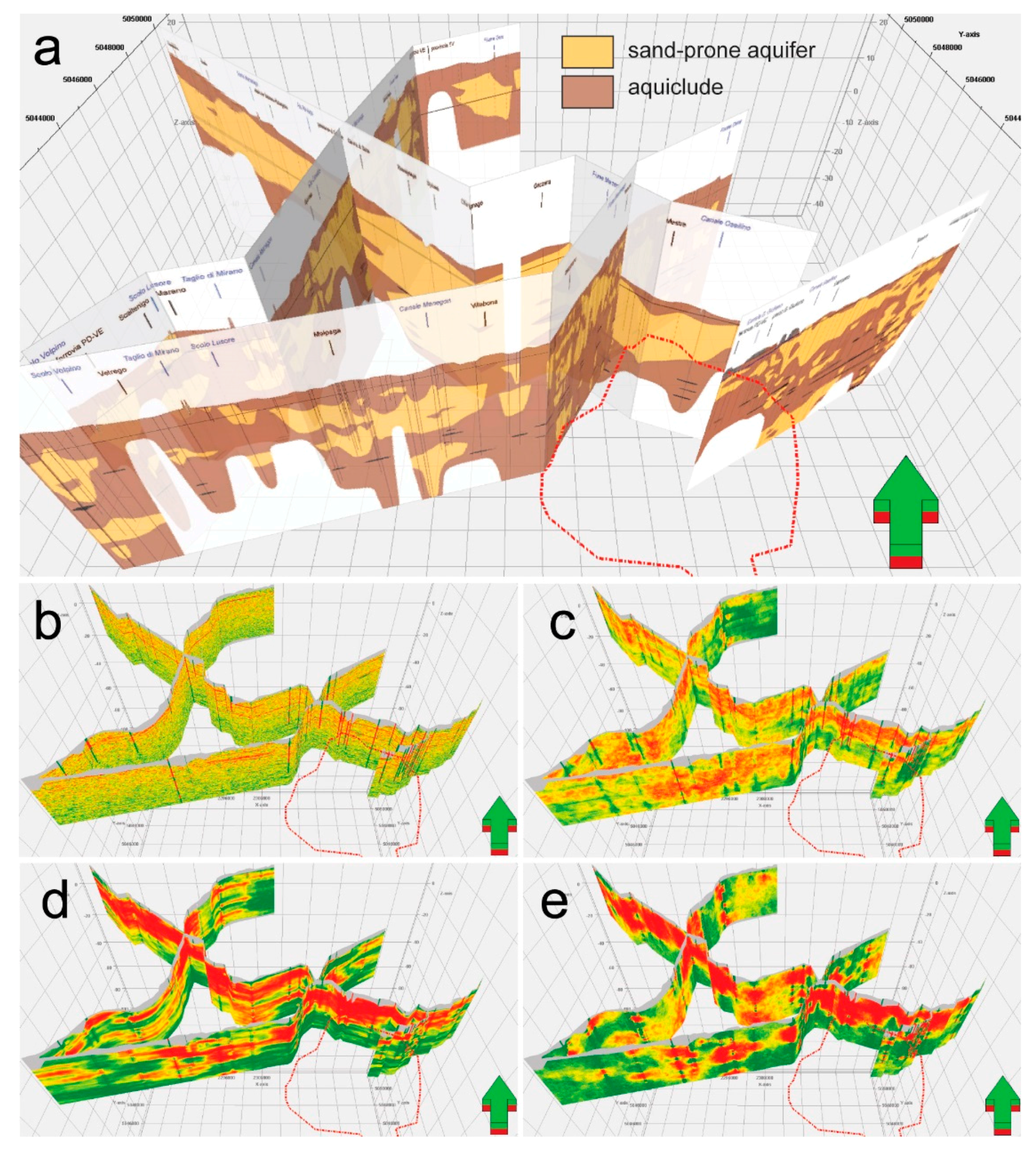
4.3. Sand Probability Models

Results from the alternative facies modelling approaches adopted in this study can be ranked based on ability to depict the extent and likely topology of highly conductive geobodies. This is done here focusing on sands only, since with a K of at least two orders of magnitude greater than other facies it might host most of the groundwater flow. In Figure 9, the boundary of the main aquifer sandbody in the shallow subsurface [27] is overlain onto alternative sand probability maps for comparison.
Disregarding the applied honoring priority, maps from OBS (Figure 9a,b) are typified by a relatively low overall probability, indicating a considerable uncertainty in locating sands. Yet, assigning the honoring priority to object geometry results at least in some clustering of high-range values parallel to axis and within the boundaries of the aquifer sandbody (Figure 9b). Although it can be speculated that a greater number of equiprobable realizations might have resulted in some improvement of sand probability models, most of the uncertainty associated to OBS facies models is viewed here to reflect the too low degree of borehole conditioning attained with the current simulation set up (see Section 4.2). Indeed, because different subsets of only about one half of the available input cells could be honored in each simulation run (see Section 4.2), OBS is left with too much degree of freedom for drawing facies at each cell, resulting in significant variability across different realizations. The better performance of the tested pixel-based algorithms (Figure 9c,e respectively) over OBS is suggested by most of the high-end values of the sand probability map from TGS and SIS clustering within the outline of the main sandbody. Also, it is noteworthy that noise cleaning reduces considerably the uncertainty in the sand probability model from TGS (Figure 9d), whereas it has very little impact on that from SIS (Figure 9f). Similar conclusions can be drawn from cross-sectional views (Figure 10 and Figure 11) which suggests OBS provides a fuzzy picture of sand distribution, whereas pixel-based algorithms were capable at replicating the topology of sandbodies proposed by [27], even in area with only a few conditioning boreholes (Figure 11b,c).
Yet, the TGS probability models depict a remarkably smoother and stratified subsurface structure than expected in a channelized alluvial fan such as BRM (Figure 11d,e).

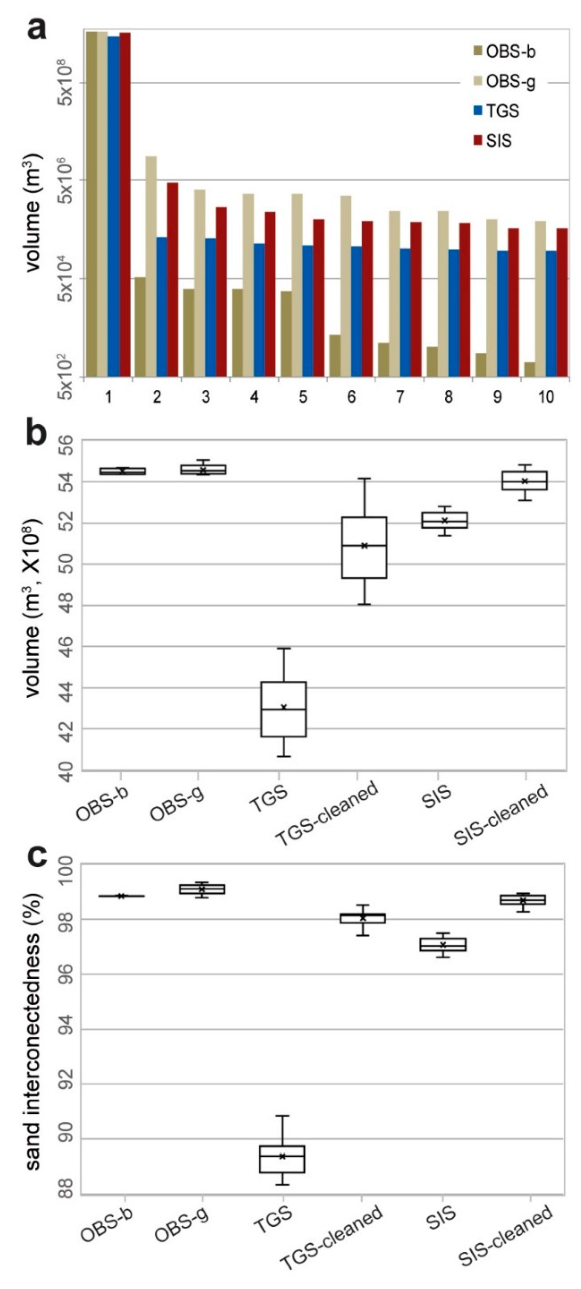
4.4. Connectivity of Modelled Sands

Calculation of connected sand volumes indicates that, irrespective of the algorithm used for facies simulation, there is one main sand geobody (the model aquifer, hereafter) with volumes in the range of 4.3–5.5 × 10⁹ m3, accompanied with several sandbodies smaller by four orders of magnitude (Figure 12a). Variability of this estimate is generally low across equiprobable realizations, reaching a maximum of 6% in the TGS realization set (Figure 12b), whereas it can be relatively large across alternative facies modelling approaches. In fact, TGS returns model aquifer volumes smaller (by at least 5.5 × 10⁸ m3) than obtained with SIS (Figure 12b), which is not surprising provided that the former algorithm systematically underestimates the sand fraction (see Section 4.1 and Section 4.2).
Since OBS was unsuccessful at honoring input data and the least successful in predicting facies, the connectivity structure resulting from using this method is considered here as highly unrealistic and thus not discussed further. On the other hand, statistics of model aquifer volumes from pixel-based facies models are interesting in that they illustrate how estimates obtained simulating hydrofacies might depend not only on fraction but also on degree of connectedness of simulated high-K facies. In fact, normalizing aquifer volumes by percent of total sand in each simulation highlights how the lower estimate of model aquifer volume from TGS relates to a noticeable difference of sand interconnectedness between TGS and SIS realizations (Figure 12c). Also, it can be seen how noise cleaning results in an increase of both model aquifer volumes and sand interconnectedness, especially when applied to TGS realizations.

4.5. Particle Tracking Results

Because of the poor results obtained with OBS, the particle tracking experiment was run on sample hydrofacies realizations from TGS and SIS only, before and after noise cleaning. Plotting particle injection vs. arrival layer at the four corners of the test volume (Figure 13) highlights how, especially before noise cleaning, the TGS example is typified by tracked arrivals that tend to be more evenly distributed vertically (i.e., by layer or depth) and correlated to layer of injection (left side of Figure 13a) compared to the SIS example (left side of Figure 13b), indicating a greater flow channeling in the latter.
Reiterating the experiment after noise cleaning (right-hand side of Figure 13a,b) results in turn in a more similar flow behavior across the two alternative facies models, though a greater flow anisotropy is still apparent in the SIS example. These results are interpreted here to reflect the highly disordered spatial variability of K resulting from widespread noise in raw TGS hydrofacies models, which ultimately translates into a more isotropic flow than expected in an alluvial aquifer with laterally extensive channel-fill sandbody. An appreciable anisotropy of the connectivity structure of the SIS model is also highlighted by time of particle arrivals which indicate preferential and faster flow along the N-S direction (Figure 14b), roughly parallel to local orientation of the BRM channel network. Even after cleaning hydrofacies realization from noise, time of particle arrivals indicate SIS and TGS models are associated with alternative connectivity structures (right side of Figure 14), suggesting that even at site with numerous conditioning boreholes the choice of algorithm might be critical to groundwater flow assessment.

5. Discussion

5.1. Which Modelling Algorithm Does Better with Lithology from Dense Borehole Data?

Results of this study confirm some of the well-known limitations of classical geostatistical algorithms in replicating the lithofacies heterogeneity of channelized alluvial sediments [1,2,11,12,13,14,37,38]. However, it was possible to rank the tested algorithms based on how closely they honored input data and predicted facies at validation boreholes [11], as well as they replicated the current hydrostratigraphic model of the study area [26]. Even though resulting in geologically realistic facies distributions, the Object-Based Simulation (OBS) of this study failed to achieve full conditioning to boreholes, as well as to reproduce global and layer-by-layer facies proportions. This reflects the unease of OBS at honoring dense input data by inserting user-defined objects and translated into much variability across equiprobable realizations and, ultimately, poor facies prediction. While it must be acknowledged that using a coarser grid layering (e.g., 0.5 m, corresponding to less than a half of the conditioning cells used here) might have allowed to fully honor input boreholes (albeit at the cost of less vertical detail), it must be concluded that OBS is not viable for capturing small-scale heterogeneity in densely investigated sites. By contrast, due to their fully conditional nature, facies models from the Truncated Gaussian Simulation (TGS) and the Sequential Indicator Simulation (SIS) do fully honor borehole data but fail to capture the curvilinear shapes typical of channelized alluvial sediments, thus resulting in a generally poor geological realism, especially of plan geometries. This has been widely documented in the literature and reflects the inadequateness of variogram ranges as a metric of spatial correlation of facies belonging to geobodies with complex 3D geometry [37]. However, SIS was able to better reproduce facies proportions and capture the WNW-ESE anisotropy of the BRM channel-network compared to TGS, as well as was less affected by presence of spurious cells assigned to outlier facies (i.e., noise). On the other hand, the widespread noise in TGS models is viewed here to reflect the implementation of a rule of lateral facies transition which, due to repeated fluvial channeling, is only rarely preserved in BRM and results therefore in erratic and presumably uncorrected facies estimation. Despite the poor geological realism of individual facies realizations, the sand probability models computed from TGS and SIS show a good match with the current knowledge of the BRM shallow aquifer. Similar conclusions can be drawn by closeness of facies prediction results, which suggests that the geostatistic estimate from the pixel-based methods does better than simply guessing facies based on their abundance in borehole cores. One concluding remark should address the borehole lithology data used in this study, which required to group the observed variety of soil types into a few operative facies of practical use for geostatistical modelling. Because detail and consistency of core descriptions were highly variable, and boreholes were too many to allow for a case-by-case sedimentological interpretation, no other criteria but dominant grain size could be used to define operative facies. As a result, the link between facies and component depositional elements of BRM can be strong (e.g., channel fills are in most cases represented by sands) but by no means exclusive (e.g., sands can occur in levees as well, whereas silts and clays can be locally intercalated within channel-fill sands), potentially undermining all those modelling approaches that rely on fixed facies transition rules and identity between facies and depositional objects, including OBS and TGS, as well as the nowadays highly popular Pluri-Gaussian [17] and the Multiple-Point Statistics [38]. It is therefore concluded that, especially when working with large borehole datasets where definition of operative facies can be weak, using SIS might still represent a pragmatic (it does not require any assumption on spatial relationship among facies) yet decent hydrofacies modelling choice.

5.2. Likely Implications for Aquifer and Groundwater Flow Assessment

Given the complexity of the groundwater flow in study site [27,28,29,30], a validation of hydrofacies models against direct hydrogeological observations was not undertaken in this work. Nonetheless, in Section 4.3 it has been shown that both TGS and SIS were able to replicate with good confidence the current hydrostratigraphic model of BRM [27], suggesting these methods can be used in similar contexts for expeditious appraisal of aquifer depth even at sites with boreholes spacing in order of a few to several hundred meters. In addition, in Section 4.4 and Section 4.5, it is shown that hydrofacies models from TGS and SIS are associated with different degree of sand connectedness and simulated flow behavior chiefly due to widespread noise in TGS simulation results. Such noise has in fact a twofold impact on connectivity in that it can both act as a ‘thief’ to the model aquifer volumes, for example when a consistent fraction of simulated sand occurs as isolated cells in a low-K background, and considerably increase flow path tortuosity, for example when the model aquifer is speckled with numerous cells populated with low-K facies. The latter aspect is particularly well expressed by particle tracking results of Section 4.5, where the widespread noise in the TGS hydrofacies realization translates into a spatially disordered distribution of K and, ultimately, into a very diffuse flow (i.e., there is low variability in the number of particles reaching both the different layers and corners of the test volume) strikingly contrasting with presence in BRM of high-K channel-fill sandbodies. Although it has been shown that noise cleaning may dampen differences between alternative hydrofacies models, it is advised that the admissible degree of noise cleaning should be judged based on a sound estimation of hydrofacies abundance proportions, so as to avoid aquifer volume and connectedness misestimations.

6. Conclusions

Three geostatistical algorithms commonly employed for sedimentary facies and hydrofacies modelling, namely the Object-Based Simulation (OBS), the Sequential Indicator Simulation (SIS), and the Truncated Gaussian Simulation (TGS), were tested using a large borehole lithology dataset from the channelized alluvial deposits of the Brenta River Megafan (BRM, Upper Pleistocene), NE Italy. The specific objective was to explore algorithm strengths and weaknesses, with special reference to hydrogeological applications at sites with dense borehole information. Key findings are as follows:
  • Though compromising with geological realism of facies clusters shapes, TGS and SIS are better suited in place of OBS for their ease of conditioning to closely spaced boreholes.
  • Pixel-based facies models of this study, especially those from TGS, suffer for ‘noise’ in form of unwanted isolated cells taking outlier hydrofacies values, which require cleaning for better assessment of aquifer facies distribution.
  • SIS provides better facies prediction and renders a less noisy picture of subsurface geology than TGS, without requiring assumptions about spatial relationship among operative facies, which makes it the best suited for use with large borehole lithology datasets lacking detail and quality consistency.
  • Statistics of connected sands and results of the particle tracking simulation indicate TGS and SIS hydrofacies models are associated with significantly different aquifer connectivity scenarios, e.g., a relatively poorly connected aquifer (TGS) typified by diffuse, nearly isotropic flow as opposed to a better-connected aquifer (SIS) featuring preferential flow paths hosted within the sandy channel-fills of BRM.
  • Differences between the two alternative pixel-based aquifer models are due to widespread noise in TGS realizations, suggesting that noise cleaning should be considered and implemented with care before simulating groundwater flow.

Author Contributions

Conceptualization, M.M., F.F., G.P.B.; Methodology, M.M and J.T..; Software, M.M. and J.T.; Validation, G.P.B., Y.Y. and Z.Z.; Formal Analysis, M.M. and J.T.; Investigation, M.M. and J.T.; Resources, M.M., F.F., G.P.B and J.T.; Data Curation, M.M., G.P.B. and J.T.; Writing-Original Draft Preparation, M.M.; Writing-Review & Editing, M.M., F.F., G.P.B.; Visualization, M.M. and J.T.; Supervision, M.M., F.F., G.P.B.; Project Administration, M.M.

Funding

This research received no external funding.

Acknowledgments

The two anonymous reviewers are thanked for their useful comments. Provincia di Venezia is warmly acknowledged for providing the dataset used to make this study, along with additional GIS, cartographic, and bibliographic material. We are also grateful to Schlumberger™ which has supplied an academic license of Petrel 2014™ to the University of Milan.

Conflicts of Interest

The authors declare no conflict of interest.

References

  1. Dell’arciprete, D.; Felletti, F.; Bersezio, R. Simulation of fine-scale heterogeneity of meandering river aquifer analogues: Comparing different approaches. In geoENV VII—Geostatistics for Environmental Applications, Quantitative Geology and Geostatistics; Atkinson, P., Lloyd, C., Eds.; Springer: Dordrecht, The Netherlands, 2010; Volume 16, pp. 127–137. [Google Scholar] [CrossRef]
  2. Dell’arciprete, D.; Bersezio, R.; Felletti, F.; Giudici, M.; Comunian, A.; Renard, P. Comparison of three geostatistical methods for hydrofacies simulation: A test on alluvial sediments. Hydrogeol. J. 2012, 20, 299–311. [Google Scholar] [CrossRef]
  3. Colombera, L.; Felletti, F.; Mountney, N.P.; McCaffrey, W.D. A database approach for constraining stochastic simulations of the sedimentary heterogeneity of fluvial reservoirs. Am. Assoc. Pet. Geol. Bull. 2012, 96, 2143–2166. [Google Scholar] [CrossRef]
  4. Colombera, L.; Mountney, N.P.; Felletti, F.; McCaffrey, W.D. Models for guiding and ranking well-to-well correlations of channel bodies in fluvial reservoirs. Am. Assoc. Pet. Geol. Bull. 2014, 98, 1943–1965. [Google Scholar] [CrossRef] [Green Version]
  5. Comunian, A.; De Micheli, L.; Lazzati, C.; Felletti, F.; Giacobbo, F.; Giudici, M.; Bersezio, R. Hierarchical simulation of aquifer heterogeneity: Implications of different simulation settings on solute-transport modelling. Hydrogeol. J. 2016, 24, 319–334. [Google Scholar] [CrossRef]
  6. Fogg, G.E.; Noyes, C.D.; Carle, S.F. Geologically based model of heterogeneous hydraulic conductivity in an alluvial setting. Hydrogeol. J. 1998, 6, 131–143. [Google Scholar] [CrossRef]
  7. Anderson, M.P.; Aiken, J.S.; Webb, E.K.; Mickelson, D.M. Sedimentology and hydrogeology of two braided stream deposits. Sediment. Geol. 1999, 129, 187–199. [Google Scholar] [CrossRef]
  8. De Marsily, G.; Delay, F.; Gonçalvès, J.; Renard, P.; Teles, V.; Violette, S. Dealing with spatial heterogeneity. Hydrogeol. J. 2005, 13, 161–183. [Google Scholar] [CrossRef] [Green Version]
  9. Bianchi, M.; Zheng, C. A lithofacies approach for modelling non-Fickian solute transport in a heterogeneous alluvial aquifer. Water Resour. Res. 2016, 52, 552–565. [Google Scholar] [CrossRef]
  10. Matheron, G. Random Functions and their Application in Geology. In Geostatistics Computer Applications in the Earth Sciences; Merriam, D.F., Ed.; Springer: Boston, MA, USA, 1970; pp. 79–87. [Google Scholar]
  11. Pyrcz, M.J.; Deutsch, C.V. Geostatistical Reservoir Modelling, 2nd ed.; Oxford University Press: Oxford, UK, 2014; p. 348. ISBN 9780199731442. [Google Scholar]
  12. Seifert, D.; Jensen, J.L. Object and pixel-based reservoir modelling of a braided fluvial reservoir. Math. Geol. 2000, 32, 581–603. [Google Scholar] [CrossRef]
  13. Deutsch, C.V.; Tran, T.T. FLUVSIM: A program for object-based stochastic modelling of fluvial depositional systems. Comput. Geosci. 2002, 28, 525–535. [Google Scholar] [CrossRef]
  14. Keogh, K.J.; Martinius, A.W.; Osland, R. The development of fluvial stochastic modelling in the Norwegian oil industry: A historical review, subsurface implementation and future directions. Sediment. Geol. 2007, 202, 249–268. [Google Scholar] [CrossRef]
  15. Pyrcz, M.J.; Boisvert, J.B.; Deutsch, C.V. A library of training images for fluvial and deepwater reservoirs and associated code. Comput. Geosci. 2008, 34, 542–560. [Google Scholar] [CrossRef]
  16. Deutsch, C.V.; Journel, A.G. GSLIB: Geostatistical Software Library and User's Guide, 2nd ed.; Oxford University Press: New York, NY, USA, 1998; p. 369. [Google Scholar]
  17. Beucher, H.; Renard, D. Truncated Gaussian and derived methods. C. R. Geosci. 2016, 348, 510–519. [Google Scholar] [CrossRef]
  18. Dethlefsen, F.; Ebert, M.; Dahmke, A. A geological database for parameterization in numerical modelling of subsurface storage in northern Germany. Environ. Earth Sci. 2014, 71, 2227–2244. [Google Scholar] [CrossRef]
  19. Vázquez-Suñé, E.; Marazuela, M.Á.; Velasco, V.; Diviu, M.; Pérez-Estaún, A.; Álvarez-Marrón, J. A geological model for the management of subsurface data in the urban environment of Barcelona and surrounding area. Solid Earth 2017, 7, 1317. [Google Scholar] [CrossRef]
  20. Pham, H.V.; Tsai, F.T.C. Modelling complex aquifer systems: A case study in Baton Rouge, Louisiana (USA). Hydrogeol. J. 2017, 25, 601–615. [Google Scholar] [CrossRef]
  21. Deutsch, C.V. Cleaning categorical variable (lithofacies) realizations with maximum a-posteriori selection. Comput. Geosci. 1998, 24, 551–562. [Google Scholar] [CrossRef]
  22. Hong, S.; Deutsch, C.V. Another Look at Realization Cleaning; Centre for Computational Geostatistics Report 12; University of Alberta: Edmonton, AB, Canada, 2010; p. 118. [Google Scholar]
  23. Vitturi, A.; Bondesan, A.; Fontana, A.; Mozzi, P.; Primon, S.; Bassan, V. Geologia. In Atlante Geologico Della Provincia di Venezia—Note Illustrative, Quarto d’Altino (Venezia); Vitturi, A., Bassan, V., Mazzuccato, A., Primon, S., Bondesan, A., Ronchese, F., Zangheri, P., Eds.; Arti Grafiche Venete: Venezia, Italia, 2011; pp. 333–357. ISBN 9788890720703. [Google Scholar]
  24. Bondesan, A.; Primon, S.; Bassan, V.; Vitturi, A. (Eds.) Le Unità Geologiche Della Provincia di Venezia; Provincia di Venezia, Servizio Geologico e Difesa del Suolo: Venezia, Italia, 2008. [Google Scholar]
  25. Fontana, A.; Mozzi, P.; Marchetti, M. Alluvial fans and megafans along the southern side of the Alps. Sediment. Geol. 2014, 301, 150–171. [Google Scholar] [CrossRef]
  26. Donnici, S.; Serandrei-Barbero, R.; Bini, C.; Bonardi, M.; Lezziero, A. The caranto paleosol and its role in the early urbanization of Venice. Geoarchaeology 2011, 26, 514–543. [Google Scholar] [CrossRef]
  27. Fabri, P.; Zàngheri, P.; Bassan, V.; Fagarazzi, E.; Mazzuccato, A.; Primon, S.; Zogno, C. Sistemi Idrogeologici Della Provincia di Venezia: Acquiferi Superficiali; Provincia di Venezia, Servizio Geologico, Difesa del Suolo e Tutela del Territorio: Venezia, Italia, 2013. [Google Scholar]
  28. Carbognin, L.; Rizzetto, F.; Tosi, L.; Teatini, P.; Gasparetto-Stori, G. The salt intrusion in the Venetian lagoon area: II. The southern basin. Geol. Appl. 2005, 2, 124–229. [Google Scholar]
  29. Da Lio, C.; Tosi, L.; Zambon, G.; Vianello, A.; Baldin, G.; Lorenzetti, G.; Manfè, G.; Teatini, P. Long-term groundwater dynamics in the coastal confined aquifers of Venice (Italy). Estuar. Coast. Shelf Sci. 2013, 135, 248–259. [Google Scholar] [CrossRef]
  30. Beretta, G.P.; Terrenghi, J. Groundwater flow in the Venice lagoon and remediation of the Porto Marghera industrial area (Italy). Hydrogeol. J. 2017, 25, 847–861. [Google Scholar] [CrossRef]
  31. Associazione Geotecnica Italiana. Raccomandazioni Sulla Programmazione ed Esecuzione Delle Indagini Geotecniche; AGI; SGE: Padova, Italy, 1977. [Google Scholar]
  32. Folk, R.L. Petrology of Sedimentary Rocks; Hemphill Publishing Company: Austin, TX, USA, 1980. [Google Scholar]
  33. Daly, C.; Quental, S.; Novak, D. A faster, more accurate Gaussian simulation. In Proceedings of the GeoCanada Conference, Calgary, AB, Canada, 10–14 May 2010. [Google Scholar]
  34. Deutsch, C.V. A Short Note on Cross Validation of Facies Simulation Methods; Centre for Computational Geostatistics Annual Report, Report 1; University of Alberta: Edmonton, AB, Canada, 1998; p. 109. [Google Scholar]
  35. Harbaugh, A.W. MODFLOW-2005, the US Geological Survey Modular Ground-Water Model: The Ground-Water Flow Process; Department of the Interior, US Geological Survey: Reston, VA, USA, 2005.
  36. Pollock, D.W. Semianalytical Computation of Path Lines for Finite-Difference Models. Groundwater 1998, 26, 743–750. [Google Scholar] [CrossRef]
  37. Pollock, D.W. User Guide for MODPATH Version 6—A Particle-Tracking Model for MODFLOW. US Geological Survey Techniques and Methods 6-A41; Department of the Interior, US Geological Survey: Reston, VA, USA, 2012.
  38. Jha, S.K.; Mariethoz, G.; Mathews, G.; Vial, J.; Kelly, B.F. Influence of Alluvial Morphology on Upscaled Hydraulic Conductivity. Groundwater 2016, 54, 384–393. [Google Scholar] [CrossRef] [PubMed]
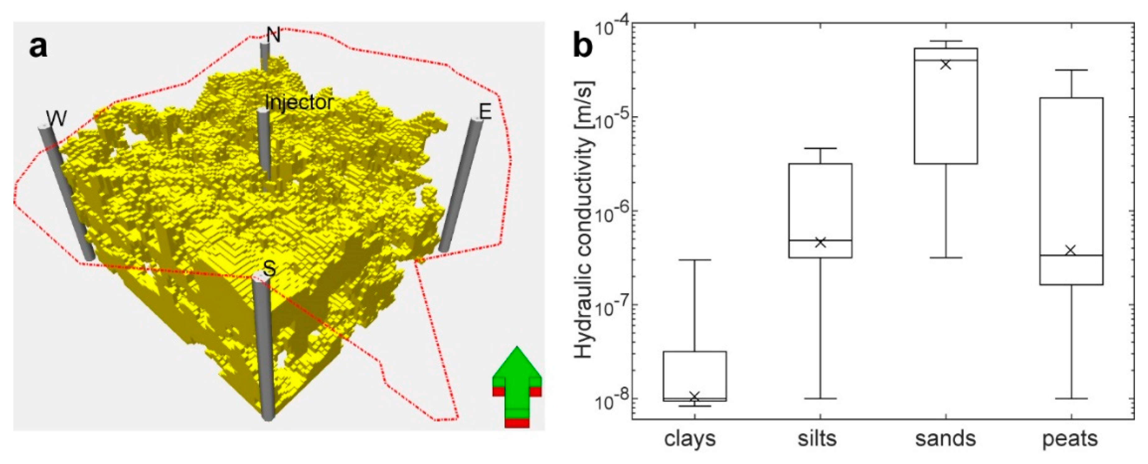
Figure 1. (a) Simplified geomorphological sketch of the Friulan-Venetian Plain outlining the main alluvial fans of late Quaternary age (modified, from [25]). Legend: (1) Brenta; (2) Montebelluna; (3) Piave, and (4) Adige; (b) Detail of the study area with outline of the ‘Petrolchimico’ and location of boreholes used for geostatistical modelling and validation.
Water 10 00844 g001
Figure 2. West-looking view of the model domain with top and bottom bounding stratigraphic surfaces and the available boreholes penetrating the Late Glacial Maximum deposits of the Brenta.
Water 10 00844 g002
Figure 3. (a) Likely plan-view topology of the aquifer sandbodies in the shallow subsurface of the study area (modified, after [27]); (b) Geological cross-section illustrating the lithofacies heterogeneity of the Late Pleistocene alluvial deposits addressed in this study (modified, after [24]).
Water 10 00844 g003
Figure 4. Breakdown of operative facies by component soil types named after the sedimentary clastic rock classification of [32].
Water 10 00844 g004
Figure 5. (a) Experimental set up of the particle tracking simulation with location of the injector and the receiving wells; (b) Box plots (logarithmic scale) of hydraulic conductivity K measurements from [26] by operative facies. Box boundaries indicate 25th percentile and 75th percentile, whiskers indicate maximum and minimum values, whereas the line and the cross within the box indicate the median and the mean values, respectively.
Water 10 00844 g005
Figure 6. Fence diagrams (left) and representative cross-sections (right) through sample facies realizations obtained with (a,b) the Object Based Simulation assigning honoring priority to either borehole data or object geometry; (c,d) the Truncated Gaussian Simulation prior and after noise cleaning, respectively; and (e,f) the Sequential Indicator Simulation prior and after noise cleaning. Vertical exaggeration is 200×.
Water 10 00844 g006aWater 10 00844 g006b
Figure 7. (a) Box plots showing the variability of simulated facies fractions from the Object-based Simulation with honoring priority assigned to either borehole data (OBS-b) or object geometry (OBS-g), the Truncated Gaussian Simulation (TGS) and the Sequential Indicator Simulation (SIS). For TGS and SIS, fractions before and after noise cleaning are plotted for comparison; (b) Vertical proportion curves of simulated facies from sample realizations. In both graph sets, the bold dashed line indicates facies fractions from input borehole data.
Water 10 00844 g007
Figure 8. Box plots of values of closeness of prediction of sands (top), silts (middle), and clays (bottom) from the alternative facies simulation approaches adopted in this study. For SIS and TGS, values calculated after noise cleaning are reported for comparison.
Water 10 00844 g008
Figure 9. Sand probability maps at a depth of 10 m below ground level calculated from the Object-Based Simulation with honoring priority assigned to (a) borehole data and (b) object geometry, the Truncated Gaussian Simulation prior (c) and after (d) noise cleaning, and the Sequential Indicator Simulation prior (e) and after (f) noise cleaning. The dashed lines are the boundaries of the main aquifer sandbody from [27].
Water 10 00844 g009
Figure 10. Cross-section (see Figure 3 for location and comparison with the geological cross-section after [24]) through sand probability models calculated from the Object-Based Simulation with honoring priority assigned to (a) borehole data and (b) object geometry, the Truncated Gaussian Simulation prior (c) and after (d) noise cleaning, and the Sequential Indicator Simulation prior (e) and after (f) noise cleaning.
Water 10 00844 g010
Figure 11. Fence diagrams (see Figure 3a for location) through (a) the hydrostratigraphic model from [27] and sand probability models from the Object-Based Simulation with honoring priority assigned to either (b) borehole data or (c) object geometry, and (d) the Truncated Gaussian Simulation and (e) the Sequential Indicator Simulation after noise cleaning.
Water 10 00844 g011
Figure 12. (a) Bar chart of volumes (logarithmic scale, base = 100) of the ten largest geobodies comprised of connected sands from the Object-based Simulation with honoring priority assigned to either borehole data (OBS-b) or object geometry (OBS-g), the Truncated Gaussian Simulation (TGS), and the Sequential Indicator Simulation (SIS); Box plots of (b) volumes of the largest geobody of connected sands (i.e., the model aquifer) and (c) ratio of model aquifer volume to total sand volume (i.e., sand interconnectedness, see text for explanation) calculated from the full sets of facies realization.
Water 10 00844 g012
Figure 13. Scatter plots of injection vs. arrival layer at the four cardinal corners (N, E, S, and W, clockwise from top left of each pane; see Figure 5a) of the test volume from the particle tracking experiment run on sample facies realization from (a) the Truncated Gaussian Simulation and (b) the Sequential Indicator Simulation prior (left) and after (right) noise cleaning. The background color (see legend at the bottom left) indicates the cumulative number of arrivals averaged over five layers. R2 is the Pearson correlation coefficient for linear regression fits passing through the origin.
Water 10 00844 g013
Figure 14. Number vs. time of arrival of tracked particles at the four cardinal corners of the facies models obtained using (a) the Truncated Gaussian Simulation and the (b) Sequential Indicator Simulation, prior to (left) and after noise cleaning (right).
Water 10 00844 g014
Table 1. Dominant depositional process and environment, abundance in the borehole dataset (as percent of cumulative thickness), and hydraulic conductivity (K) of the operative facies used in geostatistical modelling. The facies ordering in the table reflects the transition rule adopted in modelling facies with the Truncated Gaussian Simulation.
FaciesDepositional EnvironmentDepositional ProcessAbundance (%)Mean K (m/s)
sandsfluvial channelpoint bar migration43.22.00 × 10−5
siltsleveeoverbanking27.55.00 × 10−7
claysfloodplainoverbanking28.41.00 × 10−8
peatspeatlandplant debris accumulation 0.93.50 × 10−7
Table 2. Order of insertion, component facies, and numerical descriptors of shape, size, and layout of the depositional object used in the Object-Based Simulation.
Object TypeFaciesInsertion Order/Replacement RulesShape Size, Layout and Orientation
Cross-SectionalPlan-View MinMeanMaxDrift 1
(m)(%)
fluvial channelsandsafter peats; can replace peatshalf-pipestring-like, sinuous width-300-1
lengthinfinite
thickness12.550.3
orientation (°)-110-0.1
sinuosity amplitude-500-0.3
wave-length-2500-0.5
leveesiltsin tandem with/on both sides of channels; can replace peatswedgestring-like, sinuous width0.63 × channel width0.5
lengthinfinite
thickness0.63 × channel thick.0.5
orientation/sinuositysame as channels
backgroundclayslast, fills in gaps between previously inserted objectsn/a
peat accumulationpeatsfirst to be insertedelliptical ellipticalwidth1002502000-
length1006255000-
thickness0.20.51-
orientation (°)-110-0.1
Note: 1 Drift is a multiplier expressing the tolerance allowed to the algorithm to adapt sizes of inserted objects to conditioning borehole data.
Table 3. Parameters of the theoretical variograms used as input for the Sequential Indicator Simulation and the Truncated Gaussian Simulation (last row). Information reported in brackets refer to the second structure (if any) used for fitting the experimental variogram.
Operative FaciesMajor Direction (°)Function Type 1SillRanges (m)
MajorMinorVertical
sands105exp (exp)0.7 (0.3)215 (4500)210 (1500) 3.7 (16.4)
silts180exp (exp)0.7 (0.3)70 (3100)35 (3000)2.6 (17.8)
clays110exp (exp)0.7 (0.3)50 (3100)50 (1300)2.7 (25)
peatsn/aexp1.05005001.1
continuous variable 2110exp (sph)0.6 (0.4)90 (10,700)30 (10500)1.3 (9.5)
Note: 1 exp and sph are abbreviations for exponential and spherical model functions used for fitting the experimental variogram; 2 normal-score continuous variable into which operative facies are converted in TGS.
Table 4. Report of modelling parameters by object type, including fraction of conditioning cells honored in the simulation, of two sample facies realizations of BRM from the Object-based Simulation with honoring priority assigned to either borehole data (OBS-b) or object geometry (OBS-g). Values in brackets are standard deviations.
Object Type OBS-bOBS-g
fluvial channels honored cells (%)5045
number of inserted items25251002
width125 (5)300 (0)
thickness1.15 (0.3)2.83 (0.81)
leveeshonored cells (%)3533
number of inserted items25251002
width75 (3.23)189 (0)
thickness0.72 (0.04)1.15 (0)
peatshonored cells (%)10099
number of inserted items957931
maximum length967 (401)906 (423)
minimum length645 (399) 608 (411)

