Numerical Simulation of the Interaction between Phosphorus and Sediment Based on the Modified Langmuir Equation

Abstract

Phosphorus is the primary factor that limits eutrophication of surface waters in aquatic environments. Sediment particles have a strong affinity to phosphorus due to the high specific surface areas and surface active sites. In this paper, a numerical model containing hydrodynamics, sediment, and phosphorus module based on improved Langmuir equation is established, where the processes of adsorption and desorption are considered. Through the statistical analysis of the physical experiment data, the fitting formulas of two important parameters in the Langmuir equation are obtained, which are the adsorption coefficient, $k_a$, and the ratio k between the adsorption coefficient and the desorption coefficient. In order to simulate the experimental flume and get a constant and uniform water flow, a periodical numerical flume is built by adding a streamwise body force, F_x. The adsorbed phosphorus by sediment and the dissolved phosphorus in the water are separately added into the Advection Diffusion equation as a source term to simulate the interaction between them. The result of the numerical model turns out to be well matched with that of the physical experiment and can thus provide the basis for further analysis. With the application of the numerical model to some new and relative cases, the conclusion will be drawn through an afterwards analysis. The concentration of dissolved phosphorus proves to be unevenly distributed along the depth and the maximum value approximately appears in the 3/4 water depth because both the high velocity in the top layer and the high turbulence intensity in the bottom layer can promote sediment adsorption on phosphorus.

1. Introduction

Phosphorus (P) is one of the main limiting factors for eutrophication in most lakes and rivers [1]. Therefore, the migration and transformation processes of phosphorus play an important role in aquatic environments [2]. Sediment particles have a strong affinity to phosphorus due to the high specific surface areas and surface active sites [3]. Phosphorus absorbed by the sediment accumulates in the riverbed as sediment settles [4] and may be released by resuspension [5].

The main interactions between sediment and phosphorus are adsorption and desorption [6]. There are many factors affecting these interactions such as the physical [7] and chemical [8] properties of sediment, the water environment chemical properties [9], the adsorbate and sorbent concentration, and the hydrodynamic characteristics. Usually, the amount of adsorption per unit mass of sediment in the quasi-equilibrium state increases as the initial phosphorus concentration in water increases or as the sediment concentration decreases [10]. The increase of velocity can greatly affect the adsorption and desorption due to flow turbulence [11].

Besides the physical experiments, a great number of water quality models have been developed over recent decades [12]. Early models often ignored the effect of sediment on phosphorus transport [13]. Subsequently, lots of models considering the influence of sediment were proposed [14]. Most of these models considered that with empirical parameters such as a linear distribution coefficient $k_d$ of adsorption thermodynamics [15], or adsorption rate $k_1$ and desorption rate $k_2$ of adsorption kinetics [16]. Other simplifications included a sedimentation coefficient and a suspension coefficient, or a constant phosphorus release rate at the sediment-water surface [14]. It is very difficult to determine these parameters reasonably for lacking fundamental mechanistic analysis, and they are site-specific and not easily extended.

This paper develops a model regarding hydrodynamics and the interactions of suspended sediment and phosphorus based on the Langmuir equation. Sediment samples are collected from the Wujiadu gauging station of the main stream in Huaihe River. After finishing the dynamic water physical experiments, the adsorption coefficient in the Langmuir adsorption kinetic model, $k_a$, and the ratio k between $k_a$ and the desorption coefficient $k_b$ are obtained. By separately fitting these values, two formulas are deduced. One is the relationship between k and suspended sediment S, cross-sectional average velocity v, initial phosphorus concentration ${\mathrm{C}}_0$. The other is the relationship between $k_a$ and v, ${\mathrm{C}}_0$. Then k and $k_a$ are applied to the Langmuir equation in the numerical model for verification and application. The purpose of this study is to get the distribution between adsorbed phosphorus on the suspended sediment and dissolved phosphorus in the water, and find out how hydrodynamic condition affects the phosphorus transport.

2. Materials and Methods

2.1. Sediment Collection and Dynamic Water Experiments

Sediment samples were collected from a depth of >5 cm from the bank of Huaihe River at the Wujiadu gauging station in October 2013. In order to get uniformly distributed particle sized and clean sediment, all points were far away from scoured riverbeds and pollutant discharge ports. Sediments were immersed in deionized water for a month and then were air-dried in a ventilated environment. After being screened through 200 mesh sieves, particles finer than 90 μm were analyzed in the physical experiment. The median diameter of the samples was 22.7 μm, and the other two typical particle size in the sediment distribution curve $D_{10}$ and $D_{90}$ were 3.3 μm and 60 μm, respectively.

The dynamic water experiment was carried out in an elongated annular flume, which did not break up the sediment flocs when the flow is propelled by a Plexiglas gear instead of a water pump. A defined amount of sediment and $\mathrm{K}{\mathrm{H}}_2\mathrm{P}{\mathrm{O}}_4$ solution of known concentration was added to the water at the beginning of the experiment, as shown in

Table 1. C₀, S, v and the balanced adsorbed phosphorus amount per unit mass sediment Ne of various cases in the physical experiments.

Case	C0 (mg/L)	S (g/L)	v (m/s)	Ne (mg/g)
1	0.5	1	0.515	0.0614
2	0.5	1	0.48	0.062
3	0.5	1	0.44	0.0662
4	1	1	0.515	0.072
5	1	1	0.48	0.0787
6	1	1	0.44	0.0817
7	3	0.5	0.515	0.1431
8	3	0.5	0.48	0.1289
9	3	0.5	0.44	0.1084
10	3	0.5	0.39	0.1017
11	3	1	0.515	0.112
12	3	1	0.48	0.102
13	3	1	0.44	0.0885
14	3	1	0.39	0.0587
15	3	1.5	0.515	0.0907
16	3	1.5	0.48	0.0783
17	3	1.5	0.44	0.065
18	3	1.5	0.39	0.041
19	3	2	0.515	0.0702
20	3	2	0.48	0.0629
21	3	2	0.44	0.054
22	3	2	0.39	0.0332
23	5	1	0.515	0.1272
24	5	1	0.48	0.1102
25	5	1	0.44	0.1052

. The rotational speed was set at a certain value and was kept running for 24 h. Samples were filtered through a 0.45 μm filter membrane and non-absorbed phosphorus was determined using a molybdenum blue method on ultraviolet-visible spectrophotometer (TU-1810PC, Persee Co., Beijing, China). The amount of adsorbed phosphorus per unit mass sediment, Ne, at an equilibrium state of different cases were also shown in Table 1. During the experiments, the indoor temperature and the water pH were 21 ± 2 °C and 6.5–7.0, respectively. The detailed description of the physical experiment can be found in the literature [10].

2.2. Adsorption Parameters

There are two kinds of classical adsorption theories. One is adsorption isotherm model for studying the phosphorus distribution during the equilibrium, such as Langmuir model and Freundlich model [17]. Another is adsorption kinetic model for studying the dynamic phosphorus distribution with time increasing, such as Elovich equation [18], parabolic equation [6] and Langmuir model. According to the theory proposed by Huang S.L. in 1997 [19], the adsorbed phosphorus amount per unit mass by sediment at an equilibrium state relates to ${\mathrm{C}}_0$, S, maximum amount of adsorption ${\mathrm{B}}_{\mathrm{m}}$ and k. Among them, ${\mathrm{B}}_{\mathrm{m}}$ is only related to the characteristic of specific sediment. In this paper, ${\mathrm{B}}_{\mathrm{m}}$ is given 0.15 mg/g according to the batch reactor experiments [10]. Thus we can predicate the adsorbed phosphorus amount per unit mass by sediment if k is given. And another parameter $k_a$ represents the speed of the reaction.

2.2.1. The Ratio k between $k_a$ and $k_b$

In this paper, the formula of k is given by the fitting method according to the results of the physical experiments of our research group.

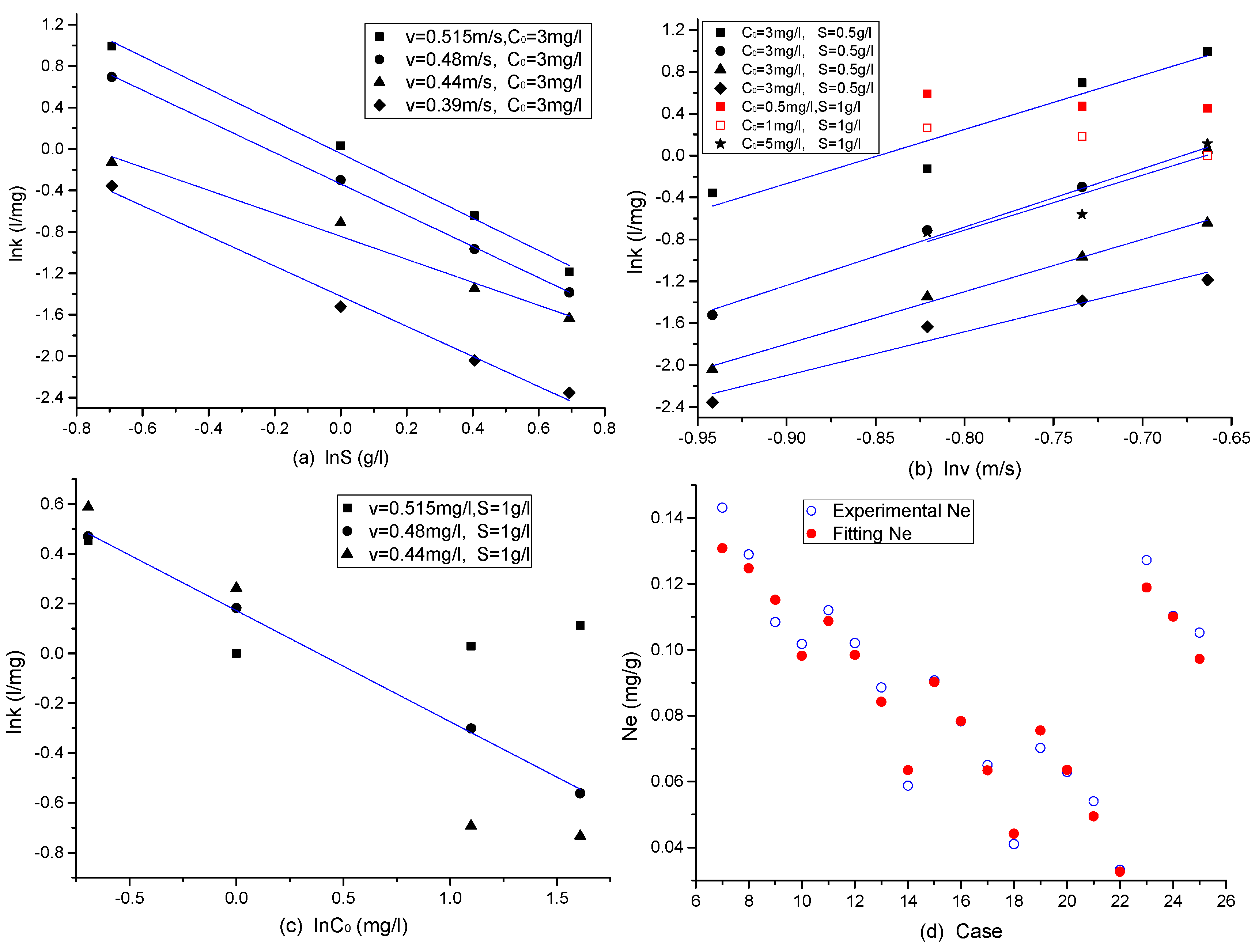
Firstly, in order to study the relationships between k and S, v, ${\mathrm{C}}_0$, the single factor analysis method is used. Samples of Figure 1a–c are obtained from the results of different physical experiments. All the blue lines are fitting values. The author analyzes the effect of every single factor by keeping the others same, such as the different S and equal v, ${\mathrm{C}}_0$. Figure 1a shows that the logarithms of k decrease monotonically as logarithms of S increase. Figure 1b shows that most of the logarithms of k increase linearly with the increase of logarithms of v apart from these red samples when ${\mathrm{C}}_0$ is smaller than 3 mg/L. In Figure 1c, it should be said that the fit is not very good. The R² based on all scattered points is 0.7. However, the R² based on cases of “v = 0.44 mg/L, S = 1 g/L” and “v = 0.48 mg/L, S = 1 g/L” are 0.96 and 0.99, respectively. While the R² based on the rest case of “v = 0.515 mg/L, S = 1 g/L” is small. The possible reason is that the corresponding physical experiment may have some errors. On the whole, we still think that the logarithms of k have a linear correlation with the logarithms of ${\mathrm{C}}_0$. Secondly, the multivariate nonlinear regression analysis method is used to obtain the comprehensive impact of all variables and get the Equation (1). Obviously, v and S are the major factors affecting k as their absolute exponential values are larger than 1.0, and ${\mathrm{C}}_0$ is the secondary factor. Figure 1d lists the original values of Ne from the physical experiments and the fitting values based on the Equation (1) with different cases except ${\mathrm{C}}_0$ = 0.5 and 1.0 mg/L. This is consistent with the literature [20]. The result shows that the fitting equation can be used in the next numerical simulation or even for further analysis.

$$k=\frac{{27\mathrm{v}}^{4.6}}{{\mathrm{C}}_0{}^{0.3}{\mathrm{S}}^{1.343}}-0.006$$

(1)

2.2.2. The Adsorption Coefficient $k_a$

Another important parameter in the adsorption-desorption process is $k_a$ which represents the speed of the reaction. By adopting the same method as above, the author analyzes the factors affecting $k_a$ and gives formula of $k_a$.

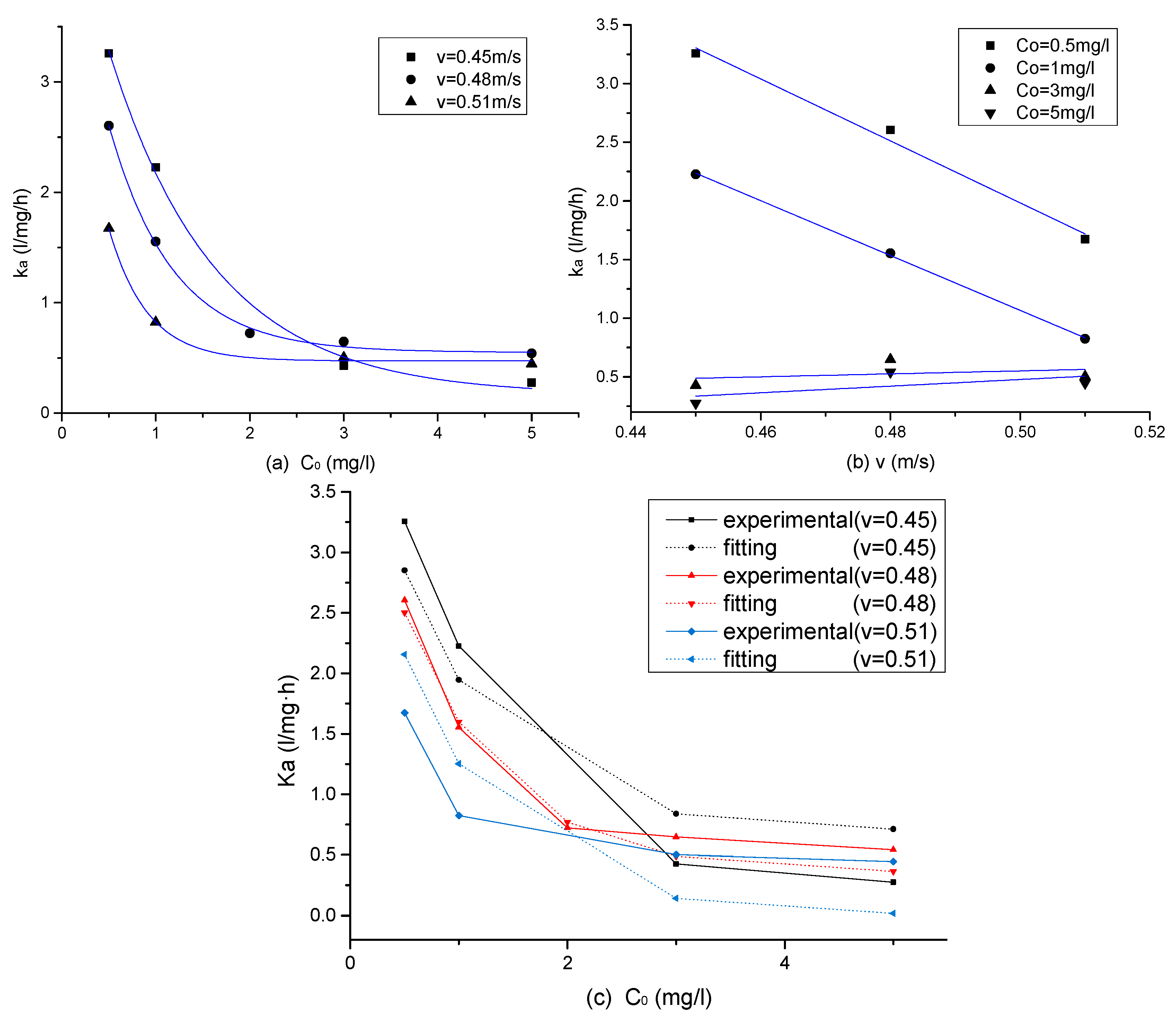
Firstly, in order to study the relationships between $k_a$ and v, ${\mathrm{C}}_0$, the single factor analysis method is used. Samples of Figure 2a,b are obtained from the results of different physical experiments when suspended sediment S equals to 1.0 g/L. All the blue lines are fitting values. The author uses the variable control approach to analyze the effect of every single factor, such as v and ${\mathrm{C}}_0$. In Figure 2a, there is a logarithmically decreasing trend of $k_a$ as the initial P concentration increases. Figure 2b shows that $k_a$ decreases linearly with the increase of velocity when the initial P concentrations were low, while the values of $k_a$ are similar at higher P concentrations. Secondly, the multivariate nonlinear regression analysis method is used to obtain the comprehensive impact of all variables and get the Equation (2). Obviously, both of v and S greatly affect $k_a$. Figure 2c lists the original values of $k_a$ from the physical experiments and the fitting values of $k_a$ from the Equation (1) with different cases. The R² based on all scattered points in Figure 2c is 0.88. This is consistent with the literature [10]. The result shows that the fitting equation can be used in the next numerical simulation or even for further analysis.

$$k_a=3.713{\mathrm{e}}^{-1.089{\mathrm{C}}_0}-11.584\mathrm{v}+5.909$$

(2)

2.3. Numerical Model

In the physical experiments, an elongated annular flume propelled by a Plexiglas gear is used to get a circulatory flow. While in the numerical model, a periodical numeric flume with the stream body force is built to get a constant and uniform flow. Based on Equations (1) and (2), the interaction between sediment and phosphorus is also considered. Then, the numerical model is built which consists of hydrodynamic module, sediment and phosphorus transport module.

2.3.1. Hydrodynamic Module

The three-dimensional hydrodynamic module is based on continuity Equation (3) and momentum Equation (4).

$$\nabla \cdot u=0$$

(3)

$$\frac{\partial u}{\partial t}+\left(u\cdot \nabla \right)u=-\frac{1}{\rho }\nabla p+\nu \cdot {\nabla }^{2}u+f$$

(4)

where u is the velocity vector, $\nabla$ is the Laplace operator, t is the time, p is the pressure, $\nu$ is the kinematic viscosity, which is equal to 10⁻⁶ m²/s at the normal temperature of 20 °C, and f is the body force, which is equal to the resultant force of the gravitational acceleration in the vertical direction and the stream body force, ${\mathrm{F}}_{\mathrm{x}}$. In order to get a constant and uniform water flow in the numerical study, a streamwise body force, ${\mathrm{F}}_{\mathrm{x}}$, is added to counteract the kinetic energy loss caused by resistances on solid boundaries and water viscosity.

2.3.2. Sediment Transport Module

The sediment transport is described using an equilibrium approach, assuming that all sediment are suspended in the given hydrodynamic condition. The governing equation can be written in Equation (5).

$$\frac{\partial \mathrm{S}}{\partial \mathrm{t}}+\frac{\partial (\mathrm{u}\mathrm{S})}{\partial \mathrm{x}}+\frac{\partial (\mathrm{v}\mathrm{S})}{\partial \mathrm{y}}+\frac{\partial (\mathrm{w}\mathrm{S})}{\partial \mathrm{z}}={\mathsf{\epsilon }}_{\mathrm{x}}\frac{{\partial }^2\mathrm{S}}{\partial {\mathrm{x}}^2}+{\mathsf{\epsilon }}_{\mathrm{y}}\frac{{\partial }^2\mathrm{S}}{\partial {\mathrm{y}}^2}+{\mathsf{\epsilon }}_{\mathrm{z}}\frac{{\partial }^2\mathrm{S}}{\partial {\mathrm{z}}^2}+\frac{\partial (\mathsf{\omega }\mathrm{S})}{\partial \mathrm{y}}$$

(5)

where S is the concentration of suspended sediment; t is time; x, y, z are coordinate directions, respectively; u, v, w are velocities of direction x, y, and z; ${\mathsf{\epsilon }}_{\mathrm{x}},{\mathsf{\epsilon }}_{\mathrm{y}},{\mathsf{\epsilon }}_{\mathrm{z}}$ are diffusion coefficient of direction x, y and z; $\mathsf{\omega }$ is the settling velocity.

2.3.3. Phosphorus Transport Module

Figure 3 shows a conceptual model of the phosphorus transport. The red circles represent dissolved or adsorbed phosphorus, the irregular khaki circles represent suspended sediment particles. Usually, the advection-diffusion equation is used for phosphorus transport to simulate the evolution processes of spatiotemporal concentration. By using the classical Langmuir equation (Equation (6)), the interaction of adsorption and desorption between dissolved phosphorus and adsorbed phosphorus is considered. Then the Equation (6) is added into the Advection-Diffusion equation (Equation (7)) as a source term which is shown in Equation (8).

$$\frac{\mathrm{d}\mathrm{N}}{\mathrm{d}\mathrm{t}}=k_a\cdot \mathrm{C}\cdot ({\mathrm{B}}_{\mathrm{m}}-\mathrm{N})-k_d\cdot \mathrm{N}$$

(6)

$$\frac{\partial \mathrm{N}}{\partial \mathrm{t}}+\mathrm{u}\frac{\partial \mathrm{N}}{\partial \mathrm{x}}+\mathrm{v}\frac{\partial \mathrm{N}}{\partial \mathrm{y}}+\mathrm{w}\frac{\partial \mathrm{N}}{\partial \mathrm{z}}={\mathrm{D}}_{\mathrm{x}}\frac{{\partial }^2\mathrm{N}}{\partial {\mathrm{x}}^2}+{\mathrm{D}}_{\mathrm{y}}\frac{{\partial }^{2}N}{\partial {\mathrm{y}}^2}+{\mathrm{D}}_{\mathrm{z}}\frac{{\partial }^2\mathrm{N}}{\partial {\mathrm{z}}^2}+{\mathrm{S}}^{\prime }$$

(7)

$$\{\begin{array}{l}\frac{\partial \mathrm{N}}{\partial \mathrm{t}}+\mathrm{u}\frac{\partial \mathrm{N}}{\partial \mathrm{x}}+\mathrm{v}\frac{\partial \mathrm{N}}{\partial \mathrm{y}}+\mathrm{w}\frac{\partial \mathrm{N}}{\partial \mathrm{z}}={\mathrm{D}}_{\mathrm{x}}\frac{{\partial }^2\mathrm{N}}{\partial {\mathrm{x}}^2}+{\mathrm{D}}_{\mathrm{y}}\frac{{\partial }^2\mathrm{N}}{\partial {\mathrm{y}}^2}+{\mathrm{D}}_{\mathrm{z}}\frac{{\partial }^2\mathrm{N}}{\partial {\mathrm{z}}^2}+k_a\cdot \mathrm{C}\cdot ({\mathrm{B}}_{\mathrm{m}}-\mathrm{N})-k_d\cdot \mathrm{N}\\ \frac{\partial \mathrm{C}}{\partial \mathrm{t}}+\mathrm{u}\frac{\partial \mathrm{C}}{\partial \mathrm{x}}+\mathrm{v}\frac{\partial \mathrm{C}}{\partial \mathrm{y}}+\mathrm{w}\frac{\partial \mathrm{C}}{\partial \mathrm{z}}={\mathrm{D}}_{\mathrm{x}}\frac{{\partial }^2\mathrm{C}}{\partial {\mathrm{x}}^2}+{\mathrm{D}}_{\mathrm{y}}\frac{{\partial }^2\mathrm{C}}{\partial {\mathrm{y}}^2}+{\mathrm{D}}_{\mathrm{z}}\frac{{\partial }^2\mathrm{C}}{\partial {\mathrm{z}}^2}-(k_a\cdot \mathrm{C}\cdot ({\mathrm{B}}_{\mathrm{m}}-\mathrm{N})-{\mathrm{k}}_{\mathrm{d}}\cdot \mathrm{N})\cdot \mathrm{S}\end{array}$$

(8)

where N is the adsorbed phosphorus amount per unit mass by sediment (mg/g); C is the concentration of dissolved P in the water (mg/L); t is time; ${\mathrm{S}}^{\prime }$ is the source term; S is sediment concentration (g/L);$k_a$, $k_d(=k_a/k)$ are separately the coefficients of the adsorption and the desorption (l/mg/h, 1/h); ${\mathrm{B}}_{\mathrm{m}}$ is the maximum adsorption of adsorption (mg/g).

3. Model Verification

3.1. Hydrodynamic

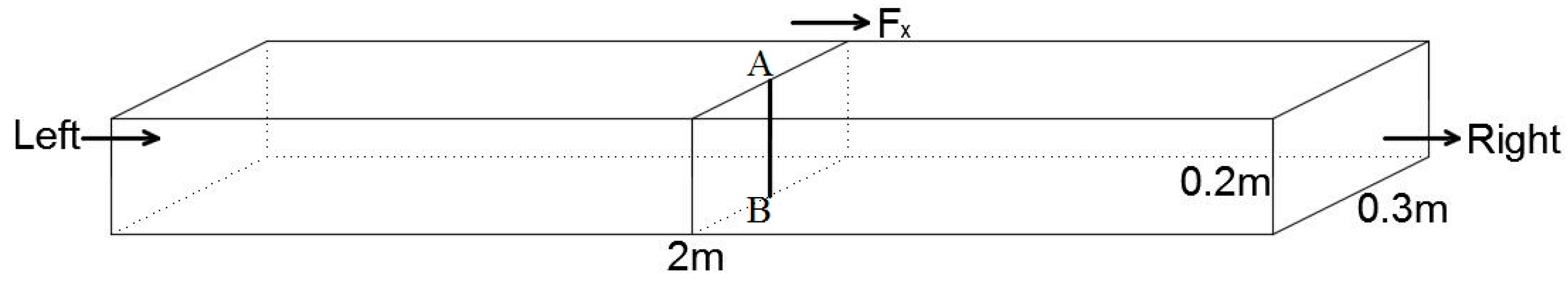
As is demonstrated in Figure 4, a periodical numerical flume is built to simulate the flume of the previous physical experiment where the recirculating water is propelled by Plexiglas gear driven by an AC frequency conversion electric machine. In order to get a constant and uniform water flow in the numerical study, a streamwise body force, ${\mathrm{F}}_{\mathrm{x}}$, is added to counteract the kinetic energy loss caused by resistances on solid boundaries and water viscosity.

The numerical simulation is designed in a 2 m × 0.3 m × 0.2 m (L × W × H) periodical numerical flume, and the resolution of computational grids is 200 × 30 × 20, which is sufficiently fine to obtain a stable numerical solution. The velocities after the flow of laboratory experiment reaching a steady state are used as the initial condition of the numerical simulation. The initial fluid level of all different cases is 0.2 m. All the solid walls including the sidewalls and the flume bed are considered as the no-slip wall boundary conditions. In this study, the turbulence is predicted by the renormalization group (RNG) $\mathrm{k}-\mathsf{\epsilon }$ turbulent model (turbulent kinetic energy k and its dissipation ratio $\mathsf{\epsilon }$).

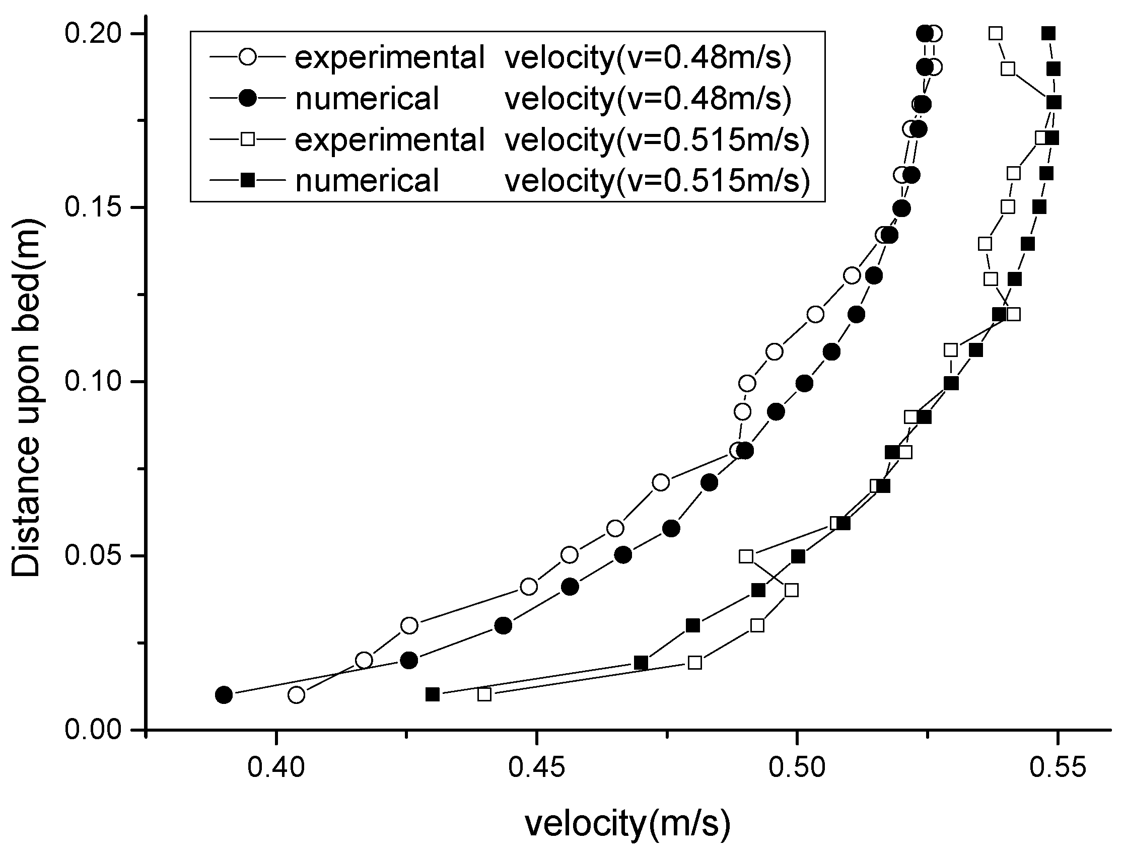
To compare the numerical and experimental hydrodynamic conditions, two cases are set with the mean cross-sectional velocities of 0.515 m/s and 0.48 m/s, respectively. Shown in Figure 5, the streamwise velocities along the water depth at the bold black line AB (Figure 4) of these two cases are in good agreement with experimental velocities.

3.2. Sediment and Phosphorus Transport

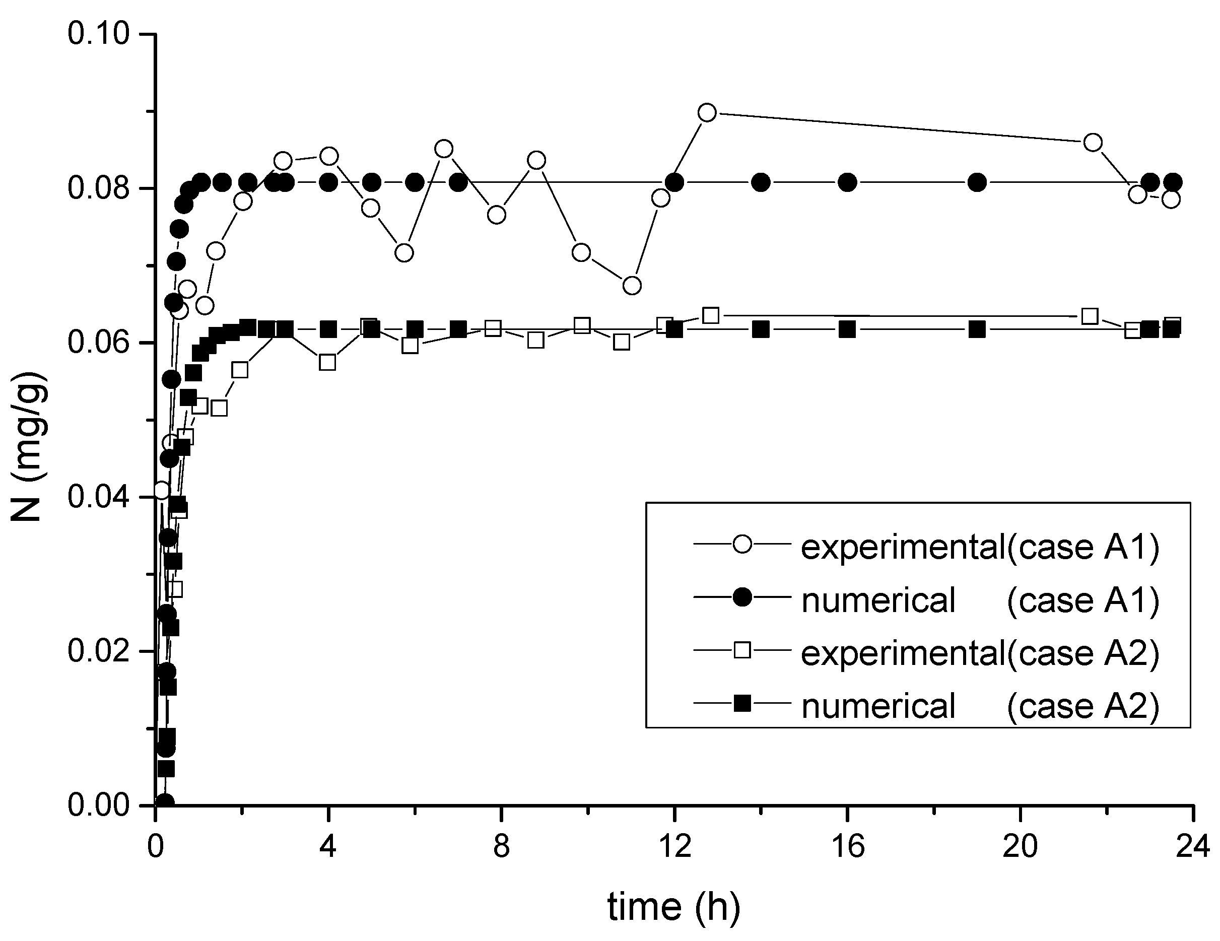
According to the result of the batch reactor experiments [10], the maximum adsorption of adsorption ${\mathrm{B}}_{\mathrm{m}}$ is 0.15 mg/g. The initial phosphorus concentration and sediment concentration equal to that of the corresponding physical experiments are given in

Table 2. The initial phosphorus concentration C₀, initial sediment concentration S, and the cross-sectional average velocity v of different cases in the numerical simulations.

Case	C0 (mg/L)	S (g/L)	v (m/s)
A1	0.5	1	0.515
A2	1	1	0.515

. The variation of adsorbed phosphorus amount per unit mass sediment with time is shown in Figure 6. Although the experimental N changes a little around numerical results, the values of them are almost the same when reaching an equilibrium state.

4. Model Application

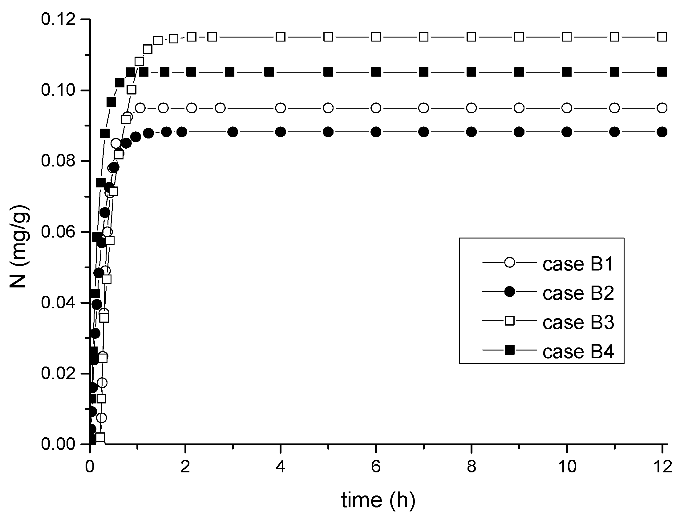
In order to further study the interaction processes between phosphorus and sediment, another four cases are considered (listed in

Table 3. The initial phosphorus concentration C₀, initial sediment concentration S, and the cross-sectional average velocity v of different cases in the numerical simulations.

Case	C0 (mg/L)	S (g/L)	v (m/s)
B1	2	1	0.515
B2	2	1	0.48
B3	4	1	0.515
B4	4	1	0.48

). Derived k and $k_a$ based on Equation (1) and (2) are applied to new cases (B1–B4). Figure 7 shows the variation of the amount of adsorbed phosphorus amount per unit mass sediment with time for a sediment concentration of 1 g/L with different initial P concentrations. Obviously, N reaches to a stable state different from dynamic equilibrium of the physical experiment after several hours because Equation (5) is used to consider the interaction in the numerical simulation. N increases with the initial phosphorus concentration by comparing of A1, A2, B1 and B3 from Figure 6 and Figure 7. And N also increases with the velocity by comparing B1 and B2 or B3 and B4.

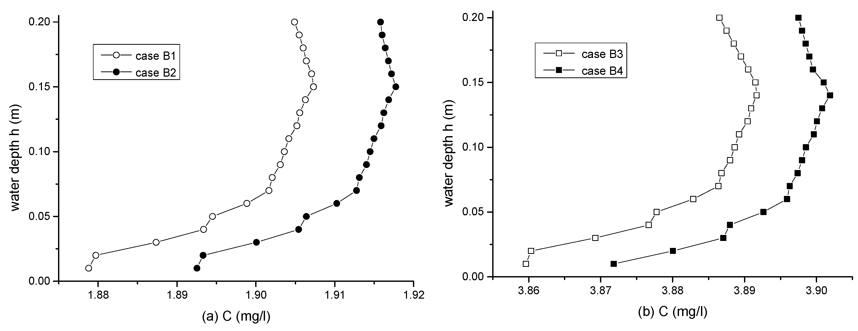
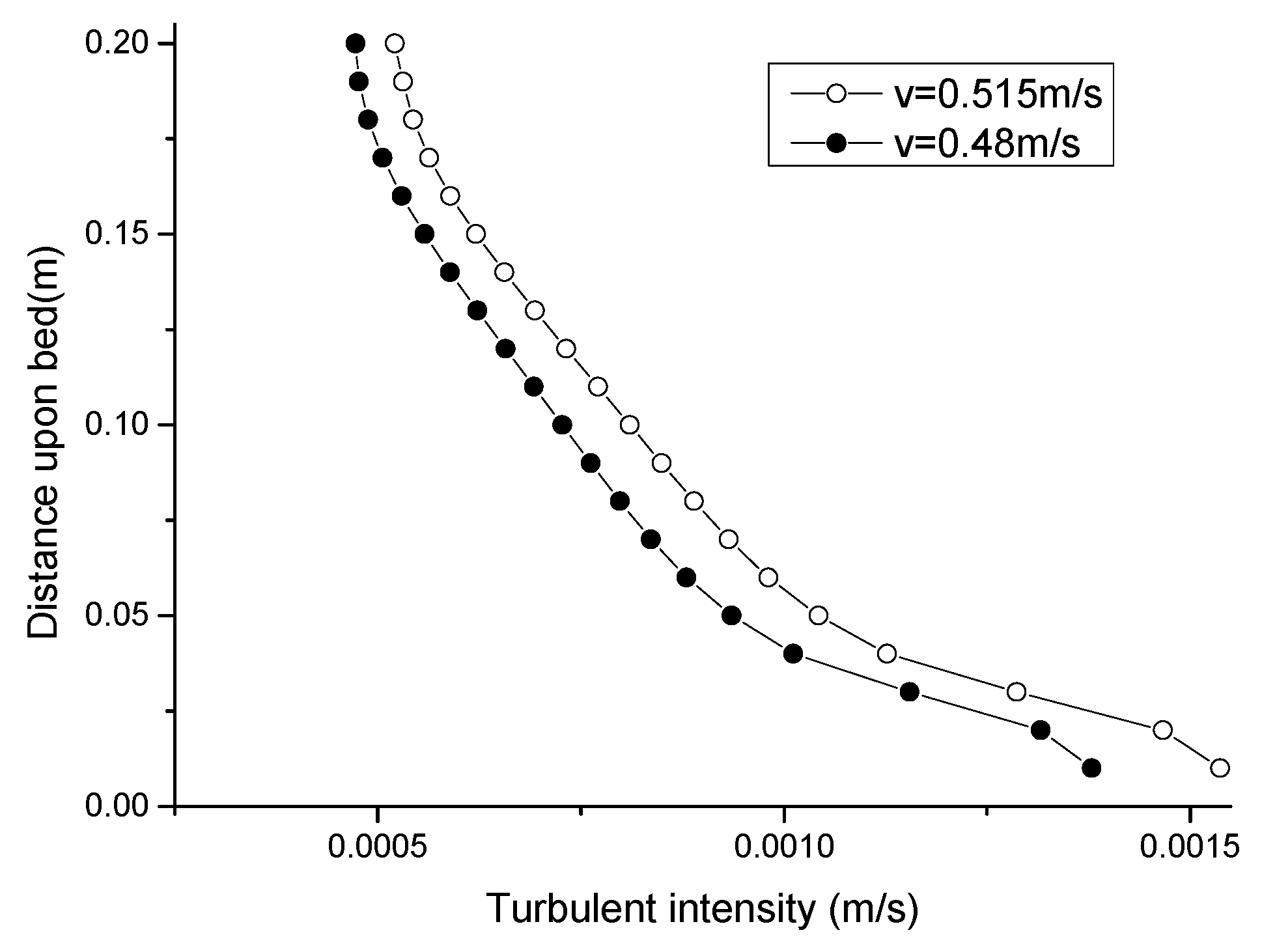
Figure 8 shows that the concentration of dissolved phosphorus in the water changes little within the whole water depth and its maximum approximately appears in the 3/4 water depth. One reason is that the strong turbulence intensity of the water flow and the high sediment concentration at the bottom of the tank can result in the large amount of phosphorus absorbed by the sediment (shown in Figure 9). Another is that the large flow rate of the upper water body leads to the increase of the adsorption of phosphorus by sediment (Figure 5). So in the final upper water body and the lower water body, the amount of dissolved phosphorus in the water is relatively low, and the concentration of phosphorus in the 3/4 water depth shows a relatively large value. In stable natural rivers or reservoirs, dissolved phosphorus shows an increasing trend from the bottom to the surface of the water. However, this is not always the case. Both sediment and hydrodynamic forces can cause changes in the distribution of dissolved phosphorus along the depth.

5. Conclusions

In this paper, a numerical model of hydrodynamics, sediment, and phosphorus based on improved Langmuir equation was established where the processes of adsorption and desorption were considered. The main conclusions can be summarized as follows:

(1)

The influence of both hydraulic and environmental factors on phosphorus sorption to suspended sediments was quantitatively investigated by fitting analysis of $k_a$, and the ratio k between the adsorption coefficient and the desorption coefficient in flume experiments.

(2)

The concentration of dissolved phosphorus was unevenly distributed along the depth, and the maximum value approximately appeared in the 3/4 water depth because both the high velocity in the top layer and the high turbulence intensity in the bottom layer can promote sediment adsorption on phosphorus.

(3)

Derived k and $k_a$ based on equation can well be applied to new cases. However, it would be much more meaningful to establish a general formula for k based on a large quantity of experiments with sediment of different origins.

(4)

This paper hasn’t taken bed sediment into consideration. However, bed sediment widely exists in natural rivers and has great impaction on the adsorption and desorption of phosphorus. So the next step is to further consider the sedimentation and suspension between suspended sediment and bed sediment, and the adsorption and phosphorus processes in the bed sediment layer.

(5)

Natural rivers are very different from experimental flumes because of complex terrain and hydrodynamic conditions. So, it is of great importance to build a model based on typical riverbed and real dynamic conditions with the data of on-site water samples and sand samples, especially in the river seriously affected by eutrophication.

References

- Schindler, D.W. Recent advances in the understanding and management of eutrophication. Limnol. Oceanogr. 2006, 51, 356–363. [Google Scholar] [CrossRef] [Green Version]
- Huang, L.; Fang, H.W.; Reible, D. Mathematical model for interactions and transport of phosphorus and sediment in the Three Gorges Reservoir. Water Res. 2015, 85, 393–403. [Google Scholar] [CrossRef] [PubMed]
- Fang, H.W.; Chen, M.H.; Chen, Z.H.; Zhao, H.M.; He, G.J. Effects of sediment particle morphology on adsorption of phosphorus elements. Int. J. Sediment Res. 2013, 28, 246–253. [Google Scholar] [CrossRef]
- Withers, P.J.; Jarvie, H.P. Delivery and cycling of phosphorus in rivers: A review. Sci. Total Environ. 2008, 400, 379. [Google Scholar] [CrossRef] [PubMed]
- Kalnejais, L.H.; Martin, W.R.; Bothner, M.H. The release of dissolved nutrients and metals from coastal sediments due to resuspension. Mar. Chem. 2010, 121, 224–235. [Google Scholar] [CrossRef]
- House, W.A.; Denison, F.H.; Armitage, P.D. Comparison of the uptake of inorganic phosphorus to a suspended and stream bed-sediment. Water Res. 1995, 29, 767–779. [Google Scholar] [CrossRef]
- Xiao, Y.; Lu, Q.; Cheng, H.K.; Zhu, X.L.; Tang, H.W. Surface properties of sediments and its effect on phosphorus adsorption. J. Sediment Res. 2011, 6, 64–68. [Google Scholar]
- Zhou, A.; Tang, H.; Wang, D. Phosphorus adsorption on natural sediments: Modeling and effects of pH and sediment composition. Water Res. 2005, 39, 1245–1254. [Google Scholar] [CrossRef] [PubMed] [Green Version]
- Wang, S.; Jin, X.; Bu, Q.; Jiao, L.; Wu, F. Effects of dissolved oxygen supply level on phosphorus release from lake sediments. Colloids Surf. A Physicochem. Eng. Asp. 2008, 316, 245–252. [Google Scholar] [CrossRef]
- Li, Z.W.; Tang, H.W.; Xiao, Y.; Zhao, H.Q.; Li, Q.X.; Ji, F. Factors influencing phosphorus adsorption onto sediment in a dynamic environment. J. Hydroenviron. Res. 2016, 10, 1–11. [Google Scholar] [CrossRef]
- Xia, B.; Zhang, Q.H.; Jiang, C.B.; Nie, X.B. Experimental investigation of effect of flow turbulence on phosphorus release from lake sediment. J. Sediment Res. 2014, 212–213, 299–306. [Google Scholar]
- Park, R.A.; Clough, J.S.; Wellman, M.C. AQUATOX: Modeling environmental fate and ecological effects in aquatic ecosystems. Ecol. Model. 2008, 213, 1–15. [Google Scholar] [CrossRef]
- Broshears, R.E.; Clark, G.M.; Jobson, H.E. Simulation of stream discharge and transport of nitrate and selected herbicides in the Mississippi River Basin. Hydrol. Process. 2001, 15, 1157–1167. [Google Scholar] [CrossRef]
- Chu, X.; Rediske, R. Modeling Metal and Sediment Transport in a Stream-Wetland System. J. Environ. Eng. 2012, 138, 152–163. [Google Scholar] [CrossRef]
- Jalali, M.; Peikam, E.N. Phosphorus sorption-desorption behaviour of river bed sediments in the Abshineh river, Hamedan, Iran, related to their composition. Environ. Monit. Assess. 2013, 185, 537–552. [Google Scholar] [CrossRef] [PubMed]
- Song, L.X. Study on Nutrients Output Change Law from Non-Point Source in Xiangxi Basin of the Three Gorges Reservoir. Ph.D. Thesis, Wuhan University, Wuhan, China, 2011. [Google Scholar]
- Yin, J.; Deng, C.; Yu, Z.; Wang, X.; Xu, G. Effective Removal of Lead Ions from Aqueous Solution Using Nano Illite/Smectite Clay: Isotherm, Kinetic, and Thermodynamic Modeling of Adsorption. Water 2018, 10, 210. [Google Scholar] [CrossRef]
- Pavlatou, A.; Polyzopoulos, N.A. The role of diffusion in the kinetics of phosphate desorption: The relevance of the Elovich equation. Eur. J. Soil Sci. 1988, 39, 425–436. [Google Scholar] [CrossRef]
- Huang, S.L.; Wan, Z.H. Study on sorption of heavy metal pollutants by sediment particles. J. Hydrodyn. Ser. B 1997, 9, 9–23. [Google Scholar]
- Tang, H.W.; Zhao, H.Q.; Li, Z.W.; Yuan, S.Y.; Li, Q.X.; Ji, F.; Xiao, Y. Phosphorus sorption to suspended sediment in freshwater. In Water Management; Thomas Telford Ltd.: London, UK, 2016. [Google Scholar]
Figure 1.
Relationships between k and S, v, (a–c) and the comparison between the fitting and experimental ratio Ne with cases 7–25 (d).
Figure 2.
Relationships of and v, (a,b) and the comparison between the fitting and experimental ratio with different cases (c).
Figure 3.
Conceptual model of the phosphorus transport (the red circles represent dissolved or adsorbed phosphorus, the irregular khaki circles represent suspended sediment particles).
Figure 4.
Schematic diagram of the periodical numerical flume.
Figure 5.
Comparison between the numerical and experimental streamwise velocity at the line AB with two cases of cross-sectional average velocity 0.48 and 0.515 m/s.
Figure 6.
Variation of the adsorbed phosphorus amount per unit mass sediment with time and the comparison between numerical and experimental value of case A1 and A2.
Figure 7.
Variation of the adsorbed phosphorus amount per unit mass sediment with time of case B1–B4.
Figure 8.
Variation of the concentration of dissolved P in the water of case B1–B4 at an equilibrium state.
Figure 9.
Comparison of the turbulent intensity distribution along the water depth with two cases of cross-sectional average velocity 0.48 and 0.515m/s.