Geostatistical Characterization of the Transmissivity: An Example of Kuwait Aquifers


1
Environment and Life Sciences Research Center, Kuwait Institute for Scientific Research, Safat 13109, Kuwait
2
Desert and Arid Zones Sciences Program Arabian Gulf University, Manama P.O. Box 26671, Bahrain
*
Author to whom correspondence should be addressed.
Water 2018, 10(7), 828; https://doi.org/10.3390/w10070828
Submission received: 11 March 2018
/
Revised: 22 May 2018
/
Accepted: 28 May 2018
/
Published: 22 June 2018
(This article belongs to the Section Hydrology)
Abstract
:Management of groundwater resources is critical to arid countries like Kuwait. One crucial information that is often not available to groundwater modelers is transmissivity of aquifers. Kriging is used to characterize the transmissivity of the two most commonly used aquifers in Kuwait (the Dammam and Kuwait Group aquifers). The transmissivity of the two aquifers is represented as a random spatial function where heterogeneity is described by the probability distribution and variogram of sample values. A structural analysis was performed which consisted of the construction and interpretation of sample variograms and the selection of model variograms to best fit the structure of the log-transformed transmissivity. The analysis indicated that the transmissivity of the Dammam aquifer is highly anisotropic and has a longer range of influence and larger variance (39 km; 333,487) than those for the Kuwait Group aquifer (10 km; 44,613). The model variograms were used in the kriging analysis to estimate the spatial average value of the transmissivity of the two aquifers in Kuwait. The estimated transmissivity of the Kuwait Group aquifer ranges from <50 to about 800 m2 day−1, and is controlled principally by the thickness of the saturated zone in the aquifer. The estimated transmissivity in Dammam aquifer ranges from ~100 to 2200 m2 day−1, with high transmissivity fields coinciding with both the areas of major anticline and fault structures and the areas of aquifer recharge by fresh water, indicating the enhancement of the transmissivity on these structures by dissolution. Low transmissivity fields are located in the areas where the aquifer waters are stagnant. The performed analysis can be used to aid in the development of numerical models for sustainable management of the aquifer system in Kuwait, defining artificial recharge sites, and in optimizing the locations of future development wellfields.
1. Introduction
Transmissivity (T) is often used in specifying the groundwater extraction potential of an aquifer [1]. Hence, estimating the T is considered an essential parameter for developing local and regional water management plans, modeling groundwater flow and solute transport [2], and selecting areas for additional hydrologic tests [3]. Transmissivity depends both on the properties of the porous matrix and the fluid passing through the strata. A pumping test is the most reliable and standard method to determine the T value in aquifers. However, these pumping tests are expensive, and often, their results are localized spatially. This makes it imperative to extrapolate the information on a larger scale for developing sustainable water management plans. The geostatistical techniques are the most widely used for extrapolation of the measured values to a broader spatial domain [4]. Kriging is a widely applied approach in hydrology [5,6,7]; It is a stochastic approach for determining parameters at unknown points.
In Kuwait, large-scale wellfield development was initiated by the Ministry of Electricity and Water (MEW), and the Kuwait Oil Company (KOC) in the 1960s, for which T values were determined. However, the water needs of Kuwait are steadily increasing [8], both with the growth in population, and increasing per capita consumption that has gone up from 113 L day−1, in 1970, to 464 L day−1 in 1998 [9], and over 485 L day−1 in 2015. More wellfields are required to meet the water demand, making it imperative to develop regional groundwater models that, in turn, need a reliable T value on a broader spatial domain.
This paper outlines the effectiveness of kriging in the large-scale extrapolation of transmissivities. This case study highlights, as an example, the two principal aquifers in Kuwait, i.e., Kuwait Group aquifer and Dammam aquifer. Mapping T will aid in the optimum development of groundwater and wellfield management; i.e., understanding the flow system and flow patterns, optimizing placement of development wells, selecting areas for artificial recharge, and conducting numerical modeling studies.
2. Materials and Methods
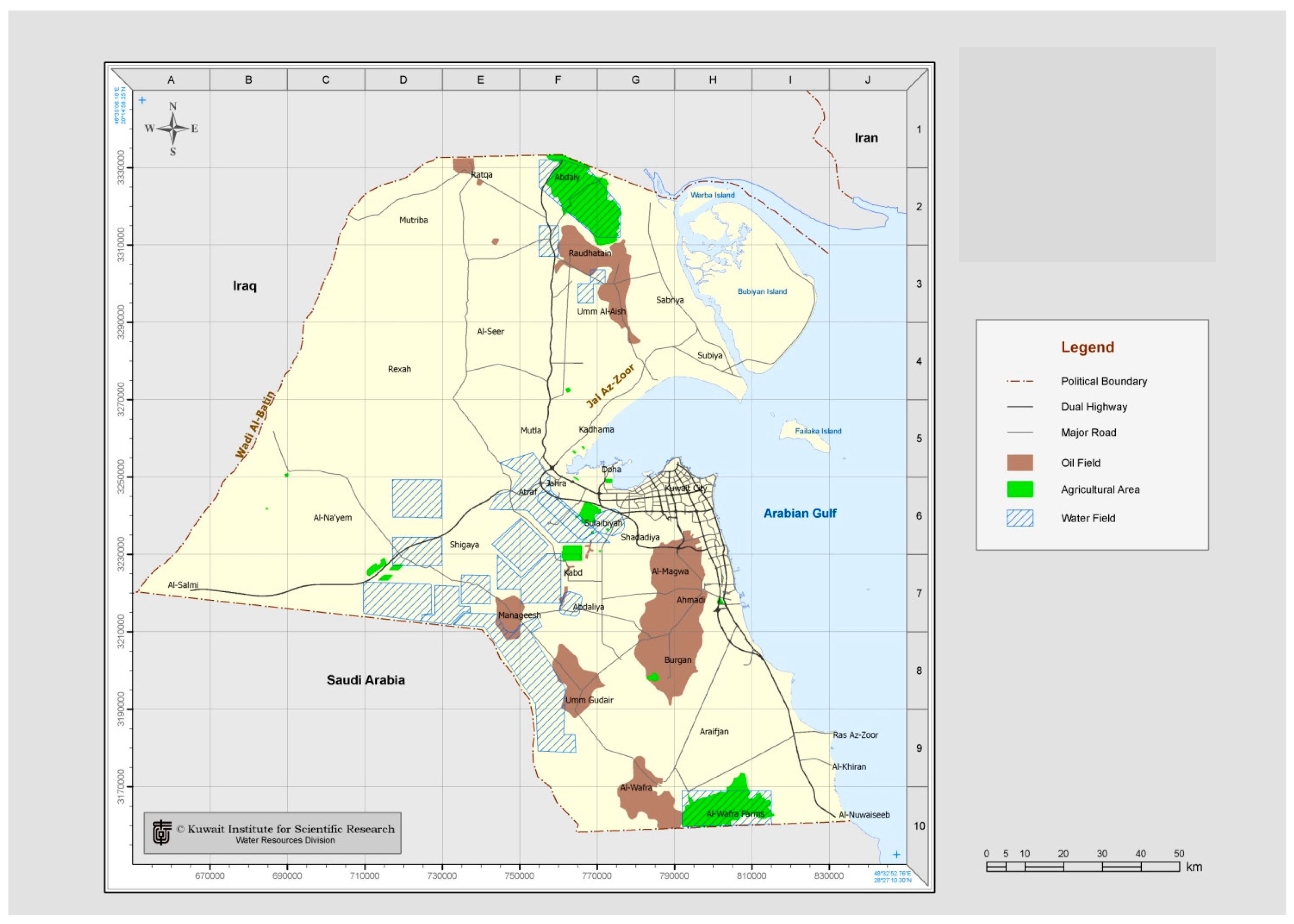
Kuwait is located on the northwestern side of Arabian Gulf, with Kingdom of Saudi Arabian in the south and west and Iraq in north and west quadrant (Figure 1).
2.1. Geohydrology
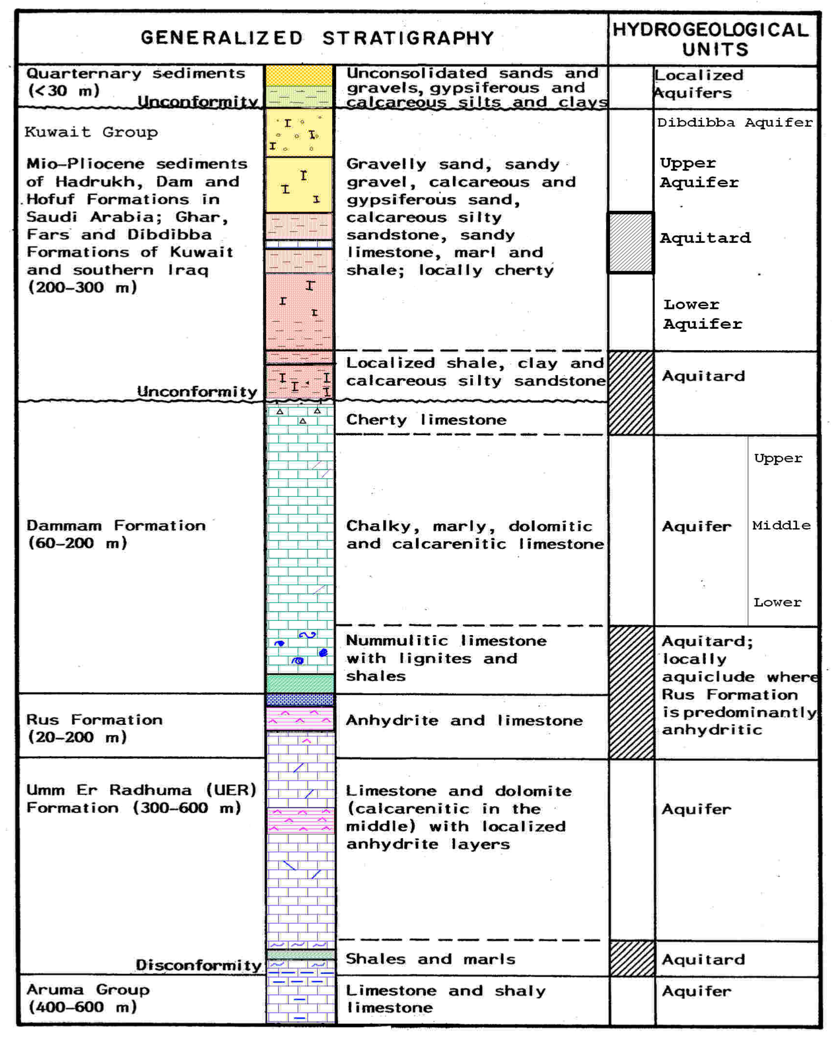
Kuwait forms part of the hyper-arid region, with brackish groundwater as the only source of natural potable water. The country obtains its required supply of groundwater from two principal aquifers, i.e., Dammam (Dm) and Kuwait Group (Kg) through established wellfields (Figure 1). The Dm aquifer is developed in the chalky and dolomitic limestone unit, of the middle part of the Dammam Formation (Middle Eocene), and occurs under confining conditions across most of Kuwait (Figure 2). The thickness of Dm Formation is from 60 m to 200 m in the northern part of Kuwait. The potentiometric aquifer surface (in the initial stage) varies from about 100 m above sea level in the extreme southwest of Kuwait to a few meters near the eastern coast, with a relatively gentle pre-development gradient (before 1970) of about 0.8 m km−1 [11]. The direction of groundwater flow is generally towards the east and northeast. Water quality distribution in the Dm aquifer follows its potentiometric trends typically; the total dissolved solids (TDS) increase from ~2500 mg L−1 in the southwestern areas of Kuwait to ~40,000 mg L−1 near the coast and Kuwait Bay, to >100,000 mg L−1 in northeastern Kuwait. The zone to the northeast, where the TDS values exceed those found in seawater, represents a non-flushed portion of the aquifer filled with connate water [12,13].
The Kg aquifer is developed in the unconsolidated gravel and sand units of the Kuwait Group of Miocene–Pleistocene age and occurs under unconfined conditions throughout Kuwait. Although the upper and lower permeable units of the Kg are separated at places by a semi-pervious sequence of silt, sand, and clay layers (Figure 2), the entire sequence is considered as one hydrographic unit for the aquifer development. The saturated thickness of the aquifer ranges from zero at the southwestern corner of Kuwait, where the aquifer is dry, to over 300 m to the northeast. This general trend in the saturated thickness is interrupted by localized reductions in the coastal areas of the anticlines, and in some areas, complete desaturation (structures at southeast and east of Kuwait). The potentiometric surface of the Kg aquifer follows closely that of the Dm aquifer, and hence, its flow direction. However, the potentiometric values in the former are lower by about 5 m, with head differences increasing towards the coastal area. The Kg aquifer contains water similar in quality to that of the Dm aquifer [14], and ranges from ~3000 mg L−1 in the southwest to ~130,000 mg L−1 in the northeast over a distance of about 150 km [15].
A layer of cherty limestone unit ranging in thickness from 1.5 to 30 m overlying the top of Dm aquifer and clay, averaging 10 m thick, separates the Kg and Dm aquifers (Figure 2). The entire hydrologic system in Kuwait is bounded on the top by the water table of the Kg aquifer, and on the base by the relatively impermeable nummulitic limestone with lignites and shale intercalations of the Dammam Formation, along with the underlying massive anhydrides (20–200 m) of the Rus Formation (Lower Eocene).
2.2. Transmissivity Data Sets
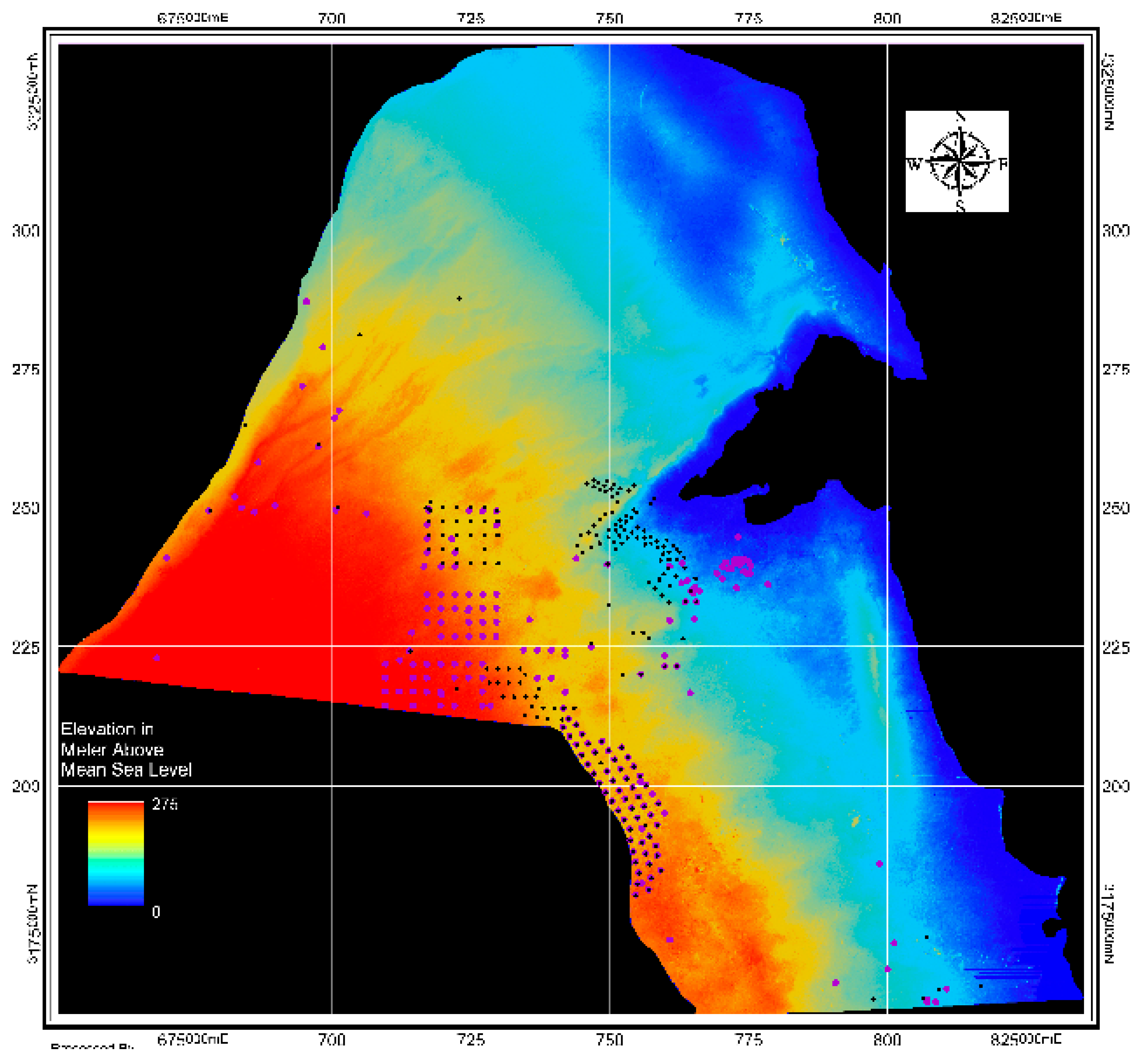
Transmissivity data for the Dm and Kg aquifers were obtained from the Ministry of Electricity and Water (MEW), Kuwait. MEW has a record of aquifer tests conducted in wellfields in Kuwait in addition to a number of exploration wells (Figure 3). The data set consists of 206 measurements for the Dm aquifer and 216 measurements for the Kg aquifer. For both aquifers, transmissivity data used in this study are for those conducted in fully penetrating wells. The transmissivity data are usually reported in imperial gallons per day per foot (Ig day−1 ft−1), and were converted to square meter per day (m2 day−1) units.
The two units of Kg aquifer (upper and lower) are considered as one hydrostratigraphic unit for the aquifer development, and most of the pumping tests conducted in the aquifer have been carried out with screened intervals covering both the units, and T is an average of the two units.
2.3. Statistical Analysis
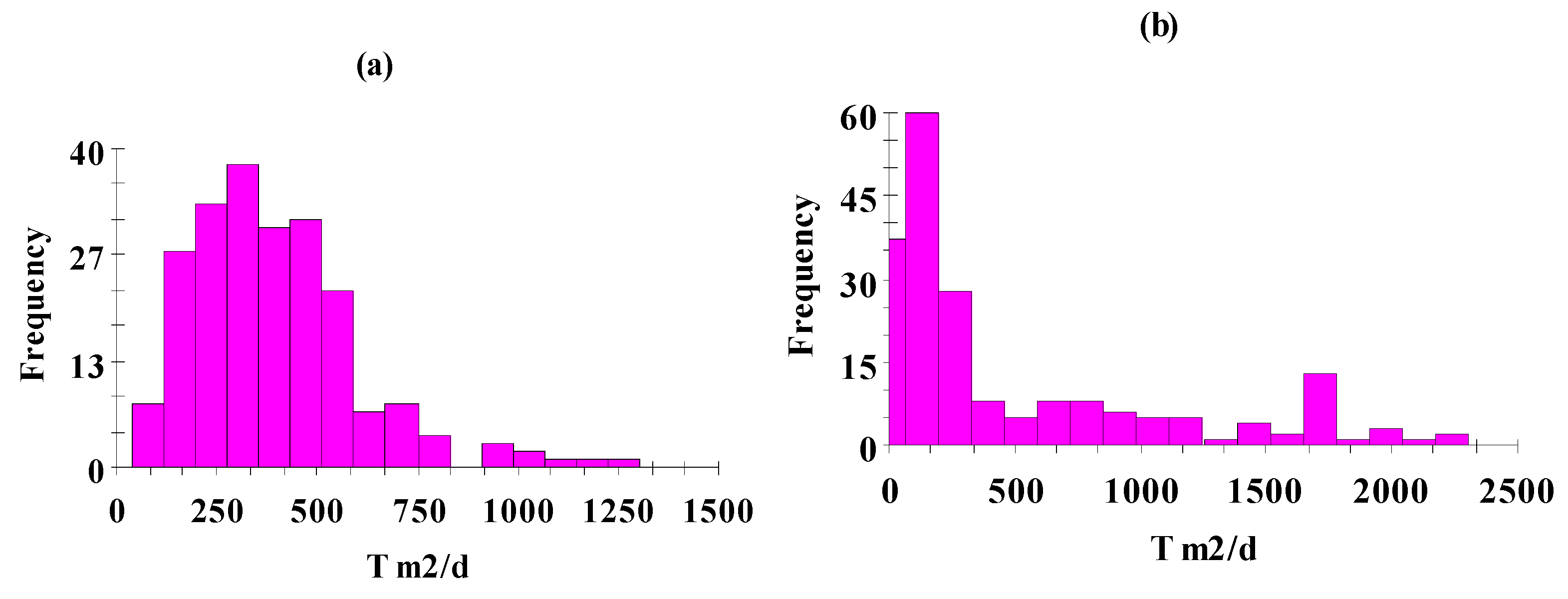
The T data were statistically analyzed, after cleaning the data of the outliers, following the procedure suggested by Woodbury and Sudicky [17]. The three outliers from Kg aquifer and four from Dm aquifer where the T values were <20 m2 day−1 were not considered in statistical analyses. A single value of >4500 m2 day−1 for Dm aquifer was also omitted from statistical analyses. This approach of Woodbury and Sudicky seems to provide more realistic results in both determining population statistics and variogram estimation. Table 1 presents a comparison of the corresponding statistics for the T in the two aquifers. T of Dm aquifer has a higher mean and higher variance compared to the Kg aquifer. The higher variation in T of the Dm aquifer is indicative of the karst within this aquifer.
The histogram of Kg and Dm aquifers appears to be moderately skewed to the right (Figure 4a,b), as indicated by the values of the coefficient of skewness. The two histograms indicate marked asymmetry, especially the Dm aquifer, with tails towards the higher values of transmissivity, suggesting log-normal distribution. This behavior for transmissivity histograms appears to be consistent with those observed in geostatistical transmissivity studies elsewhere [5,17,18,19,20].
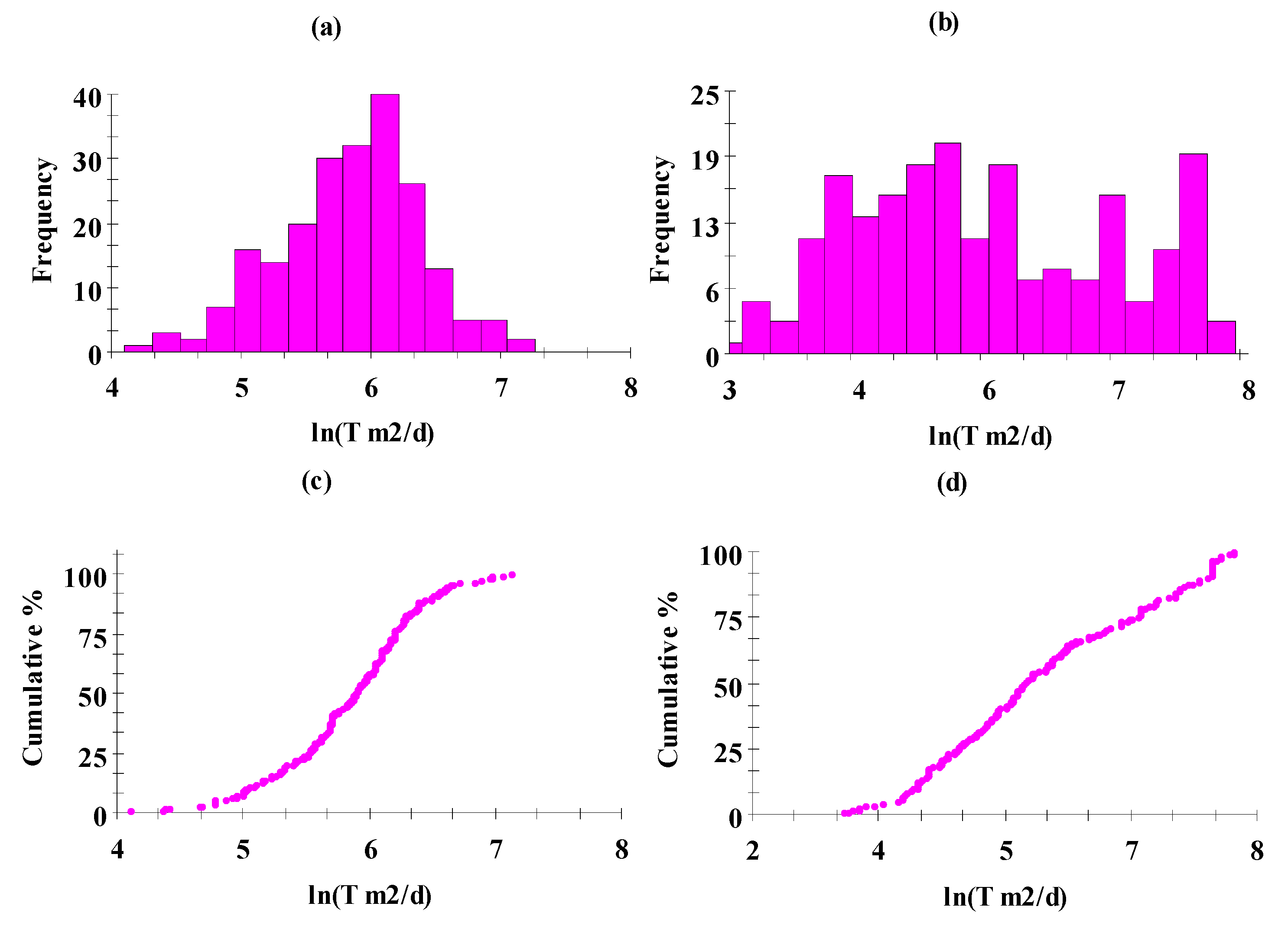
In this study, the logarithm of the data was considered for geostastical analyses, the T for any unknown location was then extrapolated by merely taking the exponential of the estimated value; this approach was successfully used in earlier studies [19,21]. The variogram shows a better correlation with the measured values [22]. The approach was tested for both Kg and Dm aquifers (Figure 5a,b). The percentage cumulative frequency distribution shows a reasonable correlation with a straight line (normality condition), in spite of the fact that this data was skewed, indicating validity of the use of log transformed T.
2.4. Structural Analysis
The estimation of the sample semivariogram and selection of an appropriate theoretical semivariogram is the fundamental basis of any geostatistical analysis [23]. Semivariograms describe the spatial correlation structure of the regionalized variables, which is defined as
where γ(h) is the variogram function, and Z(x) and Z(x + h) are two of the random variables comprising the random field. The random field is assumed to satisfy the intrinsic hypothesis; i.e., the difference [Z(x) − Z(x + h)] is second-order stationary, meaning that its mean function is constant, and its covariance function depends only on the separation distance h (Olea, 1984; Philip and Kitanidis, 1989).
The experimental variogram and the theoretical model of the log(T) of both aquifers were computed by using the GS+ Geostatistics for the Environmental Sciences version 7.0, 2004.
2.5. Experimental Variogram
There are numerous methods that are used for computation of the experimental variogram including: the “classical” estimator [24], the Cressie–Hawkins estimator [25], the squared median of the absolute deviation (SMAD) estimator [26], and Omre estimator [27]. In this study, we have used the classical estimator for calculating the experimental variogram after screening outliers from the database, as suggested by Woodbury and Sudicky [17].
The classical estimator equation is [22]
where n(h) is the number of data pairs separated by the vector, or lag distance, h, and Z(xi) are measured values of log transmissivity at coordinates xi. The estimator γ(h) is the experimental variogram. The classical estimator is an optimal estimator of the variogram, provided that the pairs Z(xi) and Z(xi + h) are bivariate normal and independent.
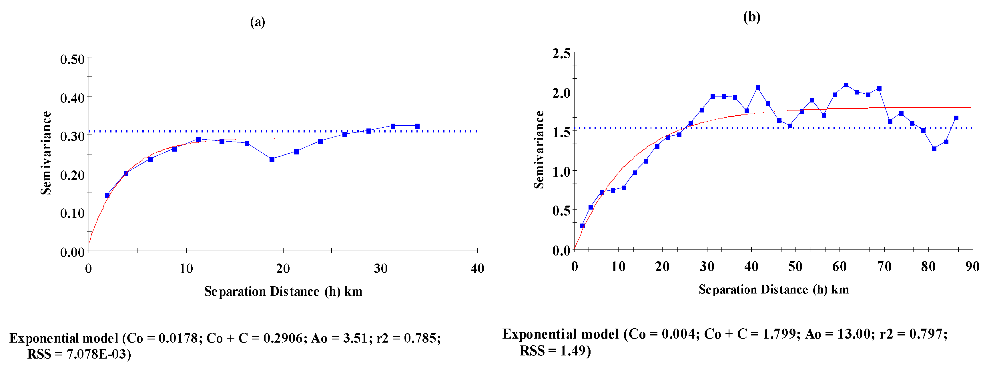
The experimental semivariogram for specified distances and direction were obtained for both the Kg and Dm aquifers (Figure 6a,b) utilizing an approach proposed by Istok et al. [28]. The experimental variogram for the two aquifers shows a clear sill, and the presence of spatial correlation at the shortest lag.
2.6. Model Semivariogram
The exponential model was used to fit the experimental variogram for both Kg and Dm aquifers. An iterative process was applied to determine the optimum length of the variogram, by reducing the lag distance, which is the range of the maximum and minimum distance between points over which the experimental variogram is calculated. The lag distance was reduced from 50.0 km to 25.0 for Kg, and from 90.0 km to 45.0 km for Dm aquifer. A regular lag class distance interval was also systematically reduced, from 6.0 km to 1.5 km, with each active lag distance for both aquifers. The exponential models were found to be more applicable for both aquifers. The simple exponential model equation used was as follows [29]:
where C0 is the nugget variance, and C0 + C the sill. C0 and C represent the random and spatial components of variation, respectively, a0 is the model’s range parameter, which is distinguished form a, the range of influence, or the separation distance over which spatial dependence is apparent, for the exponential model a, equals 3a0.
The residual sums of squares (RSS), r2, and proportion C/(C0 + C) were used to select the fitted model. The proportion C/(C0 + C), is the proportion of the spatially structured variance (C) to the sample variance (C0 + C). This value will be 1.0 for a variogram with no nugget variance (where the curve passes through the origin); conversely, it will be 0.0, where there is no spatially dependent variation at the range specified, i.e., where there is a pure nugget effect. Table 2 lists the fitted parameters to the experimental variogram, while Figure 6a,b displays the fitted model variogram of log(T) for the Kg and Dm aquifers, respectively. It can be seen from the fitted variogram models that the spatial characteristics of two aquifers are significantly different; the Dm aquifer has a larger range (i.e., the distance beyond which log(T) is uncorrelated) and sill values compared to Kg aquifer. The range of influence is about 39 km for Dm aquifer and 10 km for Kg aquifer, respectively. These results are in general agreement with observations made for variograms on the larger spatial scale; ranges can lie between less than 1.0–10.0 km for alluvial aquifers, and can reach up to 20.0 km for limestone and chalk aquifers [19]. This behavior can be attributed to the different nature of transmissivity in the two aquifers. The Kg aquifer is characterized by lithology variation within a short distance that affects its permeability, and transmissivity. While Dm aquifer, has a uniform carbonate lithology, with significant structural elements and karst development, the spatial correlation of the developed transmissivity is expected to be larger.
2.7. Directional Variograms (Anisotropy Analysis)
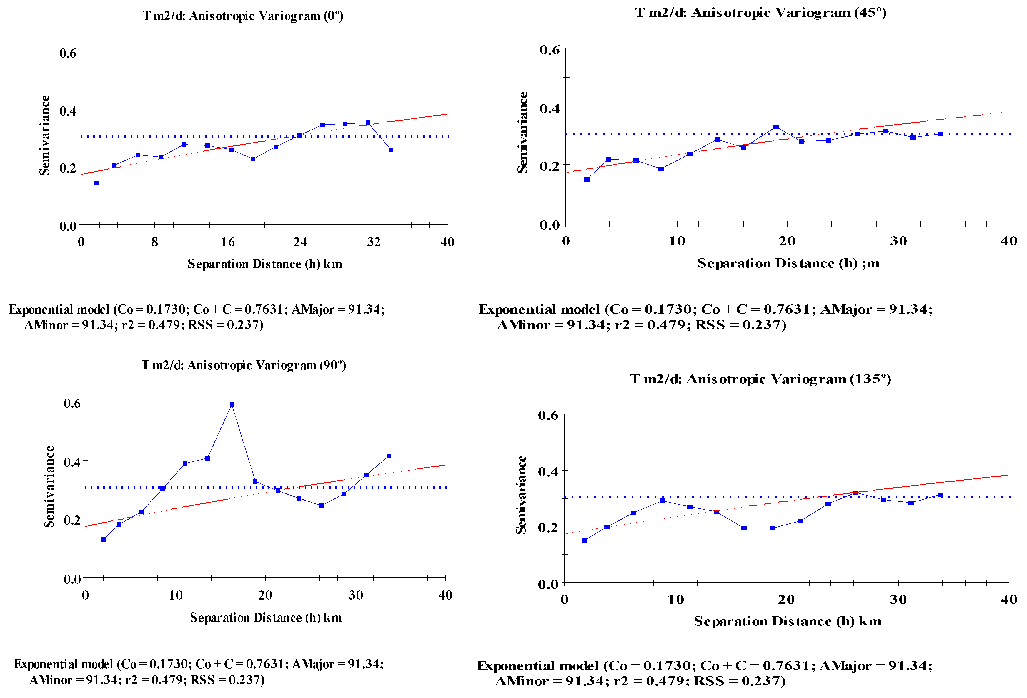
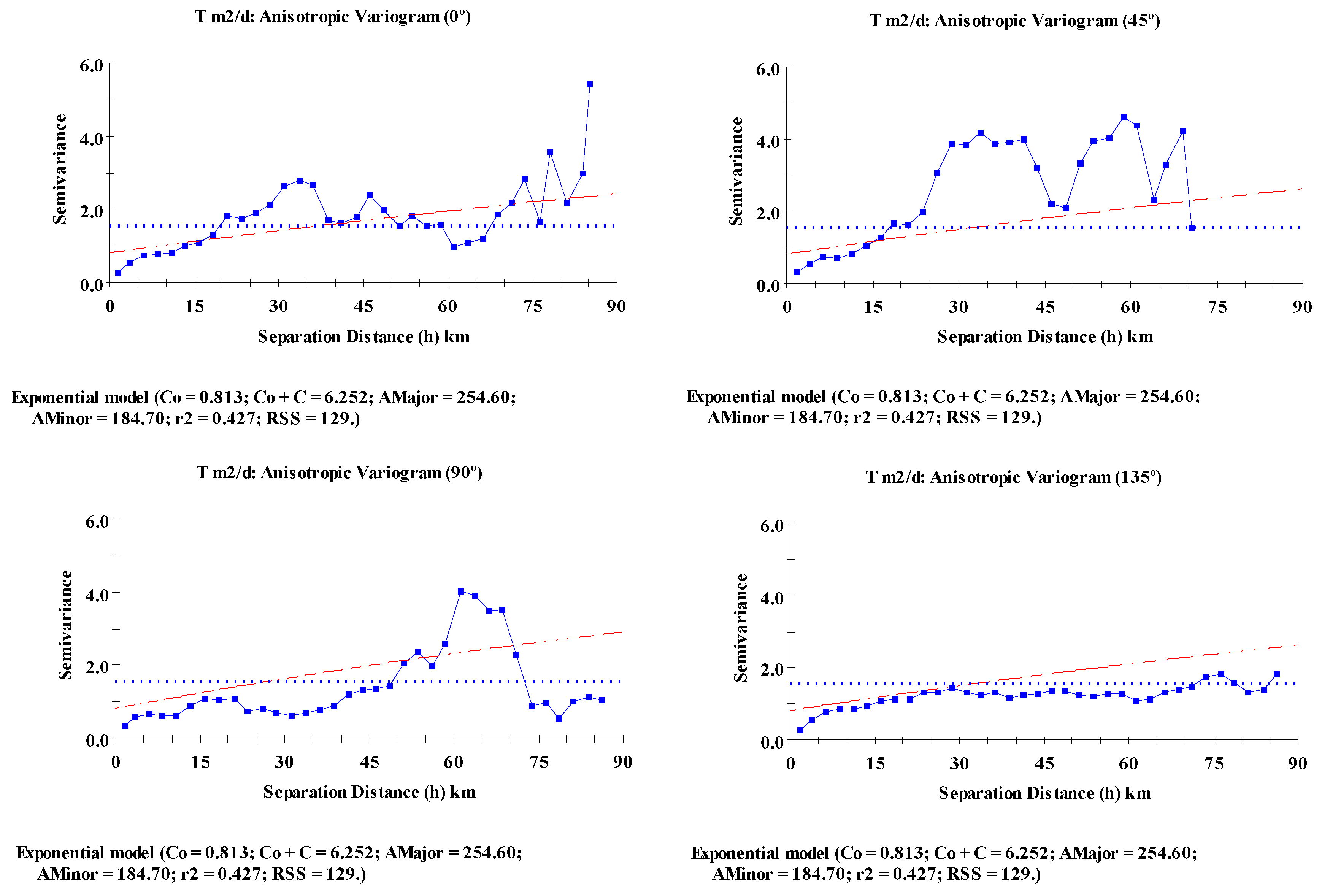
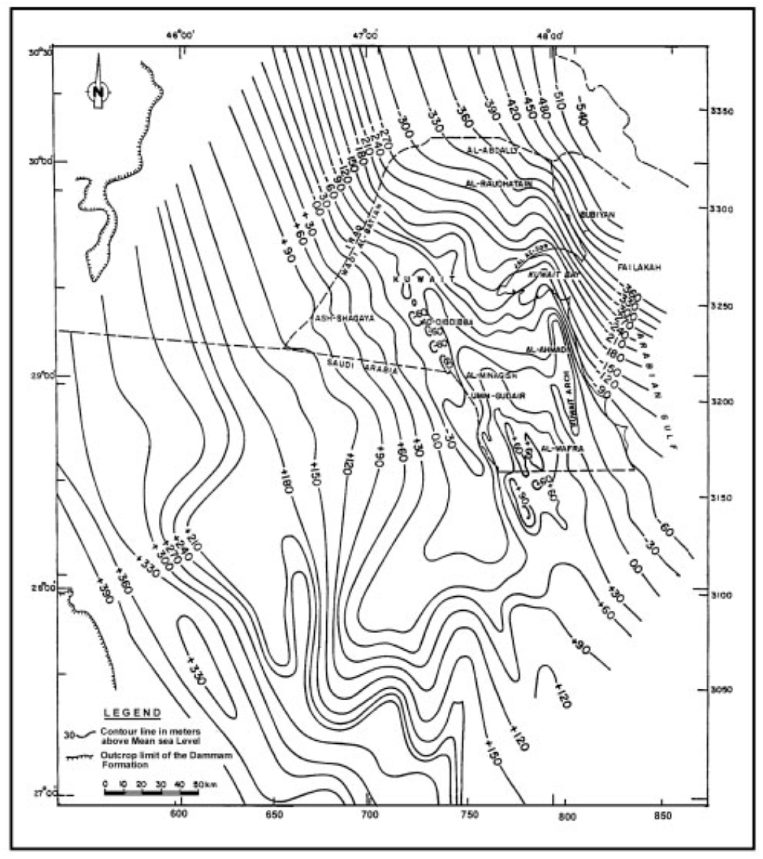
The directional semivariogram for four directional classes (0°, 45°, 90°, and 135°) was computed for both the Kg and Dm aquifers. There Kg aquifer shows anisotropy in T values in 90° (Figure 7). However, in Dm aquifer, a very clear anisotropy is evident (Figure 8), and there are distinct differences in the structure in all the four directions; the two directional variograms (representing 0° and 45°) rise more sharply than the other two directions (90° and 135°). This confirms the presumption of earlier workers that the Dm aquifer possesses highly anisotropic transmissivity due to karst networks [12]. Moreover, the dominantly observed orientation of the anisotropy becomes more significant when related to the structural geology of the Dammam Formation. The general trend of the major elongated anticline and synclinal structures in southern and central Kuwait (Figure 9) is in the north-northwest direction [30]. These structures are associated with major faulting, fracturing, shear zones as well as very small closure anticlines, running in the north-northeast direction [31,32]. This corresponds to the T from the directional variogram.
2.8. Transmissivity Kriging
Kriging is an effective interpolation technique that considers both distance and degree of variation between data points for estimating value at any unknown location [7,34]. The kriging weights were obtained by fitting semi-variogram models, in this study block ordinary kriging was used. The linear, Gaussian, spherical, and exponential models were tested with the lag distance to select the best fitting.
A block ordinary kriging using the 16 nearest neighbors within a radius of 167 and 170 km for Kg and Dm aquifer, respectively, was performed to estimate the transmissivity values at an unknown location in both Kg and Dm aquifers. The log(T) structural models, given by Equation (4), were used in the estimation of the transmissivity function distribution. Furthermore, the variance of the error of the estimate was obtained. The computation was carried out using the three-dimensional kriging module of the GS+ software, which uses the following kriging equations [18]:
where is the weighting function of each point, j, to be used in the estimation of point x0; γ(xi − xj) is the variogram value for the distance between xi and xj, and μ is the Lagrange multiplier. The variance of the error of estimation for point x0 is given as
2.9. Cross Validation
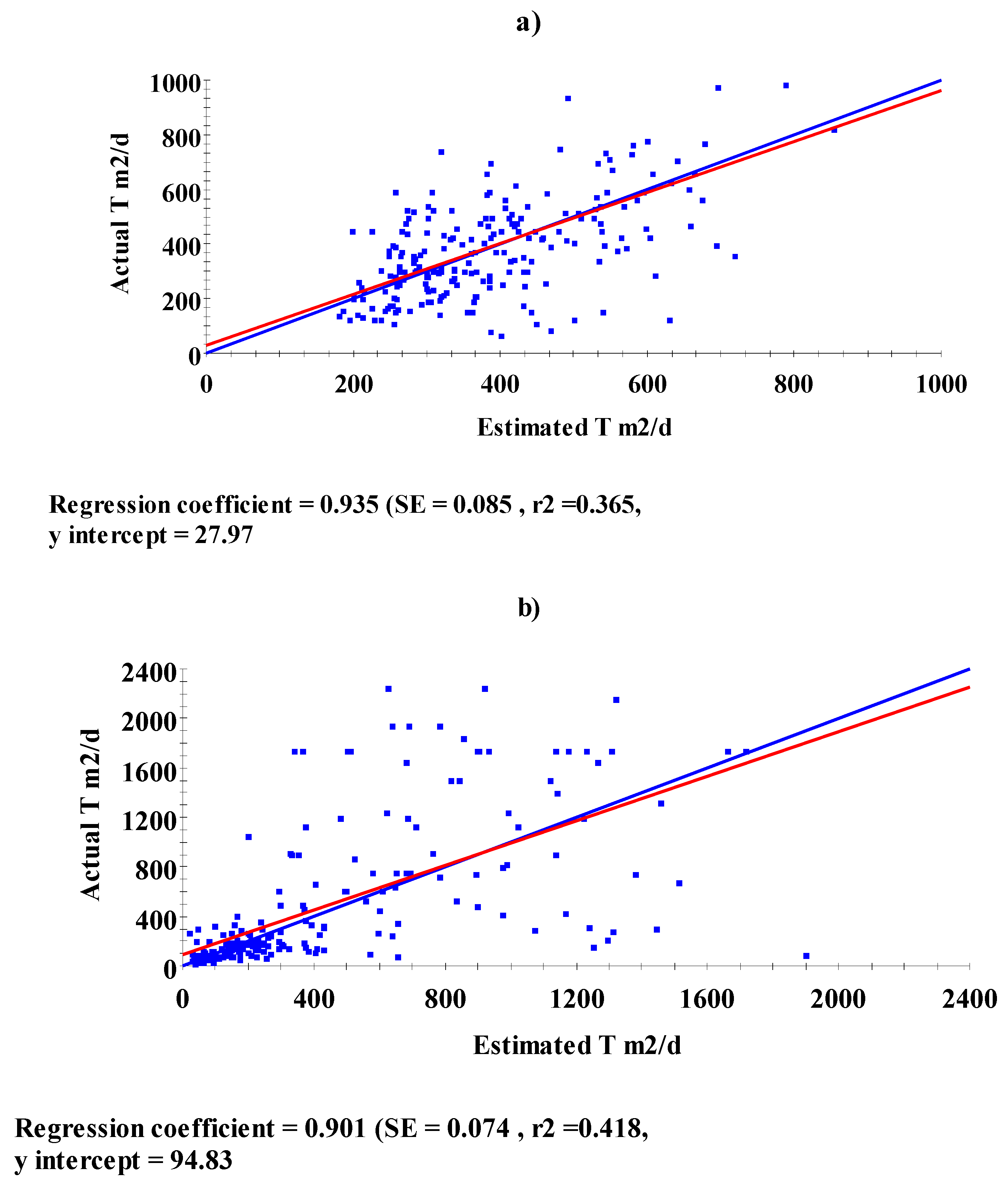
Cross validation was carried out to reexamine the fitted models by systematically changing the lag distance, uniform distance, and the model type. Four types of variogram models, including linear, Gaussian, spherical and exponential, were reexamined with different lag distance. Scatter plots of the true values versus the estimated values are illustrated in Figure 10a,b. These show regression coefficients of 0.935 and 0.901, for Kg and Dm aquifers, respectively.
The coefficient of the least squares model describes the linear regression equation between the actual and estimated values. The regression coefficient will be 1.0 for the best fit, shown by the blue line in Figure 10a,b. These values were the highest values obtained among the examined models and the lag distances. Accordingly, the exponential model was selected based on the criteria and the difference between the actual and estimated values (Table 3).
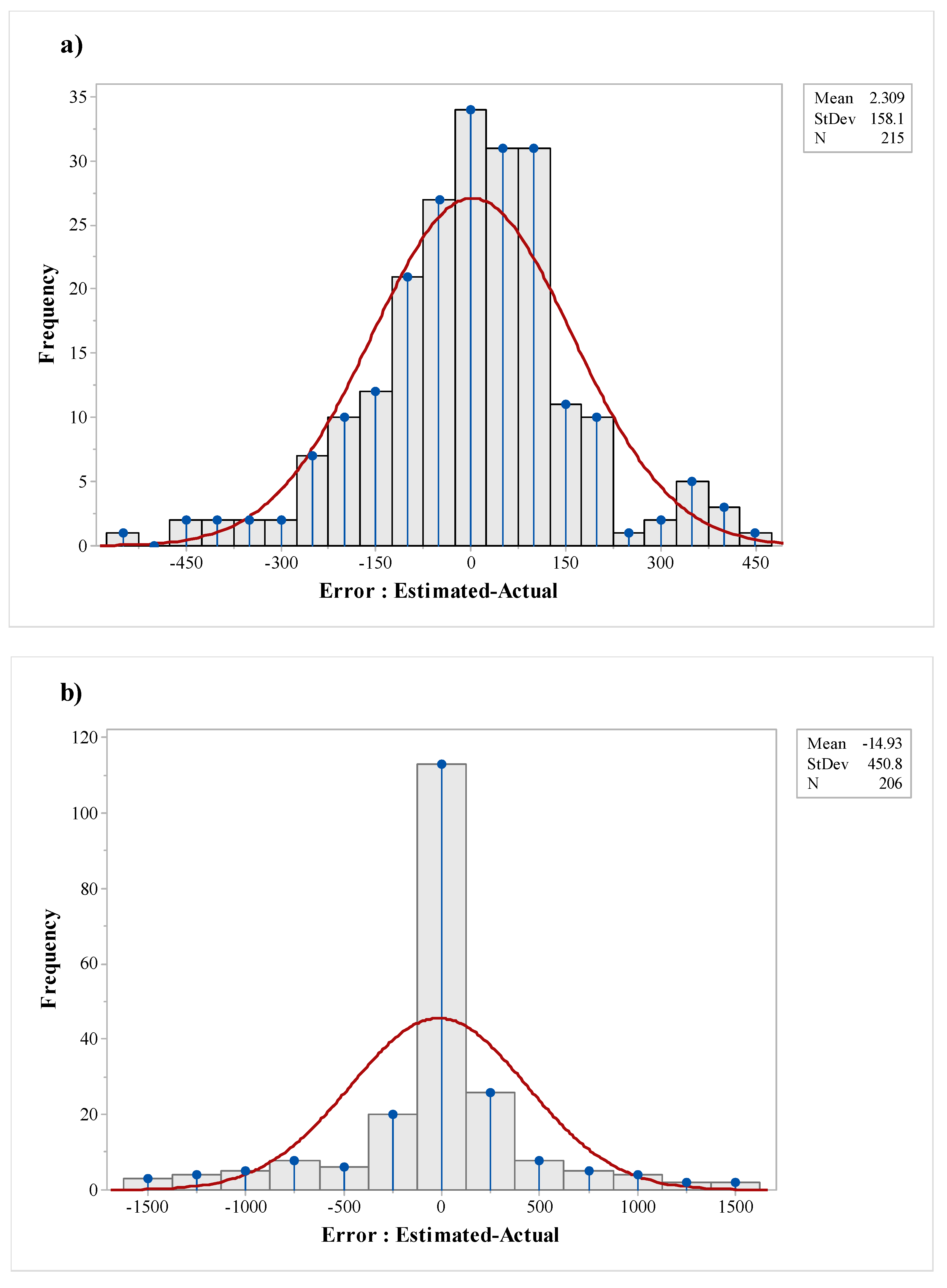
The r2 is low for both Kg (0.365) and Dm (0.418). It is worth mentioning that high r2 is certainly a yardstick for the fitness of the model, but not the sole criterion, especially for predictive purposes. The low root mean square error (RMSE) is of more practical usefulness in a predictive model [35]. A useful rule of thumb is that the test set RMSE should be less than 10% of the range of target property value. The RMSE was calculated for both the Kg and Dm aquifers (Figure 11 and Table 3). The mean of the error of Kg and Dm were 2.309 and −14.930, respectively. The means are not zero, although they are well within the 10% range of the target value.
The lower RMSE for Kg aquifer can be explained with a lesser variation in T values i.e., 61 to 1252 m2 d−1 compared to Dm aquifer, where the RMSE was −14.93 and the T value ranged from 22 to 2237 m2 d−1. This higher variation in T within Dm aquifer is due to karst development, and the fractures within the carbonate aquifer; field observations have also confirmed these inferences and frequent loss of circulation was observed in drilling reports. The T values for Dm aquifers are underestimated, but within very close range of the measured values. The r2 obtained after cross validation for the simulated values for Kg and Dm aquifers were 0.418 and 0.423, and they were within the range of 0.366 to 0.428 for the different active lag distances, class distance, and models, and the standard error prediction defined by relation SDx(1 − r2), where the SD = standard deviation of the actual data.
3. Results
A spatial map has been generated from the T values obtained by geostatistical techniques for Kg and Dm aquifers (Figure 12 and Figure 13). The transmissivity distribution map of Kg aquifer (Figure 12) indicates that the transmissivity of the aquifer increases from <50 m2 day−1 in the southwestern corner of Kuwait to about 400 m2 day−1 to the northeast, which appears to be following the general trend in the saturated thickness of the aquifer. This general trend is interrupted by several local anomalies where the aquifer has low transmissivity due to presence of a gatch layer. The low transmissivity anomalies (<50 m2 day−1) are attributed to the reduction of the aquifer-saturated thickness on top of the anticline structures (Figure 3). The high transmissivity anomalies (>700 m2 day−1) are attributed to the thickening of the saturated aquifer at the synclinal structure, and may be also due to the presence of extended faults from deeper strata.
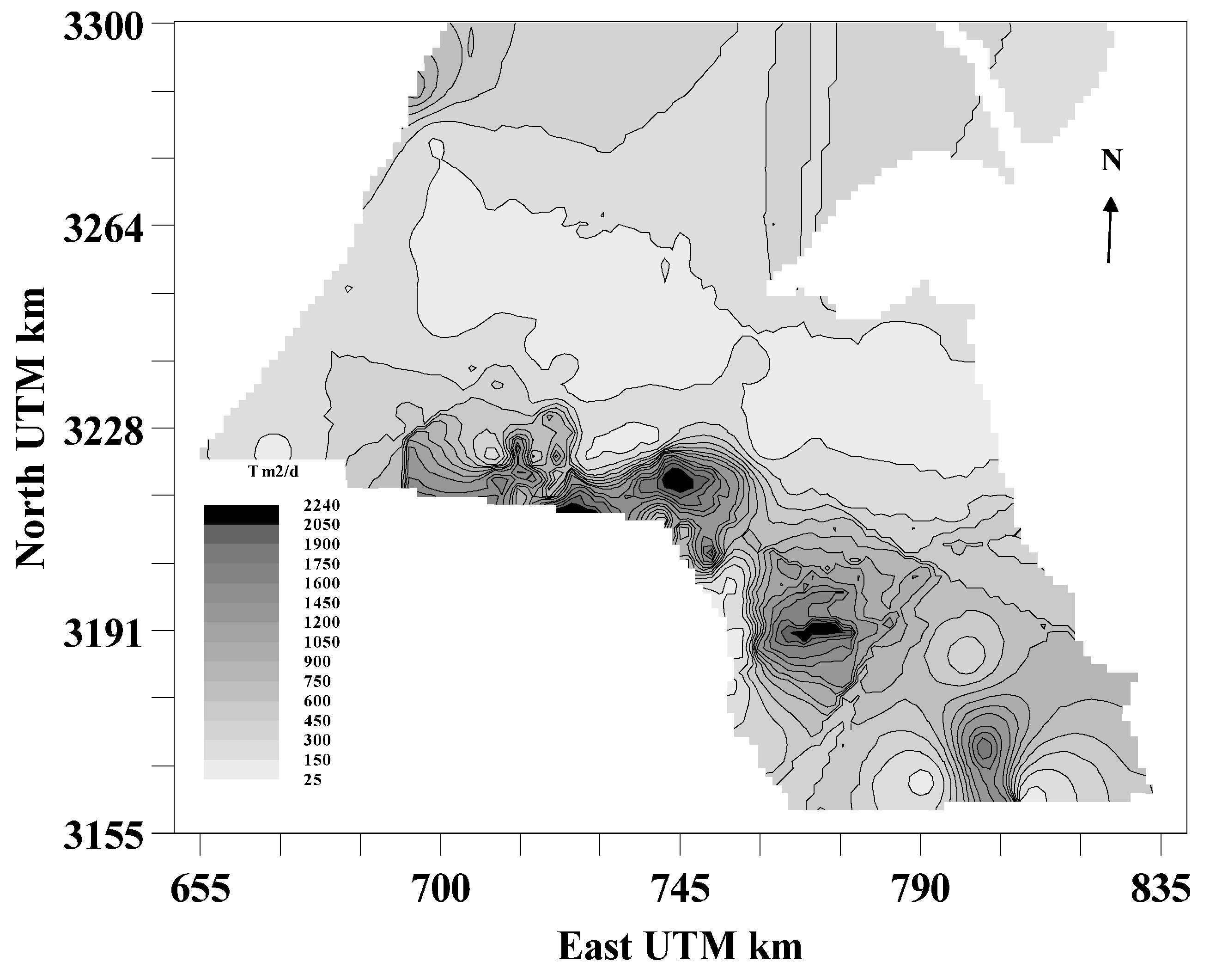
The spatial map for T of Dm aquifer depicts a ranges <100 m2 day−1 to ~2200 m2 day−1 (Figure 13). The high T values are located in the southern parts of Kuwait, and coincide with the areas of major anticline, lineations, and fault. Furthermore, these high transmissivity fields are located in the areas where the aquifer is recharged by fresher water from the southwest. On the other hand, low T fields are found to the north and northeast of these structures, and where the water in Dm aquifer is stagnant. This might be used to confirm that the Dm aquifer transmissivity is enhanced by preferential dissolution of the original rock matrix along weak planes (such as faults, joints, etc.), which are concentrated at the areas of anticlines.
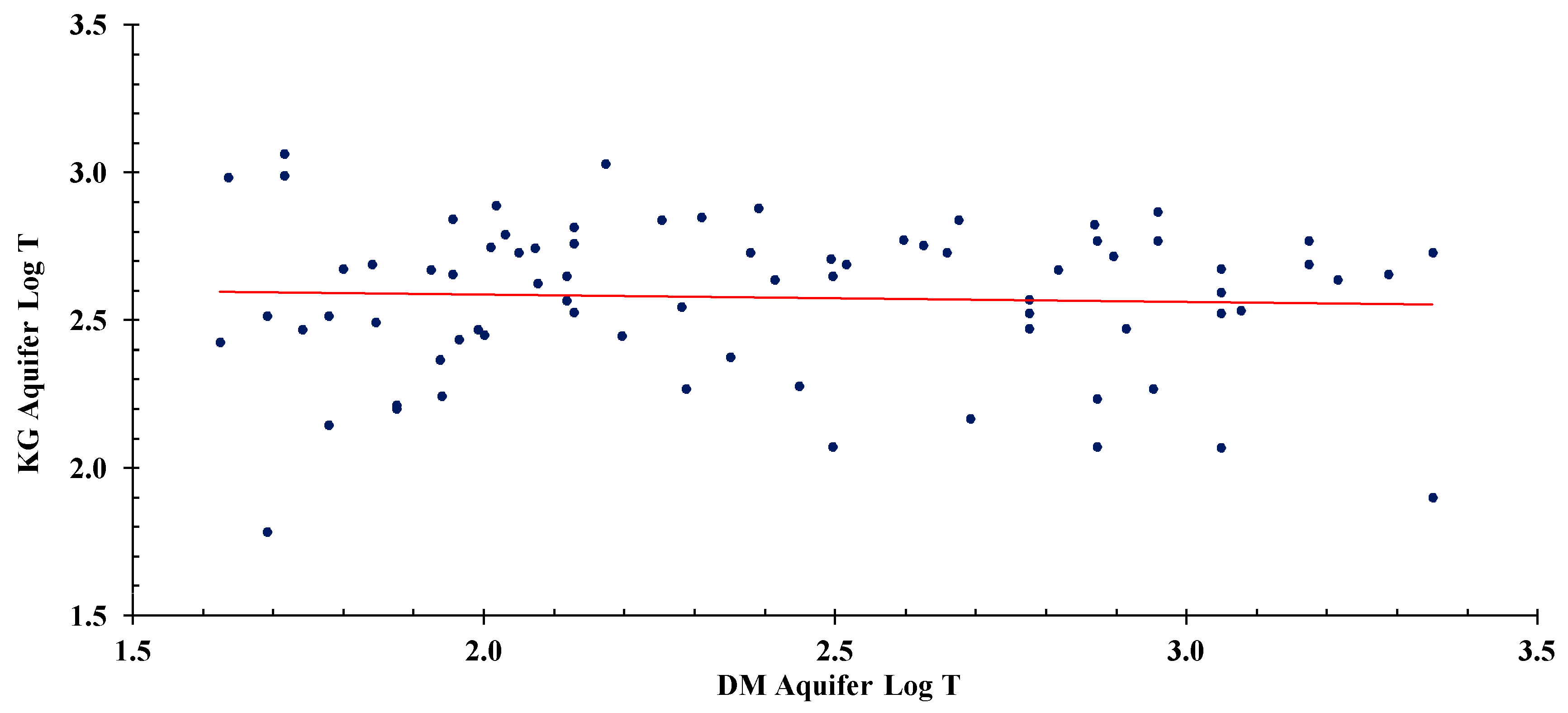
The spatial data coverage of Dm aquifer was much larger than Kg aquifer (Figure 3). The T obtained from kriging for the two aquifers has a certain degree of correlation. Co-kriging was the next logical step in this geostatistical analysis, with the aim that T of Kg aquifer could be better estimated using the widespread Dm aquifer T. There were 78 identical locations that were tested. The T values for these were not correlated, and the correlation coefficient was 0.047 (Figure 14). This is essentially due to the difference in intrinsic characteristics of the two aquifers compared.
4. Discussion
The applied geostatistical techniques are useful for extrapolating the T over large spatial domains. The use of kriging for T estimation proved to be valid both for Kg aquifer that contains sand, silt, and clay (essentially a variable lithology), and the Dm aquifer having nearly uniform limestone lithology. The use of geostatistical tools to derive T values correlate well with the measured values, and can reduce the uncertainty in wellfield development, and can complement the expensive well testing.
The T of the two aquifers is represented as a random spatial function where heterogeneity is described by the probability distribution and variogram of sample values. A structural analysis was performed which consisted of the construction and interpretation of sample variograms and the selection of model variograms to best fit the structure of the log-transformed transmissivity. The analysis indicated that the Dm aquifer is highly anisotropic, and has a longer range of influence and more substantial variance (39 km, 333,487) than the Kg aquifer (10 km, 44,613).
The model variograms were used in the kriging analysis to estimate the spatial average value of the T for the two aquifers in Kuwait. The estimated transmissivity distribution in the two aquifers was validated by geological and hydrological data. The estimated Dm aquifer T ranges from about 100 to 2200 m2/day, with high transmissivity fields coinciding with both the areas of major anticline and fault structures, and the areas of aquifer recharge by fresh water. Low T fields are located in the areas where the aquifer waters are stagnant. The estimated T for Kg aquifer ranges from <50 to about 800 m2 day−1, and is controlled principally by the saturated thickness of the aquifer.
The performed structural analysis and the estimated transmissivity and their associated variance fields for the two aquifers can be a critical input for developing a groundwater model that can aid in sustainable development and management of the wellfields in Kuwait.
The exponential model and lag distance are useful to estimate T values in a similar geological setting, both in isotropic and anisotropic formations. The extrapolated T values using kriging can be used for development of numerical modeling studies (deterministic and stochastic) for the aquifer system in the region. The T values can be used effectively in defining artificial recharge or underground water storage areas in the aquifers and in optimizing placement of future wellfield developments.
Author Contributions
M.A.-M. conceived the idea and carried out substantial part of the write-up. He was also leading the geostatistical work. W.K.Z. was involved in geostatistical modeling work. S.U. participated in the write-up of the manuscript.
Acknowledgments
The authors would like to thank the Ministry of Electricity and Water, Kuwait for providing aquifers transmissivity data, geological and hydrological maps. Thanks are due to Kuwait Institute for Scientific Research for supporting the research.
Conflicts of Interest
The authors declare no conflict of interest. All the data reported is exactly reported without any influence from any organization.
References
- Krâsny, J. Tranasmissivity and permeability distribution in hard rock environment: A regional approach. In Proceedings on Hard Rock Hydrosystems, S2 at Rabat, IAHS Publication; IAHS: London, UK, 1997; Volume 241, pp. 81–90. [Google Scholar]
- Marsily, G.D.; Delay, F.; Goncalves, J.; Renard, P.; Teles, V.; Violette, S. Dealing with spatial heterogeneity. Hydrogeology 2005, 13, 161–183. [Google Scholar] [CrossRef] [Green Version]
- Mace, R.E.; Smyth, R.C.; Xu, L.; Liang, J. Transmissivity, hydraulic conductivity, and storativity of the Carrizo-Wilcox Aquifer in Texas. In The University of Texas at Austin Bureau of Economic Geology Final Report Submitted to the Texas Water Development Report; BEG: Austin, TX, USA, 2000. [Google Scholar]
- Isaaks, E.H.; Srivastava, R.M. Applied Geostatistics; Oxford University Press Inc.: New York, NY, USA, 1989. [Google Scholar]
- Delhomme, J.P. Kriging in the hydrosciences. Adv. Water Resources, 1. Adv. Water Resour. 1978, 1, 251–266. [Google Scholar] [CrossRef]
- Crosbie, R.S.; Peeters, L.J.M.; Herron, N.; McVicar, T.R.; Herr, A. Estimating groundwater recharge and its associated uncertainty: Use of regression kriging and the chloride mass balance method. J. Hydrol. 2017. [Google Scholar] [CrossRef]
- Sahoo, S.; Jha, M.K. Analysis of spatial variation of groundwater depths using geostatistical modeling. Int. J. Appl. Eng. Res. 2014, 9, 317–322. [Google Scholar]
- Uddin, S.; Al-Ghadban, A.N.; Al Khabbaz, A. Localized Hyper Saline Waters in Arabian Gulf from Desalination activity—An example from South Kuwait. Environ. Monit. Assess. 2010, 181, 587–594. [Google Scholar] [CrossRef] [PubMed]
- Mukhopadhyay, A.; Akber, A.; Al-Awadi, E.; Burney, N. Analysis of Freshwater Consumption Pattern in Kuwait and its Implications for Water Management. Water Resour. Dev. 2000, 16, 543–561. [Google Scholar] [CrossRef]
- Mukhopadhyay, A.; Al-Otaibi, M. Development, Analysis and Integration of Hydrological Data in Kuwait (WM010C) Volume 2: Hydrological Maps of Kuwait; Report No. KISR7434; Kuwait Institute for Scientific Research: Kuwait City, Kuwait, 2005. [Google Scholar]
- Sakr, I.M. An Introduction to Groundwater in the Gulf Cooperation Council Countries; Al-Ain Advertising, Publishing, and Distribution Co.: Al-Ain, United Arab Emirates, 1988. (In Arabic) [Google Scholar]
- Burdon, D.J.; Al Sharhan, A. The problem of the paleokarstic Dammam Limestone Aquifer in Kuwait. J. Hydrol. 1968, 6, 358–404. [Google Scholar] [CrossRef]
- Omar, S.A.S.; Misak, R.; King, P.; Shahid, S.A.; Abo-Rizq, H.; Grealish, G.; Roy, W. Mapping the vegetation of Kuwait through reconnaissance soil survey. J. Arid Environ. 2001, 48, 341–355. [Google Scholar] [CrossRef]
- Corporation, P. Groundwater Resources in Kuwait; Ministry of Electricity and Water, State of Kuwait: Kuwait City, Kuwait, 1963; Unpublished Report. [Google Scholar]
- Amer, A.; Barrat, J.M.; Mukhopadhyay, A. Assessment of groundwater resources in Kuwait using a finite difference model. Water Resour. Dev. 1990, 6, 104–114. [Google Scholar] [CrossRef]
- Uddin, S.; Al Dosari, A.; Al Ghadban, A.N.; Aritoshi, M. Use of interferometric techniques for detecting subsidence in the oil fields of Kuwait using Synthetic Aperture Radar Data. J. Pet. Sci. Eng. 2006, 50, 1–10. [Google Scholar] [CrossRef]
- Woodbury, A.; Sudicky, E.A. The geostatistical characteristics of the Borden aquifer. Water Resour. Res. 1991, 27, 533–546. [Google Scholar] [CrossRef]
- Marsily, G.D. Quantitative Hydrogeology; Academic Press: San Diego, CA, USA, 1986. [Google Scholar]
- Delhomme, J.P. Spatial variability and uncertainty in groundwater flow parameters: A geostatistical approach. Water Resour. Res. 1979, 15, 269–280. [Google Scholar] [CrossRef]
- Freeze, R.A. A stochastic-conceptual analysis of one-dimensional groundwater flow in non-uniform homogeneous media. Water Resour. Res. 1975, 11, 725–742. [Google Scholar] [CrossRef]
- Neuman, S.P. Statistical characterization of aquifer heterogeneities: An overview, in recent trends in hydrogeology. Geol. Soc. Am. 1982, 189, 81–102. [Google Scholar]
- Matheron, G. The Theory of Regionalized Variables and Its Applications; Report No. 5; CGMM: Ecole des Mines: Fontainebleau, France, 1971. [Google Scholar]
- Shafer, J.M.; Varljen, M.D. Approximation of confidence limits on sample semivariograms from single realizations of spatially correlated random fields. Water Resour. Res. 1990, 26, 1787–1802. [Google Scholar] [CrossRef]
- Matheron, G. Principles of geostatistics. Econ. Geol. 1963, 58, 1246–1266. [Google Scholar] [CrossRef]
- Cressie, N.; Hawkins, D.M. Robust estimation of the variogram: I. J. Int. Associ. Math. Geol. 1980, 12, 115–125. [Google Scholar] [CrossRef]
- Dowd, P.A. The variogram and kriging: Robust and resistant estimators. Geostatisticsfor Natural Resources Characterisation. In Series C: Mathematical and Physical Sciences; Verly, G., David, M., Journel, A.G., Marechal, A., Eds.; Reidel Publishing Company: Dordrecht, The Netherlands, 1984; Volume 122, pp. 91–106. [Google Scholar]
- Omre, H. The Variogram and its Estimation. In Geostatistics for Natural Resources Characterization: Part 1; Verly, G., David, M., Journel, A.G., Marechal, A., Eds.; Springer: Dordrecht, The Netherlands, 1984; pp. 107–125. [Google Scholar]
- Istok, J.D.; Cooper, R.M.; Flint, A.L. Three dimensional cross-semivariogram calculation for hydrogeological data. Groundwater 1988, 26, 638–646. [Google Scholar]
- Henley, S. Non-Parametric Geostatistics; Springer: Dordrecht, The Netherlands, 1981. [Google Scholar]
- Salman, A.M. Geology of the Jal Az-Zor, Al-Liyah Area. Master’s Thesis, Geology Department, Kuwait University, Kuwait City, Kuwait, 1979. [Google Scholar]
- Geophysique, C.G.D. Shagaya Geophysical Survey; Ministry of Electricity and Water, State of Kuwait: Kuwait City, Kuwait, 1968; Unpublished Report. [Google Scholar]
- Al-Sarawi, M. Tertiary faulting beneath Wadi Al-Batin (Kuwait). Geol. Soc. Am. Bull. 1978, 91, 610–618. [Google Scholar] [CrossRef]
- Al-Sulaimi, J.; Al-Rabba, S.; Al-Muhanna, A.; Amer, A.; Lenindre, Y. Assessment of Groundwater Resources in Kuwait Using Remote Sensing Technology; Report Kuwait Institute for Scientific Research; KISR: Fort Smith, AR, USA, 1992. [Google Scholar]
- Goovaerts, P. Geostatistics for Natural Resources Evaluation; Oxford University Press: New York, NY, USA, 1997. [Google Scholar]
- Alexander, D.L.J.; Tropsha, A.; Winkler, D.A. Beware of R(2): Simple, unambiguous assessment of the prediction accuracy of QSAR and QSPR models. J. Chem. Inf. Model. 2015, 55, 1316–1322. [Google Scholar] [CrossRef] [PubMed]
Figure 1.
Location of the state of Kuwait and established groundwater wellfields (Source [10]).
Figure 1.
Location of the state of Kuwait and established groundwater wellfields (Source [10]).

Figure 2.
Generalized hydrostratigraphy of the Tertiary deposits in Kuwait and surrounding areas (Source: [16]).
Figure 2.
Generalized hydrostratigraphy of the Tertiary deposits in Kuwait and surrounding areas (Source: [16]).

Figure 3.
Surface elevation map of the Kuwait Group (Kg) aquifer and spatial location of the transmissivity (T) values for Dammam (Dm) (magenta) and Kg (dark blue) aquifers.
Figure 3.
Surface elevation map of the Kuwait Group (Kg) aquifer and spatial location of the transmissivity (T) values for Dammam (Dm) (magenta) and Kg (dark blue) aquifers.

Figure 4.
Histogram plots of the transmissivity of the Kg (a) and Dm (b) aquifers.

Figure 5.
Histogram of the log (T) of the Kg (a) and Dm (b) and percentage cumulative frequency of Kg (c) and Dm (d) aquifers.
Figure 5.
Histogram of the log (T) of the Kg (a) and Dm (b) and percentage cumulative frequency of Kg (c) and Dm (d) aquifers.

Figure 6.
Variograms of log(T) values of the Kg (a) and Dm (b) aquifers.

Figure 7.
Directional variograms of the log(T) of the Kg aquifer.

Figure 8.
Directional variograms of the log(T) of the Dm aquifer.

Figure 9.
Structural contour map of the top Dammam Formation in and around Kuwait (Source [33]).
Figure 9.
Structural contour map of the top Dammam Formation in and around Kuwait (Source [33]).

Figure 10.
Scatter plot of the estimated versus the actual T values of Kg (a) and Dm (b) aquifer.

Figure 11.
Histogram of the error estimation of Kg (a) and Dm (b) aquifer.

Figure 12.
Estimated transmissivity distribution of the Kg aquifer.

Figure 13.
Estimated transmissivity distribution of the Dm aquifer.

Figure 14.
Regression analysis between Kg log T and Dm log T values.


Table 1.
Summary statistics for the transmissivity of the Dm and Kg aquifers in Kuwait.
| Parameters | Kg Aquifer | Dm Aquifer |
|---|---|---|
| N | 216 | 206 |
| Mean | 393.88 | 478.62 |
| Variance | 44,612.92 | 333,487.05 |
| Standard Deviation | 211.22 | 577.48 |
| Minimum Value | 61.00 | 22.0 |
| Maximum Value | 1252.00 | 2237 |
| Skewness(se) | 1.23 (0.17) | 1.46(0.17) |
| Kurtosis (se) | 2.16 (0.33) | 0.90(0.34) |
Table 2.
Fitted parameters for model semivariogram.
| Parameters | Log(T) | |
|---|---|---|
| Kg Aquifer | Dm Aquifer | |
| Active lag distance km | 35.0 | 87.0 |
| Class distance Interval km | 2.5 | 2.5 |
| No. of classes | 14 | 39.0 |
| Minimum pairs | 372 | 169 |
| Maximum pairs | 1315 | 1090 |
| Fitted Model | Exponential | Exponential |
| Nugget variance (C0) | 0.018 | 0.004 |
| Sill (C + C0) | 0.291 | 1.799 |
| Range (a) km | 10.53 | 39.0 |
| SRR | 7.078 × 10⁻³ | 1.49 |
| r2 | 0.785 | 0.797 |
| Proportion C/(C0 + C) | 0.939 | 0.998 |
Table 3.
Cross validation results of Kg and Dm aquifers.
| Parameters | Log(T) | |
|---|---|---|
| Kg Aquifer | Dm Aquifer | |
| Regression Coefficient | 0.920 | 0.784 |
| Standard Error | 0.074 | 0.064 |
| r2 | 0.418 | 0.423 |
| Mean squared error | 2.619 | −14.928 |
© 2018 by the authors. Licensee MDPI, Basel, Switzerland. This article is an open access article distributed under the terms and conditions of the Creative Commons Attribution (CC BY) license (http://creativecommons.org/licenses/by/4.0/).
Share and Cite
MDPI and ACS Style
Al-Murad, M.; Zubari, W.K.; Uddin, S. Geostatistical Characterization of the Transmissivity: An Example of Kuwait Aquifers. Water 2018, 10, 828. https://doi.org/10.3390/w10070828
AMA Style
Al-Murad M, Zubari WK, Uddin S. Geostatistical Characterization of the Transmissivity: An Example of Kuwait Aquifers. Water. 2018; 10(7):828. https://doi.org/10.3390/w10070828
Chicago/Turabian StyleAl-Murad, Mohammad, Waleed K. Zubari, and Saif Uddin. 2018. "Geostatistical Characterization of the Transmissivity: An Example of Kuwait Aquifers" Water 10, no. 7: 828. https://doi.org/10.3390/w10070828
Note that from the first issue of 2016, this journal uses article numbers instead of page numbers. See further details here.