Functional Relationship between Soil Slurry Transfer and Deposition in Urban Sewer Conduits


1
Department of Civil and Environmental Engineering, Hanbat National University, Daejeon 34158, Korea
2
Research Center for Disaster Prevention Science and Technology, Korea University, Seoul 02841, Korea
*
Author to whom correspondence should be addressed.
Water 2018, 10(7), 825; https://doi.org/10.3390/w10070825
Submission received: 5 May 2018
/
Revised: 20 June 2018
/
Accepted: 21 June 2018
/
Published: 22 June 2018
(This article belongs to the Special Issue Modeling and Practice of Erosion and Sediment Transport under Change)
Abstract
:Soil slurry deposited on the surface of the Earth during rainfall mixes with fluids and flows into urban sewer conduits. Turbulent energy and energy dissipation in the conduits lead to separation, and sedimentation at the bottom lowers the discharge capacity of conduits. This study proposes a functional relationship between shear stress in urban sewer conduits and the physical properties of particles in a conduit bed containing less than 20 mm of soil. Several conditions were implemented for analyzing two-phase flow (soil slurry and fluid in urban sewer conduits) in terms of turbulent flow by considering soil slurry flowing into urban sewer conduits. The internal flows of fluid and soil slurry in urban sewer conduits were numerically analyzed and modeled by applying the Navier–Stokes equation and the k- turbulence model. The transfer deposition of the soil slurry in the conduits was reviewed and, based on the results, a limiting tractive force was calculated and used to propose criteria for transfer deposition occurring in urban sewer conduits.
1. Introduction
It is important to understand the flow characteristics of urban sewer conduits to maintain their flow control capacity and prevent flooding during rainfall. In the case of localized and heavy rainfall, soil slurry separates from the Earth’s surface through outflows and flows into drainage. This lowers the discharge capacity of drains. Delaying the outflow leads to overflow that causes flooding. Under a balanced condition, sediments accumulated at the bottom of urban sewer conduits are directly related to a reduction in discharge capacity, and leads to system overload and flooding.
The purpose of urban sewer conduits is to prevent flooding in urban areas by discharging runoff generated during rainfall. Together with the design and construction of such urban sewer conduits, maintaining their discharge capacity is the most important factor influencing continual maintenance. If urban sewer conduits are not designed, constructed, and maintained properly, severe soil sedimentation can occur in them during or after rainfall events, which threatens their discharge capacity and ability to properly handle sediments. Reduced discharge capacity of urban sewer conduits can cause flooding during the rainy season or localized heavy rainfalls.
In general, soil slurry flowing into urban sewer conduits forms a layer of solid particles at the bottom of the conduit leading to deposition [1,2,3,4]. In terms of flow characteristics, when particles are transferred, the fluid and solid particles interact in a complex manner. Past research has relied on experiments [5], but it is challenging in experimental analyses to review the independent influence of each variable on transfer deposition. Moreover, soil slurry has a dynamic flow in the transfer process. In the case of particles, it is difficult to measure the internal flow velocity of a conduit because of their own viscosities, particle sizes, and fluid drag forces [6,7]. Using experimental results, many studies have analyzed the fundamental aspects of sediment transfer in turbulent flow conditions [8]. However, they propose representing sediment flow as an induction equation to relate it to flow velocity [9,10,11,12]. Knowledge of the characteristics of internal flow is critical. However, the internal flow of urban sewer conduits is completely different from that of a river, making it difficult to obtain accurate predictions. For this purpose, existing empirical equations based on flow along a river may be applicable if modified according to the hydraulic features of urban sewer conduits.
It is difficult to determine the initiation of particle movement because of various issues. The Shields diagram is a typical criterion for the incipient motion of sediments [13]. Shields suggested fundamental concepts for initiating the motion of a bed comprising non-cohesive particles resistant to erosion by flowing water. This is indicated by critical shear stress, which is commonly assumed to be a constant for a given sediment mixture and can be determined through laboratory experiments [14]. However, the proposed results cannot be directly applied owing to some limitations. Shields did not provide any method to obtain critical shear stress for transfer and deposition. Accordingly, Brownlie fitted a curve to the representative line using the Shields relationship [15]. In this study, the precise moment of incipient motion is suggested, mainly based on numerical modeling, and transport rate measurements are used for a more objective evaluation of the various conditions of the deposition environment.
To efficiently model the transfer deposition of soil in a conduit, it is necessary to determine the shear stress to smoothly model the transfer of particles without deposition in the conduit. To review the characteristics of the transfer deposition of particles in turbulent flow, some studies have applied obstacles in pipes or conduits, attended to the flow of particles in the relevant region, and applied the results to various technologies [16,17,18]. Some of these studies focused on one phase of the fluid to analyze the mechanism of its continuity and momentum equations, and applied the advection–diffusion equation to the soil slurry sediment. However, such methods are limited to the analysis of particle deposition and sedimentation.
Studies based on numerical analysis to reflect the conditions of turbulent flow have modeled the transfer deposition of soil and correlations among multiple parameters. The results have been compared with those of the above-mentioned empirical equation to suggest a proper method of application [19,20,21,22].
This study proposes a functional relationship between critical tractive force in urban sewer conduits and the physical properties of particles in a conduit bed containing less than 20 mm of soil. The inlet flow velocity (1.0, 2.0 and 3.0 m/s) of the soil slurry mixture, the volume concentration of the soil (10%, 30% and 50%), and its particle size were set as variables. Soil slurry flowing into urban sewer conduits was analyzed based on the two-phase flow (soil slurry and fluid in urban sewer conduits) as turbulent flow. In a relevant work, Song et al. studied the flow of soil slurry in urban sewer conduits [23]. In reviewing flow, the shear flow velocity and shear stress were found to be critical. Therefore, the results of Song et al. were applied in this study. The purpose was to review the criteria of deposition in the transfer process by assuming that soil slurry can flow in urban sewer conduits and by changing its flow conditions. It is noteworthy that the observation and analysis of the two-phase flow are difficult, and no relevant study has considered this for soil slurry. This study made the following assumptions:
- The flow of a mixture of fluid and soil slurry in urban sewer conduits was considered, similar to simulating the mixing and flowing of a large amount of soil slurry and runoff.
- In conditions of turbulent flow, it was assumed that flow in the conduit consisted of fluid and solid phases.
- For accurate flow analysis, incidental simulations were excluded, and a method for reducing the time needed to analyze a short conduit was considered.
- Soil flowing in a sewer conduit consists of particles of different sizes. For modeling, it is necessary to consider this distribution of particle size. In this study, it was assumed that the soil slurry had a uniform particle size distribution.
A commercial analysis tool ANSYS FLUENT 13.0 was used in this study [24]. This study analyzed the characteristics of flow in urban sewer conduits of 10 m length and 0.6 m diameter in light of the inlet flow velocity of the soil–fluid mixture (v), size of the soil particle (d), and the volume fraction in the soil mixture (v/f). The simulation results were used to investigate the limiting tractive force. Based on the results of a hydrodynamic analysis using 2D modeling, the limiting tractive force was calculated depending on the particle size of the soil slurry, and an equation for the functional relationship based on a different particle size was proposed. The limiting tractive force was found to be related to the physical properties of non-cohesive soil.
2. Numerical Method
In past studies on two-phase flow, the sensitivity of each phase was analyzed to propose the mechanism of their interaction [25,26,27,28]. These results provided a considerable amount of information concerning two-phase flow that was used to define the phenomenon for a variety of flows using a diversity of numerical analysis models. A few recent studies have proposed a functional equation based on particle density to define the criteria for sediment movement based on the flow velocity distribution of urban sewer conduits, in the context of two-phase flow containing a mixture of fluid and soil slurry [29,30,31].
2.1. Governing Equations and Mathematical Model
In this study, the models were constructed in FLUENT 13.0 to analyze two-phase flow using the ANSYS solver [32]. The control equations consisted of continuity and momentum equations and particle component conservation equations of mass and momentum [33]. The continuity and momentum equations can be implemented using Reynolds’ transport theorem, and by applying Newton’s second law [34,35].
The continuity equations are shown as Equation (1) and compressible fluid is presented as Equation (2). In Equation (3), the equations of momentum yield the volume fraction and density per unit time for each phase based on velocity. In the equation, represents the orthogonal coordinates, the orthogonal (directional) element of the velocity vector that represents average flow velocity, is fluid density, is pressure, and is the sum of influential forces, such as gravity, deflecting force, and centrifugal force.
In Equation (4), represents a viscous stress tensor representing Newtonian flow fluid, including the velocity of the deformed stress tensor; and represents structural correlation. In Equation (5), represents the ratio of the strain (deformation) tensor described in Equation (4):
2.2. Turbulence Model
To analyze the effect of turbulence in a conduit with soil slurry, a turbulence model is required. The shear force owing to the laminar viscous force of the neighboring fluid becomes its driving force and, consequently, a laminar flow with a certain layer appears. However, if the shear stress increases with increasing flow velocity, viscous force transmission becomes challenging to maintain. As a result, the shear stress breaks into very small turbulent eddies and ends up being transmitted inside the fluid.
In general, the Reynolds stress-based model is used to simulate turbulent flow [36,37,38,39]. To analyze turbulent flow, the authors used Launder and Spalding’s standard k-ε model, the universally used turbulence model [40]. In the model used to calculate the Reynolds factors, two equations representing the turbulent kinetic energy and the rate of dissipation of energy were calculated to represent turbulent viscosity. It is well known that the prediction of rotational flow or vortex flow, generated when particles of the fluid rotate about a certain axis, and the analysis of an area near a wall with a low Reynolds’ number is inaccurate. However, the model is excellent at convergence in basic turbulent analysis and shortening calculation time [32].
To analyze fluid flow in the standard k-ε model, two equations of turbulent energy and dissipation rate as well as a general transfer equation should be applied separately. These equations are called the turbulent kinetic energy equation and the turbulent kinetic energy dissipation equation, respectively, and are used as a two-equation model. is a model constant, which is generally 0.09. In this study, based on Equations (6) and (7) in the analysis of the transfer deposition of soil in a tube, k and ε are calculated in two separate transport equations (k-equation and ε-equation) to model turbulent stress [32].
In Equation (8), reflects the influence of viscous force, and each value represents the coefficient of the standard values of k and ε, which are obtained through experiments in a wide range of the turbulent area as proposed by Versteeg and Malalasekera (Table 1) [41]. The parameters presented in Table 1 were used to predict the shear flow of basic turbulence, including homogeneous and heterogeneous flows, and yield highly reliable results in terms of the boundary of the wall and free shear flow. , , and are empirical constants determined through experiments, and and are turbulent Prandtl numbers for turbulent kinetic energy and the rate of energy dissipation, respectively [42].
Data collected through experimental research on turbulent energy and the rate of dissipation were first applied as parameters in the model. Nevertheless, as this study focuses on analyzing phenomena based on modeling, the reliability of the parameters to be applied were not validated, and experimentally acquired values proposed in a manual were applied because the range of each parameter and ground for its application were required [32].
2.3. Setup and Boundary Conditions
In this study, the inlet, outlet, side wall, and symmetry of the entire conduit (volume) were defined as boundary conditions to consider the flow of particles and soil slurry in urban sewer conduits. The authors used ANSYS-FLUENT 13.0 for the analysis. In repeated numerical calculations, the relative error of a numerical solution was made to converge to 0.001. The relative error of the schemes is computed by comparing the result of the integration step. Reduce step size by half refine the step such that the change of outcome can be identified [24]. It took 17 h on average on an Intel(R) Xeon(R) CPU E5-2630, 2.40 GHz, with 16 GB RAM. The boundary conditions of the numerical model in this study are presented in Table 2.
It was assumed that the flow conditions did not change, and no deformed flow occurred. The authors simulated phenomena by analyzing various runoff flows in the conduit. This method helped reduce calculation time and implement an optimal solution through repeated calculations.
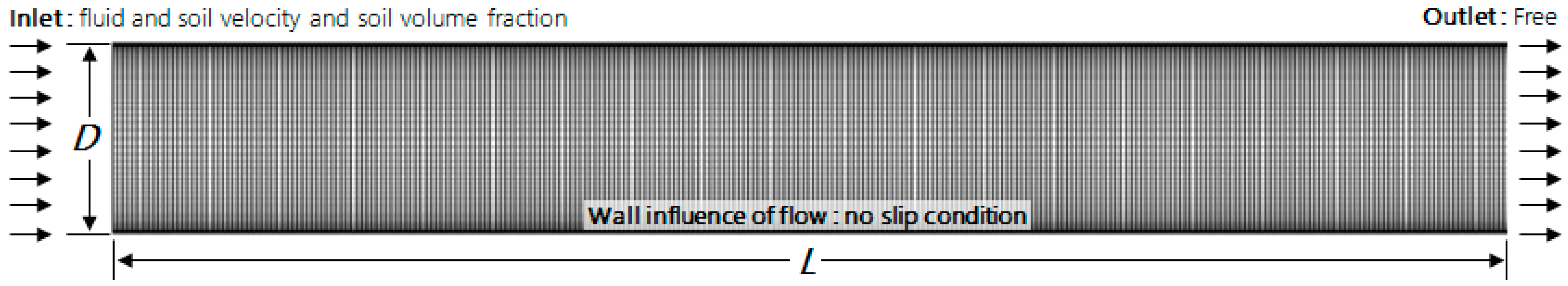
The inlet flow velocity of the soil slurry mixture, the volume concentration of the soil, and its particle size were set as variables. The flow velocity and particle distribution of the mixtures in all 63 conditions were compared and reviewed. Table 3 lists the values of parameters of the fluid and soil slurry mixture, which are similar to those used by Song et al. [23]. To simulate the soil slurry transfer and deposition in urban sewer conduits, short conduits were used, as shown in Figure 1. A mesh structure consisting of 140,000 rectangular meshes, each of 0.6 m in diameter and 10 m in length, was implemented. Wall boundary conditions were applied to confine fluid and soil regions. In viscous flows, the non-slip boundary condition is enforced at walls by default; no symmetrical boundaries were applied but the shape of the entire conduit was represented.
As for the cross-section, the fluid and soil slurry flowed into the initial flow section (0 m), where the flow rate was constant for a certain period (500 s). The sectional volume fraction of the cross-section of the conduit was assumed to be the volume fraction of particles in the total flow. For the outlet (10 m), the results of the flow field and volume fraction in nine sections (1–9 m inside) were reviewed. In the case of the inlet, the flow velocity was constant, and thus flow field could be neglected. In the case of the outlet, the two-phase flow was such that the distribution of the flow field and volume fraction tended to be scattered. Therefore, it was excluded. Shields performed experiments in flumes with widths of 0.8 m and 0.4 m and beds composed of particles with diameters from 0.36 mm to 3.44 mm; mean velocity was increased in steps of 0.1 m/s to 0.6 m/s [13]. Brownlie conducted studies on the Colorado River, Mississippi River, and Red River. In his study, the flow velocity had minimum and maximum values of 0.37 m/s and 2.42 m/s, respectively, and beds were composed of particles ranging from 0.08 mm to 1.44 mm in diameter [15]. In this study, the same specification was applied to a sewer based on a numerical model. In the analysis, the particle size and inflow rate were changed to reflect the runoff condition in actual sewers. The transport and erosion phenomena in the conduit were reviewed. For discharge flowing into sewer pipes, most flow in as a mixture of fluid and soil slurry depending on the occurrence of rainfall, showing characteristics of turbulent flows. Accordingly, for soil slurry flowing into conduits, this study investigated the characteristics of flows inside conduits by determining the rate of flow corresponding to outflow and that to inflow occurred in mixed forms. The soil slurry flowing into the conduit contained particles of different sizes. The slurry was modeled by considering the dispersion of particle size. However, only particle size influenced velocity and particle distribution of the mixture. Therefore, we assumed particles of uniform size by considering a single particle size [23].
2.4. Model Validation
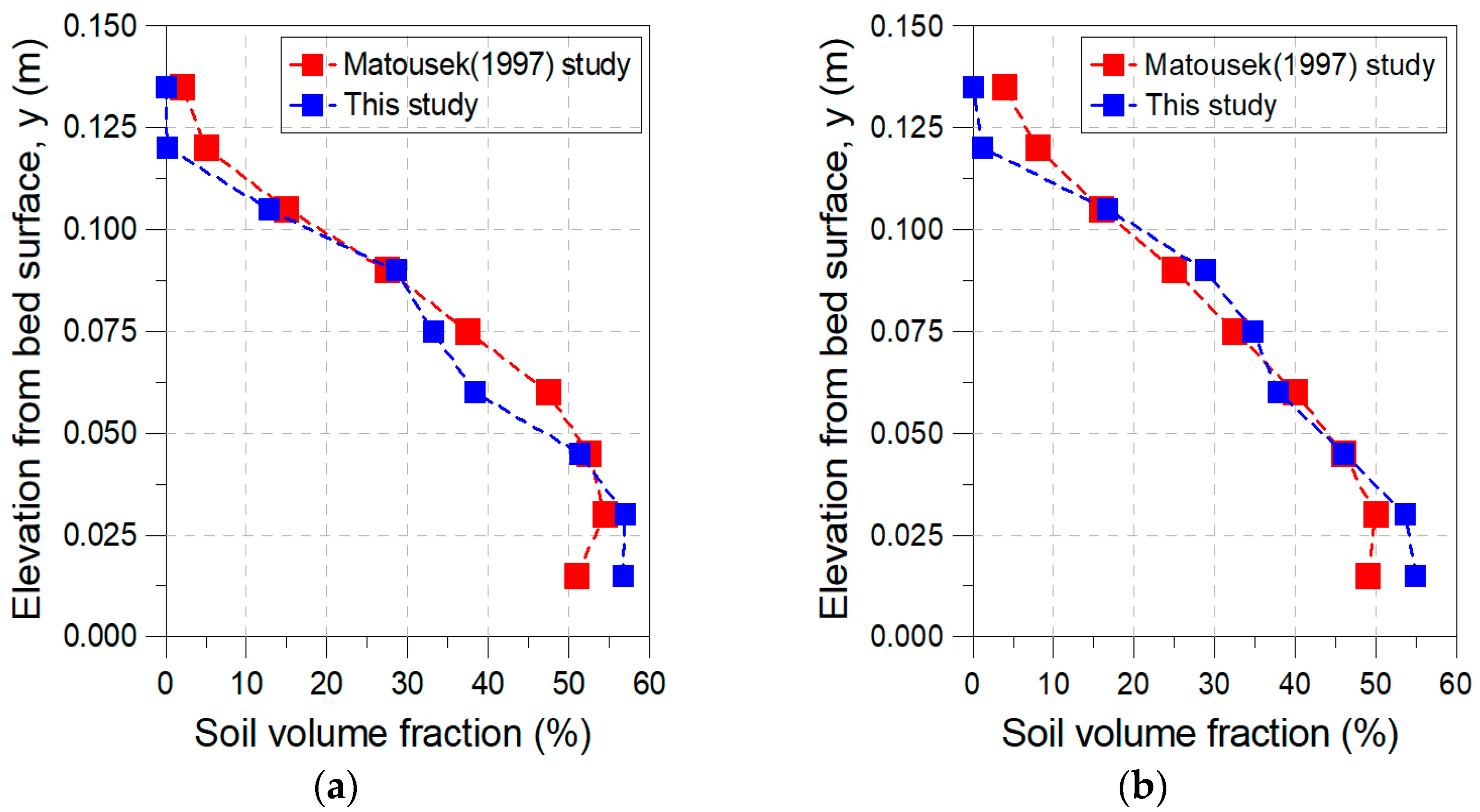
Song et al. [23] developed a model based on the experimental results obtained by Nabil et al. [43]. Based on the correction process, they suggested that the distribution of flow velocity and the changing pattern of the volume fraction of soil slurry were consistent in a conduit in their model. They reported experimental results for soil particles 1.4–2.0 mm in size, as used by Matousek [44].
Figure 2 shows the transfer of particles of size 1.4–2.0 mm in urban sewer conduits, with a volume concentration of 26% and flow velocities of 2.5 m/s and 3.0 m/s. A significant of the resulting flow was consistent. The internal distribution under the two conditions of flow velocity and volume concentration, which were used for examination, tended to be the same. Therefore, the analysis model was considered verified.
3. Numerical Modeling
3.1. Analysis of Flow Characteristics in Conduit Depending on Inlet Flow Velocity
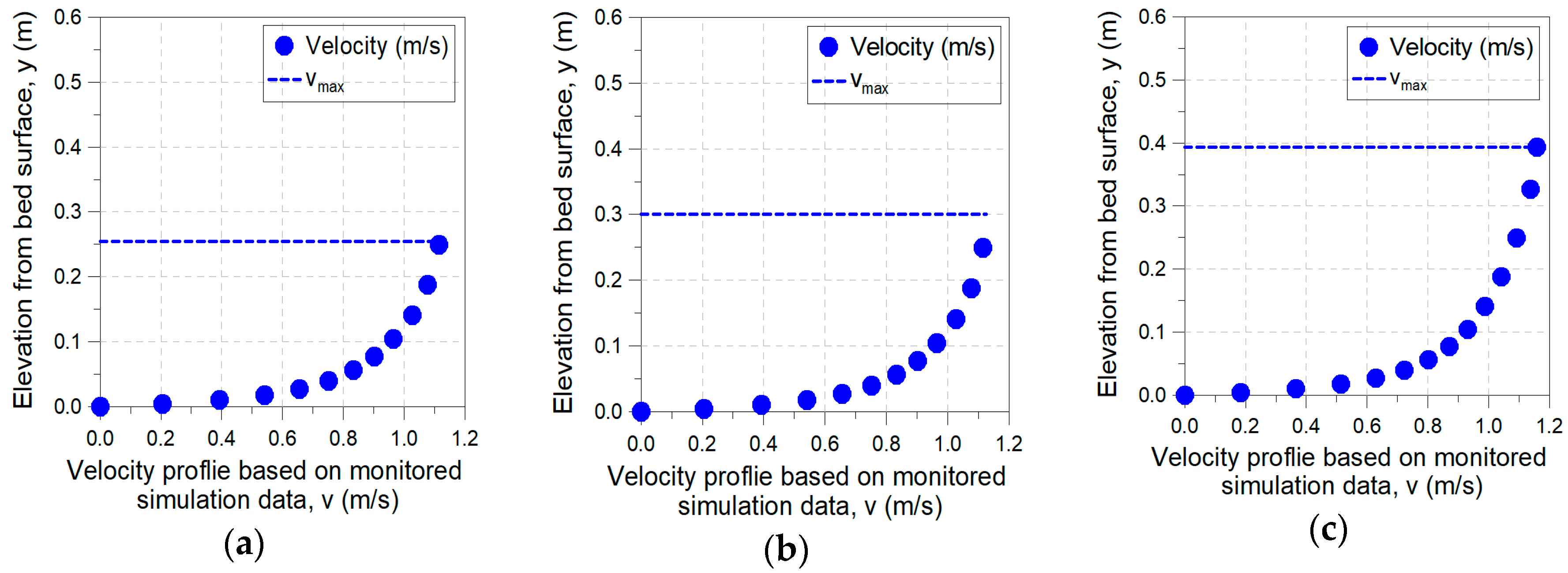
The transfer of soil slurry in a conduit influences flow velocity under the action of inertia and gravity. Figure 3 and Figure 4 show changes in the flow velocity in a conduit depending on the volume fraction at the same flow velocity for 1.0 mm and 20.0 mm of slurry. As shown in Figure 3, in the case of the flow velocity distribution of a single fluid, the flow velocity converged to zero at the bottom of the conduit, and then assumed the maximum value at the center with a rise in the diffusion coefficient through the volume fraction grade of soil slurry. However, this study analyzes two-phase flow rather than that of a single fluid, and revealed that the maximum value of flow velocity increased in the upper part of the conduit with changes in the volume fraction. The maximum flow velocity should have been observed at the center of the conduit because of the soil slurry deposited at its bottom.
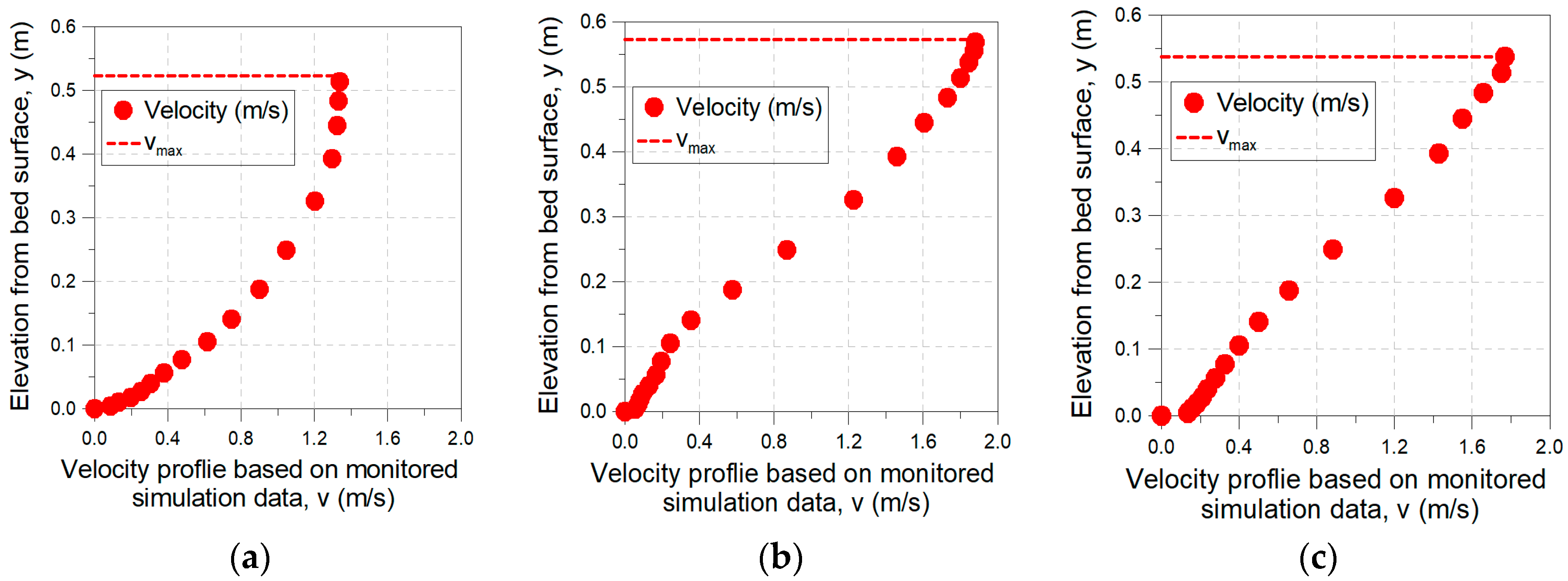
In Figure 4, the flow velocity at the bottom changes slowly because of the soil slurry. In the upper part of the conduit, where the volume fraction had been reduced, the flow velocity tended to increase. With a rise in the volume fraction of the soil slurry in the lower part of the conduit, the damping effect of turbulence due to fluid friction largely worked and, consequently, the maximum value of flow velocity moved to the upper part of the conduit. Depending on deposition, the volume fraction of the soil slurry in the upper part of the conduit was smaller than that in the lower part. It was analyzed to be ideally consistent with the flow of a single fluid.
The distributions of the flow velocity of 1.0 mm and 20.0 mm of slurry were used in this study to verify that relatively smaller particles changed rapidly in the lower part of the conduit with a large volume fraction of soil slurry. It is fair to attribute this result to relative density. In general, the higher the volume fraction of soil slurry, the greater the interaction of particles in the mixture and the higher their viscosity. As a result, the flow velocity of the fluid in a relevant section decreases and, if the volume fraction decreases, flow velocity increases.
3.2. Analysis of Flow Characteristics of Conduit Depending on Inlet Volume Fraction
The most significant change with changing volume fraction of the inlet occurred in the distribution of flow velocity in the conduit. The volume fraction influenced the flow of each particle and changed the distribution of the flow velocity. The homogeneity of the distribution of flow velocity thus represented the homogeneity of the particle distribution. Figure 5 and Figure 6 show the changes depending on volume fraction at velocities of 1.0 mm and 20.0 mm of the slurry. As shown in the results, the volume fraction in the upper part was close to zero, and a large volume fraction was observed only in the lower part of the conduit. The frictional force arising in the lower part did not significantly influence the center of the conduit with the maximum turbulence and flow velocity.
Figure 5 shows the influence of the particle size of the soil slurry. As shown, when particle diameter was small, the distribution of volume fraction altered from heterogeneous to homogeneous along with a change in flow velocity. When the particles were small, they were easily moved by the eddy of the fluid. As shown in Figure 6, this was because particle movement was determined by gravity, which is based on unit particle weight. In general, with an increase in flow velocity, the fluid force became greater than the resistance of the hardened deposit and, thereby, moved the soil slurry. Friction increased with rising tractive force. Based on the change in flow velocity observed at the bottom of the conduit, the limiting tractive force could be estimated by calculating the shear flow velocity and shear stress in the conduit.
To sum up the numerical analysis, the larger the particle size of the soil slurry and the greater the increase in volume fraction, the greater the deposition. The higher the flow velocity, the smaller the deposition. An increase in the layer deposited led to increased flow velocity in the upper part of the conduit. With increased particle size of the soil slurry, deposition was evident.
4. Functional Relationship of Soil Slurry Transfer Deposition in Urban Sewer Conduits
4.1. Calculation and Review of Limiting Tractive Force
The major parameters needed to determine transfer deposition in the fluid transfer process are the vertical distribution of soil slurry in the conduit and the shear flow velocity () along the floor boundary. The shear flow velocity causes the soil slurry deposited at the bottom of the conduit to float in the re-floating process. At this time, the volume concentration can induce a smooth transfer or re-sedimentation. Accordingly, the shear flow velocity influenced by the layer of deposit was reviewed to measure the change in shear flow velocity at the bottom of the conduit. In general, this change in shear flow velocity represents a change in kinetic energy.
The characteristics of soil slurry include physical, such as particle size (d), density () and settling velocity (), and volumetric constituents, such as the volume fraction of flow and the unit weight of mixed fluid flow. Raudkivi claimed that sediment transfer depends on shearing speed and the relative particle settling velocity [45]. Shearing speed can be calculated using Equations (9) and (10), and the settling velocity of the particle can be calculated using Equation (11). Shear stress is calculated through conversion. is the specific gravity of the sediment (submerged) in fluid, is its density (kg/m3), is the density of water (kg/m3), g is the acceleration due to gravity (m/s2), d the particle diameter (m), and is the coefficient of drag, which varies depending on the free motion of a particle but generally converges to 0.44 in turbulent flow. It is known that the drag coefficient of particles in a turbulent fluid may be significantly different, depending on concentrations and particle characteristics. The viscosity of the mixture, however, increases rapidly with volumetric sand concentrations beyond 20% [46,47]. For mixture flow, pressure drops could not be predicted accurately. The amount of error increased rapidly with the slurry concentration. These problems will be addressed through further research. The objective of this study is to provide a better description of the physical properties in agreement with numerical data. Accordingly, the average drag coefficient was considered to be 0.44 of a perfect sphere with the same volume and density depending on the particle diameter. Therefore, it was assigned a fixed value without any separate calculation. The particle settling velocity to be applied in this study was calculated using Equation (11). The weight of a submerged particle was calculated by . Subsequently, calculations using particle size could be performed with .
Given the distribution of flow velocity in a certain cross-section, such as flow in the conduit, Shear flow velocity in Equation (12) could be calculated, where is the average flow velocity at the upper distance z relative to the bottom, zo is the distance from the bottom, where the flow velocity is zero, is the flow shear speed, and is the von Kármán constant, which is approximately 0.41 [48,49]. In the case of shear flow velocity using Equation (12), assuming a certain flow velocity distribution in a certain cross-section, an approximate value of velocity can be estimated using the equation below. It can also be calculated using the law of the wall, which was used to explain the relatively thin layer 0.2) at the bottom [29].
Therefore, by applying the change owing to an increase in continuous velocity occurring along the boundary of the bottom of the conduit, the shear flow velocity and shear stress in transfer deposition can be calculated. If y increases discontinuously at a certain calculation point, in Equation (13) increases infinitely. Therefore, the shear stress at the point where there is no change in flow velocity can be defined as the limiting shear stress. In Equation (13), is the dynamic viscosity of the fluid. Shear force is the value of friction generated along the side wall due to the velocity of fluid flow in a cross-section of the conduit. Therefore, this friction is proportional to flow velocity and inversely proportional to the cross-sectional area of a conduit, and is used as shear rate or shear stress. In Equation (13), represents shear stress at the bottom. In Equation (14), is the critical shear stress at the bottom to initiate motion in the sedimentation layer (z) in the conduit, and is used to calculate the limiting tractive force that forms the basis of transfer deposition.
Table 4 lists the results of shear stress based on shear flow velocity in 63 cases. Soil slurry of 0.5 mm diameter had a shear stress of 0.030–0.060 at a velocity of 1–2 m/s. Although there were slight deviations, it generally remained stable at 0.043. At a velocity of 3 m/s, the soil slurry had a value of over 0.284, which means that at relatively high flow velocity, the soil slurry was deposited more rapidly at the bottom of the conduit. Given that the amount of soil slurry (flow amount defined as the mass of soil slurry per total volume in unit flow) flowed in proportion to the inlet flow velocity, a larger deposit was expected when a large amount of slurry flowed in. This means that small particles could be deposited in the conduit. Soil slurry of 20.0 mm diameter had an average value of 0.053, which was maintained even with changes in flow velocity. The probability of sedimentation based on deposition was 0.056, the value suggested by Shields [13]. Given these results, if particle size increased, the density and specific gravity of the soil slurry increased. Deposition thus easily occurred and the settling velocity increased.
Shear flow velocity and shear stress at the bottom represent the force accompanying and transferring the deposits. The shear stress along the critical boundary or the critical erosion speed is the limiting condition of deposit transfer and shear stress (limiting point of motion) at the start of the yield. The value of roughness at the bottom depends on the size of sediment particles there, and influences changes in the flow velocity distribution and the transfer capability of the soil slurry.
In general, the settling velocity influences the movement of the particles once the dynamic force of the fluid is imposed on them, and thus creates a boundary layer. In turbulent flow, if the flow velocity increases, the amount of force on the particles exceeds a threshold and acts on the sediment particles at the bottom of the conduit under a constant velocity. This means that, when the threshold is reached, shear stress in the conduit dominates the transfer velocity of the deposits, and significantly depends on flow velocity.
4.2. Functional Relationship of Transfer Deposition Due to Soil Slurry Particles
The method proposed by Shields [13] is commonly used to calculate the limiting tractive force as it can be used to directly compare the results obtained at different densities and viscosities, and thus makes it possible to easily judge the conditions of flow. However, in this method, the velocity of shear flow and the size of particles belong to both the longitudinal and transverse axes, and thus, the relationship between them is unclear. Therefore, the limiting tractive force for a given particle size could not be directly calculated. Problems and improvements regarding Shields’ methodology have been discussed by Maa [50], Yalin and Karahan [51], and Smith and Cheung [52]. To solve these problems, Julien introduced a dimensionless parameter given by and proposed the following modified Equation (15) [14]. is defined as exactly analogous to Rouse’s auxiliary parameter or Rouse Reynolds number, eliminating the critical shear stress from the abscissa definition (in Reynolds number coordinates) [53]. Here, “SPG” represents the specific gravity of the particle. The Reynolds number for a multiparticle system, given in Equation (16), is defined in a similar manner as a function of the void fraction [54,55].
The works by Shields, Brownlie, and Parker et al. have improved and applied the limited diameter-based equation. To review the case where the limited diameter is small, this study used the results of a numerical analysis [15,56].
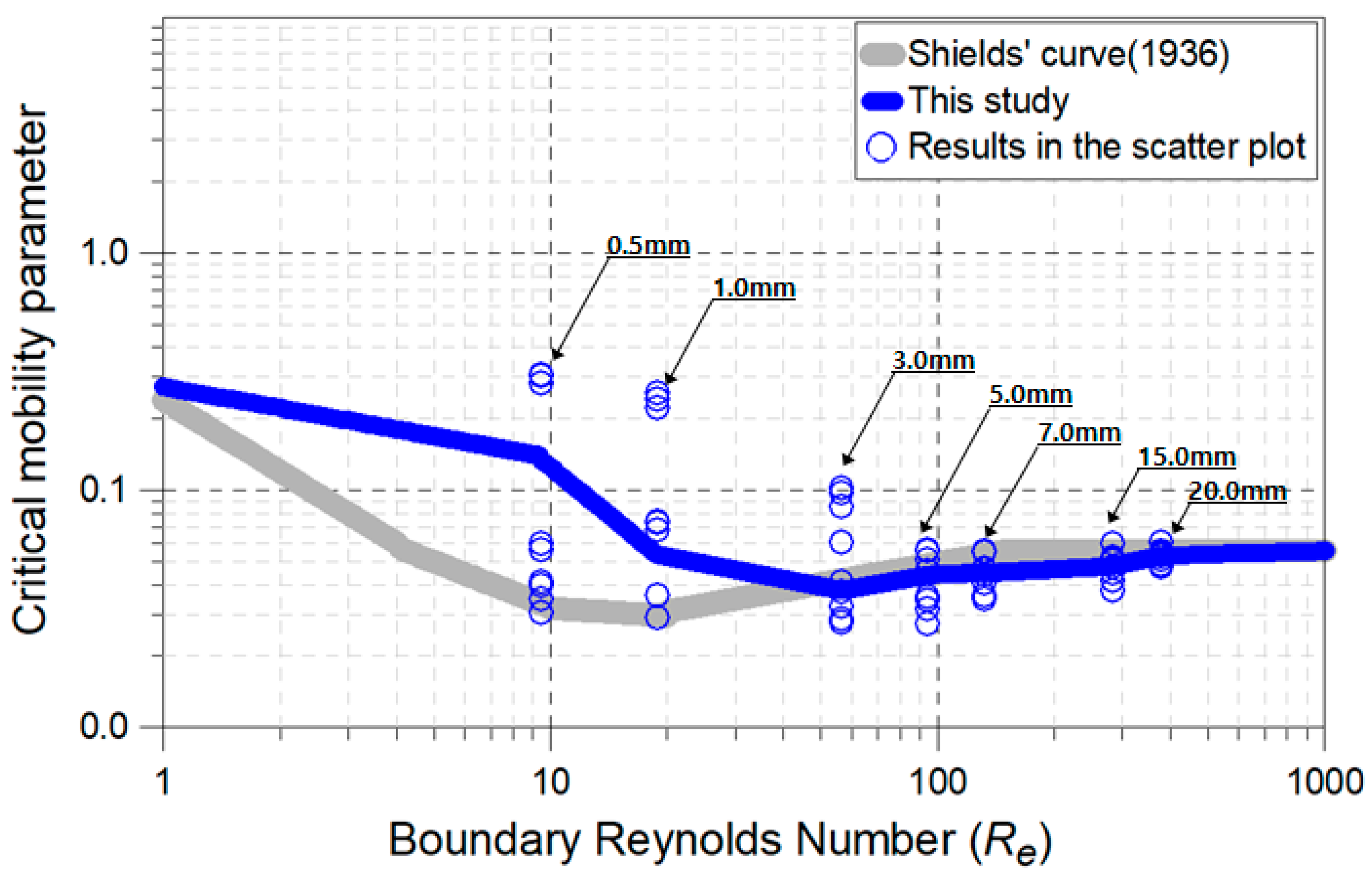
The results for particles of sizes 0.5–20.0 mm are presented without dimensions and compared with the results reported by Shields’ limiting tractive force as shown in Figure 7. Shields used 15 data items, whereas this study used 63 for comparison.
As shown in Figure 7, the limiting tractive force for relatively smaller particles (0.5 mm and 1.0 mm) was close to the criteria suggested by Shields’ curve. A velocity of 1.0 m/s was obtained for consistent conditions. The pattern of the increasing amount of soil slurry flowing with increased flow velocity was different from that in Shields’ diagram. The range of limiting tractive force was 0.224–0.307, which means that with increasing flow velocity, the inflow of a large amount of soil slurry led to higher sedimentation. In a turbulent state, high flow velocity leads to a more active deposition of particles, which means that small particles can be deposited in the conduit.
With increasing particle size, a pattern similar to that in Shields’ diagram was observed. In the case of a relatively larger particle of diameter of 20.0 mm, the variable for transfer deposition was calculated to be 0.053, identical to the result suggested by Shields’ curve even with changes in flow velocity. This means that, if the particle size increased, the density and specific gravity of the soil slurry also increase, and particles are rapidly deposited at the bottom of the conduit regardless of the values of other variables. Therefore, particle size is the basic criterion for soil slurry transfer in calculating the limiting tractive force, but its influence is considered to be little to negligible if particle size is greater or less than a particular value. Small particles flowing into an urban sewer conduit constitute an important variable, and, thus, the conduit must be designed considering its discharge capacity.
To account for measurement errors in Table 5, the evaluation accuracy was examined by calculating two different evaluation statistics: SSQ (the sum of the squares) and RMSE (root mean squared error). These are expressed as Equations (17) and (18).
where is the amount of observed values, is the amount of calculated values (Table 5), subscript i indicates its data in the set, and is the number of data [57,58,59,60]. The results of the numerical model were compared with those of Shields and Brownlie [13,15]. To measure errors, we compared the values obtained in Table 5 with those of Shields and Brownlie, as shown in Table 6.
The overall SSQ and RMSE values were found to be 0.0020 and 0.0446, respectively. Theoretically, a functional relationship equation is accepted as excellent when RMSE and SSQ values are equal to zero. The RMSE and SSQ values in this study indicate that the assessed results were highly correlated. Accordingly, this study proposed a functional relationship of the limiting tractive force for particles of different sizes, as shown in Table 5. The functional relationship can be used as the criterion to assess the transfer deposition of soil slurry in a conduit. The modified equation proposed in this study expresses this criterion and can be used to calculate the amount of sedimentation in a conduit.
Nevertheless, further studies should focus on analyzing errors considering various diameters and mathematical representation of the curve of critical tractive force results, such as flow conditions and other derived particle parameters.
5. Conclusions
In this study, a numerical analysis was performed to investigate the influence of the transfer deposition of soil slurry in urban sewer conduits. The results were analyzed based on various flow conditions. Particle size was set as the main parameter and settling velocity was applied to analyze deposition behavior in the conduit. By considering the turbulence model, the shear flow velocity was investigated according to flow velocity and volumetric concentration. Accordingly, a functional relationship used to identify the boundary of the transfer deposition of soil slurry in urban sewer conduits. Based on the entire process of the numerical analysis, the following conclusions can be drawn:
- Particle size is the basic criterion for soil slurry transfer in calculating the limiting tractive force, but its influence is little to negligible if particle size is greater or less than a particular value. Nevertheless, small particles flowing into urban sewer conduits are an important variable, and thus conduits must be designed considering their discharge capacity.
- A turbulence model was applied to calculate average flow velocity, shear flow velocity, and shear stress. In a conduit with sedimentation, the distribution of flow velocity was weakened overall by a similar drag-based volume fraction, and a slant in the flow velocity in the conduit increased due to deposition. The shear flow velocity and turbulent stress were large when a large value was calculated around the boundary of the bottom of the conduit. Therefore, it was estimated by applying an overall inclination.
- Based on the results, the authors proposed a functional relationship between the limiting tractive and particle size. This relationship can be used as criterion to judge the transfer deposition of soil slurry in a conduit, and can be applied to urban sewer conduits, unlike previous studies. If the phenomena in urban sewer conduits are measured for comparison in an improved study, a more reasonable research method can be devised.
- The results of this study can help overcome inaccuracy in simulating particles of small diameters in one-dimensional models, which are used to estimate the flow of sediment in urban sewer conduits. In future work, it will be necessary to further investigate the deposition rate of soil in conduits and the pattern of cohesion of each particle.
The findings of this study may be helpful in designing conduits with the aim of preventing conduit clogging or conduit damage that may occur during heavy rainfall events. To analyze drainage flow under the influence of various soil shapes and floating particles, it is necessary to consider different conditions through model experiments and numerical modeling. This study considered only the inflow of a large amount of soil slurry at the beginning of rainfall events. Therefore, the proposed method must be further investigated by introducing various types of rainfall events. Moreover, to validate the results of this study, data from real conduit systems must be collected and analyzed using a rainfall–runoff model. Overall, further research is required to determine the relationship considering the volume fraction of small particles.
Author Contributions
Y.H.S. carried out the literature survey and wrote the draft of the manuscript. Y.H.S. and E.H.L. worked on subsequent drafts of the manuscript. Y.H.S. and J.H.L. performed the simulations. Y.H.S., E.H. and J.H.L. conceived the original idea of the proposed method.
Funding
This research was supported by a grant (MOIS-DP-2015-03) from the Disaster and Safety Management Institute funded by the Ministry of Interior and Safety of Korea.
Acknowledgments
This research was supported by a grant (MOIS-DP-2015-03) from the Disaster and Safety Management Institute funded by the Ministry of Interior and Safety of Korea
Conflicts of Interest
The authors have no conflict of interest to declare.
References
- Chebbo, G.; Gromaire, M.C.; Ahyerre, M.; Garnaud, S. Production and transport of urban wet weather pollution in combined sewer systems: The “Marais” experimental urban catchment in Paris. Urban Water 2001, 3, 3–15. [Google Scholar] [CrossRef]
- Gromaire, M.C.; Garnaud, S.; Saad, M.; Chebbo, G. Contribution of different sources to the pollution of wet weather flows in combined sewers. Water Res. 2001, 35, 521–533. [Google Scholar] [CrossRef]
- Ab. Ghani, A.; Md. Azamathulla, H. Gene-expression programming for sediment transport in sewer pipe systems. J. Pipeline Syst. Eng. Pract. 2010, 2, 102–106. [Google Scholar] [CrossRef]
- Azamathulla, H.M.; Ghani, A.A.; Fei, S.Y. ANFIS-based approach for predicting sediment transport in clean sewer. Appl. Soft Comput. 2012, 12, 1227–1230. [Google Scholar] [CrossRef] [PubMed] [Green Version]
- Shu, A.P.; Wang, L.; Zhang, X.; Ou, G.Q.; Wang, S. Study on the formation and initial transport for non-homogeneous debris flow. Water 2017, 9, 253. [Google Scholar] [CrossRef]
- Lee, H.Y.; Lin, Y.T.; Yunyou, J.; Wenwang, H. On three-dimensional continuous saltating process of sediment particles near the channel bed. J. Hydraul. Res. 2006, 44, 374–389. [Google Scholar] [CrossRef]
- Li, X.; Wei, X. Analysis of the relationship between soil erosion risk and surplus floodwater during flood season. J. Hydrol. Eng. 2013, 19, 1294–1311. [Google Scholar] [CrossRef]
- Meyer-Peter, E.; Müller, R. Formulas for bed-load transport; appendix 2. In Proceedings of the 2nd Meeting of the International Association for Hydraulic Structures Research (IAHSR), Delft, The Netherlands, 7 June 1948; IAHR: Stockholm, Sweden, 1948. [Google Scholar]
- Song, Z.; Liu, Q.; Hu, Z.; Li, H.; Xiong, J. Assessment of sediment impact on the risk of river diversion during dam construction: A simulation-based project study on the Jing River, China. Water 2018, 10, 217. [Google Scholar] [CrossRef]
- Ribberink, J.S. Bed-load transport for steady flows and unsteady oscillatory flows. Coast. Eng. 1998, 34, 59–82. [Google Scholar] [CrossRef]
- Ungar, J.E.; Haff, P.K. Steady-state saltation in air. Sedimentology 1987, 34, 289–299. [Google Scholar] [CrossRef]
- Joshi, S.; Xu, Y.J. Bedload and suspended load transport in the 140-km reach downstream of the Mississippi River avulsion to the Atchafalaya River. Water 2017, 9, 716. [Google Scholar] [CrossRef]
- Shields, A. Application of Similarity Principles, and Turbulence Research to Bed-Load Movement; California Institute of Technology: Pasadena, CA, USA, 1936. [Google Scholar]
- Julien, P.Y. Erosion and Sedimentation; Cambridge University Press: New York, NY, USA, 1995. [Google Scholar]
- Brownlie, W.R. Prediction of Flow Depth and Sediment Discharge in Open Channels; W. M. Keck Laboratory of Hydraulics and Water Resources, California Institute of Technology: Pasadena, CA, USA, 1981. [Google Scholar]
- Eaton, J.K.; Johnston, J.P. A review of research on subsonic turbulent flow reattachment. AIAA J. 1981, 19, 1093–1100. [Google Scholar] [CrossRef]
- Agelinchaab, M.; Tachie, M.F. PIV study of separated and reattached open channel flow over surface mounted blocks. J. Fluids Eng. 2008, 130, 1–9. [Google Scholar] [CrossRef]
- Brevis, W.; García-Villalba, M.; Niño, Y. Experimental and large eddy simulation study of the flow developed by a sequence of lateral obstacles. Environ. Fluid Mech. 2014, 14, 873–893. [Google Scholar] [CrossRef]
- Georgoulas, A.N.; Kopasakis, K.I.; Angelidis, P.B.; Kotsovinos, N.E. Numerical investigation of continuous, high-density turbidity currents response, in the variation of fundamental flow controlling parameters. Comput. Fluids 2012, 60, 21–35. [Google Scholar] [CrossRef] [Green Version]
- Chuanjian, M.A.N.; Jungsun, O.H. Stochastic particle based models for suspended particle movement in surface flows. Int. J. Sediment Res. 2014, 29, 195–207. [Google Scholar]
- Pang, A.L.J.; Skote, M.; Lim, S.Y.; Gullman-Strand, J.; Morgan, N. A numerical approach for determining equilibrium scour depth around a mono-pile due to steady currents. Appl. Ocean Res. 2016, 57, 114–124. [Google Scholar] [CrossRef]
- Coker, E.H.; Van Peursem, D. The Erosion of horizontal sand slurry pipelines resulting from inter-particle collision. Wear 2017, 400–401, 74–81. [Google Scholar] [CrossRef]
- Song, Y.H.; Yun, R.; Lee, E.H.; Lee, J.H. Predicting sedimentation in urban sewer conduits. Water 2018, 10, 462. [Google Scholar] [CrossRef]
- ANSYS. ANSYS Fluent 12.1 Theory Guide; ANSYS Inc.: Canonsburg, PA, USA, 2010. [Google Scholar]
- Newton, C.H.; Behnia, M. Numerical calculation of turbulent stratified gas–liquid pipe flows. Int. J. Multiph. Flow 2000, 26, 327–337. [Google Scholar] [CrossRef]
- Ghorai, S.; Nigam, K.D.P. CFD modeling of flow profiles and interfacial phenomena in two-phase flow in pipes. Chem. Eng. Process. Process Intensif. 2006, 45, 55–65. [Google Scholar] [CrossRef]
- De Schepper, S.C.; Heynderickx, G.J.; Marin, G.B. CFD modeling of all gas-liquid and vapor-liquid flow regimes predicted by the Baker chart. Chem. Eng. J. 2008, 138, 349–357. [Google Scholar] [CrossRef]
- Bhramara, P.; Rao, V.D.; Sharma, K.V.; Reddy, T.K.K. CFD analysis of two phase flow in a horizontal pipe-prediction of pressure drop. Momentum 2009, 10, 476–482. [Google Scholar]
- Nezu, I.; Nakagawa, H.; Jirka, G.H. Turbulence in open-channel flows. J. Hydraul. Eng. 1994, 120, 1235–1237. [Google Scholar] [CrossRef]
- Durán, O.; Andreotti, B.; Claudin, P. Turbulent and viscous sediment transport—A numerical study. Adv. Geosci. 2014, 37, 73–80. [Google Scholar] [CrossRef]
- Guo, J.; Mohebbi, A.; Zhai, Y.; Clark, S.P. Turbulent velocity distribution with dip phenomenon in conic open channels. J. Hydraul. Res. 2015, 53, 73–82. [Google Scholar] [CrossRef]
- Park, C.W.; Hong, C.H. User Guide of ANSYS Workbench; Intervision: Seoul, Korea, 2008. [Google Scholar]
- Anjum, N.; Ghani, U.; Ahmed Pasha, G.; Latif, A.; Sultan, T.; Ali, S. To investigate the flow structure of discontinuous vegetation patches of two vertically different layers in an open channel. Water 2018, 10, 75. [Google Scholar] [CrossRef]
- Török, G.T.; Baranya, S.; Rüther, N. 3D CFD modeling of local scouring, bed armoring and sediment deposition. Water 2017, 9, 56. [Google Scholar] [CrossRef]
- Fan, F.; Liang, B.; Li, Y.; Bai, Y.; Zhu, Y.; Zhu, Z. Numerical investigation of the influence of water jumping on the local scour beneath a pipeline under steady flow. Water 2017, 9, 642. [Google Scholar] [CrossRef]
- Loth, E.; Kailasanath, K.; Löhner, R. Supersonic flow over an axisymmetric backward-facing step. J. Spacecr. Rocket. 1992, 29, 352–359. [Google Scholar] [CrossRef]
- Sahu, J.; Heavey, K.R. Numerical investigation of supersonic base flow with base bleed. J. Spacecr. Rocket. 1997, 34, 62–69. [Google Scholar] [CrossRef]
- Jalali, P. Theory and Modelling of Multiphase Flows; Lecture Material; Lappeenranta University of Technology: Lappeenranta, Finland, 2010. [Google Scholar]
- Wallis, G.B. One-Dimensional Two-Phase Flow; McGraw-Hill Book Company: New York, NY, USA, 1969. [Google Scholar]
- Launder, B.E.; Spalding, D.B. The numerical computation of turbulent flows. In Numerical Prediction of Flow, Heat Transfer, Turbulence and Combustion; Pergamon Press: New York, NY, USA, 1983; pp. 96–116. [Google Scholar]
- Versteeg, H.K.; Malalasekera, W. An Introduction to Computational Fluid Dynamics: The Finite Volume Method; Pearson Education: London, UK, 2007. [Google Scholar]
- Prandtl, L. Bericht uber Untersuchungen zur ausgebildeten Turbulenz. Z. Angew. Math. Mech. 1925, 5, 136–139. [Google Scholar]
- Nabil, T.; El-Sawaf, I.; El-Nahhas, K. Sand-water slurry flow modelling in a horizontal pipeline by computational fluid dynamics technique. Int. Water Technol. J. 2014, 4, 13. [Google Scholar]
- Matousek, V. Flow Mechanism of Soil–Water Mixtures in Pipelines. Ph.D. Thesis, Delft University, Delft, The Netherlands, 15 December 1997. [Google Scholar]
- Raudkivi, A.J. Loose Boundary Hydraulics, 4th ed.; CRC Press: Rotterdam, The Netherlands, 1998. [Google Scholar]
- O’Brien, J.S.; Julien, P.Y. Laboratory analysis of mudflow properties. J. Hydraul. Eng. 1988, 114, 877–887. [Google Scholar] [CrossRef]
- Wichtmann, T.; Niemunis, A.; Triantafyllidis, T. Strain accumulation in sand due to drained uniaxial cyclic loading. In Cyclic Behaviour of Soils and Liquefaction Phenomena; Taylor & Francis Group: London, UK, 2004; pp. 233–246. [Google Scholar]
- Nezu, I. Experimental Study on Secondary Currents in Open Channel Flows. In Proceedings of the 21st IAHR Congress, Melbourne, Australia, 13–18 August 1985. [Google Scholar]
- Schlichting, H.; Gersten, K.; Krause, E.; Oertel, H.; Mayes, K. Boundary-Layer Theory; McGraw-Hill Book Company: New York, NY, USA, 1955. [Google Scholar]
- Maa, J.P.Y. The bed shear stress of an annular sea-bed flume. In Estuarine Water Quality Management; Springer: Berlin/Heidelberg, Germany, 1990. [Google Scholar]
- Yalin, M.S.; Karahan, E. Inception of sediment transport. J. Hydraul. Div. 1979, 105, 1433–1443. [Google Scholar]
- Smith, D.A.; Cheung, K.F. Initiation of motion of calcareous sand. J. Hydraul. Eng. 2004, 130, 467–472. [Google Scholar] [CrossRef]
- Guo, J. Hunter rouse and shields diagram. In Advances in Hydraulics and Water Engineering; World Scientific Publishing Co.: Singapore, 2002; Volumes I & II, pp. 1096–1098. [Google Scholar]
- Syamlal, M.; O’Brien, T.J. The Derivation of a Drag Coefficient Formula from Velocity-Voidage Correlations; Technical Note; US Department of Energy, Office of Fossil Energy, NETL: Morgantown, WV, USA, 1987. [Google Scholar]
- Wen, C.Y.; Yu, Y.H. A generalized method for predicting the minimum fluidization velocity. AIChE J. 1966, 12, 610–612. [Google Scholar] [CrossRef]
- Parker, G.; Toro-Escobar, C.M.; Ramey, M.; Beck, S. Effect of floodwater extraction on mountain stream morphology. J. Hydraul. Eng. 2003, 129, 885–895. [Google Scholar] [CrossRef]
- Karahan, H.; Gurarslan, G.; Geem, Z.W. Parameter estimation of the nonlinear Muskingum flood-routing model using a hybrid harmony search algorithm. J. Hydrol. Eng. 2012, 18, 352–360. [Google Scholar] [CrossRef]
- Hyndman, R.J.; Koehler, A.B. Another look at measures of forecast accuracy. Int. J. Forecast. 2006, 22, 679–688. [Google Scholar] [CrossRef] [Green Version]
- Willmott, C.J.; Matsuura, K. On the use of dimensioned measures of error to evaluate the performance of spatial interpolators. Int. J. Geogr. Inf. Sci. 2006, 20, 89–102. [Google Scholar] [CrossRef]
- Pontius, R.G.; Thontteh, O.; Chen, H. Components of information for multiple resolution comparison between maps that share a real variable. Environ. Ecol. Stat. 2008, 15, 111–142. [Google Scholar] [CrossRef]
Figure 1.
2D mesh containing 140,000 cells.

Figure 2.
Results of examination using data obtained by Matousek. Results corresponding to flow velocities of: (a) 2.5 m/s; and (b) 3.0 m/s.
Figure 2.
Results of examination using data obtained by Matousek. Results corresponding to flow velocities of: (a) 2.5 m/s; and (b) 3.0 m/s.

Figure 3.
Vertical profile of longitudinal flow velocity of 1.0 mm of slurry in a conduit: (a) 1.0 m/s, 10% volume fraction; (b) 1.0 m/s, 30% volume fraction; and (c) 1.0 m/s, 50% volume fraction.
Figure 3.
Vertical profile of longitudinal flow velocity of 1.0 mm of slurry in a conduit: (a) 1.0 m/s, 10% volume fraction; (b) 1.0 m/s, 30% volume fraction; and (c) 1.0 m/s, 50% volume fraction.

Figure 4.
Vertical profile of longitudinal flow velocity of 20.0 mm of slurry in a conduit: (a) 1.0 m/s, 10% volume fraction; (b) 1.0 m/s, 30% volume fraction; and (c) 1.0 m/s, 50% volume fraction.
Figure 4.
Vertical profile of longitudinal flow velocity of 20.0 mm of slurry in a conduit: (a) 1.0 m/s, 10% volume fraction; (b) 1.0 m/s, 30% volume fraction; and (c) 1.0 m/s, 50% volume fraction.

Figure 5.
Vertical profile of the longitudinal volume fraction of 1.0 mm of slurry in the conduit: (a) 1.0 m/s, 10% volume fraction; (b) 1.0 m/s, 30% volume fraction; and (c) 1.0 m/s, 50% volume fraction.
Figure 5.
Vertical profile of the longitudinal volume fraction of 1.0 mm of slurry in the conduit: (a) 1.0 m/s, 10% volume fraction; (b) 1.0 m/s, 30% volume fraction; and (c) 1.0 m/s, 50% volume fraction.

Figure 6.
Vertical profile of the longitudinal volume fraction of 20.0 mm of slurry in the conduit: (a) 1.0 m/s, 10% volume fraction; (b) 1.0 m/s, 30% volume fraction; and (c) 1.0 m/s, 50% volume fraction.
Figure 6.
Vertical profile of the longitudinal volume fraction of 20.0 mm of slurry in the conduit: (a) 1.0 m/s, 10% volume fraction; (b) 1.0 m/s, 30% volume fraction; and (c) 1.0 m/s, 50% volume fraction.

Figure 7.
Shields’ diagram depending on the boundary Reynolds number and comparison results of the particles.
Figure 7.
Shields’ diagram depending on the boundary Reynolds number and comparison results of the particles.


Table 1.
Parameters of the standard k-ε model.
| Parameter | |||||
|---|---|---|---|---|---|
| Value | 0.09 | 1.44 | 1.92 | 1.0 | 1.3 |
Table 2.
Boundary conditions for analysis.
| Classification | Boundary Conditions |
|---|---|
| Multiphase flow | Fluid (water)-Solid (soil) |
| Applied models and flow conditions | Euler–Euler model Standard k-ε model Turbulent flow Unsteady and turbulent |
| Inlet conditions | Inlet velocity Inlet volume fraction Soil diameter |
| Outlet condition | Free fall |
| Wall condition | Non-slip |
| Convergence | 0.001 |
Table 3.
Basic information concerning the parameters for analysis.
| Parameter | Units | Value |
|---|---|---|
| Conduit specification | m | 0.6 (D) × 10 (L) |
| Mesh specification | grid | 140,000 |
| Inlet velocity condition | m/s | 1.0, 2.0, 3.0 |
| Inlet volume fraction condition | % | 10, 30, 50 |
| Fluid density | kg/m3 | 998.2 |
| Fluid kinematic viscosity | Pa·s | 0.001003 |
| Soil density | kg/m3 | 2,650 |
| Soil diameter | mm | 0.5, 1.0, 3.0, 5.0, 7.0, 15.0, 20.0 |
Table 4.
Calculation of shear stress based on results of numerical analysis.
| d (mm) | |||||||||
|---|---|---|---|---|---|---|---|---|---|
| 1.0 m/s | 2.0 m/s | 3.0 m/s | |||||||
| 10% v/f | 30% v/f | 50% v/f | 10% v/f | 30% v/f | 50% v/f | 10% v/f | 30% v/f | 50% v/f | |
| 0.5 | 0.030 | 0.060 | 0.056 | 0.035 | 0.040 | 0.041 | 0.284 | 0.308 | 0.307 |
| 1.0 | 0.036 | 0.036 | 0.029 | 0.074 | 0.730 | 0.068 | 0.224 | 0.259 | 0.243 |
| 3.0 | 0.061 | 0.037 | 0.041 | 0.033 | 0.029 | 0.028 | 0.086 | 0.098 | 0.102 |
| 5.0 | 0.046 | 0.051 | 0.056 | 0.056 | 0.032 | 0.056 | 0.027 | 0.036 | 0.034 |
| 7.0 | 0.047 | 0.047 | 0.036 | 0.045 | 0.047 | 0.041 | 0.035 | 0.055 | 0.056 |
| 15.0 | 0.052 | 0.052 | 0.060 | 0.038 | 0.045 | 0.048 | 0.042 | 0.042 | 0.051 |
| 20.0 | 0.048 | 0.060 | 0.054 | 0.053 | 0.048 | 0.051 | 0.049 | 0.055 | 0.056 |
Table 5.
Functional relationship of transfer deposition in a conduit using particle size.
| (mm) | (non-dimensional) | Relationship Equation |
|---|---|---|
| ≤ 0.5 | ≤ 9.4 | |
| 0.5 < ≤ 1.0 | 9.4 < ≤ 18.8 | |
| 1.0 < ≤ 3.0 | 18.8 < ≤ 56.4 | |
| 3.0 < ≤ 5.0 | 56.4 < ≤ 94.0 | |
| 5.0 < ≤ 7.0 | 94.0 < ≤ 131.6 | |
| 7.0 < ≤ 15.0 | 131.6 < ≤ 282.1 | |
| 15.0 < ≤ 20.0 | 282.1 < ≤ 376.1 | |
| 20.0 < | 376.1 < |
Table 6.
Comparison between the results of this study and those of Shields and Brownlie.
| (mm) | (non-dimensional) | Shields and Brownlie | This Study |
|---|---|---|---|
| 0.5 | 9.4 | 0.0334 | 0.1468 |
| 1.0 | 18.8 | 0.0298 | 0.0600 |
| 3.0 | 56.4 | 0.0419 | 0.0395 |
| 5.0 | 94.0 | 0.0485 | 0.0438 |
| 7.0 | 131.6 | 0.0535 | 0.0450 |
| 15.0 | 282.1 | 0.0556 | 0.0478 |
| 20.0 | 376.1 | 0.0556 | 0.0530 |
| SSQ | 0.0020 | ||
| RMSE | 0.0446 | ||
© 2018 by the authors. Licensee MDPI, Basel, Switzerland. This article is an open access article distributed under the terms and conditions of the Creative Commons Attribution (CC BY) license (http://creativecommons.org/licenses/by/4.0/).
Share and Cite
MDPI and ACS Style
Song, Y.H.; Lee, E.H.; Lee, J.H. Functional Relationship between Soil Slurry Transfer and Deposition in Urban Sewer Conduits. Water 2018, 10, 825. https://doi.org/10.3390/w10070825
AMA Style
Song YH, Lee EH, Lee JH. Functional Relationship between Soil Slurry Transfer and Deposition in Urban Sewer Conduits. Water. 2018; 10(7):825. https://doi.org/10.3390/w10070825
Chicago/Turabian StyleSong, Yang Ho, Eui Hoon Lee, and Jung Ho Lee. 2018. "Functional Relationship between Soil Slurry Transfer and Deposition in Urban Sewer Conduits" Water 10, no. 7: 825. https://doi.org/10.3390/w10070825
Note that from the first issue of 2016, this journal uses article numbers instead of page numbers. See further details here.