Probabilistic Analysis of Extreme Discharges and Precipitations with a Nonparametric Copula Model

Abstract

Urumqi River is an important river in the Xinjiang autonomous region, China, where floods or droughts are the major concerns of the local communities. This river’s discharge is mainly influenced by the natural factors such as precipitation and climates, rather than human activities. This paper quantifies the interdependent structure between Urumqi River’s discharge and precipitation using a nonparametric Copula method. It then analyzes the relationship between the extreme discharges of this river and extreme precipitation of the region. Comparison between simulation result and real data is conducted to verify the rationality of the model. Furthermore, the conditional probabilities of maximum and minimum discharge at different precipitation levels are also investigated using the Copula distribution functions. The results show a strong relationship between large discharge and heavy precipitation in this region. The upper dependence coefficient is nearly 0.6 and the probability of large discharge reaches 0.64 when the rainfall is greater than 159.56 mm. The relationship between small discharge and rainfall is insignificant. The lower dependence coefficient is zero, suggesting that the base flow and snowmelt from Tianshan likely contribute to Urumqi River’s discharge during the dry season.

1. Introduction

Water resources are one of the most important natural resources for the sustainable development of society [1], especially in the arid and semi-arid areas [2,3]. As one of the world’s extreme arid inland areas with the highest water scarcity index, water resources of the Xinjiang autonomous region have been a great concern to China, and many studies have focused on this issue [4,5,6,7,8,9,10]. The Urumqi River, located on the northern slope of Tianshan Mountain, is one of the most important inland rivers in the region. It is the major water resource for Urumqi City, which has a population of more than 3.5 million [6]. The fluctuation of the river flow significantly impacts the social and economic development of the city. The hydrology process in this area, as well as its response to the climate change, has drawn great attention in recent decades, especially the dependence between climate variability and discharge at the upstream of the Urumqi River. While it is a well-known fact that the rainfall and discharge are closely related, it is difficult to quantify their dependency under extreme events, that is, the dependency between heavy rainfall and large discharge, or between the low rainfall and small discharge. The extreme events are of great concerns to water resources managers. Recently developed Copula theory and method have shed light on addressing such issues, thus, we decided to choose the Copula method to investigate the rainfall and discharge under extreme conditions at this region.

The Copula function (a multivariate probability distribution function) proposed by Sklar [11] can thoroughly quantify dependence among the different variables, regardless of the specific marginal distribution of each component, as such, it has often been used to analyze the dependence between extreme values of two variables. The Copulas function was first introduced to hydrology by De Michele and Salvadori [12], and later, several papers were published [13,14,15,16]. Recently, the method has been applied to investigations of the relationship between extreme hydrological and climate events: for examples, droughts analyses [17,18,19,20,21,22]; rainfall analyses [23,24,25,26,27,28,29,30]; flood analyses [30,31,32,33,34,35,36,37]; and analyses of dam overtopping risk [38,39]. These studies used the parametric Copula method but not the nonparametric Copula method. The parametric Copula approaches use commonly adopted Copula functions (such as Gaussian, t, or Archimedean Copula functions) or their linear combinations to estimate the various relationship between hydrological and climate events. This parametric approach is not sufficient for analyzing hydrometeorology because of the complexity and diversity of the process (that is, it is controlled by many factors). For this reason, we introduce a nonparametric approach to estimating the Copula function in the hydrometeorological studies. Since this approach is not constrained by the commonly employed Copula functions, it can yield Copula functions for site-specific datasets, or say, it is a data-adaptive method.

Nonparametric Copulas estimation was originated from Deheuvels (1979) [40], who proposed an estimator on a multivariate empirical distribution based on the marginal empirical distributions. Then Lejeune and Sarda (1992) [41] improved the method to reduce the boundary bias. Later Fermanian and Scaillet (2003) [42] improved the above method, and then Chen and Huang (2007) [43] proposed effective and advanced estimation method, which is approximate unbiased at each interior, boundary and corner points of the support set, and yields small variances. They showed that the estimator is consistent for each point of the support set.

Considering the above advantages, this study used Chen and Huang’s (2007) [43] nonparametric Copula estimation method for the first time to quantify how precipitation impacts the streamflow in mountain drainage basins Specifically, we built the nonparametric Copula function between the discharge and precipitation at this region, developed their joint probability distribution and density functions, and analyzed the dependency structure of the extreme values, including the calculation of upper and lower dependence coefficients. In addition, the performances between non-parametric and parametric Copulas are compared. Simulations were also carried out to verify the rationality of the estimated model. Meanwhile, we explained the mechanism behind the phenomenon based on the estimated Copula joint density and the dependence coefficients and investigated factors controlling the Urumqi River’s discharge at different periods during a year’s period. Subsequently, we used the result to derive the conditional probabilities of the maximum and minimum discharges at various precipitation levels.

2. Field Site and Data

2.1. Field Site

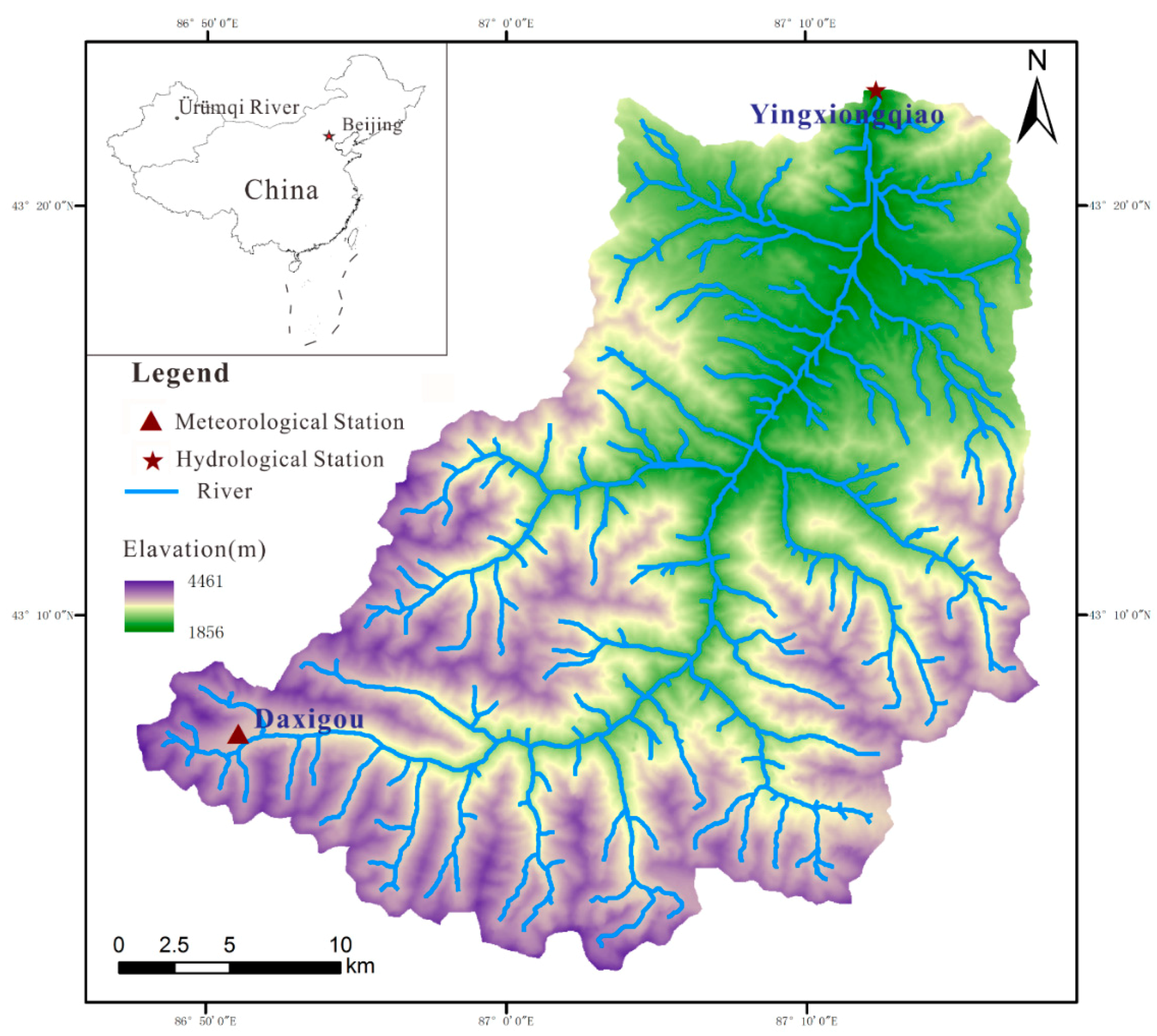
The Urumqi River upstream basin is situated on the south fringe of Junggar Basin, on the north slope of the Tianshan Mountains in Xinjiang, northwest China [7,9]. The basin extends from 43°00′ N to 43°28′ N, and from 86°45′ E to 87°18′ E (Figure 1). The river originated from Glacier No. 1 at an elevation of 3900 m above mean sea level (AMSL), on the northern flank of Tianger Peak II (4479 m AMSL) in the middle Tianshan Mountains [9]. It is a typical inland intermountain river fed by a mixture of the glacier-melt water and precipitation [6,8,44]. The flood along the river occurs in July and August, and it is mainly caused by rainfall. Of course, the snowmelt on the top of the mountain can sometimes aggravate the flood [7,8].

The region has a complex topography, which includes grassland, marsh, and desert in addition to the surrounding mountainous alpine areas [45]. Overall, this basin is poorly gauged. In 1958, the Yingxiongqiao Hydrological Gauging Station (YHGS) (Figure 1) installed gauges to monitor the upstream of Urumqi River. It is the only hydrological gauging station with available data for long the time series located at the mountain pass. As a typical alpine river, the length of the Urumuqi river above the YHGS is about 62.6 km with a drainage area of 924 km² while the altitude range is nearly 2000 m and the averaged gradient is 0.032 [46]. Because of the steepness of the gradient, the velocity of the river is fast, and the discharge that comes from one month’s precipitation will flow away quickly and will not affect the next month’s discharge. Thus, the monthly averaged discharge data can be viewed as independent events or datum (Figure 1).

2.2. Data

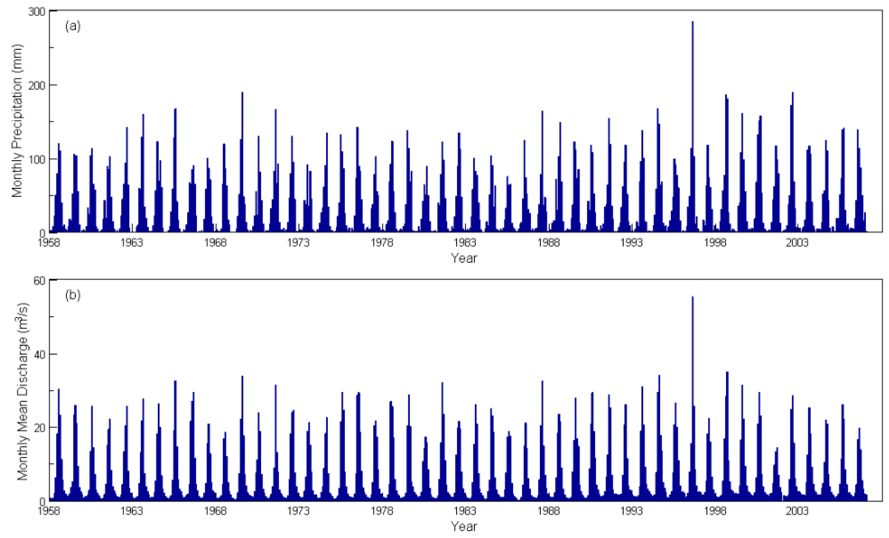
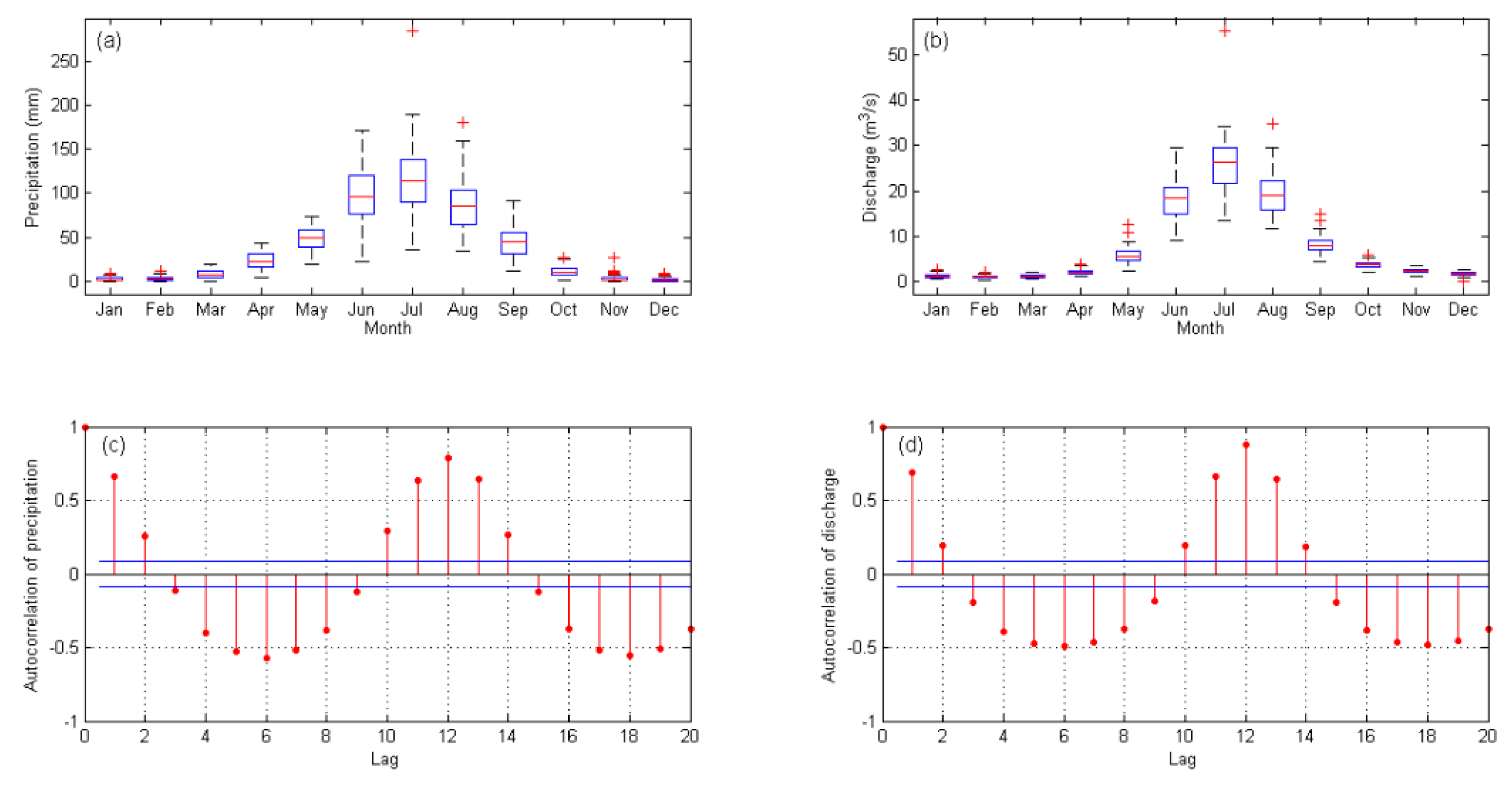
The monthly averaged discharge, and precipitation datasets of Urumqi River from January 1958–December 2006 are used in this study as shown in Figure 2, and the relationship between extreme monthly averaged discharge and precipitation is the main focus of this article. The discharge data is collected from YHGS, and the precipitation data is obtained from Daxigou Meteorological Station (DMS). Both precipitation and discharge exhibit cycle characteristics with the period of one year, and have no long-term trend. The averaged discharge and precipitation are 7.63 m³/s and 37.80 mm, and their standard deviations are 8.74 m³/s and 44.7 mm, respectively. The boxplots of precipitation and discharge for each month and the autocorrelation functions of the two series with lags 1 to 20 are shown in Figure 3. At the upstream of the Urumqi River, precipitation occurs most frequently from June to August, and the annual maximum discharge usually occurs during this period. The observed annual maximum precipitation in the upstream area is 632 mm (in July 1996), and the annual maximum discharge is 55.2 m³/s, which occurs at the same time as precipitation. The rainless season usually occurs from November to the next April, and the minimum discharge usually takes place in December, January, February, or March. From the observation data, the minimum discharge is 0.06 m³/s (at December 2001) while the minimum precipitation is 0 mm, taking place in January 1965, December 1967, and December 1968. The correlation coefficient of precipitation and discharge series is as high as 0.919, which implies the high correlation between the two as we expected. While the correlation coefficient can only measure the linear correlation between the two variables, it cannot provide a detailed joint distribution surface of the two and the relationship between extreme precipitation and discharge, which needs to be further studied by the copula method. It should be noted that the Daxigou Reservoir, located at 5 km upper of YHGS, was constructed in 2007. Its construction disturbed the natural hydrological conditions of upstream of the Urumqi River, and the data of YHGS after 2006 are, thus, excluded in this study.

3. Methods of Analysis

3.1. The Nonparametric Copula Estimator

Let $(X,Y)$ denote a two-dimensional random vector with $F(x,y)$ being its joint distribution function, and $F_1(x)$ and $F_2(y)$ are the marginal distributions of $X$ and $Y$ respectively. Sklar(1959) [11] proved that there exists a unique function $C$ on ${[0,1]}^2$, such that $F(x,y)=C(F_1(x),F_2(y))$ for all $(x,y)$ in the real number field. Both $F_1(X)$ and $F_2(Y)$ have uniform distributions with a support set [0,1], and the function $C$ is a two-dimensional joint distribution function of $F_1(X)$ and $F_2(Y)$, which is called the Copula distribution function of $X$ and $Y$. Then, the Copula joint density function $c(u,v)$ is

$$c(u,v)=\frac{{\partial }^{2}C(u,v)}{\partial u\partial v},(u,v)\in {[0,1]}^2$$

Note that the surfaces of $C(u,v)$ and $c(u,v)$ fully describe the dependence between $X$ and $Y$, after filtering out each one’s marginal distribution. That means the Copula functions remove the respective characteristics of $X$ and $Y$, and highlight their relationship. For hydrometeorology investigation, let $X$ and $Y$ be a hydrological and a meteorological time series respectively. The probability of the concurrence of extreme hydrological and meteorological events, such as heavy precipitation and huge discharge, or little precipitation and small discharge, which are often of our interests, can then be observed by the shape of the Copula density function, $c$, near the corner points (0,0) and (1,1). For instance, if the shape of $c$ is convex upward at the region near (0,0) or (1,1), the possibility that both precipitation and river discharge have a minimum or a maximum value at the same time is high. On the other hand, if the surface of $c$ is flat and close to zero at the region near (0,0) or (1,1), then the probability that both events simultaneously have extreme values is small.

The functions $C$ or $c$ are unknown but can be estimated from the observed data. Chen and Huang (2007) [43] developed a nonparametric procedure to estimate the copula $C$ function, which consists of two stages. The first step is to estimate the marginal distributions functions of $X$ and $Y$, that is, $F_1$ and $F_2$ using commonly used parametric distributions, such as normal, exponential distributions, and so on, or some non-parametric methods such as kernel density estimation or empirical distribution. Because the data used in this paper does not fit the well-known parametric distributions well with almost zeros p values, while the famous kernel density estimation does not have good extrapolation capacity [41], thus, in this paper, we choose the conservative approach, that is, using empirical distribution functions which can deal with interpolation problems only, as approximations of marginal distributions, the expression of which are written as

$${\widehat{F}}_l(s)=\{\begin{array}{l}0\begin{array}{cc},& s<s_{(1)}^l\end{array}\\ \frac{k}{n}\begin{array}{cc},& s_{(k)}^l\le s<s_{(k+1)}^l,k=1,\dots ,n-1\end{array}\\ 1\begin{array}{cc},& s\ge s_{(n)}^l\end{array}\end{array}$$

(1)

where $l=$1 or 2, ${\widehat{F}}_1(s)$ and ${\widehat{F}}_2(s)$ represent the estimations of the marginal distribution functions of $F_1$ and $F_2$ respectively. $n$ is the observation number and $s_{(k)}^1$ denotes the $k$th order statistics of the sample from $X$, and similarly, $s_{(k)}^2$ denotes the $k$th order statistics of the sample from $Y$, then we have $s_{(1)}^l\le s_{(2)}^l\le \cdots \le s_{(n)}^l$.

The second stage is to estimate the function $C$ based on the estimated ${\widehat{F}}_l$s, the details of which are given below.

Let the local linear kernel $K_{u,h}(x)$ defined as

$$K_{u,h}(x)=\frac{K(x)\{a_2(u,h)-a_1(u,h)x\}}{a_0(u,h)a_2(u,h)-a_1^2(u,h)}I(\frac{u-1}{h}<x<\frac{u}{h}),$$

where $K(x)$ is a symmetric probability density function, satisfying that (1) $K(x)$ ≥ 0; (2) ${\displaystyle {\int }_{-\infty }^{+\infty }K(x)=1}$; (3) $K(x)=K(-x)$, for any $x\in R$. $h$ denotes the bandwidth and $h$ > 0. $I(·)$ is an indicator function, which equals to 1 when the logical expression in the brackets is true and otherwise equals to zero. $a_l(u,h)={\displaystyle {\int }_{(u-1)/h}^{u/h}{t}^{l}K(t)dt}$ for $l=$0, 1, 2 [41]; Let $G_{u,h}(t)={\displaystyle {\int }_{-\infty }^t{K}_{u,h}(x)dx}$ and $T_{u,h}=G_{u,h}\{(u-1)/h\}$, then the estimate of Copula distribution function is written as

$$\widehat{C}(u,v)=\frac{1}{n}{\displaystyle \sum _{i=1}^n{G}_{u,h}(\frac{u-{\widehat{F}}_1(X_{i1})}{h})G_{v,h}(\frac{v-{\widehat{F}}_2(X_{i2})}{h})}-(u{T}_{v,h}+v{T}_{u,h}+T_{u,h}{T}_{v,h})$$

(2)

where $\widehat{C}(u,v)$ is the estimator of $C(u,v)$ at the point $(u,v)$. Equation (2) is used in this paper to estimate the Copula function between discharge and precipitation. Chen and Huang (2007) [43] proved that Equation (2) is approximate unbiased and has a small variance.

Subsequently, the Copula density function $c$ can be estimated using Equation (2), that is

$$\widehat{c}(u,v)=\frac{\widehat{C}(u,v)-\widehat{C}(u-\Delta u,v)-\widehat{C}(u,v-\Delta v)+\widehat{C}(u-\Delta u,v-\Delta v)}{\Delta u\Delta v}$$

(3)

where $\Delta u$ and $\Delta v$ are the very small increments of $u$ and $v$ respectively.

3.2. The Explanation of the Reasonability of the Data and Methods Application

Figure 3c,d show that the autocorrelation functions of precipitation and discharge both have long trailing tails, indicating that each of them is related to time, the performance of which is understandable because of the characteristic of monsoon climate in Urumqi, which must be rainy during the summer and less rainy during winter, leading to the periodicities and the correlation with time presented by precipitation and discharge. This is not consistent with the classical statistics which requires that the sample data should be independent and identically distributed. While in fact, all the data pairs of precipitation and discharge used in this paper can also be considered coming from one bivariate population in another point of view, the reasons of which are in the following: It is generally accepted that the precipitation and discharge data from the same month are independent and identical distributed, and we suppose that the joint distribution function of discharge and precipitation in each month is $F_i(x,y)$, $i=1,\dots ,12$, where $x_{}$ is discharge and $y$ is precipitation, and $i$ represent the $i$th month. Then the arithmetic mean of $F_i(x,y)$s, that is, $\frac{1}{12}{\displaystyle {\sum }_{i=1}^{12}{F}_i(x,y)}$ also forms a bivariate joint distribution function, which meets all the theoretical requirements of the joint distribution function. Let us define this distribution function as $F(x,y)$, i.e., $F(x,y)=\frac{1}{12}{\displaystyle {\sum }_{i=1}^{12}{F}_i(x,y)}$, then the $F(x,y)$ represents such a population that when all the discharge-precipitation pairs from different months are viewed as drawn from one population, then the joint distribution function of the population must be $F(x,y)$, because

• $P(X\le x，Y\le y)$
• $={\displaystyle {\sum }_{i=1}^{12}P(X\le x,Y\le y|(X,Y)\mathrm{comes}\mathrm{from}\mathrm{the}i\mathrm{th}\mathrm{month})}·P((X,Y)\mathrm{comes}\mathrm{from}\mathrm{the}i\mathrm{th}\mathrm{month})$
• $=\frac{1}{12}{\displaystyle {\sum }_{i=1}^{12}P(X\le x,Y\le y|(X,Y)\mathrm{comes}\mathrm{from}\mathrm{the}i\mathrm{th}\mathrm{month})}$
• $=\frac{1}{12}{\displaystyle {\sum }_{i=1}^{12}{F}_i(x,y)}$$=F(x,y)$ (we have the same number of sample points coming from each month, thus, $P((X,Y)\mathrm{comes}\mathrm{from}\mathrm{the}i\mathrm{th}\mathrm{month})=\frac{1}{12}$).

Similarly, let $F_{1i}(x)$ and $F_{2i}(y)$ denote the marginal distribution functions of the discharge and precipitation in each month, $i=1,\dots ,12$, respectively, then all the data of discharge and precipitation can also be viewed as coming from the mixture of the twelve different monthly populations as well as from one population denoted as $F_1(x)$ and $F_2(y)$, and we also have $F_1(x)=\frac{1}{12}{\displaystyle {\sum }_{i=1}^{12}{F}_{1i}(x)}$ and $F_2(y)=\frac{1}{12}{\displaystyle {\sum }_{i=1}^{12}{F}_{2i}(y)}$, where $F_1(x)$ is just one of the marginal distribution function of $F(x,y)$, because

$$F(x,+\infty )=\frac{1}{12}{\displaystyle {\sum }_{i=1}^{12}{F}_i(x,+\infty )}=\frac{1}{12}{\displaystyle {\sum }_{i=1}^{12}{F}_{1i}(x)}=F_1(x),$$

By the same token, $F_2(y)$ is another marginal distribution function of $F(x,y)$.

Based on the above joint distribution $F$ and marginal distribution $F_1$ and $F_2$, there exists a Copula distribution function $C$ and density function $c$, satisfying that $F(x,y)=C(F_1(x),F_2(y))$, and $\frac{{\partial }^{2}C}{\partial u\partial v}=c$. These $C$ and $c$ are just the estimation objects of this paper.

3.3. The Upper and Lower Dependence Coefficients

The upper and lower dependence coefficients, denoted by ${\lambda }_U$ and ${\lambda }_L$, are used to measure the dependence between the maximum and the minimum values of the two variables. They are defined as

$${\lambda }_U=\underset{u\to 1^{-}}{\lim }P(U>u|V>u)=\underset{u\to 1^{-}}{\lim }\frac{1-2u+C(u,u)}{1-u}$$

(4)

and

$${\lambda }_L=\underset{u\to 0^{+}}{\lim }P(U<u|V<u)=\underset{u\to 0^{+}}{\lim }\frac{C(u,u)}{u}$$

(5)

where the ${\lambda }_U$ and ${\lambda }_L$ are both between 0 and 1. The larger ${\lambda }_U$ is the higher the correlation between the maximum values between the two variables is. In this paper, a large value of ${\lambda }_U$ indicates that the possibility of the concurrence of heavy rain and large discharge is large, namely, heavy rain may lead to an immediate large discharge. On the other hand, if ${\lambda }_U$ is close to 0, the heavy rain and flood are uncorrelated. In the same way, a large value of ${\lambda }_L$ means a strong dependence between the low precipitation and small discharge, and a small ${\lambda }_L$ value indicates dependence between the two is close to none.

${\lambda }_U$ and ${\lambda }_L$ can be estimated by Equations (6) and (7) when $u$ is close to 1 or 0, that is,

$${\widehat{\lambda }}_U=\frac{1-2u+\widehat{C}(u,u)}{1-u}$$

(6)

and

$${\widehat{\lambda }}_L=\frac{\widehat{C}(u,u)}{u}$$

(7)

where ${\widehat{\lambda }}_U$ and ${\widehat{\lambda }}_L$ denote the estimators of ${\lambda }_U$ and ${\lambda }_L$ respectively and, in this paper, we take $u=0.99$ for ${\widehat{\lambda }}_U$ in Equation (6) and $u=0.01$ for ${\widehat{\lambda }}_L$ in Equation (7).

3.4. The Estimation of Conditional Probability

Based on the estimator $\widehat{C}(u,v)$ in Equation (2), the conditional probabilities of maximum and minimum discharge under different precipitation levels can thus be estimated. Let $x_f$ and $x_d$ be the thresholds of maximum and minimum discharges, respectively. Then we are interested in the probability that the river discharge $X$ is higher than the threshold of maximum discharge, that is, $x_f$ when the precipitation $Y$ is greater than a given value $y$. Or, we may be interested in the probability that the discharge $X$ is below the threshold of minimum discharge, that is, $x_d$ when the amount of precipitation $Y$ is less than some given level $y$. These conditional probabilities can be evaluated by Equations (8) and (9). Mathematically, they are

$$\begin{gathered} P(X>x_f|Y>y)=P(F_1(X)>F_1(x_f)|F_2(Y)>F_2(y)) \\ =P(U>u_f|V>v)=\frac{P(U>u_f,V>v)}{P(V>v)}=\frac{1-u_f-v+C(u,v)}{1-v} \\ \approx \frac{1-u_f-v+\widehat{C}(u,v)}{1-v} \end{gathered}$$

(8)

$$\begin{gathered} P(X\le x_d|Y\le y)=P(F_1(X)\le F_1(x_d)|F_2(Y)\le F_2(y)) \\ =P(U\le u_d|V\le v)=\frac{P(U\le u_d,V\le v)}{P(V\le v)}=\frac{C(u_d,v)}{v} \\ \approx \frac{\widehat{C}(u_d,v)}{v} \end{gathered}$$

(9)

where $U=F_1(X)$, $V=F_2(Y)$, $v=F_2(y)$, $u_f=F_1(x_f)$ and $u_d=F_1(x_d)$.

4. Results

4.1. Estimation and Comparison of Copula Functions

4.1.1. Estimation of Non-Parametric Copula Functions and the Upper and Lower Dependence Coefficients

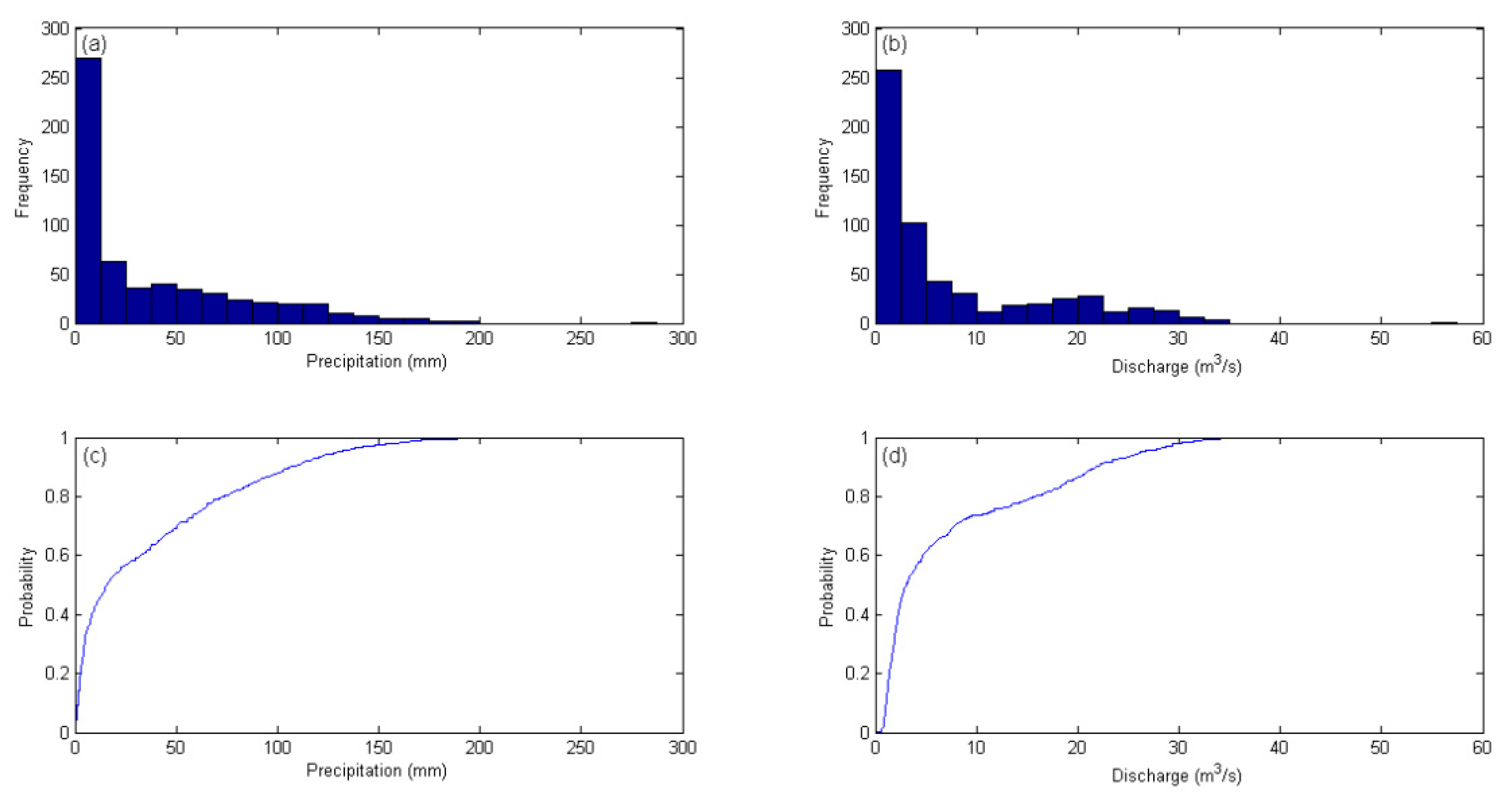
As an initial preanalysis, the stationarity and homogeneity of precipitation and discharge series are also tested through Augmented Dickey-Fuller (ADF) [47] and Levene’s [48] test, respectively. The results show that both the p values of ADF test for precipitation and discharge are far less than 0.001, implying that both of the two series are stationary. In addition, the p values of Levene’s test are 0.28 and 0.14, respectively, larger than the commonly used significance level 0.05, meaning that the samples are homogeneous. To apply Copula formula to the precipitation and discharge data set for the river, we first use the empirical distribution function, that is, Equation (1) to estimate the marginal distribution functions of river discharge and precipitation. The histograms and empirical distribution functions of precipitation and discharge are shown in Figure 4. The empirical distribution function is a pure interpolated method, which limits the range of the random variable between the maximum and minimum of the sample points and, thus, avoids the risk from extrapolation, that is, the points larger than the maximal sample or smaller than the minimal sample will have a very inaccurate estimation. Their copula distribution and density functions are then estimated using Equations (2) and (3). The goodness-of-fit test, that is, the Cramer-von-Mises test [49] was carried out, and the p value is 0.901, which means the nonparametric copula obtained through Equations (2) and (3) can effectively capture the dependence structure of the data.

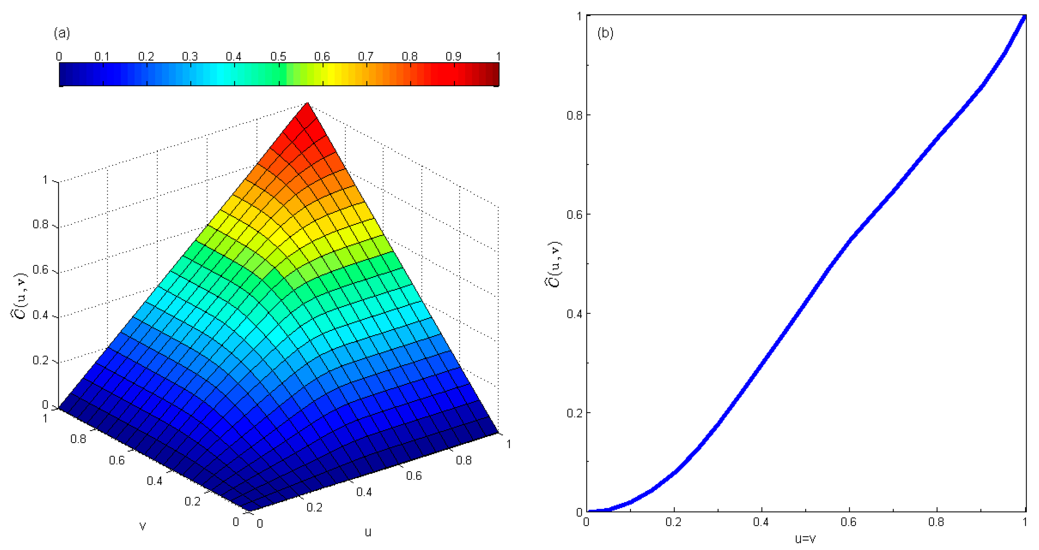
From now on, we use $X$ to represent the river discharge and $Y$ the precipitation. Let $U=F_1(X)$ and $V=F_2(Y)$ be the standardized $X$ and $Y$, respectively. Then, ${\widehat{F}}_1(x)$ and ${\widehat{F}}_2(y)$ denote the empirical distribution of $X$ and $Y$, and ${\widehat{F}}_1^{-1}$ and ${\widehat{F}}_2^{-1}$ represent the inverse functions of ${\widehat{F}}_1(x)$ and ${\widehat{F}}_2(y)$. To apply Equation (2), $n$ is set to be 588, which is the total number of pairs of data. The value of $h$ is set to be 0.12 as suggested by Chen and Huang [43] (that is, it should be on the same order with the value of $n^{-1/3}$). Both the small increments $\Delta u$ and $\Delta v$ in Equation (3) are set to 0.01 to calculate the approximate value of $\widehat{c}(u,v)$ at each point. Figure 5 and Figure 6 display the estimated $\widehat{C}(u,v)$ and $\widehat{c}(u,v)$. As illustrated in Figure 5a, the surface of $\widehat{C}(u,v)$ forms an upward slope with values ranging from 0 to 1 on the region of the unit square, that is, $(u,v)\in {[0,1]}^2$, and with the corner points values: $\widehat{C}(0,0)=0$, $\widehat{C}(0,1)=0$, $\widehat{C}(1,0)=0$, $\widehat{C}(1,1)=1$. The cross-section of $\widehat{C}(u,v)$ in Figure 5b shows a monotonous increasing curve from 0 to 1 in the interval [0,1]. All of these features are consistent with the characteristics of the Copula joint distribution function.

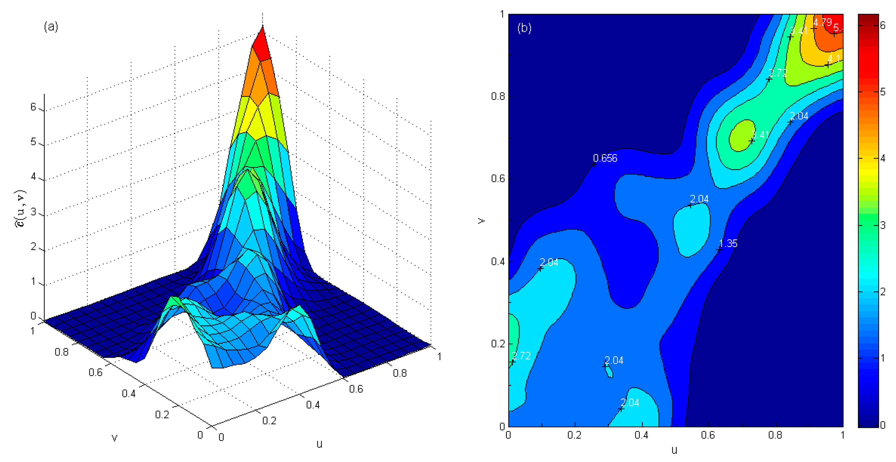
The 3-D plot of estimated Copula density function, $\widehat{c}(u,v)$, is illustrated in Figure 6a over the unit square region ${[0,1]}^2$. Apparently, the joint probability density function of the precipitation and the river discharge is neither a normal nor lognormal distribution. The diagonal region of the function, that is, the place around $u=v$, bulges upward, and the function becomes flat close to zero near the corner points, (0,1) and (1,0). The upraised portion of the surface is not smooth, containing some small pits and hills, and it rises significantly near the corner point (1,1).

The plan view contour map of $\widehat{c}$ is plotted in Figure 6b, which can help us understand Figure 6a from another perspective. From Figure 6b we see that the color is dark blue near the corner points (0,1) and (1,0), which illustrates that the density function is zero near the two corner points. The density function with positive values (that is, the places with light blue, green, yellow and, red) is along the diagonal region, that is, near the line $u=v$. In addition, at the left-bottom region, that is, the region near $u=v$ and $u<0.5$, $v<0.5$, the contours are relatively sparse, and the colors are light blue or green (the values are lower than 2.8). Notice that both the value and the gradient of the density function are small in this area, and the density surface is gentle and flat. On the contrary, at the right-upper region, that is, the area near $u=v$ and $u>0.5$, $v>0.5$, the contour is dense, and the color is up to red (the value reaches 6.2) near the point (1,1). Both the gradient and value are relatively large around this area, and the density surface is steep. The value of density rises sharply with the increase of $u$ and $v$.

The bulging up surface means that there is a high possibility that the pair of $(u,v)$ in these ranges will occur, while the area where $\widehat{c}=0$ suggests that the probability of the concurrence of the pair of $(u,v)$ values in these ranges is small. The fact that the surface $\widehat{c}(u,v)$ is bulging upward along the diagonal and becomes zero around (1,0) and (0,1) rectifies the positive linear correlation between the discharge and precipitation.

On the other hands, the narrow contours and the abrupt uprising of the function around the corner point (1,1) suggest a strong correlation between the upper tails of river discharge and precipitation. In other words, when the precipitation is large, the probability of large discharge can increase dramatically, and the dependence pattern between precipitation and discharge at rainy season is quite different from the pattern of any other seasons.

In contrast, the sparse contours and flat lower tail around (0,0) suggest that correlation between small discharge and precipitation is weak. That is, the probability of small discharge does not necessarily increase even though the precipitation is limited. This result reflects the fact that the precipitation is not the sole source of river discharge. Other sources such as snowmelt and regional groundwater flow may contribute to the river discharge.

In addition, the upper and lower tail dependence coefficients can be quantified through Equations (6) and (7), where ${\widehat{\lambda }}_u$ = 0.58 and ${\widehat{\lambda }}_l$ = 0. The values of the upper and lower coefficients suggest that river discharge is strongly related to heavy rainfall and has little relationship with light rainfall. Although 0.58 is less than 1, it is much larger than zero. This result means that there is a relatively strong relationship between maximum discharge and precipitation, and the dependence between minimum discharge and precipitation is very small. This result is consistent with the analysis in Figure 6a,b, and here the degree of the dependencies are quantified.

4.1.2. Comparison between the Non-Parametric and Parametric Copulas

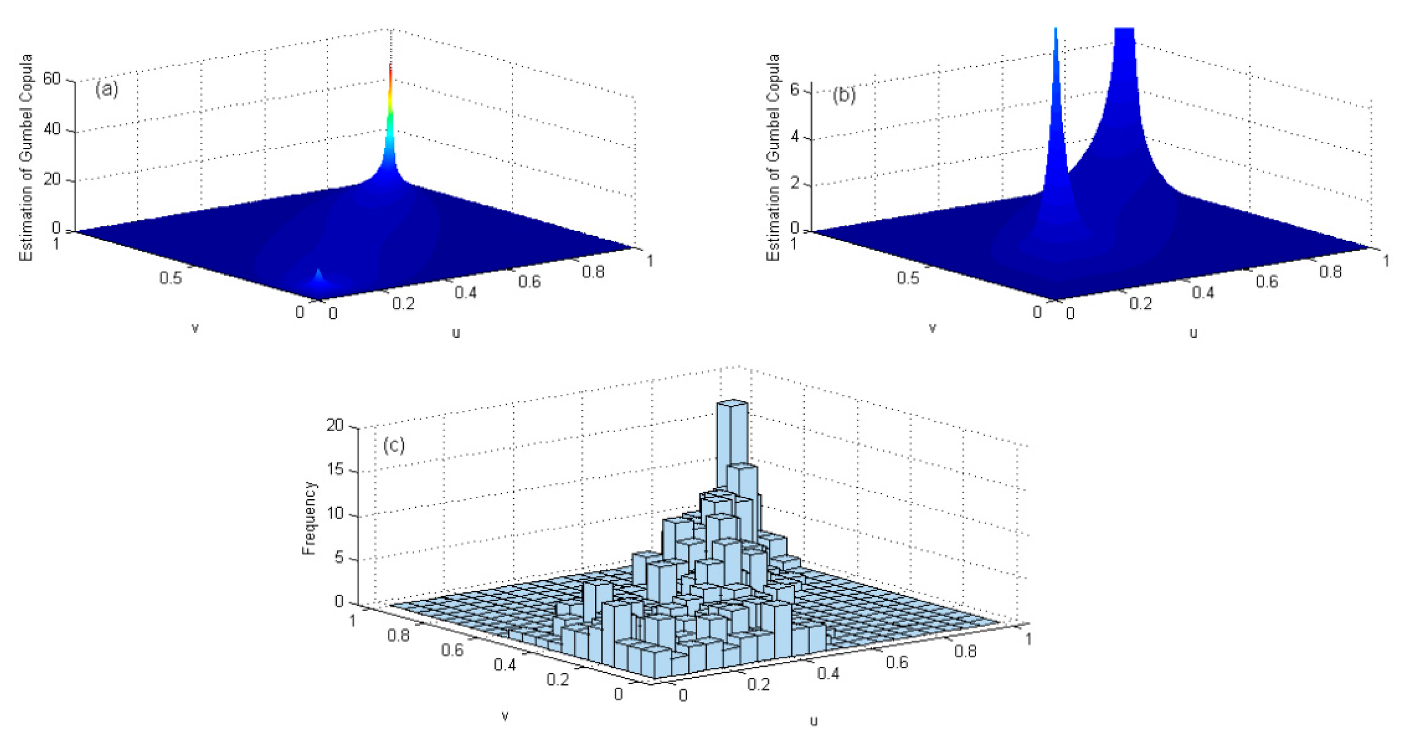
For comparing the performances between parametric and non-parametric Copulas, five usual parametric Copulas, that is, Gaussian, t, Gumbel, Frank, Clayton Copulas are used to fit the standardized Urumqi River’s data. The p values of the above five parametric copulas and the non-parametric copula used in this paper under the Cramer-von-Mises test are shown in

Table 1. The p values of Cramer-von-Mises test between the observation data and various Copula models.

Cramer-von-Mises Test	Non-Parametric Copula	Gaussian Copula	t Copula	Gumbel Copula	Frank Copula	Clayton Copula
p value	0.901	0.250	0.124	0.319	0.179	0.002

. It can be seen that four of the five parametric Copulas that is—Gaussian, t, Gumbel, and Frank—pass the Cramer-von-Mises test in the sense of significance level 0.05 and, thus, can be viewed as fitting well with the data, though their p values are not so much as the non-parametric Copula of this paper, that is, 0.901. Generally speaking, the larger p values imply better fitting results. Therefore, the density surface of the best fitted one of the parametric Copulas with p value 0.319, that is, Gumbel Copula, is drawn in Figure 7. In Figure 7, both panels (a) and (b) are the fitted Gumbel Copula density surfaces but with different vertical axis range, where (a) is between 0 and 60, while (b) is between 0 and 6.5. Panel (c) shows the sample histogram of the standardized discharge and precipitation. Comparing Figure 6a and Figure 7a–c, we can see that the shapes of the non-parametric Copula density surface (Figure 6a) and the sample histogram (Figure 7c) are very close to each other, while both of them have some differences with the Gumbel density surface Figure 7a,b, especially near the point (0,0), where the Gumbel surface cocks upward, while the nonparametric Copulas (Figure 6a) and the histogram (Figure 7c) have no such performances. These phenomena indicate that the non-parametric Copula method can get a better fitting effect in the case of this paper compared with parametric methods.

Of course, in general, the parametric Copula methods have a better ability of extrapolation than non-parametric Copula, when the fitting is indeed accurate [11]. Though this paper does not involve extrapolation problems because the marginal distributions are estimated by the empirical distribution functions.

4.2. Simulation and Validation

4.2.1. Simulation and Analysis

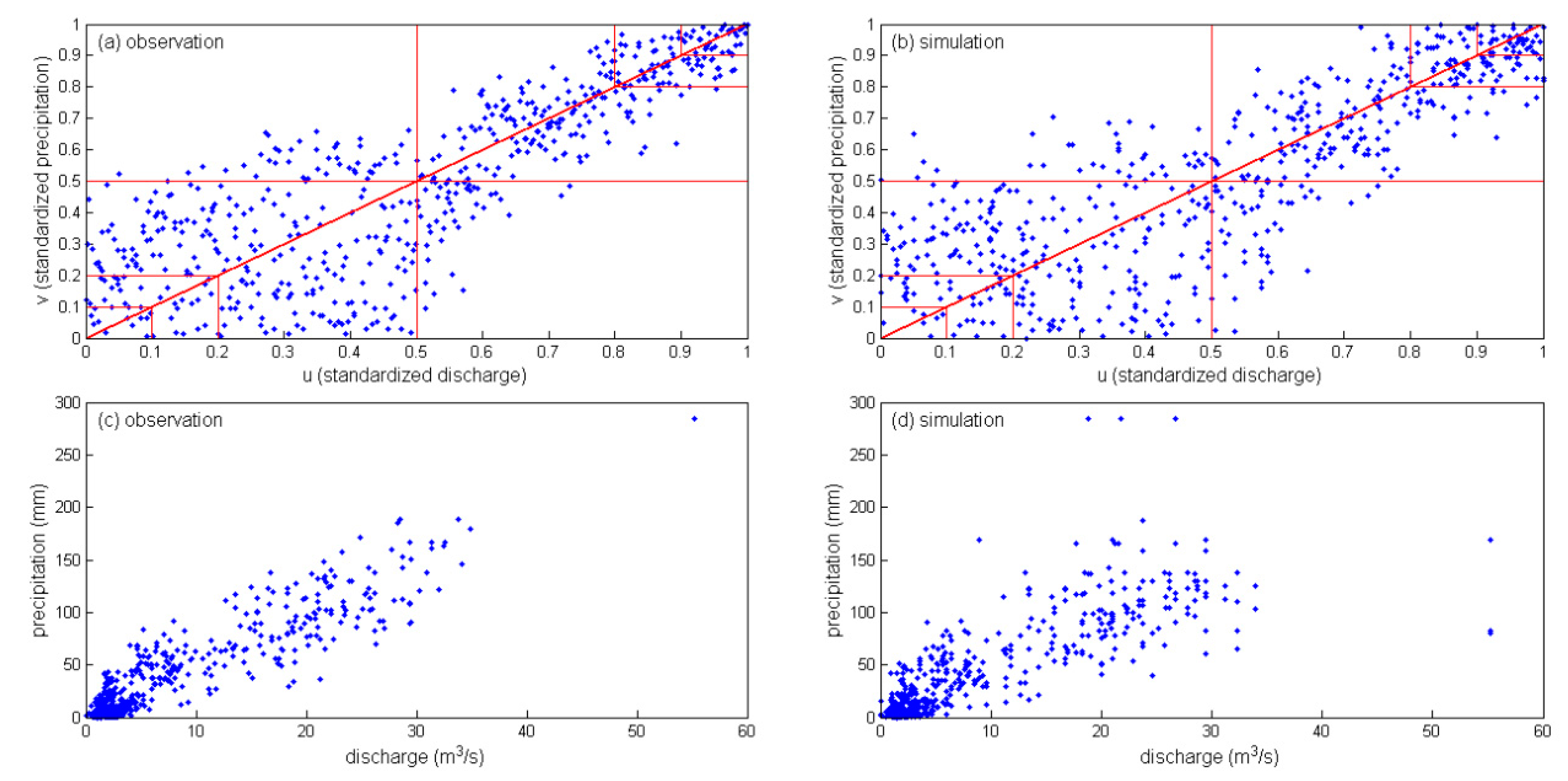
To verify the validity of the estimated surface $\widehat{c}(u,v)$ in Section 4.1, we conduct numerical simulations using $\widehat{c}(u,v)$, which means using $\widehat{c}(u,v)$ as the joint density function and drawing a series of sample points from $\widehat{c}(u,v)$. We then compare this simulated sample points with the actual observation data. The comparisons are shown in Figure 8, where panel (a) is the scatter plot of the 588 standardized real data of precipitation to discharge, panel (b) is the scatter plot with the 588 standardized simulated points, panel (c) is the scatter plot of 588 unstandardized real data, and (d) is the scatter plot with unstandardized simulated points (using ${\widehat{F}}_1^{-1}$ and ${\widehat{F}}_2^{-1}$ to restore each point in (b), then we obtain all the points in (d)).

We analyze Figure 8 regarding the following three aspects, firstly, the shapes of data clusters are very similar between (a) and (b) and between (c) and (d), which indicates that the Copula functions $\widehat{C}(u,v)$ and $\widehat{c}(u,v)$ estimated in this paper are appropriate and correct. The model reflects the relation between precipitation and discharges very well. We further explain the validity of the used model in a quantitative way. In Figure 8a,b, frequency statistics of real observations and simulation points falling in different regions are presented, and some comparisons are also discussed. Because our concern is the extreme values, we mainly focus on the regions of the right-upper and left-bottom regions. They are the regions which are marked by red lines in panels (a) and (b). The results of the frequency statistics are listed in

Table 2. The frequency statistics of observed and simulated data points in different regions.

Frequency	U ≤ 0.1 and V ≤ 0.1	U ≤ 0.2 and V ≤ 0.2	U < 0.5 and V < 0.5	U ≥ 0.9 and V ≥ 0.9	U ≥ 0.8 and V ≥ 0.8	U ≥ 0.5 and V ≥ 0.5
observation	0.0187	0.0748	0.4218	0.0663	0.1718	0.4252
simulation	0.0119	0.0697	0.4065	0.0731	0.1905	0.4473

, where each numerical value is the quotient of the number of points falling into the corresponding region and the total number, that is, 588. According to the table, the simulated frequencies are very close to the real ones in each region, illustrating that the model is reasonable and correct.

Secondly, Figure 8c,d show the unstandardized real and simulated scatter points plots corresponding to (a) and (b). According to (c) and (d), most of the points concentrate at the left-bottom corner, while a small number of points sparsely distribute around the neighborhood of a straight line (is about the line $y=5x$). Apparently, it is hard to recognize the relation between precipitation and discharge through the concentrated data points at the left-bottom of the (c) and (d). However, their relations can be easily seen in (a) and (b). This fact is one of the advantages of the Copula model. The Copula model filters out the marginal distributions of precipitation and discharge respectively, and reveals only the correlation between them.

Thirdly, from panels (a) and (b) and Table 2, most of the points fall in the neighborhood of the diagonal line ($u=v$), while the points are very few at the left-upper and right bottom corners. This result again proves the linear relation between precipitation and discharge. In addition, the frequency of points in the region $U<0.5$ and $V<0.5$ is about 0.4, and the frequency of the region $U\ge 0.5$ and $V\ge 0.5$ is also about 0.4 (as Table 2 shows). However, the points distribute more dispersedly in the region where $U<0.5$ and $V<0.5$, and more intensively in the region and , that means, when $U\ge 0.5$ and $V\ge 0.5$, the points are concentrating along the straight line ($u=v$). This result illustrates that the precipitation has a significant and immediate influence on discharge when precipitation is heavy. However, in the rainless seasons, discharge can be affected by many factors and, thus, the discharge may not immediately decrease even though the precipitation is small. This perhaps is because there is a dynamic balance between river runoff and shallow groundwater. When the river runoff is large, the shallow groundwater is also in saturation, and the larger rainfall will immediately turn into surface runoff to form floodwaters. When the river flow is small, the balance will show that the river water will receive shallow groundwater supply. Research also shows that during the dry season, groundwater recharge accounts for about 30% of the total river volume [50]. In addition, in the dry season, the recharge ratio of the ablation of ice and snow and ablation of frozen soil is also relatively high. Therefore, when precipitation is less, the decline in river flow is not very significant.

4.2.2. Simulation and Analysis with a Large Number of Samples

To ensure the above simulation result is representative, we once again draw 20,000 sample points (that is, more points improve the accuracy and reduce the standard errors) and apply these 20,000 points to estimate the joint probabilities between precipitation and discharge when the precipitation is at heavy or small levels. The corresponding standard errors and 95% confidence intervals are also calculated. The results are shown in

Table 3. The estimated probabilities, standard errors, and 95% confidence intervals of the random vector (X, Y), or (U, V), falling into different regions (X denotes discharge and Y is precipitation, U and V are the standardized X and Y respectively, that is, $U={\widehat{F}}_1(X)$ and $X={\widehat{F}}_1^{-1}(U)$ or $X={\widehat{F}}_1^{-1}(U)$ and $Y={\widehat{F}}_2^{-1}(V)$.

(U, V)	U ≤ 0.1, V ≤ 0.1	U ≤ 0.2, V ≤ 0.2	U < 0.5 V < 0.5	U ≥ 0.9, V ≥ 0.9	U ≥0.8, V ≥ 0.8	U ≥ 0.5, V ≥ 0.5
(X, Y)	X ≤ 1.07, Y ≤ 1.43	X ≤ 1.40, Y ≤ 2.90	X ≤ 3.08, Y ≤ 15.7	X ≥ 21.8, Y ≥ 107.0	X ≥ 15.8, Y ≥ 73.3	X ≥ 3.08, Y ≥ 15.7
Estimated probability	0.018	0.073	0.416	0.058	0.159	0.434
Standard error	0.0009	0.0018	0.0035	0.0017	0.0026	0.0035
95% Confidence interval	(0.0162, 0.0198)	(0.0695, 0.0765)	(0.4091, 0.4229)	(0.0547, 0.0613)	(0.1539, 0.1641)	(0.4271, 0.4409)

, where the $(X,Y)$ denotes the random vector of discharge and precipitation and $(U,V)$ represents the standardized discharge and precipitation, that is, $U={\widehat{F}}_1(X)$ and $V={\widehat{F}}_2(Y)$ or $X={\widehat{F}}_1^{-1}(U)$ and $Y={\widehat{F}}_2^{-1}(V)$. Table 3 means ${\widehat{F}}_1{}^{-1}(0.1)=1.07$, ${\widehat{F}}_2^{-1}(0.1)=1.43$, thus, the probability of ($U<0.1$,$V<0.1$) is equal to the probability of ($X<1.07$,$Y<1.43$) and estimated as 0.018, whose standard error and 95% confidence interval are 0.0009 and (0.0162, 0.0198) and so on.

Table 3 shows that all of the standard errors are less than 0.005, implying the fitting of the 20,000 points is quite accurate. Based on the estimated probabilities in Table 3, P($U<0.1$,$V<0.1$) = 0.018 is much less than P($U\ge 0.9$,$V\ge 0.9$) = 0.058. P($U<0.2$,$V<0.2$) = 0.073 also lower than P($U\ge 0.8$,$V\ge 0.8$) = 0.159. This result suggests that the random points are more likely to fall in the upper-right corner than the lower-left corner. In other words, the relationship between heavy rain and large discharge is closely related, while dry weather will not lead to an immediate small discharge at the same time. These results again agree with the conclusions obtained in Section 4.1.

4.3. Estimation of Conditional Probabilities

Besides the above analysis, the conditional probability values of $X$ in any region given $Y$ can also be calculated through the $\widehat{C}(u,v)$, $\widehat{c}(u,v)$, ${\widehat{F}}_1(·)$, and ${\widehat{F}}_2(·)$. Typical applications of this function address the concern of the probability of maximum discharge occurs when the precipitation exceeds a certain level, or the probability of minimum discharge as the precipitation is less than some certain level. The assessment of these probabilities could guide decision makers or disaster relief groups to make some advanced preparations.

To illustrate this conditional probability analysis, we consider the upper and lower 5% sample quantiles of the Urumqi River discharge as the thresholds of maximum and minimum discharge respectively. We then calculate the corresponding conditional probabilities through Equations (8) and (9). After calculations, let $x_f$ = 26.2 m³/s be the threshold of maximum discharge, and $x_d$ = 0.923 m³/s be the threshold of minimum discharge. The results are listed in

Table 4. The conditional probability that $P(X>x_f|Y>y)$ at $y=$ 73.16, 79.46, 86.30, …, 159.56 mm.

V	0.80	0.82	0.84	0.86	0.88	0.90	0.92	0.94	0.96	0.98
y (mm)	73.16	79.46	86.30	91.97	100.05	105.47	114.98	123.75	137.39	159.56
P	0.23	0.25	0.26	0.28	0.31	0.33	0.36	0.40	0.47	0.64

and

Table 5. The conditional probability that $P(X<x_d|Y<y)$ at $y=$ 0.40, 0.55, 0.90, 1.20, …, 2.90 mm.

V	0.02	0.04	0.06	0.08	0.10	0.12	0.14	0.16	0.18	0.20
y (mm)	0.40	0.55	0.90	1.20	1.40	1.70	1.90	2.10	2.40	2.90
P	0.04	0.08	0.09	0.10	0.11	0.11	0.11	0.11	0.12	0.12

and illustrated in Figure 9. In Table 4, $v=0.8,0.82,\dots ,0.98$ and is calculated by ${\widehat{F}}_2^{-1}$, the inverse function of ${\widehat{F}}_2$ The probabilities are then obtained from Equation (8).

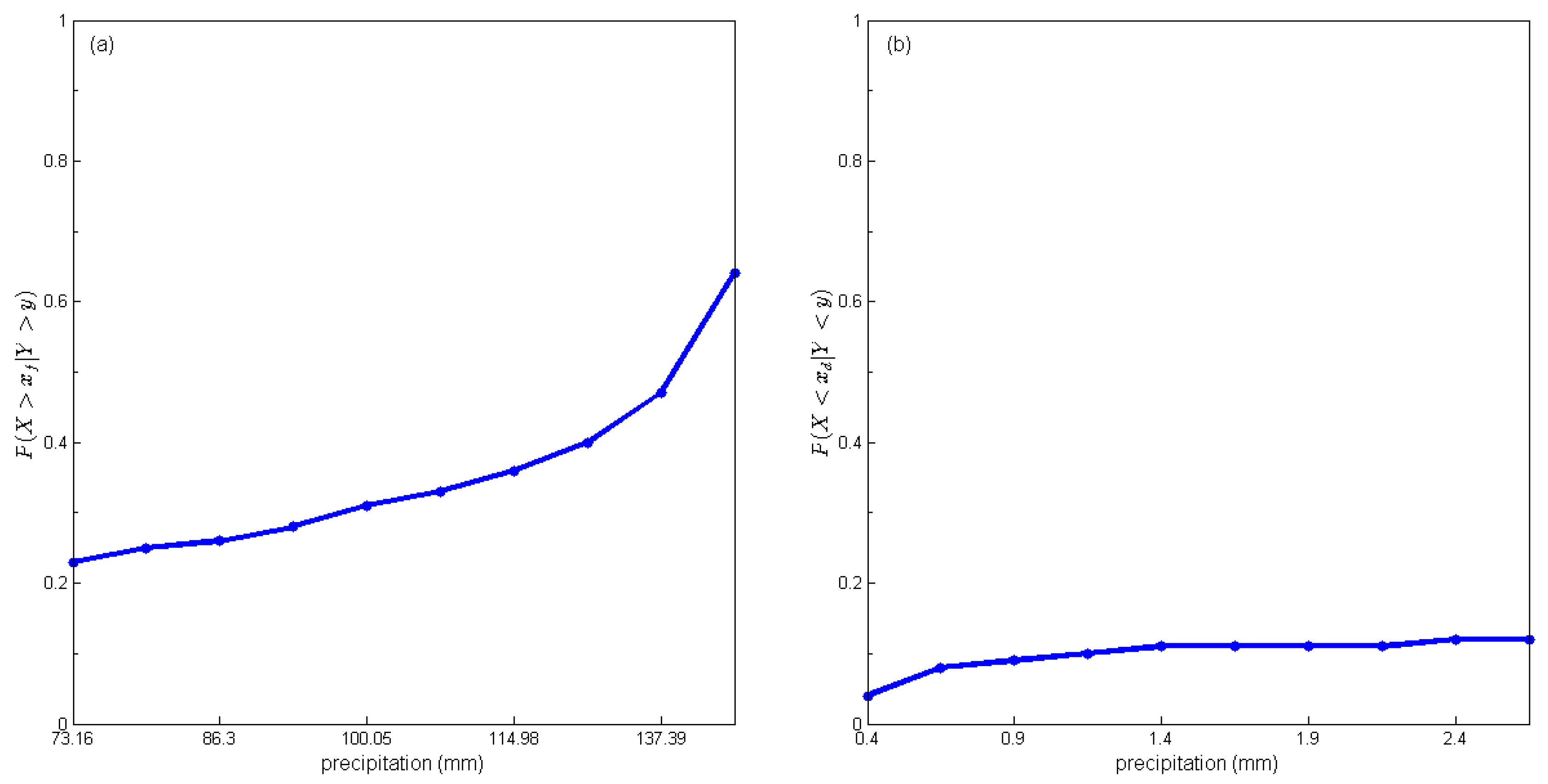
Table 4 shows that the probability of large discharge is 0.23 under the condition that the precipitation is larger than 73.16 mm. This probability becomes 0.25 when the precipitation is larger than 79.46 mm and so on. The probability of large discharge continues to grow with the increasing precipitation. As the precipitation becomes larger than 159.56 mm, the probability of large discharge reaches up to 0.64.

Figure 9a displays the monotonous rising trend of large discharge probability along with the increasing precipitation, and the curve line is concave which means the growth rate is also growing. The rapid growing conditional probability of large discharge once again verifies the strong upper tail correlation discussed in the Section 4.1 and Section 4.2. As a result, preparation of mitigating hazard of large discharge or even flood is necessary since the probability of large discharge is extremely high.

On the contrary, Table 5 and Figure 9b display the conditional probabilities of small discharge when the precipitation is less than the given levels. In Table 5, $v=0.02,0.04,\dots ,0.2$ and is also calculated via ${\widehat{F}}_2^{-1}$. The probabilities are obtained from Equation (9). Table 5 reveals that the probability of small discharge is just 0.04 when the precipitation is lower than 0.4 mm, and the small discharge probability is 0.08 when the precipitation is less than 0.55 mm and so on. Apparently, all the probability values in Table 5 are small and even less than 0.15. This result indicates that the probability of small discharge is not significant even though the precipitation is low. This finding corroborates the conclusion in Section 4.1 and Section 4.2 that the lower tail correlation is small and nearly close to none. The small probabilities in Table 5 suggest that the precipitation is not the decisive factor for minimum discharge.

5. Summary and Conclusions

This paper quantifies the relationship between the Urumqi River’s discharge and precipitation by a nonparametric Copula method. The estimated Copula distribution and density functions, that is, $\widehat{C}(u,v)$ and $\widehat{c}(u,v)$, especially the joint density function, clearly reveal the joint relationship between river discharge and precipitation regardless of their respective marginal distributions. The bulging part of the joint density function around the diagonal region, that is, the region near $u=v$, again verifies the strong linear correlation between rainfall and river discharge, which has already been proved by correlation coefficient 0.919 in Section 2.2. On the other hands, the highly bulged upper corner and the narrow contour lines near the point (1,1) imply a strong upper tail correlation. That is, the possibility of the concurrence of the large river discharge and heavy precipitation is extremely high. Additionally, $\widehat{c}(u,v)$ is flat at the lower tail, that is, the region near the point (0,0). This behavior demonstrates that the possibility of the concurrence of the minimum river discharge and low precipitation is low. In other words, light precipitation does not directly correlate with river discharge at low values. Physically, light precipitation likely immediately infiltrates into the subsurface or evaporates back to the atmosphere or produces limited surface runoff, which is retained by surface depressions and ultimately infiltrates into the subsurface or is evaporated. The coefficients of tail dependence quantify the dependence of upper and lower tails (that is, extreme events).

The simulation through the estimated surface $\widehat{c}(u,v)$ are conducted and the observed data and simulation results are compared to verify the rationality of the model $\widehat{c}(u,v)$. The comparisons prove the model. Furthermore, we use the model $\widehat{c}(u,v)$ to simulate 20,000 points to estimate the joint probability of discharge and precipitation. The analysis of the results further demonstrates that the joint probability of maximum discharge and precipitation is large while the joint probability of minimum discharge and precipitation is small. This result further verifies the conclusion that the upper tail dependence between discharge and precipitation is strong while the lower tail dependence is weak.

The conditional probability of maximum and minimum discharge for this study area under the different precipitation levels are calculated through the estimated joint probability distribution function. The analysis shows that the probability of large discharge can substantially increase with the increase in the precipitation. Specifically, as the precipitation becomes larger than 159.56 mm, the probability of large discharge reaches 0.64. With this level of precipitation, the analysis recommends an advanced warning of maximum discharge. On the contrary, the probability of small discharge does not increase with the decrease of the precipitation (that is, the probabilities are less than 0.15). In particular, when the precipitation is less than 0.4, the probability of small discharge is only 0.04. Therefore, we are certain that the precipitation is not the only water source for the Urumqi River during the rainless seasons. The groundwater and snowmelt from Tianshan Mountain and other factors likely sustain the flow of the Urumqi River. Further, for the study area, precipitation can be used to predict floods during rainy seasons, but it is not suitable for forecasting drought during rainless seasons.

Because of the importance of Urumqi River in the local area, the results of this study have practical implications for analyzing maximum and minimum discharge in the area. In addition, this paper introduces a new nonparametric estimation approach for Copula function in statistics to the field of hydrometeorology. This paper demonstrates the practical aspects of this method through the analysis of the relationship of Urumqi River’s discharge and precipitation. The methodology and results of this study can be tried to be used in other areas for other issues in the hydrometeorological field.

References

- Vörösmarty, C.J.; Green, P.; Salisbury, J.; Lammers, R.B. Global water resources: Vulnerability from climate change and population growth. Science 2000, 289, 284–288. [Google Scholar] [CrossRef] [PubMed]
- Chen, Y.; Xu, C.; Yang, Y.; Hao, X.; Shen, Y. Hydrology and water Resources variation and its responses to regional climate change in Xinjiang. J. Geogr. Sci. 2010, 20, 599–612. [Google Scholar]
- Oki, T.; Kanae, S. Global hydrological cycles and world water resources. Science 2006, 313, 1068–1072. [Google Scholar] [CrossRef] [PubMed]
- Jiang, Y.; Zhou, C.; Cheng, W. Streamflow trends and hydrological response to climatic change in Tarim headwater basin. J. Geogr. Sci. 2007, 17, 51–61. [Google Scholar] [CrossRef]
- Kong, Y.; Pang, Z. What is the primary factor controlling trend of Glacier No. 1 runoff in the Tianshan Mountains: Temperature or precipitation change? Hydrol. Res. 2017, 48, 231–239. [Google Scholar] [CrossRef]
- Li, Z.; Wang, W.; Zhang, M.; Wang, F.; Li, H. Observed changes in streamflow at the headwaters of the Ürümqi River, eastern Tianshan, central Asia. Hydrol. Process. 2010, 24, 217–224. [Google Scholar] [CrossRef]
- Liu, Y.; Huo, X.; Liu, Y.; Hao, Y.; Fan, Y.; Zhong, Y.; Yeh, T.J. Analyzing monthly average streamflow extremes in the upper Ürümqi River based on a GPD model. Environ. Earth Sci. 2015, 74, 4885–4895. [Google Scholar] [CrossRef]
- Liu, Y.; Wu, J.; Liu, Y.; Hu, B.X.; Hao, Y.; Huo, X.; Fan, Y.; Yeh, T.J.; Wang, Z.-L. Analyzing effects of climate change on streamflow in a glacier mountain catchment using an ARMA model. Quat. Int. 2015, 358, 137–145. [Google Scholar] [CrossRef]
- Sorg, A.; Bolch, T.; Stoffel, M.; Solomina, O.; Beniston, M. Climate change impacts on glaciers and runoff in Tien Shan (Central Asia). Nat. Clim. Chang. 2012, 2, 725–731. [Google Scholar] [CrossRef]
- Xu, J.; Chen, Y.; Lu, F.; Li, W.; Zhang, L.; Hong, Y. The nonlinear trend of runoff and its response to climate change in the Aksu River, western China. Int. J. Clim. 2011, 31, 687–695. [Google Scholar] [CrossRef]
- Sklar, M. Fonctions de Répartition À N Dimensions Et Leurs Marges; Université Paris: Saint-Denis, France, 1959; Volume 8, pp. 229–231. [Google Scholar]
- De Michele, C.; Salvadori, G. A Generalized Pareto intensity-duration model of storm rainfall exploiting 2-Copulas. J. Geophys. Res.-Atmos. 2003, 108. [Google Scholar] [CrossRef] [Green Version]
- Dupuis, D.J. Using copulas in hydrology: Benefits, cautions, and issues. J. Hydrol. Eng. 2007, 12, 381–393. [Google Scholar] [CrossRef]
- Favre, A.-C.; EI Adlouni, S.; Perreault, L.; Thiemonge, N.; Bobee, B. Multivariate hydrological frequency analysis using copulas. Water Resour. Res. 2004, 40, W01101. [Google Scholar] [CrossRef]
- Salvadori, G.; De Michele, C. On the use of copulas in hydrology: Theory and practice. J. Hydrol. Eng. 2007, 12, 369–380. [Google Scholar] [CrossRef]
- Salvadori, G.; De Michele, C.; Kottegoda, N.T.; Rosso, R. Extremes in Nature: An Approach Using Copulas; Springer: Dordrecht, The Netherlands, 2007; p. 292. [Google Scholar]
- Kao, S.-C.; Govindaraju, R.S. A copula-based joint deficit index for droughts. J. Hydrol. 2010, 380, 121–134. [Google Scholar] [CrossRef]
- Lee, T.; Modarres, R.; Ouarda, T.B.M.J. Data-based analysis of bivariate copula tail dependence for drought duration and severity. Hydrol. Process. 2013, 27, 1454–1463. [Google Scholar] [CrossRef]
- Liu, C.-L.; Zhang, Q.; Singh, V.P.; Cui, Y. Copula-based evaluations of drought variations in Guangdong, South China. Nat. Hazards 2011, 59, 1533–1546. [Google Scholar] [CrossRef]
- Ma, M.; Song, S.; Ren, L.; Jiang, S.; Song, J. Multivariate drought characteristics using trivariate Gaussian and Student t copulas. Hydrol. Process. 2013, 27, 1175–1190. [Google Scholar] [CrossRef]
- Janga Reddy, M.; Ganguli, P. Application of copulas for derivation of drought severity-duration-frequency curves. Hydrol. Process. 2012, 26, 1672–1685. [Google Scholar] [CrossRef]
- Wong, G.; van Lanen, H.A.J.; Torfs, P.J.J.F. Probabilistic analysis of hydrological drought characteristics using meteorological drought. Hydrol. Sci. J. 2013, 58, 253–270. [Google Scholar] [CrossRef] [Green Version]
- Ariff, N.M.; Jemain, A.A.; Ibrahim, K.; Wan Zin, W.Z. IDF relationships using bivariate copula for storm events in Peninsular Malaysia. J. Hydrol. 2012, 470–471, 158–171. [Google Scholar] [CrossRef]
- Balistrocchi, M.; Bacchi, B. Modelling the statistical dependence of rainfall event variables through copula functions. Hydrol. Earth Syst. Sci. 2011, 15, 1959–1977. [Google Scholar] [CrossRef] [Green Version]
- Gargouri-Ellouze, E.; Chebchoub, A. Modelling the dependence structure of rainfall depth and duration by Gumbel’s copula. Hydrol. Sci. J. 2008, 53, 802–817. [Google Scholar] [CrossRef]
- Ghosh, S. Modelling bivariate rainfall distribution and generating bivariate correlated rainfall data in neighbouring meteorological subdivisions using copula. Hydrol. Process. 2010, 24, 3558–3567. [Google Scholar] [CrossRef]
- Singh, V.P.; Zhang, L. IDF curves using the Frank Archimedean copula. J. Hydrol. Eng. 2007, 12, 651–662. [Google Scholar] [CrossRef]
- Vandenberghe, S.; Verhoest, N.E.C.; De Baets, B. Fitting bivariate copulas to the dependence structure between storm characteristics: A detailed analysis based on 105 year 10 min rainfall. Water Resour. Res. 2010, 46. [Google Scholar] [CrossRef] [Green Version]
- Zhang, L.; Singh, V.P. Bivariate rainfall frequency distributions using archimedean copulas. J. Hydrol. 2007, 332, 93–109. [Google Scholar] [CrossRef]
- Grimaldi, S.; Serinaldi, F.; Napolitano, F.; Ubertini, L. A 3-copula function application for design hyetograph analysis. In Proceedings of the Symposium S2, the Seventh IAHS Scientific Assembly, Foz do Iguaçu, Brazil, 3–9 April 2015; Volume 293, pp. 203–211. [Google Scholar]
- Bezak, N.; Mikoš, M.; Šraj, M. Trivariate frequency analyses of peak discharge, hydrograph volume and suspended sediment concentration data using copulas. Water Resour. Manag. 2014, 28, 2195–2212. [Google Scholar] [CrossRef]
- Chen, L.; Singh, V.P.; Guo, S.L.; Hao, Z.C.; Li, T.Y. Flood Coincidence Risk Analysis Using Multivariate Copula Functions. J. Hydrol. Eng. 2012, 17, 742–755. [Google Scholar] [CrossRef]
- Karmakar, S.; Simonovic, S.P. Bivariate flood frequency analysis. Part 2: A copula-based approach with mixed marginal distributions. J. Flood Risk Manag. 2009, 2, 32–44. [Google Scholar] [CrossRef]
- Renard, B.; Lang, M. Use of a gaussian copula for multivariate extreme value analysis: Some case studies in hydrology. Adv. Water Resour. 2007, 30, 897–912. [Google Scholar] [CrossRef]
- Sraj, M.; Bezak, N.; Brilly, M. Bivariate flood frequency analysis using the copula function: A case study of the Litija station on the Sava River. Hydrol. Process. 2015, 29, 225–238. [Google Scholar] [CrossRef]
- Serinaldi, F.; Grimaldi, S.; Napolitano, F.; Ubertini, L. A 3-Copula function application to flood frequency analysis. In Proceedings of the IASTED International Conference Environmental Modelling and Simulation, St. Thomas, Virgin Islands, USA, 22–24 November 2004; pp. 202–206. [Google Scholar]
- Grimaldi, S.; Serinaldi, F. Asymmetric copula in multivariate flood frequency analysis. Adv. Water Resour. 2006, 29, 1155–1167. [Google Scholar] [CrossRef]
- Zhang, J. Analysis on flood frequency of Urumqi River. Arid Land Geogr. 1997, 20, 1–10. [Google Scholar]
- De Michele, C.; Salvadori, G.; Canossi, M.; Petaccia, A.; Rosso, R. Bivariate statistical approach to check adequacy of dam spillway. J. Hydrol. Eng. 2005, 10, 50–57. [Google Scholar] [CrossRef]
- Deheuvels, P. La fonction de d′ependance empirique et ses propri′et′es. Un test non param′erique d’ind′ependance. Acad. R. Belg. Bull. Cl. Sci. 1979, 65, 274–292. [Google Scholar]
- Lejeune, M.; Sarda, P. Smooth estimators of distribution and density functions. Comput. Stat. Data Anal. 1992, 14, 457–471. [Google Scholar] [CrossRef]
- Fermanian, J.D.; Scaillet, O. Nonparametric estimation of copulas for time series. J. Risk 2003, 5, 25–54. [Google Scholar] [CrossRef] [Green Version]
- Chen, S.; Huang, T.M. Nonparametric estimation of copula functions for dependence modeling. Can. J. Stat. 2007, 35, 265–282. [Google Scholar] [CrossRef]
- Gao, M.; Han, T.; Ye, B.; Jiao, K. Characteristics of melt water discharge in the Glacier No. 1 basin, headwater of Urumqi River. J. Hydrol. 2013, 489, 180–188. [Google Scholar]
- Liu, Y.; Lu, M.; Huo, X.; Hao, Y.; Liu, Y.; Fan, Y.; Cui, Y.; Metivier, F. A Bayesian analysis of Generalized Pareto Distribution of runoff minima. Hydrol. Process. 2016, 30, 424–432. [Google Scholar] [CrossRef]
- Liu, Y. Study on Mass Transport and Hydraulics of Gravel Bed Stream in a High Mountain, the Urumqi River (Chinese Tianshan). Doctoral Dissertation, Institut de Physique du Globe de Paris, Paris, France, 2008. [Google Scholar]
- Fuller, W.A. Introduction to Statistical Time Series; John Wiley and Sons: New York, NY, USA, 1976. [Google Scholar]
- Levene, H. Robust tests for equality of variances. In Contributions to Probability and Statistics. Essays in Honor of Harold Hotelling; Stanford University Press: Palo Alto, CA, USA, 1960; pp. 279–292. [Google Scholar]
- Cramér, H. On the Composition of Elementary Errors: First paper: Mathematical deductions. Scand. Actuar. J. 1928, 1928, 13–74. [Google Scholar] [CrossRef]
- Sun, C.; Chen, Y.; Li, W.; Li, X.; Yang, Y. Isotopic time series partitioning of streamflow components under regional climate change in the Urumqi River, northwest China. Hydrol. Sci. J. 2016, 61, 1443–1459. [Google Scholar] [CrossRef]
Figure 1.
The DEM map and hydrometeorological observation sites in the upstream of Urumqi River basin.
Figure 2.
The monthly average precipitation and discharge series of Urumqi River from 1958 to 2006. The panel (a) is the precipitation sequence and panel (b) is the discharge sequence.
Figure 3.
The boxplots of precipitation and discharge for each month and their autocorrelation functions with lags 1 to 20. (a) Boxplot of precipitation, (b) boxplot of discharge, (c) autocorrelation function of precipitation, (d) autocorrelation function of discharge.
Figure 4.
The histograms and empirical distribution functions of the samples of precipitation and discharge. (a) histogram of precipitation, (b) histogram of discharge, (c) empirical distribution function of precipitation, (d) empirical distribution function of discharge.
Figure 5.
The estimations of Copula distribution function between river discharge and precipitation. denotes the standardized river discharge and is the standardized precipitation. The panel (a) is the distribution function and panel (b) is the cross-section of at .
Figure 6.
The estimations of Copula density function between river discharge and precipitation. denote the standardized river discharge and is the standardized precipitation. The panel (a) is the density function , and panel (b) is the contour map of .
Figure 7.
The fitted Gumbel density surface and the histogram of the standardized discharge-precipitation pairs. (a) The Gumbel density surface with vertical axis range 0 to 60, (b) the Gumbel density surface with vertical axis range 0 to 6.5, (c) the histogram of the sample pairs after standardization.
Figure 8.
The observation and simulation data points between precipitation and discharge before and after standardization. denotes the standardized discharge and is the standardized precipitation. The panels (a,b) are the scatter diagrams of observed and simulated discharge and precipitation after standardization and the panels (c,d) are the scatter diagrams of observed and simulated discharge and precipitation without standardization.
Figure 9.
The conditional probabilities of large and small discharge at different precipitation levels. (a) conditional probabilities of large discharge, (b) conditional probabilities of small discharge