Nonstationary Flood Frequency Analysis Using Univariate and Bivariate Time-Varying Models Based on GAMLSS

Abstract

With the changing environment, a number of researches have revealed that the assumption of stationarity of flood sequences is questionable. In this paper, we established univariate and bivariate models to investigate nonstationary flood frequency with distribution parameters changing over time. Flood peak Q and one-day flood volume W₁ of the Wangkuai Reservoir catchment were used as basic data. In the univariate model, the log-normal distribution performed best and tended to describe the nonstationarity in both flood peak and volume sequences reasonably well. In the bivariate model, the optimal log-normal distributions were taken as marginal distributions, and copula functions were addressed to construct the dependence structure of Q and W₁. The results showed that the Gumbel-Hougaard copula offered the best joint distribution. The most likely events had an undulating behavior similar to the univariate models, and the combination values of flood peak and volume under the same OR-joint and AND-joint exceedance probability both displayed a decreasing trend. Before 1970, the most likely combination values considering the variation of distribution parameters over time were larger than fixed parameters (stationary), while it became the opposite after 1980. The results highlight the necessity of nonstationary flood frequency analysis.

1. Introduction

Flood frequency analysis is the premise and foundation of water conservancy project planning and construction. The current flood frequency analysis methods usually assume that the flood series satisfies consistency, that is, that the distribution form or the statistical law of the flood sequence is fixed [1]. However, with climate change and intensification of human activities, especially the construction of large-scale water conservancy and water conservation engineering and the urbanization process, the runoff yield and concentration mechanism, and the temporal and spatial distribution of flooding have been changed [2]. This results in the inconsistency of flood series and the unreliability of the frequency obtained from current frequency analysis methods [3]. Therefore, it is of great significance to study the nonstationary flood frequency analysis methods [4].

Existing nonstationary flood frequency analysis methods in literature include mixture distribution methods, conditional probability distribution methods, and time-varying moment methods. The main idea of the nonstationary flood frequency analysis methods based on mixture distribution is that the individuals of the extreme series are not from the same population [5]. That is, the series formed by different hydrological processes does not follow the same distribution, thus it was assumed to consist of several sub-distributions. The nonstationary flood frequency analysis methods based on conditional probability distribution divide the flood into several periods based on the differences in flood formation mechanism, analyze the occurrence probability of annual maximum value in the different periods, and then obtain the probability density function of the extreme series [6].

Different from the mixture distribution models and conditional probability distribution models, models with time-varying moment consider the change of climate and land surface to have resulted in a change in the physical processes and mechanism of flood generation, such that the parameters of the distribution followed by the flood sequence are functions of time rather than constant. Much attention has been paid to time-varying moment models [7]. Vasiliades et al. [8] applied a time-varying moment model based on Generalized Extreme Value (GEV) distribution to analyze nonstationary frequency, through assuming the parameters of GVE distribution to be the functions of time or other factors and conducting a goodness-of-fit test to the model, thus verifying the significance of the nonstationarity of hydrological sequences.

This study addressed models with time as covariate for nonstationary flood frequency analysis based on GAMLSS (Generalized Additive Models for Location, Scale, and Shape) theory. GAMLSS was first proposed by Rigby and Stasinopoulos [9,10]. This model overcomes the limitations of the GLM and GAM models, greatly expands the range of the distribution types, and provides a variety of ways to produce different distributions, including a series of continuous and discrete distributions with high skewness and/or high peak. In addition, the systematic components provide more plentiful content. For example, it can introduce more complex parametric (linear or non-linear), semi parametric, non-parametric, or random-effect terms to establish models between the distribution parameters (mean, variance, etc.) and the explanatory variables. The GAMLSS model has been widely applied in the military, economics, medicine, and other fields [11,12,13]. Hydrologists have also done many researches using GAMLSS in recent years. Serinaldi and Kilsby [14] used the GAMLSS model to analyze the monthly rainfall data of 6 stations in England and Wales. They found that the model could better describe the characteristics of rainfall series, and had better performance for fitting the relation between extreme rainfall events, rainfall and atmospheric circulation index, and sea surface temperature. López and Francés [15] proposed two methods based on the GAMLSS model to investigate the nonstationary frequency analysis of the annual maximum flood records of 20 Spanish inland rivers. The results illustrate that the nonstationarity of flood series caused by the effects of climate change and human activities can not to be ignored, and GAMLSS provides a convenient and flexible model framework for considering the influence of climate factors and human activities in the analysis of non-stationary flood frequency.

In flood frequency analysis, univariate probability distribution functions are usually used to estimate the occurrence probability or magnitude of the flood peak or volume in a certain region. However, flood events involve more than one characteristic variable such as flood peak discharge, flood volume, flood water level, etc. In order to estimate the probability of flooding, one needs to know not only the high and extreme values of each variable, but also the likelihood of their occurring simultaneously [16]. The main issue of the univariate models is their difficulties in capturing the underlying joint probability among multiple physical processes, and this will lead to underestimation of the associated occurring probability [17]. For instance, if only the rainfall is considered to estimate the flood risk for a catchment, the resultant estimation would be significantly lower than its true risk, when there is a statistically significant dependence between the rainfall on the catchment and the downstream high water levels. To this end, bivariate models are used to address this issue [18].

Copula functions, for which the marginal distribution of each variable is uniform, were adopted in the bivariate model with time as covariate in this study. They are popular in high-dimensional statistical applications because they allow one to easily model and estimate the distribution of random vectors by estimating marginals and copulae separately. They can describe the linear, non-linear, symmetric, and asymmetric relations between variables, and are simple, flexible, and adaptable in application. Therefore, copulas are effective mathematical tools to construct the multivariate joint distribution and correlation between variables. In recent years, they have been widely used in multivariate hydrological frequency analysis. In drought characteristics analysis, Mirabbasi et al. [19] used a copula function to establish the joint probability distribution between drought duration and drought degree. In rainfall frequency analysis, Zhang and Singh [20] adopted copula functions to construct the bivariate joint distribution between rainfall intensity and depth, rainfall intensity and duration, and rainfall depth and duration, respectively. The results were compared with a Gumbel mixture model and a two-dimensional normal transformation distribution model. Fu G. and Butler D. [21] used the copula method to separate the dependence structure of rainfall variables from their marginal distributions, and analyzed the different impacts of dependence structure and marginal distributions on system performance.

This paper takes Wangkuai Reservoir, which is undergoing substantial change in climate, land use/land cover, and increased number of soil-water conservation projects in Daqing River Basin, to construct both univariate and bivariate time-varying moment models for flood frequency analysis based on GAMLSS theory. The inflow flood peak and flood volume time series (1956–2004) of Wangkuai Reservoir were selected as basic data to discuss the nonstationary univariate and peak-volume bivariate joint flood frequency analysis methods. Flood quantiles and the combined values of flood peak and flood volume under certain exceedance probabilities have been worked out. This study aims to provide new ideas and approaches for nonstationary flood frequency analysis method under a changing environment.

2. Study Region and Data

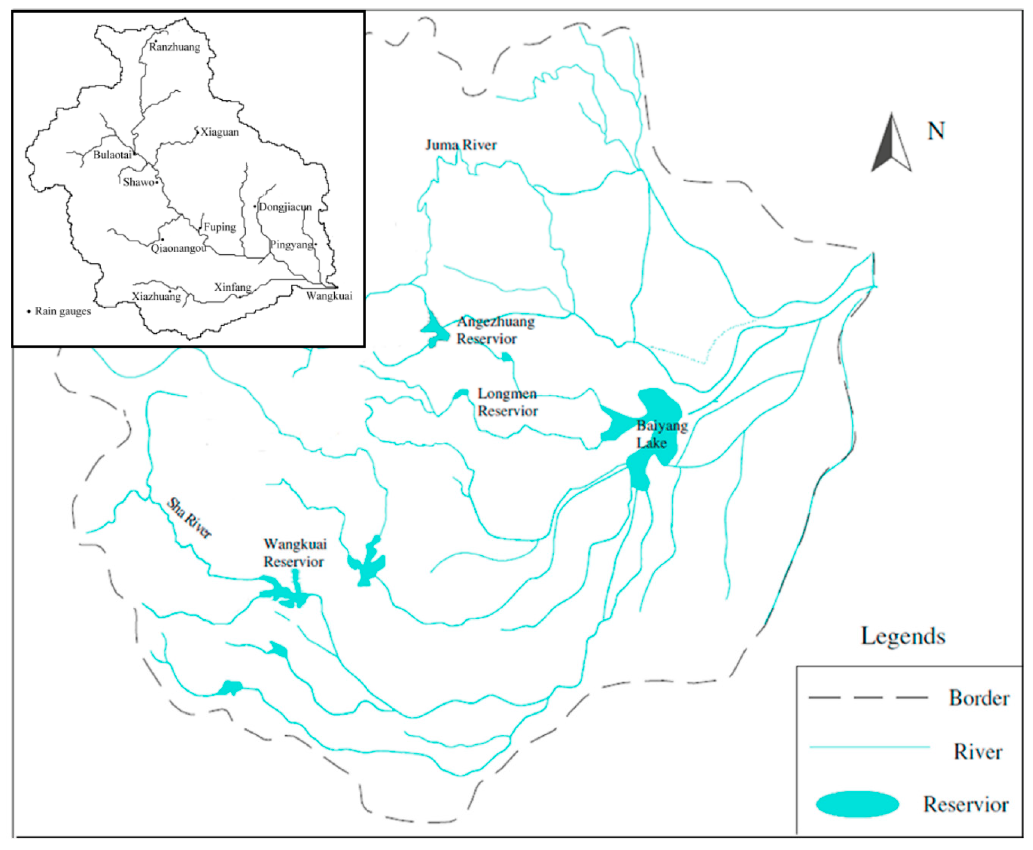
Wangkuai Reservoir is located in the upstream of Sha River, Daqinghe Catchment (Figure 1). Its construction started in June 1958 and finished in September 1960. The control area of the reservoir is 3770 km², and the storage capacity is 13.89 × 10⁸ m³. The currently used design floods were calculated with flood data series under the assumption of stationarity. The watershed receives an average precipitation of 626.4 mm annually, mostly in the summer (70–80%). The annual mean temperature is 7.4 °C.

Since 1980, a series of water conservation measures have been carried out in the Wangkuai Reservoir catchment, such as closing land for reforestation and returning farmland to forest. Meanwhile, a number of small hydraulic structures have been constructed. These factors have increased the vegetation coverage rate and significantly changed the land surface, which has affected the flood process in this watershed and thus resulted in nonstationarity of flood series, as revealed by many studies [22,23,24].

Flooding runoff data have been monitored for a period of 49 years from 1956 to 2004, and collected on hourly basis. The data were provided by Hydrology and Water Resources Survey Bureau of Hebei Province. Maximum flood peak Q and maximum one-day flood volume W₁ of each year are selected in this work.

3. Methods

3.1. Generalized Additive Models in Location, Scale, and Shape (GAMLSS)

In this study, we adopted a general class of regression models which was called the Generalized Additive Models in Location, Scale, and Shape (GAMLSS) to analyze the nonstationary flood frequency. In GAMLSS models, one assumes that the vector of actual observation values $y^T=\left(y_1,y_2,\cdots ,y_n\right)$ follows a probability (density) distribution function $f\left(y_i|{\theta }_i\right)$, where ${\theta }_i=\left({\theta }_{1i},{\theta }_{2i},{\theta }_{3i},{\theta }_{4i}\right)=\left({\mu }_i,{\sigma }_i,{\upsilon }_i,{\tau }_i\right)$ is a parametric vector. The first two parameters of the model are usually defined as position and scale parameters, which are the mean vector and the mean variance vector of random variables. If there are other parameters in the distribution, such as the skewness vector ${\upsilon }_i$ and the kurtosis vector ${\tau }_i$ of random variable series, they are all designated shape parameters. In this paper, we only consider the first two parameters. A GAMLSS model can be expressed as a known monotonic link function which demonstrates the explanatory variables and random effects:

$$f\left(y_i|{\theta }_i\right)=X_i{\beta }_i$$

(1)

where ${\theta }_i$ are n-length vectors, and ${\theta }_i={\left({\theta }_{1i},{\theta }_{2i},\cdots ,{\theta }_{ni}\right)}^T$, ${\beta }_i={\left({\beta }_{1i},{\beta }_{2i},\cdots ,{\beta }_{I_{i}i}\right)}^T$ is a parameter vector of length $I_i$, and $X_i$ is an explanatory matrix of order $n\times I_i$.

There are two basic algorithms for parameter estimation in the GAMLSS models. The first is the CG algorithm [25], and the other is the RS algorithm [9,10]. The latter algorithm is more suited for fitting mean and dispersion additive models, thus, it was used herein for parameter estimation.

In order to estimate the parameters in GAMLSS models, a penalized likelihood function L is usually introduced:

$$L={\displaystyle \sum _{i=1}^n\log f\left(y_i|{\theta }_i\right)}$$

(2)

Generally, the objective function is that the logarithmic likelihood function takes its maximum value. Then the regression parameter vector ${\beta }_i$ can be estimated by RS algorithm.

Analyzing the normality and independence of the residuals of the models can verify the quality of model fitting when there are no validated models. The model should be adequate with their mean nearly zero, variance nearly one, coefficient of skewness and kurtosis close to zero and three, respectively, and the Filliben coefficient [26] greater than the critical value given a certain sample size.

3.2. Univariate Time Varying Model Based on GAMLSS Theory

Four two-parameter distributions can reflect the actual hydrological process, and have thus been adopted within the framework of GAMLSS. The parametric model is given as:

$$f\left(y_i|\mu \right)=X_1{\beta }_1,f\left(y_i|\sigma \right)=X_2{\beta }_2$$

(3)

The four two-parameter distributions for nonstationary flood frequency analysis are expressed as following:

(1) Gumbel distribution

$$f_Y\left(y|\mu ,\sigma \right)=\frac{1}{\sigma }\mathit{exp}\left[\left(\frac{y-\mu }{\sigma }\right)-\mathit{exp}\left(\frac{y-\mu }{\sigma }\right)\right],-\infty <y<\infty ,-\infty <\mu <\infty ,\sigma >0$$

(4)

(2) Weibull distribution

$$f_Y\left(y|\mu ,\sigma \right)=\frac{\sigma y^{\sigma -1}}{{\mu }^{\sigma }}\mathit{exp}\left[-{\left(\frac{y}{\mu }\right)}^{\sigma }\right],y>0,\mu >0,\sigma >0$$

(5)

(3) Gamma distribution

$$f_Y\left(y|\mu ,\sigma \right)=\frac{1}{{\left({\sigma }^2\mu \right)}^{1/{\sigma }^2}}\frac{y^{1/{\sigma }^2-1}{e}^{-y/\left({\sigma }^2\mu \right)}}{\mathsf{\Gamma }\left(1/{\sigma }^2\right)},y>0,\mu >0,\sigma >0$$

(6)

(4) Log-normal distribution

$$f_Y\left(y|\mu ,\sigma \right)=\frac{1}{\sqrt{2\pi {\sigma }^2}}\frac{1}{y}\mathit{exp}\left\{-\frac{{\left[\mathit{log}\left(y\right)-\mu \right]}^2}{2{\sigma }^2}\right\},y>0,\mu >0,\sigma >0.$$

(7)

3.3. Bivariate-Joint Time Varying Model Based on Copulas

For modeling the dependence structure of two or more random variables, copula functions are efficient mathematical tools. They were proposed first by Sklar [27], and have been widely used over the last decades. Considering a pair of random variables X and Y, with marginal distribution functions $u=F_X\left(x\right)=P\left(X\le x\right)$ and $v=F_Y\left(y\right)=P\left(Y\le y\right)$, there will be a copula function C to describe the associated relationship, which can be expressed as:

$$F_{X,Y}\left(x,y\right)=C\left[F_X\left(x\right),F_Y\left(y\right)\right]=C\left(u,v\right)$$

(8)

where $F_{X,Y}\left(x,y\right)$ is a joint cumulative distribution function (cdf) with margins u and v, all $\left(u,v\right)\in {\left(0,1\right)}^2$ [28].

One kind of frequently-used copula is the Archimedean, which has three types, written as:

(1) Gumbel-Hougaard copula

$$C_{\theta }\left(u,v\right)=\exp \left\{-{\left[{\left(-\ln u\right)}^{\theta }+{\left(-\ln v\right)}^{\theta }\right]}^{\frac{1}{\theta }}\right\}, \theta \in \left[-1,\infty \right);$$

(9)

(2) Clayton copula

$$C_{\theta }\left(u,v\right)={\left(u^{-\theta }+v^{-\theta }-1\right)}^{\frac{1}{\theta }}, \theta \in \left(0,\infty \right);$$

(10)

(3) Frank copula

$$C_{\theta }\left(u,v\right)=-\frac{1}{\theta }\ln \left\{1+\frac{\left[\exp \left(-\theta u\right)-1\right]\left[\exp \left(-\theta v\right)-1\right]}{\exp \left(-\theta \right)-1}\right\}, \theta \in R.$$

(11)

The nonstationary models in this study were constructed through copulas, composed of two marginal distributions and a copula parameter $\theta$. The marginal distributions were determined by the best nonstationary univariate models mentioned in Section 3.1, and only the copula parameter $\theta$ needed to be solved herein. In literature the copula parameter $\theta$ was estimated by the inference function of margins method (IFM), which is given as:

$$L\left(u,v;\theta \right)={\displaystyle \sum \ln C\left[F_X\left(x\right),F_Y\left(y\right);\theta \right]}.$$

(12)

Let $\partial L/\partial \theta =0$, then $\theta$ can be calculated.

Two steps were carried out for model selection. Firstly, the Kolmogorov-Smirnov (K-S) test method was adopted to conduct the test of fit for copulae. Secondly, the models which passed K-S test were selected optimally according to the goodness-of-fit (GoF), which was represented by ordinary least squares (OLS) and Akaike information criterion (AIC) [29]. The K-S test statistic D and estimates of OLS and AIC were calculated by the following formulae:

$$D=\max \left\{\left|C_k-\frac{i}{n}\right|,\left|C_k-\frac{i-1}{n}\right|\right\},$$

(13)

where $C_k$ is the copula value of the measured sample series, $i$ is the number of samples which meet the requirements that $x\le x_i,y\le y_i$, and $n$ is the length of the sample series.

$$OLS=\sqrt{\frac{1}{n}{\displaystyle \sum _{i=1}^n{\left(P{e}_i-P_i\right)}^2}},$$

(14)

$$P{e}_i=\frac{i}{n+1},$$

(15)

where $P{e}_i$ and $P_i$ are the empirical frequency and theoretic frequency of measured sample series, respectively.

$$AIC=nln\left(\frac{1}{n}{\displaystyle \sum _{i=1}^n{\left({Pe}_i{P}_i\right)}^2}\right)+2m$$

(16)

where $m$ is the number of model parameters. When the value of AIC is smaller, the model fitting is better.

The concept of return period in stationary frequency analysis is prone to misconceptions and misuses. New methods have been adopted to solve this problem, but have not worked well enough [30]. Since the return period is based on the probability, for the present study we explore the effect of nonstationarity on flood data focusing on the exceedance probability. As the return period is based on the probability, in the present work we studied the effect of nonstationarity on flood data based on exceedance probability. In the bivariate model, the OR-joint exceedance probability describes that at least one of the hydrologic variables X and Y exceed the values x and y respectively, that is, $P^{\cup }=P\left(X>x\cup Y>y\right)$. The AND-joint exceedance probability describes that X and Y both exceed the values x and y, that is, $P^{\cap }=P\left(X>x\cap Y>y\right)$. The $P^{\cup }$ and $P^{\cap }$ are written as:

$$P^{\cup }=1-C\left[F_X\left(x\right),F_Y\left(y\right)\right]$$

(17)

$$P^{\cap }=1-F_X\left(x\right)-F_Y\left(y\right)+C\left[F_X\left(x\right),F_Y\left(y\right)\right]$$

(18)

For a given data set, all the copula $C\left(u,v\right)$ at the same probability level have the same exceedance probability. However, at least one combination of a given probability is more likely than others, namely the most-likely events. Therefore, the most-likely events can be selected as the point with the largest joint probability on the level curve, which was given by Gräler et al. [31]:

$$\begin{array}{l}\left(u,v\right)=\underset{C_{UV}\left(u,v\right)=k}{\arg \max }{f}_{XY}\left(F_X^{-1}\left(u\right),F_Y^{-1}\left(v\right)\right)\\ x=F_X^{-1}\left(u\right),y=F_Y^{-1}\left(v\right)\end{array}$$

(19)

where k is a given value of copula, and x and y can be calculated by the inverse cdf of the marginal distributions.

4. Results

In this study, following the identification of the nonstationarity for the Wangkuai Reservoir inflow flood sequences, two nonstationary models based on GAMLSS theory were established, in which the flood peak Q and flood volume W₁ were considered as the independent response variables, and time t was adopted as the explanatory variable.

4.1. Identification of Nonstationarity for Flood Sequences

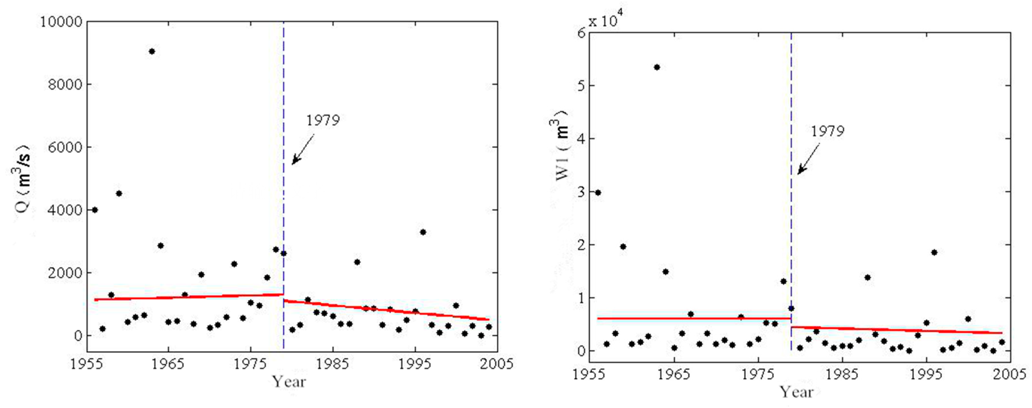
Firstly, we adopted the pettitt test and Mann-Kendall test to detect the change point and trend of the annual maximum flood peak Q and one-day flood volume W₁ time series. Through pettitt test, the possible change points for the Q sequence are 1979 and 1996, and for W₁ 1979 and 1982. Since the test probability P of 1979 is the largest, and it is among the change points of both Q and W₁ sequences, the most possible change point is 1979. This agrees with the results obtained by other researchers using different methods [32].

Before the trend analysis, the autocorrelation analysis of the flood sequences should be carried out. Since the autocorrelation coefficients of both the Q and W₁ sequences are less than 0.1, it is considered that the autocorrelation of these sequences is not significant, so the trend test can be conducted directly. Without considering the change point, the non-parametric Mann-Kendall test was used to analyze the trend of the flood sequences. The statics $U_n$ of flood sequences Q and W₁ are both less than −1.96, which shows that the flood sequences have passed the test at a significance of 5% and present a downward trend.

In order to consider the influence of the change point on the trend test, the Q and W₁ sequences were divided into two subsequences and tested by non-parametric Mann-Kendall test method, respectively. Figure 2 shows the test results of the subsequences: although the subsequence of Q before 1979 shows a slight upward trend, and the subsequences of Q and W₁ after 1979 show a downward trend, none of them passed the test of significance. Meanwhile, no trend has been found for the sequence of W₁ before 1979.

In the case of full flood sequences presenting a significant downward trend, while the subsequences with 1979 as the dividing point showing no significant trend, the latter is more suitable for describing the inconsistency of the flood sequences.

4.2. Nonstationary Model of Univariate Flood Frequency Analysis with Time as Covariate

4.2.1. Model Fitting Evaluation

A univariate nonstationary model with different distribution functions based on GAMLSS with time as covariate has been constructed based on the inflow flood sequences of Wangkuai Reservoir. In order to avoid an over-fitting problem due to excessive freedom degree, this study only considered the linear relationship between the distribution parameters and time t. The parameters include the distribution parameter ${\theta }_1$ (mean value of flood sequence) and ${\theta }_2$ (variance of flood sequence). The optimal fitting distribution, the optimal covariates of the distribution parameters, and the functional relationship between the distribution parameters and the optimal covariates were determined by the AIC criterion.

Table 1. The functional relationships of the explanatory variables and distribution parameters.

Distributions	Q			W1
	AIC	θ1	θ2	AIC	θ1	θ2
Gumbel	895.80	t	-	1074.23	t	-
Weibull	786.60	t	-	928.57	t	-
Gamma	785.99	t	-	930.55	t	-
Log-Normal	783.92	t	-	919.26	t	-

shows that, for flood peak (Q) and flood volume (W₁) sequences, Weibull distribution and Gamma distribution had similar fitting effect, while log-normal distribution performed best with a minimum value of AIC. The functional relationships are written as Equation (20) for Q and Equation (21) for W₁. For all the distribution models, the optimal covariates of the distribution parameters have been proved to satisfy the significant level 0.05 via ${\chi }^2$ test. Besides, for both Q and W₁ time series, the distribution parameter ${\theta }_1$ presents a linear dependent relationship with time t, whereas ${\theta }_2$ is constant. Therefore, it can be concluded that the variation of the inflow flood sequences of Wangkuai Reservoir is mainly reflected by the mean value rather than the variance.

$${\theta }_1=77.769-0.036t,{\theta }_2=1.030\left(for\mathrm{Q}\right)$$

(20)

$${\theta }_1=84.876-0.039t,{\theta }_2=1.193\left(for{\mathrm{W}}_1\right)$$

(21)

Based on the above analysis, log-normal distribution was selected as the optimal distribution of both flood peak and volume. The corresponding residuals of the optimal distributions and the Filliben coefficients are shown in

Table 2. The residuals of the optimal distributions and corresponding Filliben coefficients.

Flood Series	Optimal Distribution	Mean	Variance	Coefficient of Skewness	Coefficient of Kurtosis	Filliben Coefficient
Q	Log-Normal	0	1.021	−0.357	3.408	0.9895
W1	Log-Normal	0	1.021	0.249	2.402	0.9925

. For a sample size of 49, when the Filliben coefficients are both greater than 0.975, they satisfy the significant level 0.05 via T test. Thus, the model residuals of both Q and W₁ sequences are acceptable and in normal distribution.

4.2.2. Model Results Analysis

The summary of the associated results of the univariate nonstationary model is shown in Figure 3. Most of the observed data points are distributed in the grayscale range between 5% to 95% quantiles, indicating that the model results are able to capture the nonstationarity of the flood data. With time t as covariate, flood peak and volume time series show a downward trend over time. Especially when the quantile is larger (such as 95% quantile), the decrease trend is more significant. This proves that variation of flood sequences has occurred under the changing environment, and the traditional “stationarity” hypothesis has become questionable. Thus, use of the traditional hydrological frequency analysis method may result in inaccurate results. The change of the flood sequences are mainly caused by climate change, land use change, and construction of Water conservancy projects [33,34,35]. Besides, the downward trend is significant before 1980, and tends to be gentle after 1980. This may be due to the change of land use. As revealed by Li et al. [34], water area, agricultural land, and grassland area decreased, while the forest area increased significantly in the control basin of Wangkuai Reservoir during 1970–1980, but from 1980 to 2000, the land use types kept almost invariant.

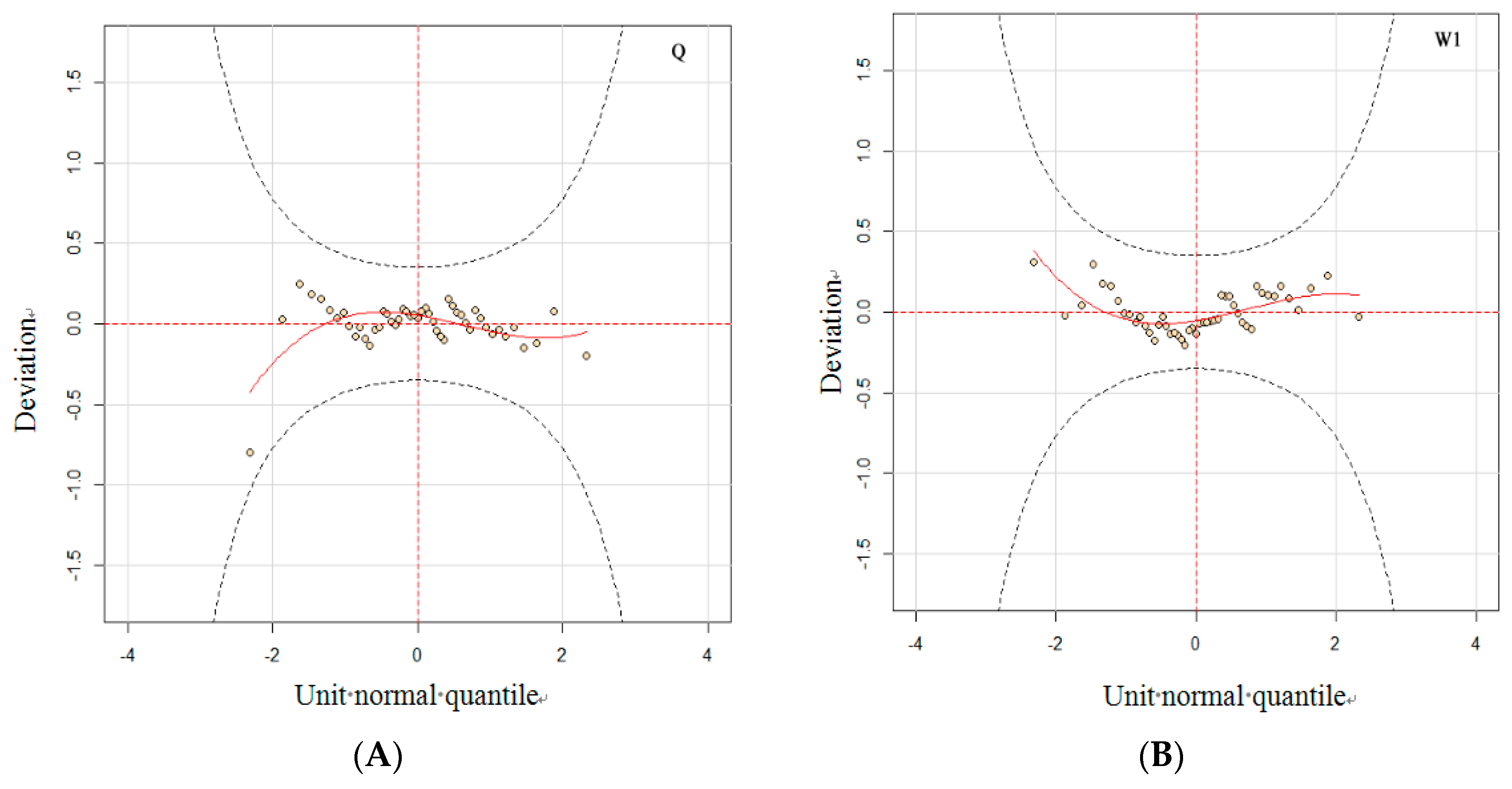
Figure 4 and Figure 5 show the worm plot and normal QQ of the peak discharge Q and one-day volume W₁. As can be seen, no significant departure from normality has been highlighted. Therefore, the results of residuals supported the inference that log-normal distribution provides a good fit to both Q and W₁.

4.3. Nonstationary Model of Bivariate-Joint Flood Frequency Analysis with Time as Covariate

4.3.1. Parameters Calculation, Fitting Test, and Result Optimization of Joint Probability Distribution

With the above two log-normal distributions (Equations (19) and (20)) as marginal distributions, the joint distribution model of flood peak and volume based on copulas have been constructed according to Equations (9)–(11). The parameter of Copula functions $\theta$, K-S test statistic D, and values of OLS and AIC were estimated by Equations (12)–(16). A significance level of $\alpha =0.05$ was used for the K-S test, and the corresponding standard quantile was approximately 0.1943 for n = 49. This means that when D-value is less than 0.1943, it passes the test. The results of the calculation, test, and optimization are presented in

Table 3. The estimation of copula parameters and the associated fitting test and model selection.

Copulas	Copula Parameter (θ)	Indices of Fitting Test and Model Selection
		D (K-S)	OLS	AIC
Gumbel-Hougaard Copula	2.9224	0.1648	0.0404	−312.3751
Clayton Copula	1.6444	0.1940	0.0470	−297.7266
Frank Copula	9.1480	0.2537	0.0469	−297.7374

.

It can be observed in Table 3 that Gumbel-Hougaard copula function and Clayton copula function have passed the K-S test, while the Frank Copula has not passed the test. Among them, the Gumbel-Hougaard copula function has the minimum values of OLS and AIC, indicating that the Gumbel-Hougaard copula function is more suitable to describe the extreme sequence of hydrological variables, such as the joint distribution of flood peak and volume. Therefore, the G-H Copula with parameter $\theta =2.9224$ was considered as the optimal copula for the bivariate-joint distribution of the Q and W₁ time series of Wangkuai Reservoir.

4.3.2. Most Likely Combination of the Flood Peak and Volume

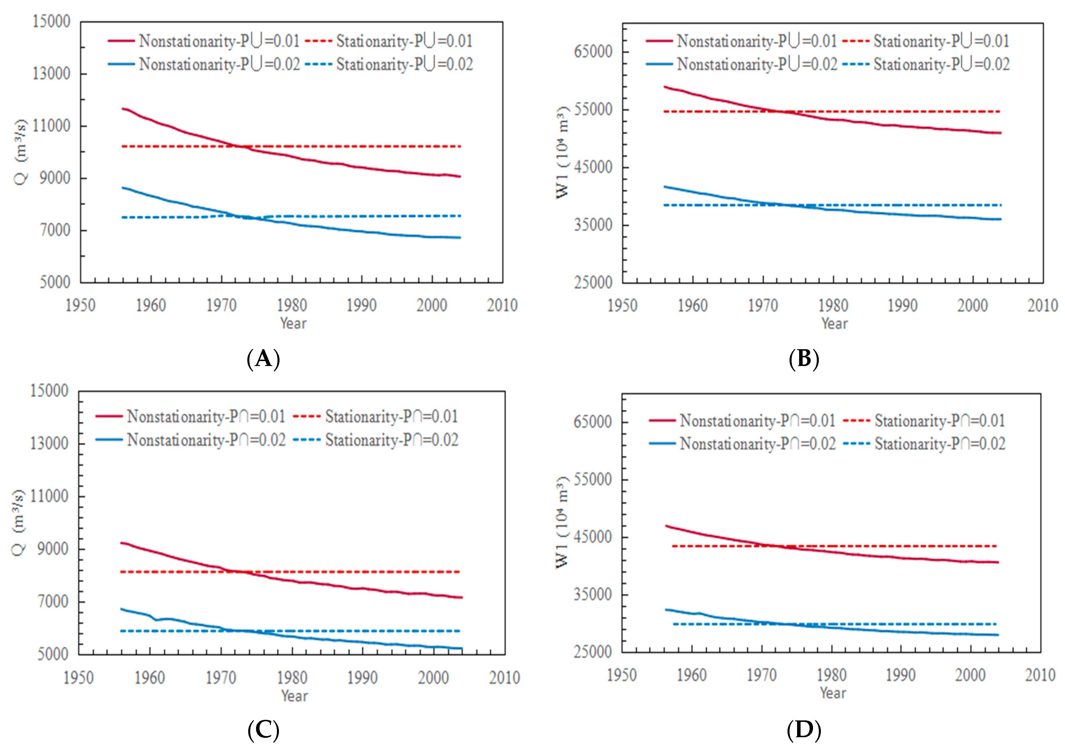
The “most likely” design events derived from Equation (11) have their maximum value of likelihood function on each probability-isoline, and all combinations of Q and W₁ were illustrated in Figure 6. They have the similar undulating behavior as the univariate models shown in Figure 3.

Figure 6 shows that, under changing environmental conditions, with time t as the covariate of the marginal distribution, the combination values of the flood peak and volume under the same OR-joint and AND-joint exceedance probability both display a decreasing trend. Meanwhile, the combination values of the nonstationary model intersect with the traditional stationary results between 1970–1980. That is, before 1970, the most likely combination values considering the variation of distribution parameters over time were larger than fixed parameters (stationary), however, they were smaller after 1980.

5. Discussion and Conclusions

The changing environment makes the assumption of stationarity of flood sequences questionable. In this context, this paper constructed both univariate and bivariate nonstationary models with time as covariate based on GAMLSS theory for flood frequency analysis. The inflow flood peak Q and flood volume W₁ series of Wangkuai Reservoir were used as basic data.

Within the framework of nonstationary flood frequency, this paper adopted four two-parameter distributions (Gumbel, Weibull, Gamma, and Log-Normal) as alternative distributions, which have the characteristics of power distribution and exponential distribution simultaneously. In the univariate nonstationary model with time as covariate, log-normal distribution performed best according to AIC criterion. The flood peak and volume time series presented a decreasing trend over time. Especially when the quantile is high (such as 95% quantile), the downward trend is more significant. Besides, the decreasing trend is significant before 1980, and tends to be gentle after 1980. This proves that variation of flood sequences has occurred under the changing environment.

Based on the optimal univariate models, copula functions were addressed to construct the dependence structure of Q and W₁, with the two optimal log-normal distributions as marginal distributions. The results showed that only the Gumel-Hougaard copula can provide the best joint distribution. The most likely events have similar undulating behavior to the univariate models, and the combination values of the flood peak and volume under the same OR-joint and AND-joint exceedance probability both display a decreasing trend. Meanwhile, the combination values of the nonstationary model intersect with the traditional stationary results between 1970–1980. That is, before 1970, the most likely combinations considering the variation of distribution parameters over time were larger than fixed parameters (stationary), whereas it became the opposite after 1980.

References

- Zheng, F.; Westra, S.; Leonard, M.; Sisson, S.A. Modeling dependence between extreme rainfall and storm surge to estimate coastal flooding risk. Water Resour. Res. 2014, 50, 205–2071. [Google Scholar] [CrossRef]
- Milly, P.C.D.; Betancourt, J.; Falkenmark, M.; Hirsch, R.M. Stationarity is dead: Whither water management. Science 2008, 319, 573–574. [Google Scholar] [CrossRef] [PubMed]
- Ishak, E.H.; Rahman, A.; Westra, S.; Sharma, A.; Kuczera, G. Evaluating the non-stationarity of Australian annual maximum flood. J. Hydrol. 2013, 494, 134–145. [Google Scholar] [CrossRef]
- Salas, J.D.; Obeysekera, J. Revisiting the concepts of return period and risk for nonstationary hydrologic extreme events. J. Hydrol. Eng. 2014, 19, 554–568. [Google Scholar] [CrossRef]
- Waylen, P.; Woo, M.K. Prediction of annual floods generated by mixed processes. Water Resour. Res. 1982, 18, 1283–1286. [Google Scholar] [CrossRef]
- Singh, V.P.; Wang, S.X.; Zhang, L. Frequency analysis of nonidentically distributed hydrologic flood data. J. Hydrol. 2005, 307, 175–195. [Google Scholar] [CrossRef]
- Cunderlik, J.M.; Burn, D.H. Non-stationary pooled flood frequency analysis. J. Hydrol. 2003, 276, 210–223. [Google Scholar] [CrossRef]
- Vasiliades, L.; Galiatsatou, P.; Loukas, A. Nonstationary frequency analysis of annual maximum rainfall using climate covariates. Water Resour. Manag. 2015, 29, 339–358. [Google Scholar] [CrossRef]
- Rigby, R.A.; Stasinopoulos, D.M. Generalized additive models for location, scale and shape. J. R. Stat. Soc. Ser. C (Appl. Stat.) 2005, 54, 507–554. [Google Scholar] [CrossRef]
- Stasinopoulos, D.M.; Rigby, R.A. Generalized additive models for location scale and shape (GAMLSS) in R. J. Stat. Softw. 2007, 23, 1–46. [Google Scholar] [CrossRef]
- Boutselis, P.; Ringrose, T.J. GAMLSS and networks in combat simulation metamodelling: A case study. Expert Syst. Appl. 2013, 40, 6087–6093. [Google Scholar] [CrossRef]
- Luo, J.W.; Chen, L.N.; Liu, H. Distribution characteristics of stock market liquidity. Phys. A Stat. Mech. Appl. 2013, 382, 6004–6014. [Google Scholar] [CrossRef]
- Wahl, S.; Fenske, N.; Zeilinger, S.; Suhre, K.; Gieger, C.; Waldenberger, M.; Grallert, H.; Schmid, M. On the potential of models for location and scale for genome-wide DNA methylation data. BMC Bioinform. 2014, 15, 1471–2105. [Google Scholar] [CrossRef] [PubMed]
- Serinaldi, F.; Kilsby, C.G. A modular class of multisite monthly rainfall generators for water resource management and impact studies. J. Hydrol. 2012, 464–465, 528–540. [Google Scholar] [CrossRef]
- López, J.; Francés, F. Non-stationary flood frequency analysis in continental Spanish rivers, using climate and reservoir indices as external covariates. Hydrol. Earth Syst. Sci. 2013, 17, 3189–3203. [Google Scholar] [CrossRef] [Green Version]
- Hawkes, P.J. Joint probability analysis for estimation of extremes. J. Hydraul. Res. 2008, 46, 246–256. [Google Scholar] [CrossRef]
- Fiorentino, M.; Gioia, A.; Iacobellis, V.; Manfreda, S. Regional analysis of runoff thresholds behaviour in Southern Italy based on theoretically derived distributions. Adv. Geosci. 2011, 26, 139–144. [Google Scholar] [CrossRef] [Green Version]
- Zheng, F.; Westra, S.; Sisson, S.A. Quantifying the dependence between extreme rainfall and storm surge in the coastal zone. J. Hydrol. 2013, 505, 172–187. [Google Scholar] [CrossRef]
- Mirabbasi, R.; Fakheri-Fard, A.; Dinpashoh, Y. Bivariate drought frequency analysis using the copula method. Theor. Appl. Climatol. 2012, 108, 191–206. [Google Scholar] [CrossRef]
- Zhang, L.; Singh, V.P. Bivariate rainfall frequency distributions using Archimedean copulas. J. Hydrol. 2007, 332, 93–109. [Google Scholar] [CrossRef]
- Fu, G.; Butler, D. Copula-based frequency analysis of overflow and flooding in urban drainage systems. J. Hydrol. 2014, 510, 49–58. [Google Scholar] [CrossRef] [Green Version]
- Li, J.; Liu, X.; Chen, F. Evaluation of Nonstationarity in Annual Maximum Flood Series and the Associations with Large-scale Climate Patterns and Human Activities. Water Resour. Manag. 2015, 29, 1653–1668. [Google Scholar] [CrossRef]
- Li, J.; Tan, S. Nonstationary Flood Frequency Analysis for Annual Flood Peak Series, Adopting Climate Indices and Check Dam Index as Covariates. Water Resour. Manag. 2015, 29, 5533–5550. [Google Scholar] [CrossRef]
- Zeng, H.; Feng, P.; Li, X. Reservoir flood routing considering the non-stationarity of flood series in north China. Water Resour. Manag. 2014, 28, 4273–4287. [Google Scholar] [CrossRef]
- Cole, T.J.; Green, P.J. Smoothing reference centile curves: The lms method and penalized likelihood. Stat. Med. 2010, 11, 1305–1319. [Google Scholar] [CrossRef]
- Filliben, J.J. The Probability Plot Correlation Coefficient Test for Normality. Technometrics 1975, 17, 111–117. [Google Scholar] [CrossRef]
- Sklar, A. Fonctions de Répartition À N Dimensions Et Leurs Marges; Institut de Statistique Université de Paris: Paris, France, 1959; pp. 229–231. [Google Scholar]
- Nelsen, R.B. An Introduction to Copulas; Springer: New York, NY, USA, 2006. [Google Scholar]
- Akaike, H. A new look at the statistical model identification. IEEE Trans. Autom. Control 1974, 19, 716–723. [Google Scholar] [CrossRef]
- Olsen, J.R.; Stedinger, J.R.; Matalas, N.C.; Stakhiv, E.Z. Climate variability and flood frequency estimation for the Upper Mississippi and Lower Missouri Rivers. J. Am. Water Resour. Assoc. 1999, 35, 1509–1524. [Google Scholar] [CrossRef]
- Gräler, B.; van den Berg, M.J.; Vandenberghe, S.; Petroselli, A.; Grimaldi, S.; De Baets, B.; Verhoest, N.E.C. Multivariate return periods in hydrology: A critical and practical review focusing on synthetic design hydrograph estimation. Hydrol. Earth Syst. Sci. 2013, 17, 1281–1296. [Google Scholar] [CrossRef] [Green Version]
- Li, X.; Zeng, H.; Feng, P. Flood frequency analysis considering variation in flood time series. J. Hydroelectr. Eng. 2014, 33, 11–19. [Google Scholar]
- Wang, Y.; Li, J.; Feng, P.; Chen, F. Effects of large-scale climate patterns and human activities on hydrological drought: a case study in the luanhe river basin, China. Nat. Hazards 2015, 76, 1687–1710. [Google Scholar] [CrossRef]
- Li, J.; Li, G.; Zhou, S.; Chen, F. Quantifying the Effects of Land Surface Change on Annual Runoff Considering Precipitation Variability by SWAT. Water Resour. Manag. 2016, 30, 1071–1084. [Google Scholar] [CrossRef]
- Gu, X.; Zhang, Q.; Chen, X.; Jiang, T. Nonstationary flood frequency analysis considering the combined effects of climate change and human activities in the East River Basin. Trop. Geogr. 2014, 34, 746–757. [Google Scholar]
Figure 1.
The study area: Wangkuai Reservoir in the Daqinghe river basin with the Wangkuai Reservoir watershed in the upper-left corner.
Figure 2.
Trend test results of the flood subsequences with consideration of change point.
Figure 3.
Summary of results of the univariate nonstationary model with Generalized Additive Models in Location, Scale, and Shape (GAMLSS) implementation. Red points represent the observed time series of peak discharge Q (A) and flood volume W1 (B). The solid black line represents 0.5 quantile; the dark grey region is the area between 0.25 and 0.75 quantiles; the light grey region is the area between 0.05 and 0.95.
Figure 4.
Worm plot of the residuals of non-stationary time-varying model with GAMLSS implementation (Q in A, W1 in B). For a satisfactory fit of worm plot, all the observations should fall inside the two elliptic curves.
Figure 5.
QQ plot of the residuals of non-stationary time-varying model with GAMLSS implementation (Q in A, W1 in B).
Figure 6.
Results of the most likely design events (combinations of flood peak and volume). Case illustration for (A,B) and (C,D).