Article

Using SWAT-LUD Model to Estimate the Influence of Water Exchange and Shallow Aquifer Denitrification on Water and Nitrate Flux

by
Xiaoling Sun
1,2,3,*,
Léonard Bernard-Jannin
3,4,
Youen Grusson
3,5,6,
Sabine Sauvage
3,
Jeffrey Arnold
7,
Raghavan Srinivasan
8 and
José Miguel Sánchez Pérez
3,*
1
School of Environmental Science and Engineering, Southern University of Science and Technology of China, Shenzhen 518055, China
2
State Key Laboratory of Water Resources and Hydropower Engineering Science, Wuhan University, Wuhan 430072, China
3
Laboratoire d’Ecologie Fonctionnelle et Environnement (ECOLAB), UMR 5245 CNRS-UPS-INPT Ecole Nationale Supérieure Agronomique de Toulouse (ENSAT), Avenue de l’Agrobiopole BP 32607 AuzevilleTolosane, France
4
Institut des Sciences de la Terre d’Orléans (ISTO), UMR 7327 Université d’Orléans-CNRS-BRGM, 1A rue de la Férollerie 45100 Orléans, France
5
Chaire de Recherche EDS en Previsions et Actions Hydrologiques, Department of Civil and Water Engineering, Université Laval, Québec City, QC G1V 0A6, Canada
6
Swedish University of Agricultural Sciences Department of Soil and Environment, Division of Soil Physics, P.O. Box 7014, SE-750 07 Uppsala, Sweden
7
Grassland, Soil & Water Research Laboratory USDA-ARS, Temple, TX 76502, USA
8
Spatial Science Laboratory in the Department of Ecosystem Science and Management, Texas A&M University, College Station, TX 77845, USA
*
Authors to whom correspondence should be addressed.
Water 2018, 10(4), 528; https://doi.org/10.3390/w10040528
Submission received: 26 February 2018 / Revised: 2 April 2018 / Accepted: 6 April 2018 / Published: 23 April 2018
(This article belongs to the Section Water Quality and Contamination)

Abstract

:
Numerous studies have pointed out the importance of groundwater and surface water interaction (SW–GW) in a river system. However; those functions have rarely been considered in large scale hydrological models. The SWAT-LUD model has been developed based on the Soil and Water Assessment Tool (SWAT) model; and it integrates a new type of subbasin; which is called subbasin-LU (SL); to represent the floodplain area. New modules representing SW–GW exchanges and shallow aquifer denitrification are developed in the SWAT-LUD model. In this study; the SWAT-LUD model was applied to the middle floodplain area of the Garonne catchment in France. The results showed that the SWAT-LUD model could represent the SW–GW exchange and shallow aquifer denitrification appropriately. An annual 44.1 × 10⁷ m3 of water flowed into the river from the study area; but the annual exchanged water volume was 6.4 × 10⁷ m3; which represented just 1% of the river discharge. A total of 384 tons of N-NO3 (0.023 t·ha−1) was consumed by denitrification in the floodplain shallow aquifer annually. The nitrate concentration (N-NO3) decrease in the channel was 0.12 mg·L−1; but in the shallow aquifer it reached 11.40 mg·L−1; 8.05 mg·L−1; and 5.41 mg·L−1 in LU1; LU2; and LU3; respectively. Our study reveals that; in the Garonne floodplain; denitrification plays a significant role in the attenuation of nitrate associated with groundwater; but the impacts of denitrification on nitrate associated with river water is much less significant.

1. Introduction

Up to 90% of floodplains are cultivated in Europe and North America, and floodplains have been found to be vulnerable regions of nitrate pollution [1,2]. Extensive surface water and groundwater exchange occurs in the floodplain area, and hydrologic connectivity links floodplain and river into an integrated eco-hydro-system. As surface water (SW) contains oxygen and organic matter and groundwater (GW) contains abundant nutrient elements, the interaction between them has been found to have significant influence on biotic communities and ecosystem processes of both river and shallow aquifer ecosystems [3,4].
Riparian zones are buffer zones located between terrestrial and aquatic ecosystems [4]. Studies have proposed that denitrification in riparian areas is an important process that decreases the nitrate load of groundwater [5,6,7]. The impact of riparian hydrology on denitrification has been highlighted [8], and it has been suggested that denitrification may be strongly influenced in the riparian zone by the hydrogeological setting and the hydraulic properties of the underlying geological deposits [9]. Most of these studies have focused on the denitrification process occurring in the soil layer of riparian zone, and the importance of the shallow aquifer on nitrate eliminating has been ignored. However, it has been proven that denitrification in the shallow aquifer also plays an important role in nitrate depletion [10,11]. Different from in the soil layer, organic carbon is identified as the major factor limiting denitrification rates in a shallow aquifer system [5]. Riparian zones with higher groundwater levels increase the interaction between groundwater and surface soil with rich organic matter and lead to more intensive denitrification [12].
SW–GW interaction is a complex process that is driven by geomorphology, hydrogeology, and climate conditions [13]. Most of the models dealing with the SW–GW exchange process are distributed models, such as MODFLOW, MOHID, or 2SWEM. This type of model requires spatial inputs with high-resolution, numerous parameters, and significant computation time, and the requirements inhibit their application on large scales. The river/groundwater interface is rarely included in large scale, conceptual hydrological models. To overcome this issue, conceptual and distributed models have been incorporated, such as SWAT-MODFLOW, WATLAC, and WASIM-ETH-I-MODFLOW, but the limitations of distributed models still exist in these incorporated models. Modeling has been proven to be an efficient tool to estimate the denitrification rates in a large-scale catchment. The denitrificatin process has been included in many models, but most of the models have only considered the denitrification process in the soil profile; few of them take into account the influence of denitrification in the shallow aquifer on nitrate elimination [14]. The Soil and Water Assessment Tool (SWAT) model is a catchment scale model, which has been successfully applied all over the world. However, the SW–GW exchange and denitrification occurring in the shallow aquifer are not simulated by the SWAT model. To represent the SW–GW exchange in the floodplain, a new type of subbasin, which is called subbasin-LU (SL), was developed in the SWAT model. The modified model is called the SWAT-LUD model [15]. The influence of the SW–GW exchange and flooding on nitrate cycling was incorporated into the model, and the shallow aquifer denitrification function was also included.
The SWAT-LUD model has been applied to one SL in previous studies and has shown its ability to quantify the SW–GW-exchanged water volume and the shallow aquifer denitrification rate correctly [15,16]. However, the previous studies of the SWAT-LUD model focused on the riparian area only, and the impacts of the SW–GW exchange on river water flow and the influence of denitrification occurring in the shallow aquifer on river water nitrate were not evaluated. In this study, the SWAT-LUD model is applied to the middle floodplain area of the Garonne River in France. The objective of this study are: (i) to quantify the impacts of water exchanges on river water discharge, and (ii) to estimate the influence of denitrification resulted in nitrate elimination in both river water and groundwater associated nitrate pollution.

2. Materials and Methods

2.1. SWAT-LUD Model

2.1.1. Hydrological Processes in the SWAT-LUD Model

The SWAT model includes three spatial entities to represent the spatial heterogeneity: basin, subbasins, and hydrologic response units (HRUs). The basin is divided into subbasins, and subbasins are then divided into HRUs. HRUs are combinations of land cover, soil type, and slope. In the SWAT model, processes are simulated in each HRU and then aggregated at the subbasin scale by the weighted averages of the HRUs, while the natural downward flow path inside the subbasin is not represented [17,18]. The SWAT catena delineation method was developed by dividing the subbasin into upland divide, hillslope, and valley bottom based on slope. With this method, the water flow in the subcatchment is considered as a single track: water flows from the upland divide to the hillslope before entering the valley bottom. The groundwater level in each unit and the SW–GW exchange are not considered with this method [
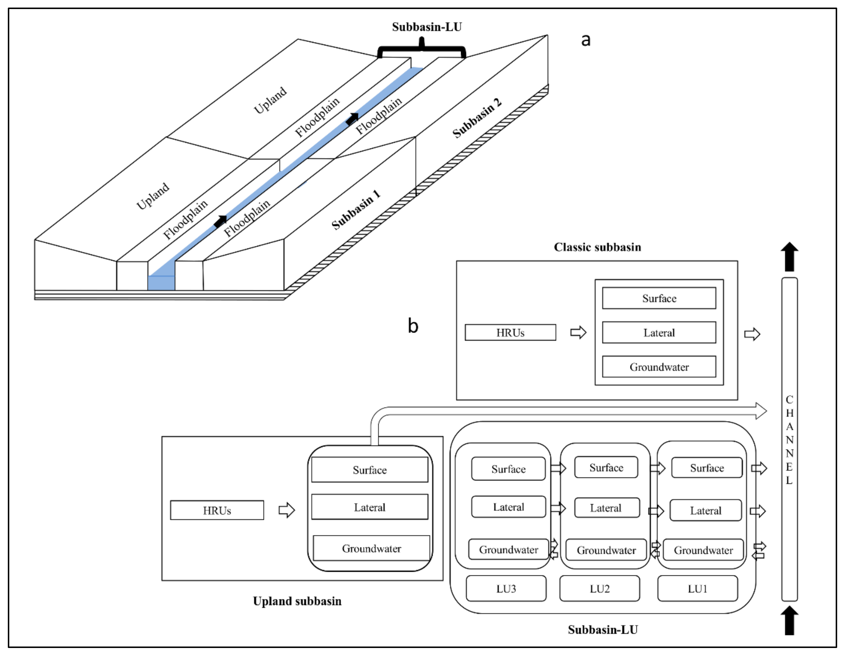
19]. To represent the SW–GW exchange occurring in the floodplain, the SWAT model is modified by splitting the original SWAT subbasin that holds alluvial soil along the channel into two types of subbasins: the subbasin-LU (SL) and the upland subbasin. The modified model is called the SWAT-LUD model. Thus, three types of subbasins exist in the SWAT-LUD model, which are the classic subbasin, the upland subbasin, and the SL. Classic subbasins are the original SWAT subbasins without alluvial soil along the existing channel. Each original SWAT subbasin that contains alluvial soil along the channel is separated into two subbasins, the upland subbasin and the SL. The upland subbasin corresponds to the upper area of the subbasin (without alluvial soil), while the SL corresponds to the alluvial soil area.
In the SWAT-LUD model, an additional unit called a landscape unit (LU), which is a structure between a subbasin and a HRU, is applied in the subbasin-LU. Each subbasin-LU contains three LUs, and HRUs are distributed across the LUs. LUs are delineated with the catena delineation method, and the three LUs in each SL are the divide (LU3), the hillslope (LU2), and the valley bottom (LU1). LU3 is located farthest from the channel, LU2 is located in the middle, and LU1 is located next to the channel. Because alluvial soils are commonly associated with floodplains, the locations of the subbasin-LUs were considered to be the same as the locations of alluvial soil. The widths of LUs are defined based on the return period area within the floodplain: LU1 takes 10% of the floodplain area, LU2 takes 20% of the area, and LU3 takes 70% of the area.
The hydrological processes in the SWAT-LUD model are shown in Figure 1. The processes in the classic subbasin and the upland subbasin remain the same as in the original SWAT model. In the subbasin-LU, surface water and lateral water flow from LU3 routing through LU2 into LU1 before entering the channel. The water exchange between the surface water and groundwater is performed with Darcy’s equation. The recharged flooded water on flooding days and the transfer of dissolved elements along with the water are simulated as well. A detailed description of the hydrological processes can be found in [15] by Sun et al.

2.1.2. Denitrification in the SWAT-LUD Model

In the subbasin-LU, the denitrification process in the soil profile is remains the same as in the original SWAT model except when groundwater arrives at the soil profile. Under this condition, the soil profile is considered to be the shallow aquifer. The denitrification process in the shallow aquifer of the floodplain remains the same as in the previous SWAT-LUD model [16]. The denitrification process considers the influence of organic carbon from both the water and soil/aquifer sediment on the denitrification rate. Dissolved organic carbon (DOC) is the organic carbon originating from the water and particulate organic carbon (POC) is the organic carbon originating from the soil/aquifer sediment.
The nitrate attenuation rate is calculated as follows:
R N O 3 , i = 0.8 ( ρ · ( 1 φ ) / φ · k P O C [ POC i ] · 10 6 / M c + k D O C [ D O C i ] ) · [ N O 3 , i ] / ( k N O 3 + [ N O 3 , i ] )
where R N O 3 , i is the denitrification rate (µ mol·L−1·day−1) on day i, ρ is the dry sediment density (kg·dm−3), φ is the sediment porosity, k P O C is the mineralization rate constant of POC (day−1), POC is the POC content in the soil and aquifer sediment on day i (‰), M c is the carbon molar mass (g·mol−1), DOC is the concentration of DOC in the aquifer water on day i (µ mol·L−1),   k D O C is the constant mineralization rate of DOC (day−1), k N O 3 is half-saturation for nitrate limitation (µ mol·L−1), and N O 3 is the nitrate concentration in the aquifer water on day i (µ mol·L−1).
The consumption rates of DOC and POC are simplified first-order decay:
R D O C = k D O C [ DOC i ]
where RDOC is the DOC consumption rate on day i (µ mol·L−1·day−1).
R P O C = k P O C [ POC i ]
where RPOC is the POC consumption rate on day i (‰·day−1).
On flooding days, a portion of the nitrate in the soil profile infiltrates into the shallow aquifer along with the infiltrate-flooded river water. The infiltrated nitrate content is calculated as follows:
M N O 3 , i =   M N O 3 , i 1 + I N O 3 , i
I N O 3 , i = F N O 3 × M N O 3 ,   s o i l , i
where M N O 3 , i is the mass content of nitrate in the LU (g N-NO3) on day i, M N O 3 , i 1 is the mass content of nitrate in the LU (g N-NO3) on day i-1, I N O 3 is the infiltrated mass of nitrate from the soil profile into the aquifer during flood events on day i (g N-NO3),   F N O 3 is the coefficient representing the fraction of the leached nitrates (%), and M N O 3 ,   s o i l , i is the mass content of nitrate in the soil profile of LU (g N-NO3) on day i.

2.2. Distribution of HRUs in LUs

As subbasin-LUs contain just alluvial soils, in each subbasin-LU, HRUs are simplified into three subcategories based on land-use type: forest alluvial HRU (F-HRU), pasture alluvial HRU (P-HRU), and agricultural alluvial HRU (A-HRU). The alluvial HRUs with all types of forest land cover are integrated into one F-HRU. The characteristic of the F-HRU is considered to be the same as the largest forest alluvial HRU before the integration. The alluvial HRUs with pasture land cover or land types similar to the characteristics of pasture (such as orchard or vineyard) are integrated into one P-HRU, and the alluvial HRUs with agriculture land use are integrated into one A-HRU. The characteristics of these two HRUs are chosen by the same method as that for the F-HRU: taking the characteristics of the largest HRU before the integration.
The natural distribution of land use in alluvial areas is characterized by the succession of riparian forest, pasture, and agriculture from the river to the hillside. Based on this succession of land use, the distribution of HRUs into LUs is as follows: First, the F-HRU is assigned into LU1. If the area of the F-HRU is larger than LU1, then the F-HRU is split into two HRUs, one corresponding to the area of LU1 and the other corresponding to the remaining area. If the area of the F-HRU is smaller than LU1, then all the F-HRU is assigned into LU1, and the empty area in LU1 is taken up by the P-HRU. In this case, if the P-HRU area is larger than the empty area in LU1, then the P-HRU is split into two HRUs, one corresponding to the empty area in LU1 and the other corresponding to the remaining area. If P-HRU is smaller than the empty area in LU1, then all the P-HRU is assigned into LU1 and the remaining area in LU1 is filled by the A-HRU. Under this condition, the A-HRU is divided into two HRUs. The same method is applied to distribute the HRUs into LU2 and LU3. HRUs of the same type are assumed to have the same characteristics.

2.3. Study Site

The Garonne River has a drainage area of about 51,500 km2 and a length of 525 km at the last gauging station not influenced by tidal (Tonneins). The average annual rainfall is around 900 mm [20]. The study area is located in the middle of the Garonne River, between Toulouse and the confluence with the Tarn River (Figure 2). The width of the floodplain is 2–4 km. The coarse alluvium of 4–7 m (sand and gravel) eroded from the Pyrenees Mountains during the past glacial periods overlie an impermeable molassic bedrock [21]. A series of terraces exists in the floodplain, and the higher terrace delimits the floodplain. Field studies show that the impermeable substratum of the higher terrace is placed above the topographical surface of the floodplain, and the floodplain is disconnected from the larger scale upland aquifer [21]. The middle terrace, which is around 2 km wide, is cultivated and rarely flooded (every 30–50 years). The lower terrace, with a width of a few hundred meters devoted to poplar plantations, is flooded every year or every two years. The riparian zone is flooded almost every year and has a width of 10–100 m [22].
The floodplain is intensively cultivated, with high production of corn, sunflower, and sorghum sustained by fertilization and irrigation. The shallow aquifer has a nitrate concentration (N-NO3) of 10–25 mg·L−1 [11,23,24]. The channel in the study area is a meandering, single-thread channel and has a length of 85 km and a mean sinuosity coefficient of 1.3. The Portet gauging station is located about 10 km upstream of Toulouse (Figure 2). The average daily flow at this station is around 200 m3·s−1, but it ranges from 20 m3·s−1 to 4300 m3·s−1 (Banque Hydro, http://www.hydro.eaufrance.fr/). The study area is around 4600 km2, and according to the soil map of European soil database (ESDB), the alluvial soil along the main channel takes up around 4% of the total area. Four piezometers with continuous records of groundwater levels documented by the Bureau de Recherches Géologiques et Minières (BRGM) are located within the study site (P91, P170, P286, and P3247, Figure 2).
The Monbéqui site is located in a meander of the alluvial plain. From May 2004 to July 2005, groundwater samples from five piezometers were taken monthly except during August and September 2004. From April 2013 to March 2014, groundwater samples from 28 piezometers and two river points were taken monthly for analysis of physicochemical parameters. A detailed description of piezometer distribution can be found in [15] by Sun et al. Water samples were taken only when the electrical conductivity of the extracted groundwater was constant to ensure that the water sample corresponded to the aquifer and not to stagnant water [25]. Water samples were then filtered through 0.45 µm cellulose acetate membrane filters. Nitrate (NO3) and chloride (Cl) were determined by ion chromatography (Dionex ICS-5000+ and DX-120). To determine the DOC concentrations, water samples were filtered through rinsed 0.45-µm cellulose acetate membrane filters, stored in carbon-free glass tubes, acidified with HCl, and combusted using a platinum catalyzer (Shimadzu, Model TOC 5000) at 650 °C. In order to determine the POC content, shallow aquifer sediment samples were taken seasonally. The sediment was sampled after water sampling by increasing the pumping velocity for 5–10 min with the water flowing into a 50-L tank, where sediments settled before being collected together with 100 mL water in sealed sterile bags. To obtain ash-free dry mass (AFDM) content, which is expressed as a percentage of the dry sediment weight, the sediment samples were dried (105 °C, 24 h) and combusted (550 °C, 4 h).

2.4. Definition and Parameters of Subbasin-LUs and LUs

In this study, the surface areas of LU1, LU2, and LU3 were considered to be 10%, 20%, and 70% of the alluvial soil area, respectively, which correspond to the flood return periods of the Garonne River (1 year, 2–5 years, and 10 or more years). The SL and LU parameters are presented in Table 1. SL1 is the subbasin-LU near the Portet gauging station, which is located in the upstream part of the study area, SL2 is the subbasin-LU in the middle of the floodplain, and SL3 is the subbasin-LU farthest from the Portet gauging station, which is located downstream of the study area. Porosity values were obtained from field and modeling studies of Seltz [26] and Weng et al. [27].
The crop rotations applied in the agricultural areas were determined based on the studies of the Save River, which is subbasin 9 in the study area [28,29] (Table 2).
The observed daily discharges at the Portet gauging station (Figure 2c) were applied as input data to represent the river water discharges from the upstream area. The nitrate concentration in the river water was considered as a constant 1.13 mg·L−1 (N-NO3), which was given based on the nitrate concentrations measured at the Blagnac station (located downstream of Toulouse, Figure 2c) taking into account the influence of the urban area of Toulouse (www.eaufrance.fr). The nitrate concentrations in the LUs were simulated by the model.
Studies have found that the further away from the river, the more stable the DOC concentrations [16]. In our study, the DOC concentrations in LU2 and LU3 were assumed to be constant. The input DOC concentrations in the LUs and in the river water were determined based on the measurements at Monbéqui in 2013. The DOC concentrations in LU1 were calculated based on the DOC concentrations in the river water and LU2. As the DOC concentration in the river water significantly increases on flooding days [30,31,32], we used two DOC concentration values to distinguish the difference, one for no flooding days and another higher value for flood periods.
The POC pool was separated into two parts: the top layer pool and the second layer pool. The topsoil layer was considered to be 0.5 m thick, and the second layer was considered to be the soil layer underneath the topsoil (from 0.5 m to the bottom of the soil profile). The POC content was regarded as 50% of the AFDM content in the soil in accordance with recent studies [33,34,35]. The POC content values in the topsoil layers and second layers were from Jego’s study [24] and the AFDM values were from measurements in the alluvial sediment in 2013, respectively. The organic carbon content in all three SLs were the same (Table 3).

2.5. Calibration and Evaluation

The calibration was performed automatically for the original SWAT parameters and manually for the newly developed SWAT-LUD parameters. The automatic calibration was performed with SWAT-CUP, which is an external software tool permitting SWAT users to realize automatic calibration with more comfort and efficiency [36]. SWAT-CUP includes several possible algorithms, of which SUFI-2 is known to achieve better calibration performance in a limited number of iterations [37]. The observed discharges from the Larra, Verdun, and Lamagistère gauging stations (see station locations in Figure 2c) were used for calibration. Sensitivity analysis and calibration were performed by SWAT-CUP with the SUFI-2 algorithm [38]. After sensitive parameters were identified, a 1500-run calibration was performed as recommended by Yang et al. [37].
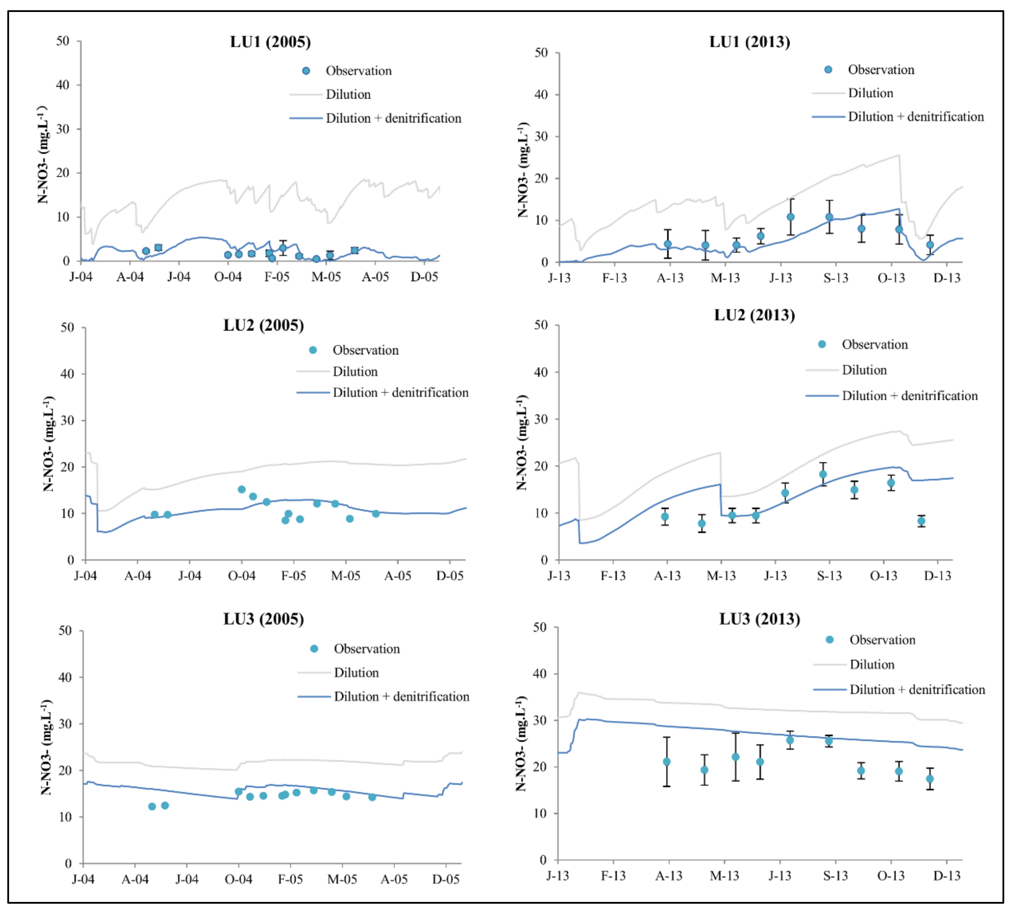
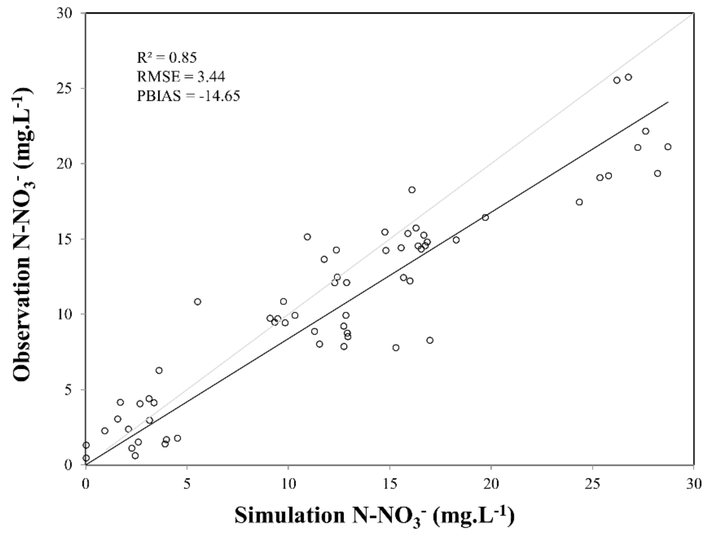
Because the SW–GW exchange and shallow aquifer denitrification processes were not included in the SWAT model, the parameters of these functions could not be calibrated by SWAT-CUP. Therefore, manual calibration was carried out to adjust the newly developed parameters. The observed groundwater levels in the four BRGM piezometers, P91, P170, P286, and P3247 (
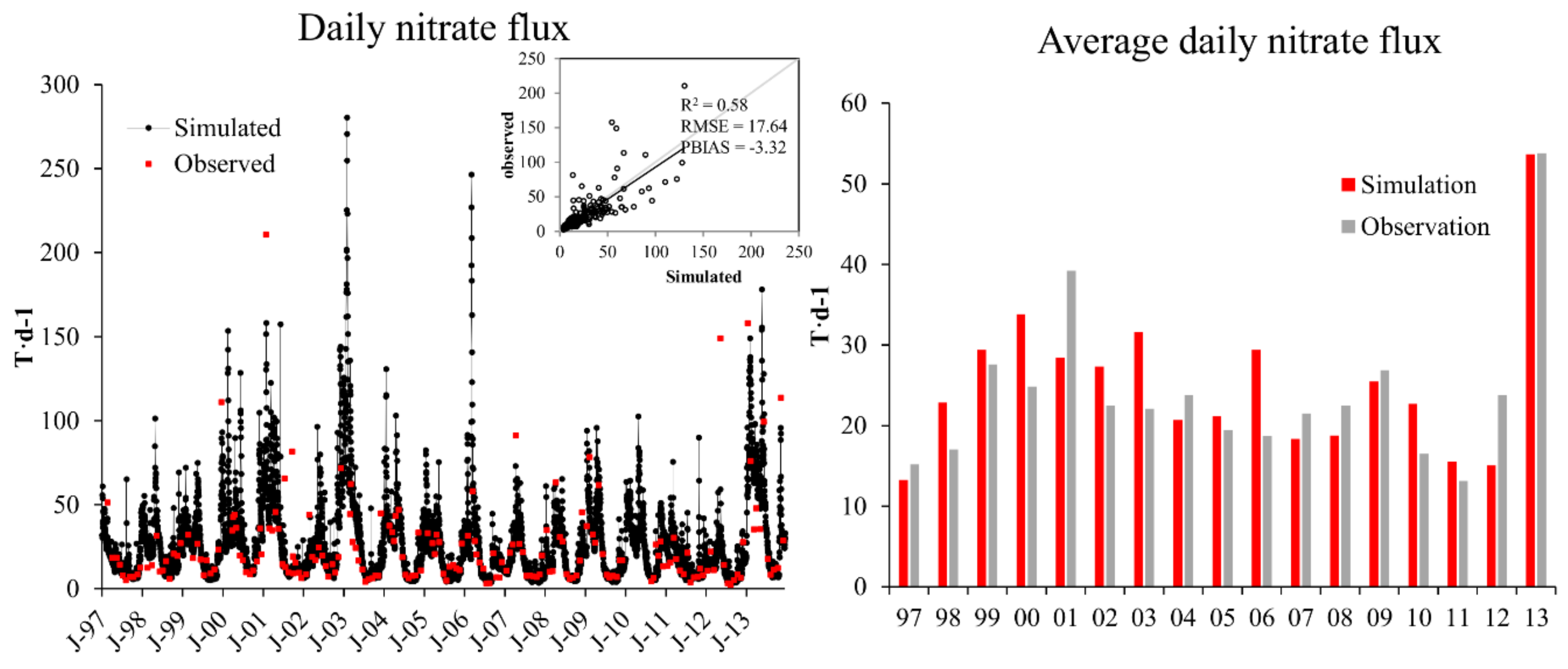
Figure 2), were used to calibrate the river water exchange. The nitrate concentrations in the shallow aquifer, which were measured in 2004–2005 and 2013 at Monbéqui, were used to calibrate the denitrification process. In 2013, nitrate concentrations were measured in six piezometers in LU1, 14 piezometers in LU2, and three piezometers in LU3, and in 2004–2005, nitrate concentrations were measured in two piezometers in LU1, one piezometer in LU2, and one piezometer in LU3. The measured nitrate concentrations were also used to calibrate the model. The nitrate fluxes observed at the St-Aignan station were used to validate the nitrate flux output simulated at the outlet of the simulated area. The evaluation of the quality of the simulation included the percent bias (PBIAS), the root means square error (RMSE), and the coefficient of determination (R2).

3. Results

3.1. Calibrated Parameters

The characteristics of the automatically calibrated parameters are shown in Table 4. It must be noted that the parameters and their calibrated values vary among subbasins.
Parameters related to the new processes in the SWAT-LUD model were calibrated manually and are presented in Table 5.
In total, 15 parameters were automatically calibrated with the observed discharge from the Larra, Verdun, Lamagistère, and Portet gauging stations using the SWAT-CUP (detailed information can be found in the study by Grusson et al. [39]). CH_Ns were calibrated manually with the groundwater levels documented by the Bureau de Recherches Géologiques et Minières (BRGM), and the other 11 parameters were manually calibrated with the measured nitrate concentrations at the Monbéqui site. Because the underground nitrate concentrations were recorded only at Monbéqui, these 11 manually calibrated values were applied to all three subbasin-LUs.

3.2. Surface Water–Groundwater Exchange

3.2.1. Groundwater Level

The simulated groundwater levels were compared with the observed values, and the results are shown in Figure 3.
The results showed that the model could represent the groundwater variation in all the three LUs without considering the water connection with the upland area. The groundwater levels were slightly overestimated, with the PBIAS criterion values varying from −0.85% to −4.61%. The best match occurred in LU2 of SL2, while the worst match occurred in LU3 of SL3. Except for the results of LU3 in SL1, the variations of the simulated groundwater levels were larger than those of the observations, and the groundwater levels on the most intense flooding days that occurred in 2000 were overestimated.

3.2.2. Water Balance in the Study Area

The annual water balance in the study area is shown in Figure 4.
An annual 511.9 × 10⁷ m3 of water flowed into the river from the upstream river, and the simulated area contributed another 44.1 × 10⁷ m3. Among all three subbasin types, the classic subbasins provided the maximum volume of water, which is 26.2 × 10⁷ m3, representing up to 59.4% of the total water volume originated from the study area. The upland subbasin supplied another 11.3 × 10⁷ m3 of water, and 6.6 × 10⁷ m3 of water flowed into the river from the subbasin-LU. In the opposite direction, a total amount of 2.0 × 10⁷ m3 of river water entered the shallow aquifer per year.
River water entered the shallow aquifer through surface infiltration (flood) and lateral infiltration. In the Garonne River, surface infiltrated river water volume contributed 40% of the total infiltrated river water volume. In the subbasin-LU, groundwater originated from both rainfall infiltration and river water infiltration. In our study, the annual groundwater flow was 4.4 × 10⁷ m3, accounting for 66.6% of the total water yield. Since an annual 2.0 × 10⁷ m3 of river water infiltrated into the groundwater, the annual recharged rainfall was 2.4 × 10⁷ m3, which is similar to the infiltrated river water volume. The total exchanged water volume was 6.4 × 10⁷ m3, which was the sum of the groundwater flow and the river water infiltration, representing just 1% of the water volume that flow through the river.

3.3. Nitrate Concentration in the Shallow Aquifer

The comparison of the simulated nitrate concentrations in LUs with the values observed at the Monbéqui site over two periods (2004–2005 and 2013) are shown in Figure 5.
The evaluation of the performance of the simulated nitrate concentrations is shown in Figure 6.
Figure 5 and Figure 6 reveal that a nitrate concentration gradient is shown in the LUs: the concentration increases with the distance from the river. The simulated nitrate concentrations that considered denitrification have good agreement with the observed values. With the consideration of denitrification, the nitrate concentration was slight overestimated, especially in LU3, the simulations were higher than the observed values. In our study site, denitrification consumed nitrate in the shallow aquifer significantly, with the nitrate concentration (N-NO3) reducing by 11.40 mg·L−1, 8.05 mg·L−1, and 5.41 mg·L−1 in LU1, LU2, and LU3, respectively, over the simulated period. The residual nitrate concentrations in the three LUs are 3.86 mg·L−1, 11.38 mg·L−1, and 17.95 mg·L−1, respectively.

3.4. Nitrate Balance

The simulated daily nitrate flux at the outlet of the studied area and the observed values from St-Aignan gauging station are shown in Figure 7. The average daily nitrate flux over the entire simulated period is also presented in Figure 7. Overall, the model could reproduce the observation accurately, leading to an RMSE criterion of 17.64 t·day−1. The nitrate flux was overestimated in 2000, 2003, and 2006 and underestimated in 2001 and 2012. The nitrate flux over the whole simulated period was slightly overestimated (PBIAS = −3.32%), but the nitrate flux in low flow period was better simulated.
The annual nitrate balance in the study area is shown in Figure 8.
A total of 6038 tons of N-NO3 came from the upstream river per year, and the study area contributed another 3479 tons to the river. Similarly to the water flux, nitrate mostly came from the classic subbasin and the upland subbasin; these two subbasin types supplied 97.4% of the total nitrate flux to the study area. In contrast with the water flux, the subbasin-LUs contributed just 2.6% of the total nitrate flux. In the subbasin-LUs, 96 tons of nitrate flowed into the river from the shallow aquifer, while only 24 tons of nitrate in the river water entered the shallow aquifer.
A total of 384 tons (0.023 t·ha−1) N-NO3 were consumed per year through denitrification in the shallow aquifer of floodplain, corresponding to 79% of the nitrate originating from the subbasin-LUs and 4% of the nitrate flowing out of the study site in the river (9622 tons). The denitrification rate in LU1 was much higher than in the other LUs. Nitrate originated from LU3 and LU2, flowed into LU1, and was consumed through the denitrification process. The nitrate concentration (N-NO3) in the river was reduced by 0.12 mg·L−1. The annual denitrification rate occurring in the three LUs in the shallow aquifer of the subbasin-LUs are shown in Table 6, suggesting that the denitrification rate in LU1 was much higher than that in the other two LUs.

4. Discussion

4.1. SWAT-LUD Model

Physically based models and lumped conceptual models are key model types in hydrological study. Different from a physically based model, the SW–GW exchange process occurring along the river is not considered in most of the lumped conceptual models [40,41]. The SWAT-LUD model represents an interesting intermediate between the physically based and the lumped conceptual models. In the SWAT-LUD model, each LU represents a reservoir, and Darcy’s equation is applied to quantify the water exchanged between the LUs, while the remaining watershed is simulated with the original semi-distributed SWAT model. This combination allows the SWAT-LUD model to be applied on a large watershed with considering the processes occurring on the local near-bank floodplain. In the SWAT-LUD model, the hydrological process of the upland subbasin remains the same in as the original SWAT model, water from HRUs enters the channel directly instead of follow the flow path. In most rivers, water from the upland will flow into the adjacent floodplain; however, in certain rivers such as the Garonne River, the shallow aquifer of the floodplain is isolated from the upland shallow aquifer [21].
Hydrological exchange occurring along the river and the related biogeochemical reactions have been studied for more than 50 years, and the research of the SW–GW flow on a small spatial scale has become increasingly feasible. The challenges that the research community are now facing are to apply the acquired knowledge to larger scales [42]. In the SWAT-LUD model, the application of Darcy’s equation and a simple denitrification equation has allowed the estimation of water exchange and nitrate attenuation in the floodplain area on the catchment scale with a limited number of parameters. This model could help to understand the water and nitrate cycling processes in the critical biogeochemical zone at on a large scale.

4.2. Surface Water and Groundwater Exchange

The impacts of SW–GW exchanges on river water discharge in the study site are estimated. An annual 5.5 × 10⁹ m3 of water flow through the river, but the annual exchanged water volume was 6.4 × 10⁷ m3, which represented only 1% of the river discharge. This demonstrated that the influence of water exchange on river water discharge is not significant in our study. This conclusion, however, depends on the location and the geomorphological condition of the river. A study dealing with the Mississippi River network revealed that all the water in the reach that arrived at the outlet of the river network had circulated through the lateral exchange, and the SW–GW exchange ratio was higher in the headwater than in the downstream area [43]. Based on the research throughout the whole United States, headwaters comprise around 53% of the total stream length [44]. Our study site is located in the middle floodplain area of the Garonne River, a substantially higher exchange ratio is expected in the Garonne watershed if the headwaters were considered.
Unlike the limited influence on river water discharge, the impacts of the SW–GW exchange on water flow in the subbasin-LUs were much more significant. An annual 2.0 × 10⁷ m3 of water flowed into the shallow aquifer from the river, corresponding to 50% of the groundwater flow of the subbasin-LUs. The infiltrated flooded water, which is ignored by most of the large-scale models, contributed 40% of the total water volume that flowed from the river into the groundwater. The study of Krause and Bronstert [45] indicated that the interaction between groundwater and surface water has a major importance for the water balance and is periodically superimposed on the vertical runoff generation. The study of Bernard-Jannin et al. [46] at the Monbéqui site also indicated that the water volume infiltrated through the floodplain surface is seven times higher than the water volume infiltrated through the river bank over a simulated five-month period during which one flooding event occurred. Besides infiltration, the floodwater retention also has a great influence on biogeochemical activities; it created anaerobic conditions and supplemented the contact area with the rich, organic carbon-contented top soil [47].

4.3. Nitrate Flux and the Influence of Denitrification

Floodplains could be both sources and sinks of nitrate. A large amount of nitrate leaches from cultivated plains into groundwater [48,49], while in the natural floodplain, nitrate could be eliminated through denitrification and plant uptake [50]. The reported nitrate elimination rates of the floodplains range from 7% to 68% [51,52]. In the Garonne River, the floodplain is widely cultivated: most parts of the floodplain, including LU3 and parts of LU2, are cultivated, and only the LU1 strips that are located close to the river are mainly covered with natural riparian forest. An annual total of 6038 tons of N-NO3 comes from the upstream river water with a drainage area of 13,700 km2. The amount of nitrate originating from the study area reached 3479 tons per year, which is a large value relative to the accumulated area (4600 km2), and the study area was thus considered to be an important nitrate source. The floodplain area represented by the subbasin-LU was proven to be a source of nitrate, providing an annual total of 102 tons of nitrate. However, different from other catchments, water and nitrate from the upland subbasin flowed into the river instead of into the floodplain in the Garonne River, and the nitrate that flowed to the river was nitrate generated from the floodplain area.
The nitrate degradation rates in the floodplain have been studied in various rivers with different nitrate sources. Hester et al. [53] estimated the influence of the restored inset floodplain on nitrate reduction in a second-order restoration river (width of 3.5 m, discharge of 0.059 m3·s−1), and less than 1% of the inflowing mass was removed within a 90 m reach. In a study about the Atchafalaya River during the 2011 Mississippi River flooding, 7% of the river-associated N-NO3 was found to be retained in the floodplain along the 192 km reach [51]. In our study site, only 24 tons of nitrogen–nitrate entered the floodplain from the river water every year, while the annual nitrate flux in the river reached 9622 tons. The floodplains are well-known critical nitrate removal areas; however, few studies separately quantified the nitrate elimination originating from groundwater and from river water. In our study, the nitrate concentration (N-NO3) reduction in the channel was 0.12 mg·L−1, but in the shallow aquifer it reached 11.40 mg·L−1, 8.05 mg·L−1, and 5.41 mg·L−1 in LU1, LU2, and LU3, respectively. This reveals that denitrification plays a significant role in the attenuation of nitrate associated with groundwater, but the impacts of denitrification on nitrate associated with river water is much less significant.

5. Conclusions

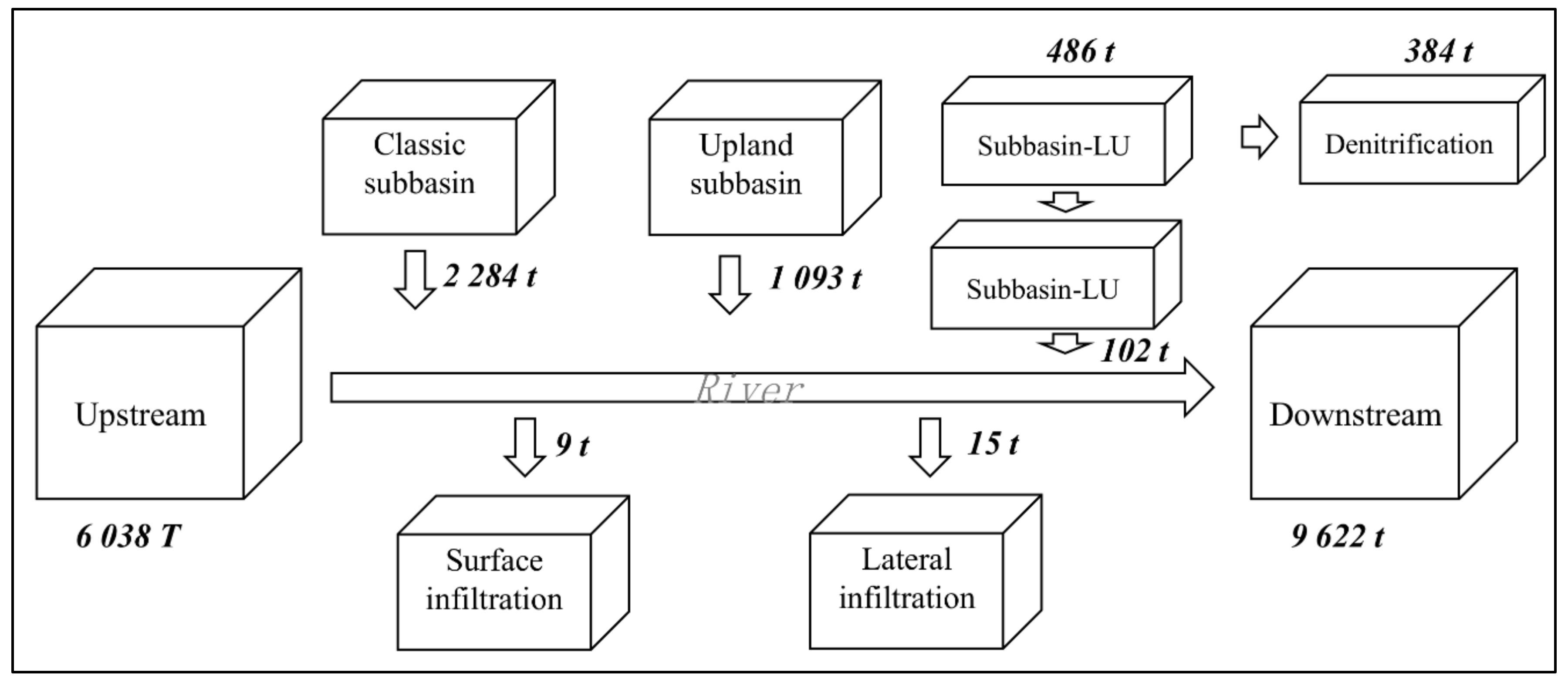
In this paper, the SWAT-LUD model was applied to the middle floodplain of the Garonne River in France. The SW–GW exchange at the river–floodplain interface and the denitrification in the shallow aquifer were simulated and quantified. The results showed that the SWAT-LUD model could represent the SW–GW exchange and the shallow aquifer denitrification appropriately. Among all three subbasin types, the classic subbasins provided the maximum volume of water, which was 26.2 × 10⁷ m3, representing up to 59.4% of the total volume of water originating from the study area. A total of 6.6 × 10⁷ m3 of water flowed into the river from the subbasin-LU. In the opposite direction, a total amount of 2.0 × 10⁷ m3 of river water entered the shallow aquifer per year, and the surface infiltration during the flood period engaged 40% of the infiltrated river water. The annual exchanged water volume represented only 1% of the river discharge. An annual 384 tons of N-NO3 was consumed by denitrification in the floodplain shallow aquifer. The nitrate concentration (N-NO3) decrease in the channel was 0.12 mg·L−1, but in the shallow aquifer it reached 11.40 mg·L−1, 8.05 mg·L−1, and 5.41 mg·L−1 in LU1, LU2, and LU3, respectively. Our study revealed that denitrification plays a significant role in the attenuation of nitrate associated with groundwater, and the impacts of denitrification on nitrate associated with river water is much less significant.

Acknowledgments

This work was supported by the National Key R&D program of China [grant number 2016YFC0402806]; Shenzhen Science and Technology Innovation Commission program [grant number JCYJ20160429191638556]; Shenzhen Peacock Plan [grant number KQTD2016022619584022]; the National Key R&D Program of China [grant number 2016YFC0401404]; the European Regional Development Fund [SOE3/P2/F55800]; and the French National Research Agency [ANR-11-CEPL-008]. We are grateful to Samuel Teissier for his help in the field and with laboratory work.

Author Contributions

José Miguel Sánchez Pérez and Sabine Sauvage conceived of the structure of this study; Léonard Bernard-Jannin and Youen Grusson contributed the field data and model calibration; Jeffery Arnold and Raghavan Srinivasan contributed the building of the new module; Xiaoling Sun wrote the paper.

Conflicts of Interest

The authors declare no conflict of interest. The founding sponsors had no role in the design of the study; in the collection, analyses, or interpretation of data; in the writing of the manuscript; or in the decision to publish the results.

References

  1. Cey, E.E.; Rudolph, D.L.; Aravena, R.; Parkin, G. Role of the riparian zone in controlling the distribution and fate of agricultural nitrogen near a small stream in southern Ontario. J. Contam. Hydrol. 1999, 37, 45–67. [Google Scholar] [CrossRef]
  2. Huan, H.; Wang, J.; Zhai, Y.; Xi, B.; Li, J.; Li, M. Quantitative evaluation of specific vulnerability to nitrate for groundwater resource protection based on process-based simulation model. Sci. Total Environ. 2016, 550, 768–784. [Google Scholar] [CrossRef] [PubMed]
  3. Hug, P.D.; Castella, E.; Slaveykova, V.I. Lateral and longitudinal patterns of water physico-chemistry and trace metal distribution and partitioning in a large river floodplain. Sci. Total Environ. 2017, 587–588, 248–257. [Google Scholar]
  4. Gregory, S.V.; Swanson, F.J.; McKee, W.A.; Cummins, K.W. An Ecosystem Perspective of Riparian Zones. BioScience 1991, 41, 540–551. [Google Scholar] [CrossRef]
  5. Hill, A.R. Nitrate Removal in Stream Riparian Zones. J. Environ. Qual. 1996, 25, 743. [Google Scholar] [CrossRef]
  6. Martin, T.L.; Kaushik, N.K.; Trevors, J.T.; Whiteley, H.R. Review: Denitrification in temperate climate riparian zones. Water Air Soil Pollut. 1999, 111, 171–186. [Google Scholar] [CrossRef]
  7. Maítre, V.; Cosandey, A.-C.; Desagher, E.; Parriaux, A. Effectiveness of groundwater nitrate removal in a river Riparian area: The importance of hydrogeological conditions. J. Hydrol. 2003, 278, 76–93. [Google Scholar] [CrossRef]
  8. Rassam, D.W.; Pagendam, D.E.; Hunter, H.M. Conceptualisation and application of models for groundwater—Surface water interactions and nitrate attenuation potential in Riparian zones. Environ. Model. Softw. 2008, 23, 859–875. [Google Scholar] [CrossRef]
  9. Vidon, P.; Hill, A.R. Denitrification and patterns of electron donors and acceptors in eight riparian zones with contrasting hydrogeology. Biogeochemistry 2005, 71, 259–283. [Google Scholar] [CrossRef]
  10. Iribar, A. Composition des Communautés Bactériennes Dénitrifiantes au Sein d’un Aquifère Alluvial et Facteurs Contrôlant Leur Structuration: Relation Entre Structure des Communautés et Dénitrification. Ph.D. Thesis, Université Toulouse III—Paul Sabatier, Toulouse, France, 2007. [Google Scholar]
  11. Sánchez-Pérez, J.M.; Vervier, P.; Garabétian, F.; Sauvage, S.; Loubet, M.; Rols, J.L.; Bariac, T.; Weng, P. Nitrogen dynamics in the shallow groundwater of a riparian wetland zone of the Garonne, SW France: Nitrate inputs, bacterial densities, organic matter supply and denitrification measurements. Hydrol. Earth Syst. Sci. Discuss. 2003, 7, 97–107. [Google Scholar] [CrossRef] [Green Version]
  12. Gold, A.J.; Groffman, P.M.; Addy, K.; Kellogg, D.Q.; Stolt, M.; Rosenblatt, A.E. Landscape Attributes as Controls on Groithd Water Nitrate Removal Capacity of Riparian Zones. J. Am. Water Resour. Assoc. 2001, 37, 1457–1464. [Google Scholar] [CrossRef]
  13. Sophocleous, M. Interactions between groundwater and surface water: The state of the science. Hydrogeol. J. 2002, 10, 52–67. [Google Scholar] [CrossRef]
  14. Heinen, M. Simplified denitrification models: Overview and properties. Geoderma 2006, 133, 444–463. [Google Scholar] [CrossRef]
  15. Sun, X.; Bernard-Jannin, L.; Garneau, C.; Volk, M.; Arnold, J.G.; Srinivasan, R.; Sauvage, S.; Sánchez-Pérez, J.M. Improved simulation of river water and groundwater exchange in an Alluvial plain using the SWAT model. Hydrol. Process. 2016, 30, 187–202. [Google Scholar] [CrossRef] [Green Version]
  16. Sun, X.; Bernard-Jannin, L.; Sauvage, S.; Garneau, C.; Arnold, J.G.; Srinivasan, R.; Sánchez-Pérez, J.M. Assessment of the denitrification process in alluvial wetlands at floodplain scale using the SWAT model. Ecol. Eng. 2017, 103, 344–358. [Google Scholar] [CrossRef]
  17. Arnold, J.G.; Srinivasan, R.; Muttiah, R.S.; Williams, J.R. Large Area Hydrologic Modeling and Assessment Part I: Model Development. J. Am. Water Resour. Assoc. 1998, 34, 73–89. [Google Scholar] [CrossRef]
  18. Lam, Q.D.; Schmalz, B.; Fohrer, N. Modelling point and diffuse source pollution of nitrate in a rural lowland catchment using the SWAT model. Agric. Water Manag. 2010, 97, 317–325. [Google Scholar] [CrossRef]
  19. Bosch, D.D.; Arnold, J.G.; Volk, M.; Allen, P.M.; Douglasmankin, K.R.; Srinivasan, R.; Arnold, J.G. Simulation of a low-gradient coastal plain watershed using the SWAT landscape model. Trans. ASABE 2010, 53, 1445–1456. [Google Scholar] [CrossRef]
  20. Caballero, Y.; Voirin-Morel, S.; Habets, F.; Noilhan, J.; LeMoigne, P.; Lehenaff, A.; Boone, A. Hydrological sensitivity of the Adour-Garonne river basin to climate change. Water Resour. Res. 2007, 43, W07448. [Google Scholar] [CrossRef]
  21. Lancaster, R.R. Fluvial Evolution of the Garonne River, France: Integrating Field Data with Numerical Simulations. Master’s Thesis, Louisiana State University, Baton Rouge, LA, USA, 2005. [Google Scholar]
  22. Peyrard, D.; Sauvage, S.; Vervier, P.; Sanchez-Perez, J.M.; Quintard, M. A coupled vertically integrated model to describe lateral exchanges between surface and subsurface in large alluvial floodplains with a fully penetrating river. Hydrol. Process. 2008, 22, 4257–4273. [Google Scholar] [CrossRef]
  23. Pinay, G.; Ruffinoni, C.; Wondzell, S.; Gazelle, F. Change in Groundwater Nitrate Concentration in a Large River Floodplain: Denitrification, Uptake, or Mixing? J. N. Am. Benthol. Soc. 1998, 17, 179–189. [Google Scholar] [CrossRef]
  24. Jego, G. Influence Des Activités Agricoles sur la Pollution Nitrique des Eaux Souterraines. Analyse par Modélisation des Impacts des Systèmes de Grande Culture sur les Fuites de Nitrate dans les Plaines Alluviales. Ph.D. Thesis, Université Toulouse III—Paul Sabatier, Toulouse, France, 2008. [Google Scholar]
  25. Sánchez-Pérez, J.M.; Trémolières, M.; Carbiener, R. Une station d’épuration naturelle des phosphates et nitrates apportés par les eaux de débordement du Rhin: La forêt alluviale à frêne et orme. Comptes Rendus de L'Académie des Sciences 1991, 312, 395–402. [Google Scholar]
  26. Seltz, R. Analyse et Modélisation D’une Zone Humide Riveraine de la Garonne; L’Ecole de Physique du Globe de Strasbourg: Strasbourg, France, 2001. [Google Scholar]
  27. Weng, P.; Sánchez-Pérez, J.M.; Sauvage, S.; Vervier, P.; Giraud, F. Assessment of the quantitative and qualitative buffer function of an alluvial wetland: Hydrological modelling of a large floodplain (Garonne River, France). Hydrol. Process. 2003, 17, 2375–2392. [Google Scholar] [CrossRef]
  28. Boithias, L. Modélisation des Transferts de Pesticides à L’échelle des Bassins Versants en Période de Crue. Ph.D. Thesis, Université Toulouse III—Paul Sabatier, Toulouse, France, 2012. [Google Scholar]
  29. Boithias, L.; Srinivasan, R.; Sauvage, S.; Macary, F.; Sánchez-Pérez, J.M. Daily Nitrate Losses: Implication on Long-Term River Quality in an Intensive Agricultural Catchment of Southwestern France. J. Environ. Qual. 2014, 43, 46. [Google Scholar] [CrossRef] [PubMed]
  30. Arango, C.P.; Tank, J.L.; Schaller, J.L.; Royer, T.V.; Bernot, M.J.; David, M.B. Benthic organic carbon influences denitrification in streams with high nitrate concentration. Freshw. Biol. 2007, 52, 1210–1222. [Google Scholar] [CrossRef]
  31. Dalzell, B.J.; Filley, T.R.; Harbor, J.M. Flood pulse influences on terrestrial organic matter export from an agricultural watershed. J. Geophys. Res. Biogeosci. 2005, 110. [Google Scholar] [CrossRef]
  32. Duan, S.; Bianchi, T.S.; Sampere, T.P. Temporal variability in the composition and abundance of terrestrially-derived dissolved organic matter in the lower Mississippi and Pearl Rivers. Mar. Chem. 2007, 103, 172–184. [Google Scholar] [CrossRef]
  33. Griffiths, N.A.; Tank, J.L.; Royer, T.V.; Warrner, T.J.; Frauendorf, T.C.; Rosi-Marshall, E.J.; Whiles, M.R. Temporal variation in organic carbon spiraling in Midwestern agricultural streams. Biogeochemistry 2012, 108, 149–169. [Google Scholar] [CrossRef]
  34. Hauer, F.R.; Lamberti, G.A. Methods in Stream Ecology; Academic Press: Cambridge, MA, USA, 2011; ISBN 9780080547435. [Google Scholar]
  35. Wagner, R.; Marxsen, J.; Zwick, P.; Cox, E.J. Central European Stream Ecosystems: The Long Term Study of the Breitenbach; John Wiley & Sons: Hoboken, NJ, USA, 2011; ISBN 9783527634668. [Google Scholar]
  36. Arnold, J.G.; Moriasi, D.N.; Gassman, P.W.; Abbaspour, K.C.; White, M.J.; Srinivasan, R.; Santhi, C.; Harmel, R.D.; Griensven, A.V.; Liew, M.W.V. SWAT: Model use, calibration, and validation. Trans. ASABE 2012, 55, 1345–1352. [Google Scholar] [CrossRef]
  37. Yang, J.; Reichert, P.; Abbaspour, K.C.; Xia, J.; Yang, H. Comparing uncertainty analysis techniques for a SWAT application to the Chaohe Basin in China. J. Hydrol. 2008, 358, 1–23. [Google Scholar] [CrossRef]
  38. Abbaspour, K.C. SWAT-CUP 2012: SWAT Calibration and Uncertainty Programs—A User Manual. Sci. Technol. 2014. [Google Scholar] [CrossRef]
  39. Grusson, Y.; Anctil, F.; Sauvage, S.; Pérez, J.M.S. Assessing the Climatic and Temporal Transposability of the SWAT Model across a Large Contrasted Watershed. J. Hydrol. Eng. 2017, 22, 04017004. [Google Scholar] [CrossRef]
  40. Derx, J.; Blaschke, A.P.; Blöschl, G. Three-dimensional flow patterns at the river-aquifer interface—A case study at the Danube. Adv. Water Resour. 2010, 33, 1375–1387. [Google Scholar] [CrossRef]
  41. Nützmann, G.; Levers, C.; Lewandowski, J. Coupled groundwater flow and heat transport simulation for estimating transient aquifer–stream exchange at the lowland River Spree (Germany). Hydrol. Process. 2014, 28, 4078–4090. [Google Scholar] [CrossRef]
  42. Harvey, J.; Gooseff, M. River corridor science: Hydrologic exchange and ecological consequences from bedforms to basins. Water Resour. Res. 2015, 51, 6893–6922. [Google Scholar] [CrossRef]
  43. Kiel, B.A.; Bayani Cardenas, M. Lateral hyporheic exchange throughout the Mississippi River network. Nat. Geosci. 2014, 7, 413–417. [Google Scholar] [CrossRef]
  44. Nadeau, T.-L.; Rains, M.C. Hydrological Connectivity Between Headwater Streams and Downstream Waters: How Science Can Inform Policy. J. Am. Water Resour. Assoc. 2007, 43, 118–133. [Google Scholar] [CrossRef]
  45. Krause, S.; Bronstert, A. The impact of groundwater–surface water interactions on the water balance of a mesoscale lowland river catchment in northeastern Germany. Hydrol. Process. 2007, 21, 169–184. [Google Scholar] [CrossRef]
  46. Bernard-Jannin, L.; Brito, D.; Sun, X.; Jauch, E.; Neves, R.; Sauvage, S.; Sánchez-Pérez, J.-M. Spatially distributed modelling of surface water-groundwater exchanges during overbank flood events—A case study at the Garonne River. Adv. Water Resour. 2016, 94, 146–159. [Google Scholar] [CrossRef] [Green Version]
  47. Bernard-Jannin, L.; Sun, X.; Teissier, S.; Sauvage, S.; Sánchez-Pérez, J.-M. Spatio-temporal analysis of factors controlling nitrate dynamics and potential denitrification hot spots and hot moments in groundwater of an alluvial floodplain. Ecol. Eng. 2017, 103, 372–384. [Google Scholar] [CrossRef] [Green Version]
  48. Chen, J.; Tang, C.; Sakura, Y.; Yu, J.; Fukushima, Y. Nitrate pollution from agriculture in different hydrogeological zones of the regional groundwater flow system in the North China Plain. Hydrogeol. J. 2005, 13, 481–492. [Google Scholar] [CrossRef]
  49. Shamrukh, M.; Corapcioglu, M.Y.; Hassona, F.A.A. Modeling the Effect of Chemical Fertilizers on Ground Water Quality in the Nile Valley Aquifer, Egypt. Ground Water 2001, 39, 59–67. [Google Scholar] [CrossRef]
  50. Opperman, J.J.; Galloway, G.E.; Fargione, J.; Mount, J.F.; Richter, B.D.; Secchi, S. Sustainable floodplains through large-scale reconnection to rivers. Science 2009, 326, 1487–1488. [Google Scholar] [CrossRef] [PubMed]
  51. Bryantmason, A.; Junxu, Y.; Altabet, M.A. Limited capacity of river corridor wetlands to remove nitrate: A case study on the Atchafalaya River Basin during the 2011 Mississippi River Flooding. Water Resour. Res. 2013, 49, 283–290. [Google Scholar] [CrossRef]
  52. Woltemade, C.J. Ability of Restored Wetlands to Reduce Nitrogen and Phosphorus Concentrations in Agricultural Drainage Water. J. Soil Water Conserv. 2000, 55, 303–309. [Google Scholar]
  53. Hester, E.T.; Hammond, B.; Scott, D.T. Effects of inset floodplains and hyporheic exchange induced by in-stream structures on nitrate removal in a headwater stream. Ecol. Eng. 2016, 97, 452–464. [Google Scholar] [CrossRef]
Figure 1. The hydrological processes of the SWAT-LUD model. (a) The location of the subbasin-LU; (b) the hydrological processes in the classic subbasin, the upland subbasin, and the subbasin-LU (SL). HSU = hydrologic response unit; LU = landscape unit; LU3 = the divide; LU2 = the hillslope; and LU1 = the valley bottom.
Water 10 00528 g001
Figure 2. Location of the study site. (a) The location of the Garonne River; (b) the location of the simulated area; (c) the location of the alluvial soil, Monbéqui site, and piezometers.
Water 10 00528 g002
Figure 3. Simulated and observed groundwater levels in the three subbasin-LUs. The grey lines are the simulated series considering the water connection with the upland area. The black lines are the simulated results without the water connection (the model efficiency criteria values are the performances of black lines). RMSE = root means square error and PBIAS = percent bias.
Water 10 00528 g003
Figure 4. Annual water balance in the study area (unit is 107 m3).
Water 10 00528 g004
Figure 5. Simulated and observed nitrate concentrations in the aquifer of the LUs during the periods of 2004–2005 and 2013, where ‘Dilution’ is the simulated results with the infiltrated river water and ‘Dilution + denitrification’ is the simulated results with the infiltrated river water and denitrification.
Water 10 00528 g005
Figure 6. Observed and simulated (dilution plus denitrification) groundwater nitrate concentration in the two periods (2004–2005 and 2013).
Water 10 00528 g006
Figure 7. Simulated and observed nitrate content at the outlet of the study area. R2 = the coefficient of determination.
Water 10 00528 g007
Figure 8. Annual nitrate (N-NO3) balance in the study area.
Water 10 00528 g008
Table 1. Parameters for the three subbasin-LUs (SL1, SL2, and SL3), the LUs, and the HRUs included in the study site (PAST = pasture; FRSD = forest; and AGRR = agriculture).
Subbasin-LUArea (km2)ChannelLUs
Long (km)Width (m)Altitude (masl)Slope (m/m)PorosityArea (km2)HRUs
Land UseFraction of LU (%)
SL157.2722.11200132.3–106.5LU10.0020.15.73PAST0.1
FRSD0.9
LU20.0050.111.45PAST1.0
LU30.0050.140.09PAST0.36
AGRR0.64
SL287.9540.53200106.5–76.3LU10.0020.18.79FRSD1.0
LU20.0050.117.59PAST0.5
FRSD0.35
AGRR0.15
LU30.0050.161.56AGRR1.0
SL322.2613.0420076.3–65.3LU10.0020.12.23PAST0.7
FRSD0.3
LU20.0050.14.45PAST1.0
LU30.0050.115.58PAST0.1
AGRR0.9
Table 2. Crop rotations applied in the agricultural areas.
YearMonthDayOperationCropManagement and Fertilizer TypeQuantityUnit
1725Tillage Generic Conservation Tillage
1101Tillage Generic Conservation Tillage
2131Tillage Harrow 10 Bar Tine 36 Ft
241PlantCorn
241Fertilization 18-46-00300kg·ha−1
267Fertilization 46-00-00870kg·ha−1
271Irrigation 30mm
2710Irrigation 30mm
2720Irrigation 30mm
281Irrigation 30mm
2820Irrigation 30mm
291Irrigation 30mm
2910Irrigation 30mm
21015Harvest and kill
2111PlantWheat
3125Fertilization 15-15-00400kg·ha−1
3310Fertilization 33-00-00400kg·ha−1
3710Harvest and kill
398Tillage Generic Fall Plowing Operation
441Tillage Harrow 10 Bar Tine 36 Ft
4415PlantSunflower
4415Fertilization 15-15-00600kg·ha−1
4825Harvest and kill
4111PlantWheat
5125Fertilization 15-15-00400kg·ha−1
5310Fertilization 33-00-00400kg·ha−1
5710Harvest and kill
Note: The composition of nutrients of the fertilizer applied are as follow: type 18-46-00, 18% mineral nitrogen, 20.2% mineral phosphors; type 33-00-00, 33% mineral nitrogen; type 15-15-00, 15% mineral nitrogen, 6.6% mineral phosphors; and type 46-00-00, 46% mineral nitrogen.
Table 3. Values of the DOC in the shallow aquifer and river water and the POC in the soil and shallow aquifer sediment for the three subbasin-LUs (sample sites are piezometers and river sites in Monbéqui).
LocationSample SiteDOC (mg·L−1) (Measured)DOC (mg·L−1) (Model Input)AFDM (%) (Measured)POC (>50 cm) (%) (Model Input)POC (Top 50 cm) (%) (Model Input)
LU1 simulated0.55 ± 0.030.2751.5
LU2P110.92 ± 0.150.850.65 ± 0.080.2751.0
P220.83 ± 0.090.46 ± 0.07
LU3P260.66 ± 0.110.650.56 ± 0.070.3251.0
P300.65 ± 0.130.74 ± 0.04
RiverR11.72 ± 0.151.7
R21.69 ± 0.20
River (flooding)R12.56 (n = 1)3
R23.12 (n = 1)
Table 4. Automatically calibrated parameters. Types of parameters: r, relative (the existing parameter value is multiplied by (1 + a given value)); a, absolute (the given value is added to the existing parameter value); v, replace (the existing parameter value is replaced by the given value). -- for the default value means default value is not unique; -- for the value of subbasins means retain the default value.
ParametersDescription File TypeDefault ValueVerdunLarraLamagistère
Subbasin Numbers
5, 4, 6, 891, 2, 7
CN2SCS runoff curve number.mgtr--−0.014−0.040−0.048
ALPHA_BFBaseflow recession constant (1/days).gwv0.0480.440.890.35
GW_DELAYGroundwater delay time (days).gwa31−27.3359.49−23.19
GWQMNThreshold depth of water in the shallow aquifer required for return flow to occur (mm H2O).gwa1000−43.67−77.67181.67
ESCOSoil evaporation compensation factor.hruv0.950.720.720.93
GW_REVAPGroundwater “revap” coefficient.gwv0.020.0620.0280.072
RCHRG_DPDeep aquifer percolation fraction.gwa0.050.0330.0130.0073
CANMXMaximum canopy storage (mm H2O).hruv022.6528.2513.65
CH_K1Effetive hydraulic conductivity in tributary channel alluvium (mm/h).subr03.637.2536.77
SHALLSTInitial depth of water in the shallow aquifer (mm H2O).gwv1000595--958.33
DEEPSTInitial depth of water in the deep aquifer (mm H2O).gwv20003241.67--1865.00
GW_SPYLDSpecific yield of the shallow aquifer (m3/m3).gwr0.0030.17----
GWHTInitial groundwater height (m).gwr10.317.91--
CH_W1Average width of tributary channels (m).subr----−0.020.045
CH_N1Manning’s N value for the tributary channels.subr0.014--−0.011--
Table 5. Manually calibrated parameters.
ParametersDescriptionUnitCalibrated Values
SL1SL2SL3
CH_NManning n--0.070.060.06
KLU1Hydraulic conductivity of LU1m/day100100100
KLU2Hydraulic conductivity of LU2m/day505050
KLU3Hydraulic conductivity of LU2m/day505050
KNO3Half-saturation concentration of nitrateµ mol·L−1303030
kPOC1Kpoc of LU1day−10.5 × 10−50.5 × 10−50.5 × 10⁻⁵
kPOC2Kpoc of LU2day−10.6 × 10−50.6 × 10−50.6 × 10⁻⁵
kPOC3Kpoc of LU3day−10.8 × 10−50.8 × 10−50.8 × 10⁻⁵
kDOC1Kdoc of LU1day−10.0050.0050.005
kDOC2Kdoc of LU2day−10.0020.0020.002
kDOC3Kdoc of LU3day−10.0020.0020.002
FNO3Percentage of leached nitrate from soil profile during flooding%303030
Table 6. Annual denitrification rates in the subbasin-LUs.
Denitrification RateLU1LU2LU3
Total denitrification rate (ton·year−1)348.29 ± 7.4782.50 ± 1.1640.27 ± 0.57
Total denitrification per area (ton·ha−1·year−1)0.210.0250.0034
Percentage of the total denitrification (%)74188

