A Novel Multislope MUSCL Scheme for Solving 2D Shallow Water Equations on Unstructured Grids


State Key Laboratory of Hydraulics and Mountain River Engineering, College of Water Resource and Hydropower, Sichuan University, Chengdu 610065, China
*
Author to whom correspondence should be addressed.
Water 2018, 10(4), 524; https://doi.org/10.3390/w10040524
Submission received: 8 March 2018
/
Revised: 15 April 2018
/
Accepted: 19 April 2018
/
Published: 21 April 2018
(This article belongs to the Special Issue Study of Lagoons and Other Shallow Water Bodies Through the Application of Numerical Models)
Abstract
:Within the framework of the two-dimensional cell-centered Godunov-type finite volume (CCFV) method, this paper presents a novel multislope scheme on the basis of the monotone upstream scheme for conservation law (MUSCL) for numerically solving nonlinear shallow water equations on two-dimensional triangular grids. The Riemann states of the considered edge are calculated by an edge-based reconstructing procedure, where a limited scalar slope is employed to prevent potential numerical oscillations. The novel aspect of the new scheme is that it takes advantage of the geometrical characteristics of triangular grids in the reconstructing and limiting procedures, which effectively reduces the cost of computation and provides higher resolution and accuracy compared with classical MUSCL schemes. Seven tests are adopted to verify the scheme, and the results indicate that this scheme is efficient, accurate, robust, and high-resolution, and can be an ideal alternative for solving shallow water problems over uneven and frictional topography.
1. Introduction
Two-dimensional shallow water equations (SWEs) have been increasingly employed to simulate predominantly horizontal, free surface flows over natural topography, for instance, dam-break flow, urban flooding, and tsunami inundation. Analytical solutions of SWEs are only available for a few simplified situations with horizontal or regular bottom and infinite water volume [1,2]. Turning to numerical schemes is necessary in order to keep the balance between accuracy and efficiency.
SWEs are a set of nonlinear hyperbolic-type partial differential equations, and several kinds of methods have been developed to solve them, such as the finite difference method (FDM) [3], the finite element method (FEM) [4], the finite volume method (FVM) [5], and the discontinuous Galerkin (DG) method [6]. The primary advantages of the FVM over the other methods stem from its geometrical flexibility for space discretization and its way of defining flow variables and discretizing convective fluxes [7]. The Godunov-type scheme [8] within the framework of FVM, taking into account the propagation of flow information in resolving a local Riemann problem [9], is probably the most applied method of simulating free surface flows, for its inherent conservation property and stability in mixed flow regimes [10]. There are basically two approaches to derive FVM schemes, the cell-centered finite volume (CCFV) approach and the node-centered finite volume (NCFV) approach. A distinct difference between these two approaches is the relative position between the control volume and the mesh element. Besides, CCFV schemes store solutions at cell centroids, while NCFV schemes store solutions at nodes. In addition, the mixed CCFV and NCFV discretization method, which defines different flow variables separately at centroids with cells as control volumes, or at nodes with the control volumes constructed by the median-dual partition [7,11] with grids, has been proposed and successfully implemented to simulate the bank failure phenomenon [12,13]. This method integrates characteristics of the CCFV and NCFV methods, allowing the slope to be univocally defined in each cell and enabling a straightforward inclusion of the geo-failure operator in the morphodynamic model. The Godunov-type CCFV scheme has been a widely used numerical method for solving SWEs in recent decades [7,14,15,16,17,18,19,20], for its shock-capturing nature and desirable property of automatic conservation. Unfortunately, the conventional Godunov-type CCFV scheme provides only first-order accuracy in space that exhibits relatively large numerical diffusion and follows a low-resolution property. Taking a linear monotone upstream scheme for conservation law (MUSCL) [21] as a means of reconstruction, second-order spatial accuracy can be easily achieved. The Godunov-type CCFV scheme calculates the left and right flow states at a considered edge, assuming a piecewise constant distribution of flow variables in each cell, whereas the MUSCL scheme assumes a piecewise linear function of flow variables in each cell.
The classical MUSCL scheme consists of two steps to achieve the reconstructed values of flow variables. First, neighboring values of the considered cell are used to calculate a predicted slope. Then the slope is limited and gives rise to a vectorial slope, which is used to calculate the values of flow variables on the left and right sides of the considered edge [22]. The MUSCL scheme without stability constraint tends to produce unphysical spurious oscillations near discontinuities due to their unbounded reconstruction procedures. A measurement of local monotonicity, also known as the r-ratio [7,23,24], is usually employed as an argument to limit the slopes and provides oscillation-free results. To this end, combining second-order schemes with selected limiters, such as the Van Leer [25] or Van Albada [26] limiter, results can be obtained with high accuracy, high resolution, and good convergence.
In addition to the monoslope MUSCL scheme presented above, there is another kind of MUSCL scheme, the multislope MUSCL scheme [22]. The former calculates only one vectorial slope per cell, respecting a specified stability constraint to prevent numerical oscillations, whereas the latter calculates three scalar slopes equipped with three specified stability constraints for each edge per cell. The multislope concept is adopted in this work, and a novel multislope MUSCL scheme that takes the mesh geometry into account is proposed. To achieve second-order accuracy in both space and time, the classical two-stage Runge–Kutta time integration scheme is used to update solutions at the new time level. Explicit descriptions of this time integration scheme can be found in [10,27].
The primary purpose of this work is to present a new multislope MUSCL scheme on 2D triangular grids, where a well-designed scalar slope is equipped with an edge-based limiter for each edge. This new scheme is incorporated into the Godunov-type CCFV method to solve SWEs. The rest of this paper is organized as follows: Section 2 introduces the governing equations of SWEs. In particular, a brief description of the eigenstructure of SWEs is stated. Section 3 presents the details of the new multislope MUSCL scheme, including a review of the existing MUSCL-type schemes. In Section 4, some numerical results and comparison analyses over horizontal or uneven topography are provided. A brief conclusion is drawn in Section 5.
2. Governing Equations
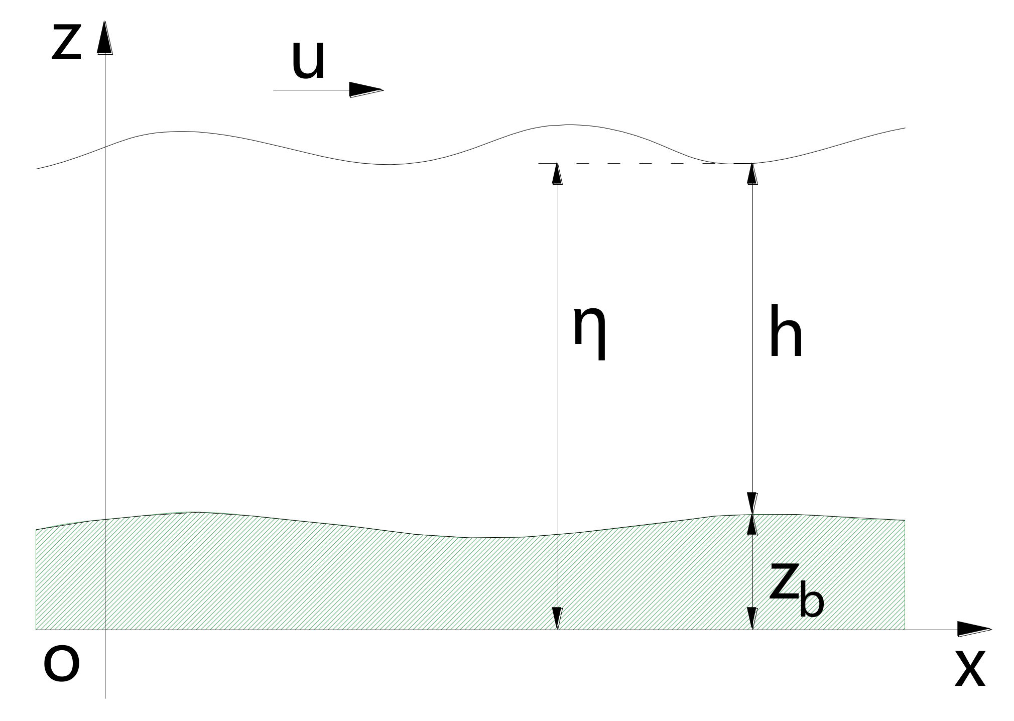
When the vertical velocity and displacement of water surface is sufficiently small compared with the frequency of water waves (Figure 1), the governing equations of shallow water flows can be obtained by integrating the Navier–Stokes equation over depth by assuming a hydrostatic pressure distribution, as well as a uniform distribution of the horizontal velocity in the vertical direction and a small bottom slope. Neglecting the diffusion term due to viscosity and turbulence, the Coriolis term, and the surface shear stress term, SWEs can be expressed in a vector form:
where denotes time; and are Cartesian coordinates in the horizontal plane; represents the vector of conserved variables; and are the vectors of convective fluxes in and directions, respectively; is the flux tensor; and denotes the source term, which can be further divided into the bed slope source term and friction source term . These vectors are expressed as:
where represents water depth; and are depth-averaged velocities in and directions, respectively; is gravitational acceleration; is the bottom elevation relative to the datum plane, as demonstrated in Figure 1; and is the bed roughness coefficient evaluated by:
where n denotes the Manning coefficient.
Nontrivial steady solutions to SWEs are physically prevalent in shallow water phenomena as the time partial derivative term in Equation (1) vanishes and the SWE is deduced to . One of the most important and interesting steady solutions is the “lake at rest” one:
If the water surface remains constant over the domain and the flow velocities vanish, the bed source term and the flow depth gradient term in Equation (2) reach balance automatically. However, it is not always the case, because these two terms are discretized separately. Numerical difficulties may arise in situations when they should exactly balance with each other [28].
The flux Jacobian matrix of SWEs (Equations (1) and (2)) is:
where and are, respectively, two components of the unit vector in the and directions.
The eigenstructure of the flux Jacobian matrix is:
where and represent the right and left eigenvector matrices, respectively, and is the diagonal matrix of the eigenvalues of , given by:
where , , and denote three eigenvalues of and , , and . Obviously, these three eigenvalues are all real and distinct from each other, provided the water depth is positive, so SWEs confirm strict hyperbolicity.
3. Numerical Method
3.1. FVM on Triangular Grids
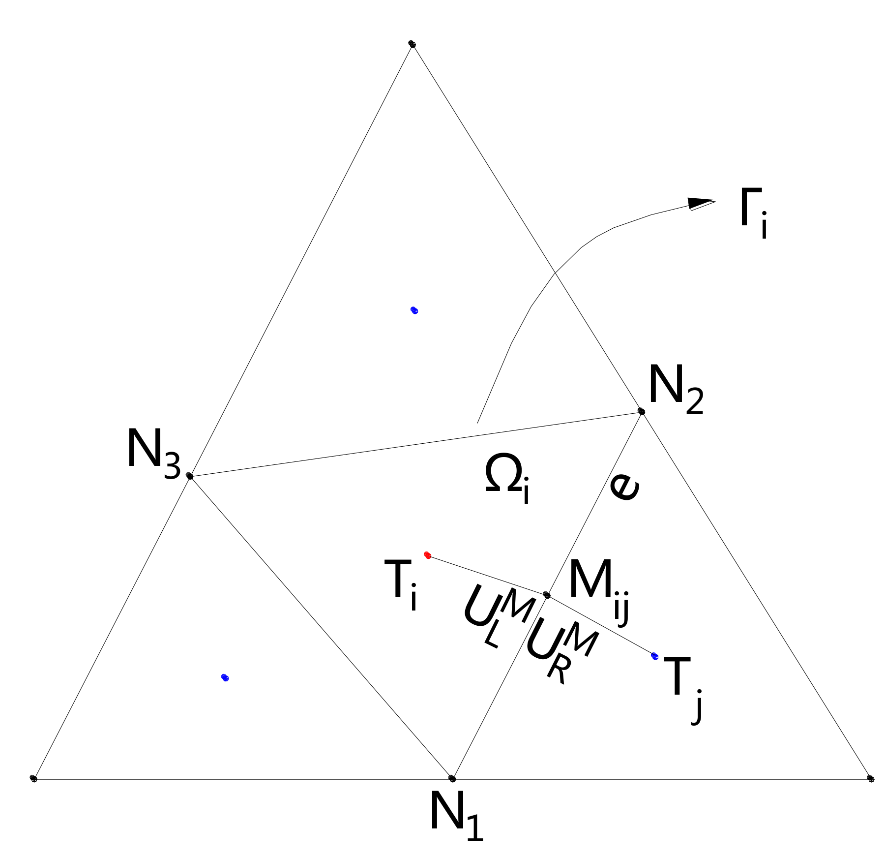
Two-dimensional grids used for numerical schemes range from structured to highly unstructured. Unstructured triangular grids are adopted in this work for their extreme flexibility with complex flow fields. Values of flow variables are stored at cell centroids, and a piecewise constant distribution is assumed over the computation domain, which conforms to the CCFV scheme. As illustrated in Figure 2, denotes the centroid of cell i; , and are three nodes anticlockwise around ; j is one of the three neighbors of cell i sharing a common edge e; and is the midpoint of edge e where a local Riemann problem is constructed.
SWEs (Equations (1) and (2)) can be integrated over cell i:
where is the control volume, as shown in Figure 2.
Applying Gauss’s divergence theory to the spatial derivative term in Equation (8) yields:
where and denote, respectively, the area and boundary of cell i and represents the cell-averaged values of conserved variables at a given time.
Assuming a uniform distribution of fluxes along each edge, which are equal to the values at the midpoint of the edge, the surface integral in Equation (9) is redefined and a semidiscrete scheme is given by:
where N is the number of edges for cell i; is the length of edge k; and is the outward normal flux vector across edge k and can be estimated with the help of Riemann solvers. The expression of is:
where and are two components of the unit outward normal vector at the midpoint of edge f.
3.2. Approximated Riemann Solver
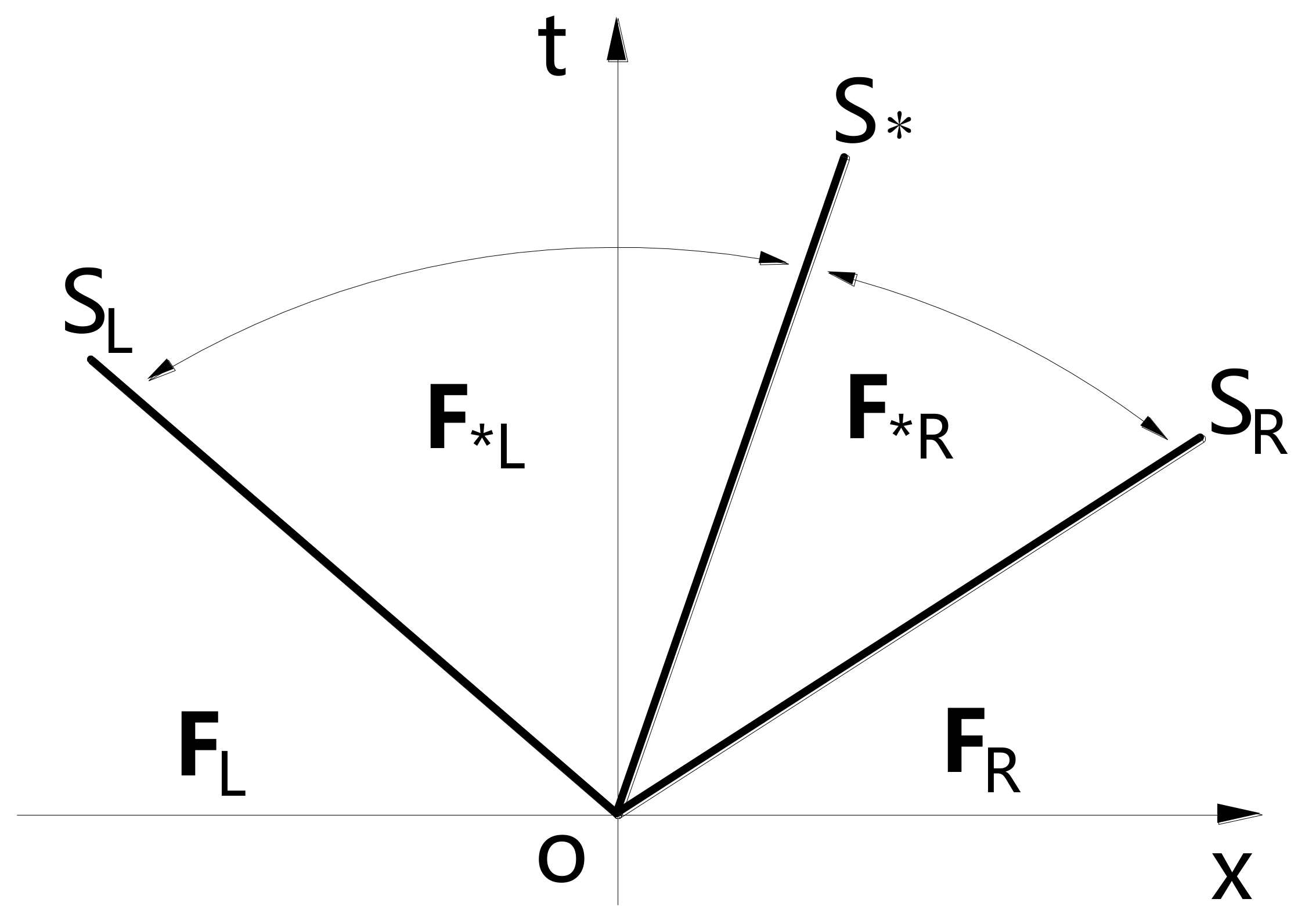
The Harten–Lax–van Leer–contact (HLLC) approximated Riemann solver [29] is used in the construction of numerical fluxes. Other solvers can be adopted as well, but are not presented in this work. The HLLC approximated Riemann solver restores the missing rarefaction wave by some estimates, for instance, using the Roe average velocity as the speed of the middle wave, which is very efficient compared with the exact Riemann solver, while behaving robustly. The numerical flux vector normal to the considered edge is:
where and are the Riemann states to the left and right of the considered edge; can be calculated by Equation (11) using as the independent variable, and the similar operation for ; and are the left and right wave speeds; denotes the contact wave speed; and and are the numerical flux vectors to the left and right of , as shown in Figure 3.
The values of the wave speeds , and can be evaluated by [30]:
where the superscript denotes the quantities of flow variables normal to the considered edge, for example, , and and represent, respectively, the water depth and flow velocity normal to the considered edge in the star region and can be evaluated based on the two-rarefaction assumption [31]:
and can be calculated in a simplified version based on the HLL approximated Riemann solver [32]:
where the superscript denotes the quantities of flow variables tangential to the considered edge, for example, , and and are two components of the numerical flux vector calculated by the HLL approximated Riemann solver:
where , and are all column vectors with two components, , , and , respectively.
3.3. Treatment of Source Term
Simulating shallow water flows over irregular topography demands appropriate treatment of the bed slope source term to achieve well-balanced property. A bed slope source term discretization method developed by Hou [33] is adopted in this work. A brief introduction is given below.
The integral form of the bed slope source term in cell i can be rewritten as:
Integrating Equation (17) with the first-order time marching scheme of SWEs yields:
where the bed slope source term has been transformed into the sum of fluxes across the edges, expressed as:
where and are, respectively, the water depth and bottom level at the centroid of cell i; and and represent the reconstructed values of the water depth and the bottom level obtained by Equations (43) and (41), respectively.
With respect to the friction source term, the splitting implicit method proposed in [20] is adopted in this work to properly handle the friction source term:
where the continuity equation is omitted and is the implicit friction source term expressed by:
where and are limited by a criterion:
3.4. Time Integration Scheme
To achieve second-order accuracy in time, the two-stage Runge–Kutta time integration scheme is adopted in this work to update solutions to the new time step. The detailed description of this time integration scheme is given by:
where
where is evaluated by:
Stability Criteria
The time step used in an explicit time integration scheme must be limited by some stability conditions, otherwise errors could be produced and convergence difficulties could arise. The Courant–Friedrichs–Lewy (CFL) condition is used in this work to estimate the time step:
where CFL is the Courant number, specified in the range of (0, 1] (CFL = 0.5 is used in this work); R denotes the minimum distance from the centroid to the boundary of cell i; u, v and h are the values of flow variables located at the cell centroid; and is the total number of cells.
3.5. Second-Order Spatial Reconstructing and Limiting Method
To achieve high-order accuracy in space, the MUSCL scheme introduced by Van Leer [21] has been a widely used numerical technique for its inherent simplicity and adaptation capacity [22]. Numerical results show that the MUSCL scheme can effectively reduce diffusion in the original Godunov-type scheme [34], leading to improved resolution of water surface where large gradient or discontinuity occurs. Specifically, there are two types of MUSCL schemes, depending on how the values of flow variables are reconstructed: the monoslope and multislope MUSCL schemes. The primary difference between these two schemes is that the former calculates only one vectorial slope per cell, whereas the latter calculates three specific scalar slopes for each edge per cell. It is notable that the monoslope MUSCL scheme involves an additional step for selecting the best limiter [35]. Correspondingly, for the multislope MUSCL scheme, scalar slopes are calculated in the same loop of evaluating numerical fluxes, which apparently leads to a more straightforward and efficient scheme. The multislope MUSCL scheme appears to be more robust when dealing with complex shallow water problems and more accurate than the monoslope one [34]. Moreover, the edge-based limiters chatter far less than the cell-based limiters, and better converging performance can be achieved. A review of these two schemes is presented below. Furthermore, a novel multislope MUSCL scheme is detailed.
3.5.1. A Review of Monoslope MUSCL Scheme
The basic idea of the monoslope MUSCL scheme is briefly reviewed in this subsection by introducing the limited central difference (LCD) scheme [27], which is probably the most widely used MUSCL-type scheme to date. The LCD scheme consists of two stages: the reconstructing stage and the limiting stage. As illustrated in Figure 2, U denotes one of the components of the flow variable vector U and denotes the direction vector from to . The value of can be extrapolated from the centroid with a limited slope:
where represents the gradient of U in cell i, which can be evaluated by neighbors’ values with the help of the least squares method [36] or Green–Gauss method [37]; denotes the limiting function:
where the expression of can be found in [27].
3.5.2. Review of Multislope MUSCL Scheme
A recent representative multislope MUSCL scheme proposed by Touze [34] is introduced in the following, which essentially extends the original multislope MUSCL schemes [17,22], and based on that a review of the multislope MUSCL scheme is presented.
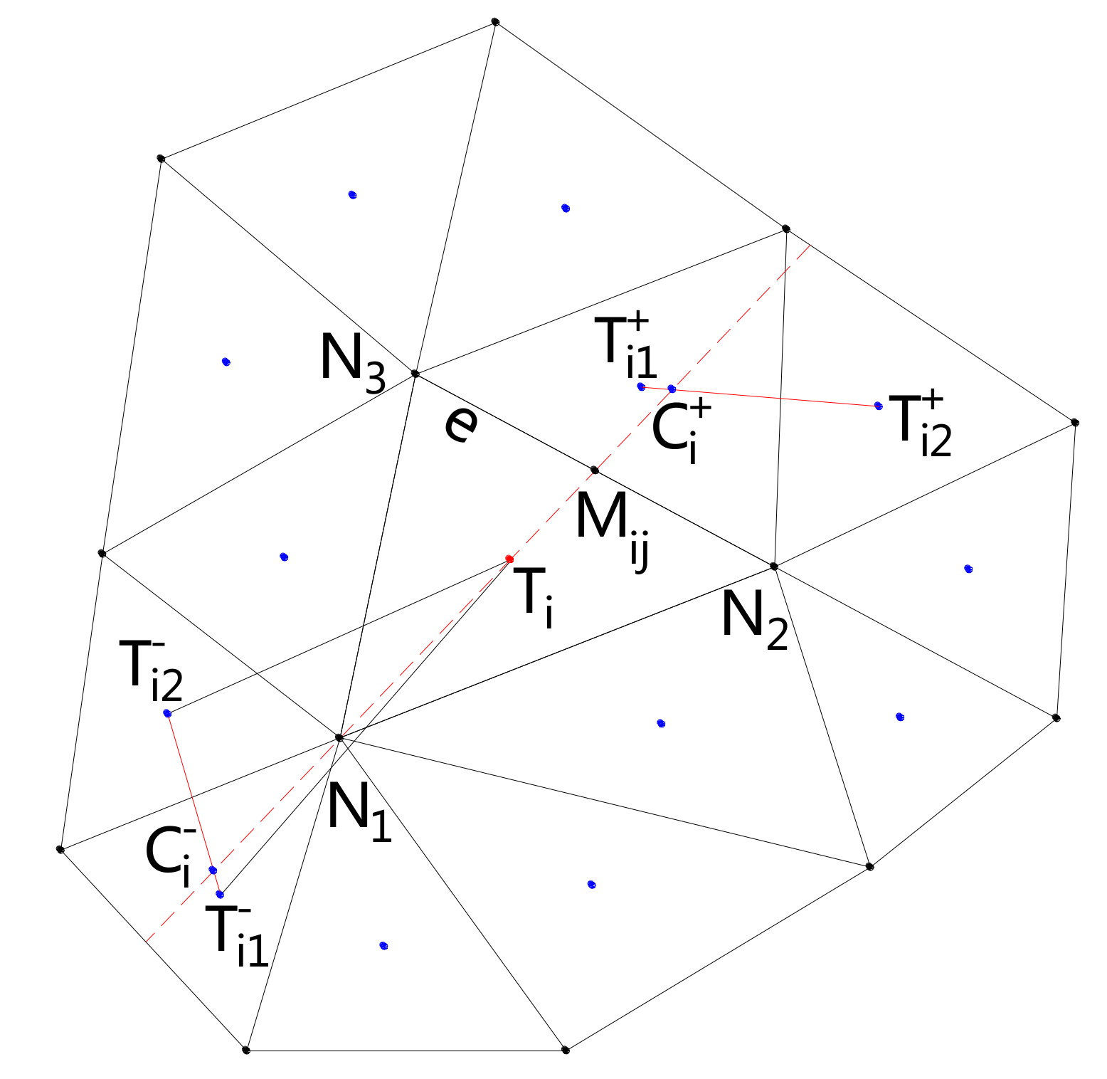
A wide stencil is illustrated in Figure 4, which consists of cell i and its neighbors sharing at least a common node; and represent the two most upwind neighboring centroids relative to in the direction of ; and represent the two most downwind neighboring centroids relative to in the direction of ; and and are the intersections of with and , respectively. These two points are exactly the upwind and downwind points relative to in the direction of . The highlight as well as the challenge of Touze’s scheme is to construct the upwind and backwind points and , where the values of flow variables are used to calculate the upwind and downwind slopes, and . These two slopes are then employed as arguments in the limiting function to calculate the directional scalar slope for the considered edge.
To sum up, the principle of the multislope MUSCL scheme is to construct the upwind and downwind slopes. Despite the merits of better robustness, higher accuracy, and better converging performance compared with the monoslope scheme, the drawback of the multislope MUSCL scheme is also obvious: a wider stencil is necessary for evaluating the slopes, which makes the scheme not straightforward because of the procedure for selecting the most upwind and downwind points, so additional computation cost is inevitable. Hence, a more straightforward and efficient numerical scheme is proposed in this work that can efficiently avoid the complicated procedure, while at the same time, the merits of the multislope MUSCL scheme are perfectly inherited.
3.5.3. A Novel Multislope MUSCL Scheme
Based on the basic idea of the multislope MUSCL scheme proposed by Touze, a novel multislope MUSCL scheme equipped with the edge-based Van Albada slope limiter, which takes into account the geometric characteristics of triangular grids, is presented below.
Considering the CCFV scheme adopted in this work, the first thing to calculate is the values of flow variables located at cell nodes, which can be evaluated from neighboring centroids with the method of inverse distance weighting (IDW) [38]:
where denotes the value of the flow variable U located at ; is the total number of neighboring cells of ; denotes the value of the flow variable U located at , which is one of the neighboring centroids of ; and denotes the weighting coefficient related to the distance between and :
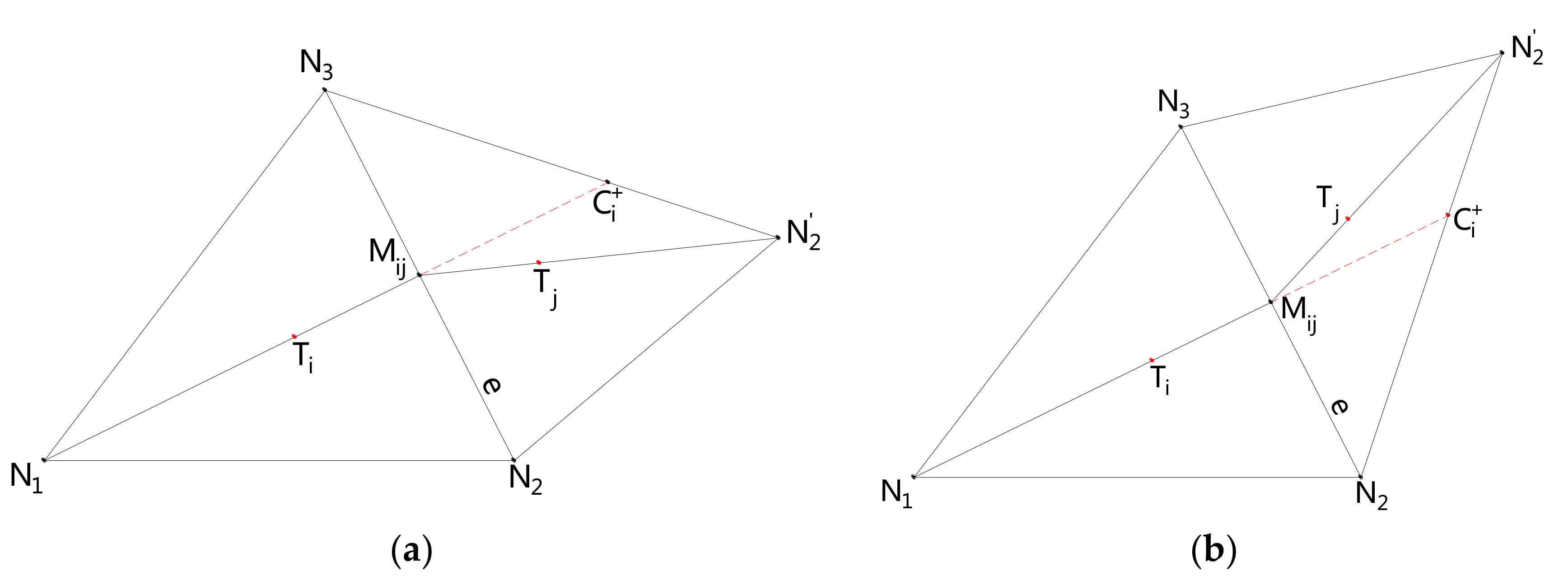
Two different cases should be taken into consideration, as shown in Figure 5. The criterion is straightforward and independent with the shapes of triangular grids:
where the coordinates of the midpoint can be obtained by those of and . In case (a), the intersection of and cell j locates at the edge , whereas in case (b), the intersection locates at the edge . For the sake of clarity, the following steps are only for case (a).
Similar to Touze’s scheme, cell j can be seen as the most downwind cell relative to cell i, and the intersection can be regarded as the downwind point in the direction of . The value of located at is evaluated by:
where and denote the weighting coefficients with respect to the neighboring nodes of , that is, and in case (a), which can be evaluated by:
As shown in Figure 5, the line connecting and also passes through the node , which is selected as the upwind point in the direction of . Considering that the value located at is known, the upwind and downwind slopes for the considered edge are almost ready and given by:
where denotes the value of U located at .
The modified Van Albada limiting function (Equation (35)) [17,26,39] is employed here to turn the upwind and downwind slopes into a limited slope, which is then used to calculate the left and right Riemann states:
where ranges between 0 and 1 and is defined by Equation (36), and and denote, respectively, the upwind and downwind slopes; and
where e is a constant used to prevent division by zero and is adopted in this work.
The flow states on the considered edge, for example, the left flow state of the flow variable U located at , can be calculated by:
Similarly, the flow states on the other edges can be obtained by repeating the above steps.
In order to preserve the C-property, only , , and are reconstructed [14], which gives rise to the left and right Riemann states, i.e., , , , , , , and . The bottom level and velocity components in x and y directions are subsequently obtained by:
A criterion proposed by Hou [33] is adopted here to identify problematic cells next to the wet-dry interface:
where and denote, respectively, the water depth and bottom level to the left of the considered edge; and denote, respectively, the water depth and bottom level at the centroid of cell i; and is the threshold of water depth used to distinguish wet and dry cells, and [40,41] is adopted in this work.
3.6. Treatment of the Wet-Dry Interface
The second-order MUSCL scheme degenerates to first-order accordingly once the criterion in (Equation (39)) is met, that is, the left and right Riemann states are respectively constant with cell-averaged values. By doing so, abnormal reconstructed values are effectively avoided. Furthermore, numerical schemes integrated with an appropriate Riemann solver can properly handle the transience of flow state from wet to dry zones, as long as the topography is horizontal or slowly varying. However, realistic topography is quite inhomogeneous: adverse or abruptly steep slopes are common in cells next to the wet-dry interface. Water depth gets smaller and smaller as flow advances, leading to extremely high velocity, which is unacceptable for simulation. Hence, particular numerical techniques must be used in the representation of wet-dry interface. The classic hydrostatic reconstruction method [14] and the local bed modification technique [18,42] are combined in this work to deal with the wetting and drying problem, stated as follows.
A single value of the bottom level at the common interface is defined by:
Considering those sensitive cells over adverse slopes, a bed modification strategy is carried out to hold the stopping flow condition:
The water surface elevation on the right side of the common interface is modified accordingly:
Then the left- and right-side water depths are reevaluated as:
After these steps, is obtained at the wet-dry interface, which is in agreement with the equilibrium condition proposed by Brufau [42]. The water surface elevation over adverse slopes is equal to ηL, so spurious flow motion is effectively prevented and the well-balanced property is perfectly preserved.
3.7. Boundary Conditions
Boundary conditions provide information about how the water along boundaries responds to external disturbances. In order to achieve an optimal simulation for shallow water flows, an adequate treatment of boundary conditions should be considered. Basically, there are two approaches to implementing boundary conditions: using ghost cells and directly calculating fluxes across boundaries. In this work, the latter is adopted by solving Riemann problems along boundaries. Boundaries need to be divided into two distinct sections: the liquid boundary and the solid boundary. The former can be further subdivided into four different cases.
3.7.1. Liquid Boundary
There are four cases to take into account for the liquid boundary, depending on the flow velocity normal to boundaries and the local Froude number , expressed as [43]:
Supercritical inflow ():
Supercritical outflow ():
Subcritical inflow ():
Subcritical outflow ():
In order to calculate the numerical fluxes through boundaries, a reverse transforming operation is applied to velocities as soon as and have been obtained:
where is equal to along boundaries.
Once the flow states to the right of boundaries are obtained, a local Riemann problem can be set up and then settled by the HLLC Riemann solver, where the left flow states of the Riemann problem can be evaluated by averaging those at the two adjacent nodes located on the boundary edges, since they have been obtained from neighboring centroids with the IDW method.
3.7.2. Solid Boundary
Normal velocity is ignored in this situation, and the value of water depth is taken from the internal computational domain, that is, . The normal fluxes at the midpoint of the considered edge along solid boundaries can be evaluated by a simplified form of Equation (11):
4. Verification and Application
4.1. Stationary Flow with Wet-Dry Interface
A well-balanced scheme should correctly compute the solutions to a steady state and maintain the stationary state throughout the simulation for a quiescent shallow water problem. A simple test is employed here, as also used in [44,45], to verify the well-balanced property of the new scheme. A hump is defined in an 8000 m long square basin with topography given by:
where the solid boundary condition is imposed on vertical walls. The initial water surface is given by 1000 m, so the hump is partly submerged. The computational domain is discretized into 15,360 Delaunay triangles, and the simulation is run until t = 1500 s.
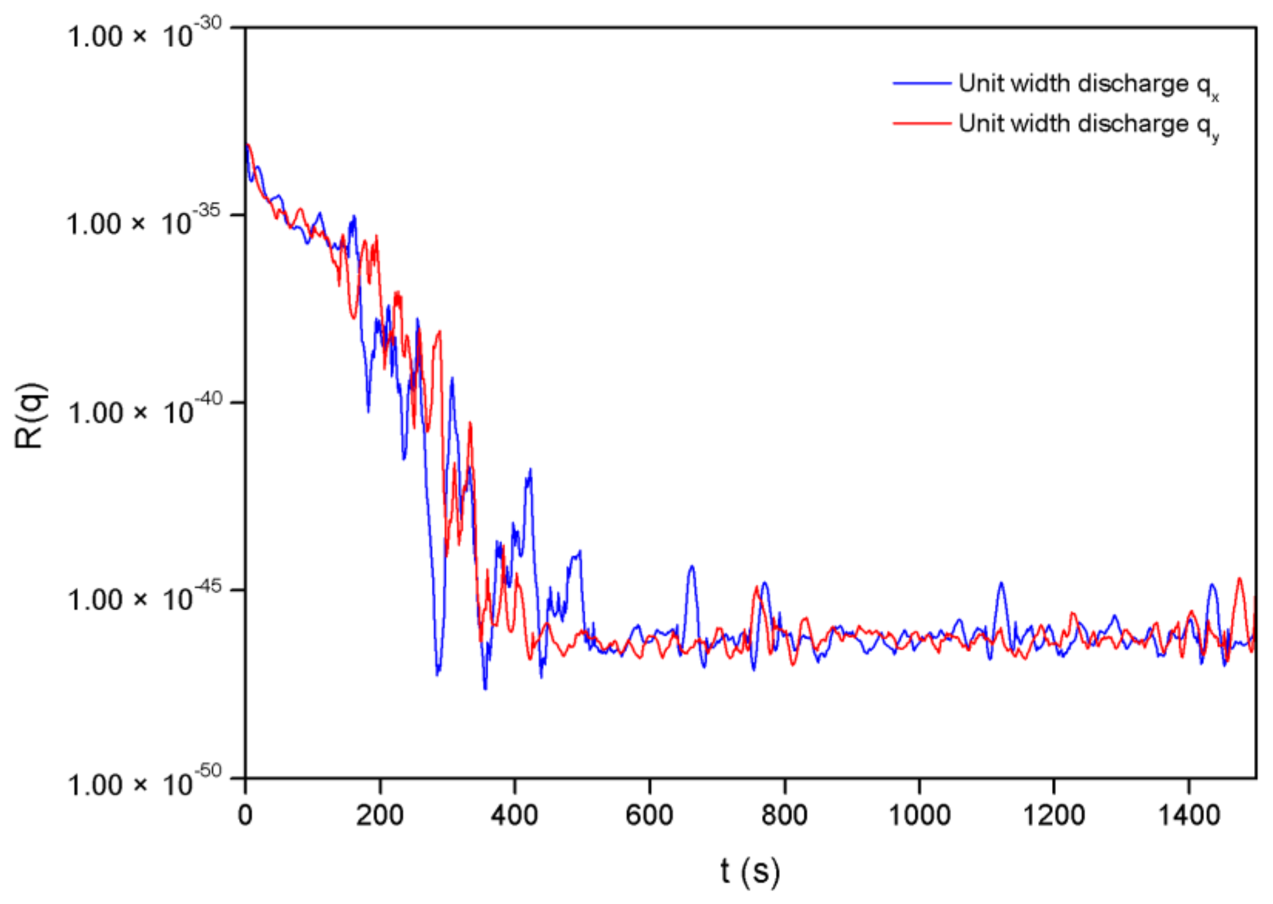
A variable is defined to quantify the global relative error of solutions following Zhou [45]:
where and denote, respectively, the vectors of flow variables at time level n and n − 1 for cell i.
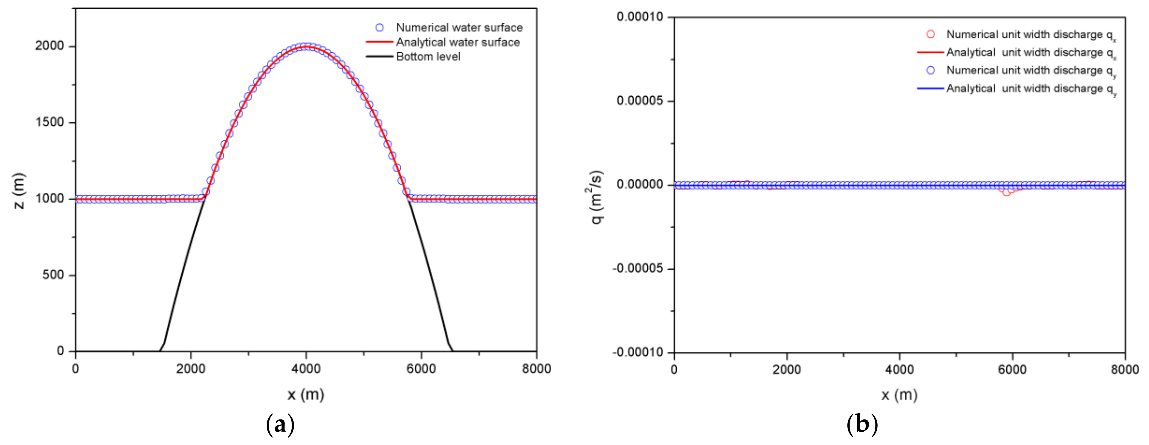
Figure 6 gives the numerical results of water surface and unit width discharges in x and y directions. The stationary state is visible at the end of the simulation, since the numerical water surface elevation almost coincides with the analytical result. With regard to the numerical unit width discharge, a little wriggle can be observed in Figure 6b in terms of . As a matter of fact, the global relative error is quite small, as illustrated in Figure 7, where both and hold rather small values (lower than ) throughout the simulation; such a result is acceptable and the well-balanced property is well preserved.
4.2. Potential Flow over Uneven Bottom
As proposed by Ricchiuto [46], the steady flow with divergence-free velocities over uneven bottom is simulated here to verify the capacity of the new scheme to preserve monotonicity and converge to steady-state solutions in the presence of irregular topography. This test case was performed in a smooth square domain, , where the velocity field is obtained by the harmonic function:
The velocities in and directions are expressed as the partial derivatives of :
The analytical water depth and bottom level of the test case are calculated by:
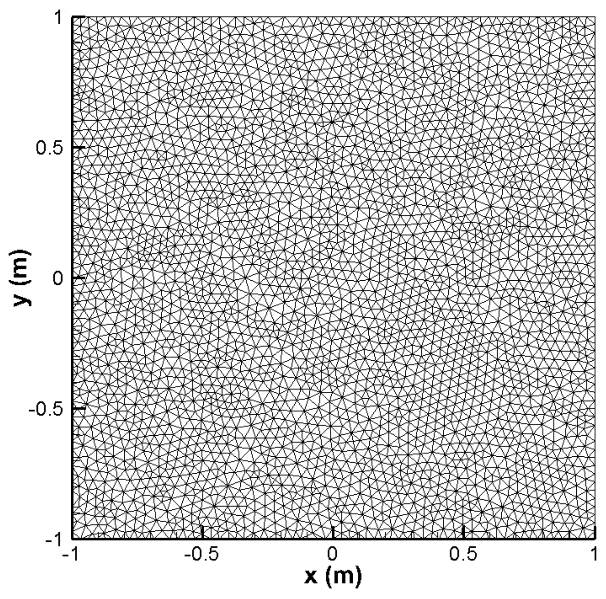
Considering the Froude number inside the computational domain is always less than 1, the north and south edges are used as subcritical inlet boundaries and the east and west edges are used as subcritical outlet boundaries during the simulation. The computational domain is discretized into 6341 Delaunay triangles, as shown in Figure 8. The simulation is run with the initial conditions calculated by Equations (53) and (54) until t = 50 s.
Figure 9a,b illustrate, respectively, the numerical results for water depth and flow velocities computed at the end of the simulation by the new scheme proposed in this work. It can be observed that the new scheme is able to converge to the steady-state results in terms of water depth and flow velocities on Delaunay triangles at the end of the simulation. The contours of the water depth are symmetric about two diagonal lines of the computation domain, which agrees well with the analytical results, since the analytical water depth (Equation (54)) matches a hyperbolic-paraboloid distribution. In addition, the velocity field of this test is also well predicted at the end of the simulation, because the distribution of flow directions is very regular, as shown in Figure 9b, and obviously there are no unphysical high velocities inside the computational domain. The numerical results confirm that monotonicity in the limitation procedure is guaranteed, and the new scheme can achieve convergent results in the case of irregular topography and nonzero velocities.
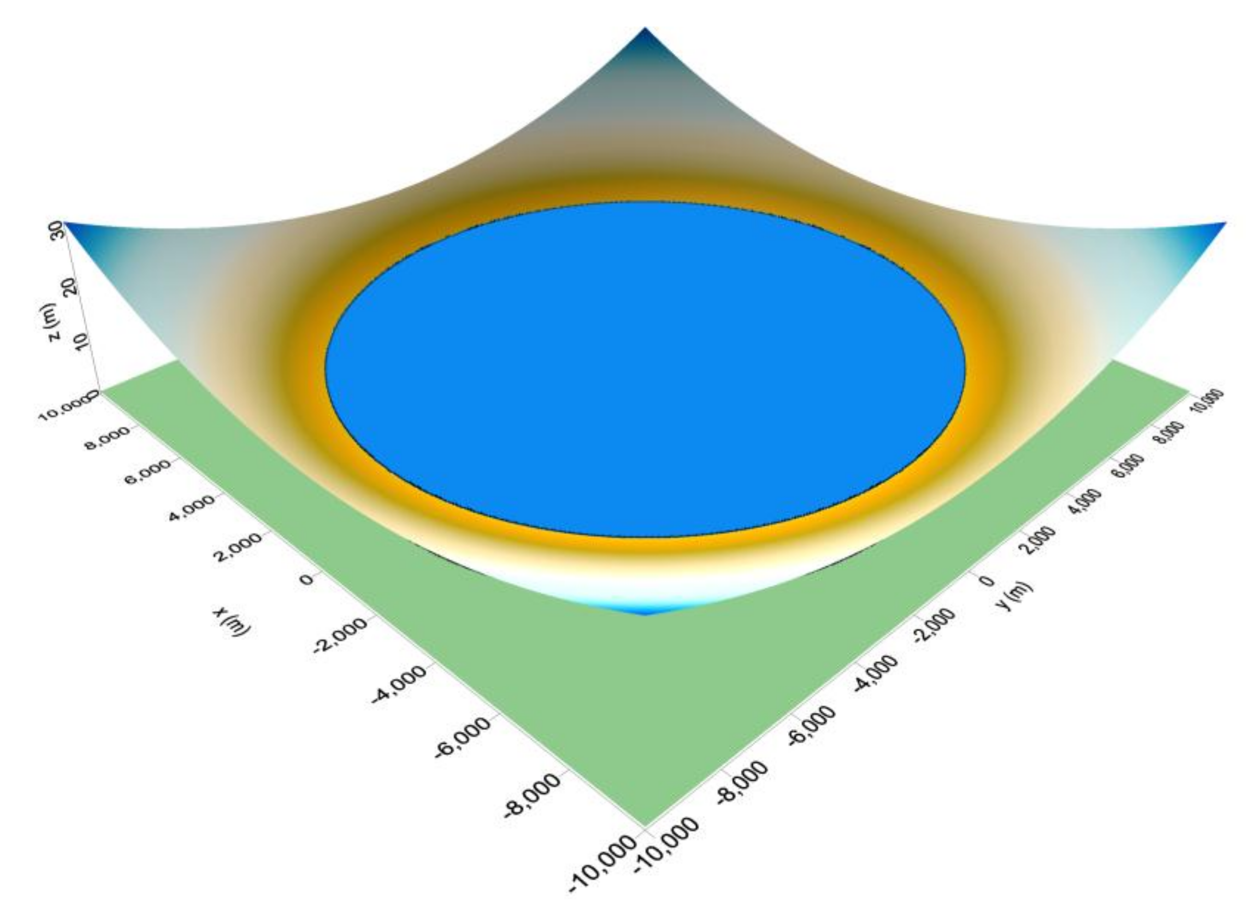
4.3. Water Sloshing in a Parabolic Basin
The test proposed by Thacker [1] on water oscillation in a smooth 2D parabolic basin, as illustrated in Figure 10, has been a classical benchmark for evaluating the accuracy of and capacity to deal with the wetting and drying problem of numerical schemes [17,47,48] and is employed in this subsection. There is a parallel test, developed in [49], that takes the effect of friction source term into consideration and is widely used by many other researchers [33,50]. The bottom level of the parabolic basin is defined by:
where denotes the water depth at the center of the basin and denotes the distance from the center to the shoreline with zero elevation; the analytical solutions of velocities and water depth are:
where σ is a constant denoting the amplitude of the water motion and ω denotes the frequency of the water motion and is calculated by ; values of the parameters used in this test are , , , , and .
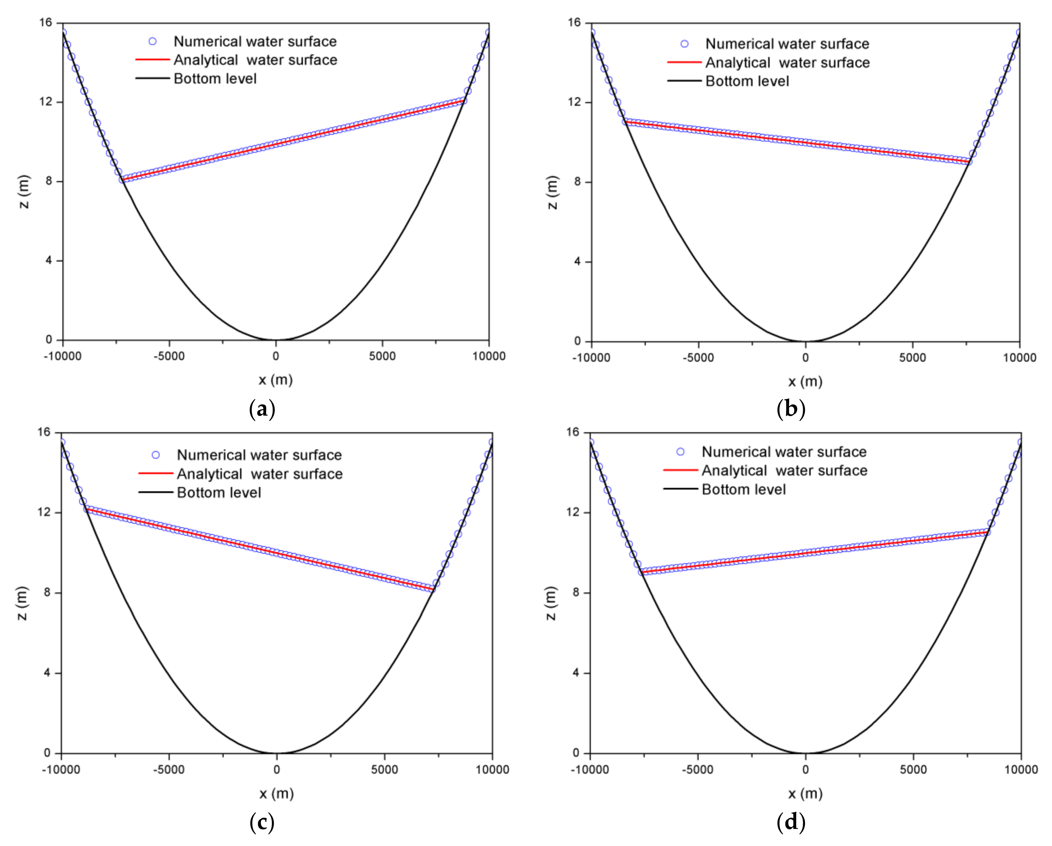
The computational domain is discretized into four scaled meshes with sizes of ∆L = 55.18 m, 108.49 m, 138.58 m and 205.02 m, where ∆L is the averaged grid size, calculated by . For each scaled mesh, the number of Delaunay triangles is 128,418, 33,038, 20,516 and 9304, respectively. The analytical solutions at t = 0 calculated by Equation (56) are used as the initial conditions. In addition, the solid boundary condition is employed in this test. This simulation is carried out for three periods, i.e., t = 10,800 s.
The comparison between the analytical and numerical results of water surface along the x-direction symmetric axis at t = T, T + T/3, T + T/2 and 2T + T/6 for the smallest scaled mesh is depicted in Figure 11. Compared with the analytical solutions, the numerical water surface and shoreline show good agreement with the exact results, meaning the new scheme can accurately capture the moving boundaries and handle the wetting and drying problem well. Moreover, two components of flow velocity at the point (−5000, −100) versus time are also depicted in Figure 12, demonstrating the difference between the numerical and analytical flow velocities, which is almost negligible.
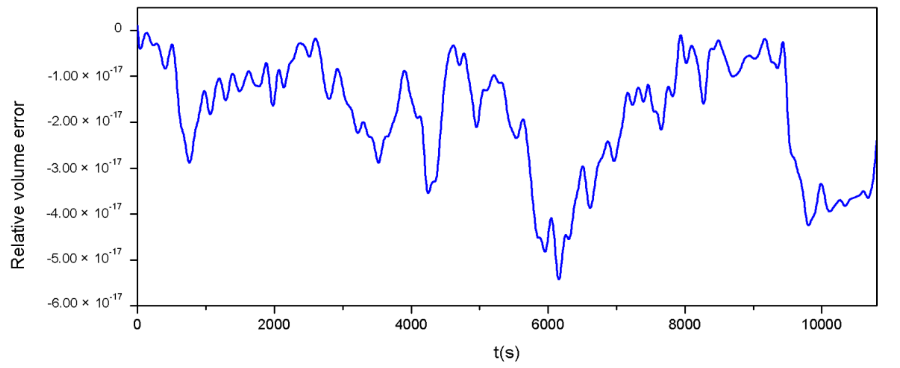
Figure 13 shows the relative error of the total volume of water during the simulation over time. The relative error ranges from to , indicating a rather small deviation from the initial total water volume, and the new scheme proposed in this work ensures mass conservation. The errors in and norms, reflecting the deviation between numerical and analytical solutions, are widely used to investigate the convergence performance of numerical schemes and are also used in this work. Water depth and two components of unit width discharge at t = 3T versus the grid size ∆L in logarithm scale are plotted in Figure 14. It is obvious that, for all flow variables, the convergence rate in errors in both and norms is greater than 1.6. The accuracy is acceptable, considering the second-order reconstruction procedure has been switched to first-order in some problematic cells near the wet-dry interface.
4.4. Steady Flow over Frictional Uneven Bottom
A two-dimensional steady-state flow over uneven bottom considering friction effects, originally proposed by Murillo [51] and also adopted in [7,10,52], is employed here to test the new scheme when perturbations by friction source term are involved. The analytical water depth and bottom level satisfy Equations (57) and (58):
where a is constant and equal to 0.5, and
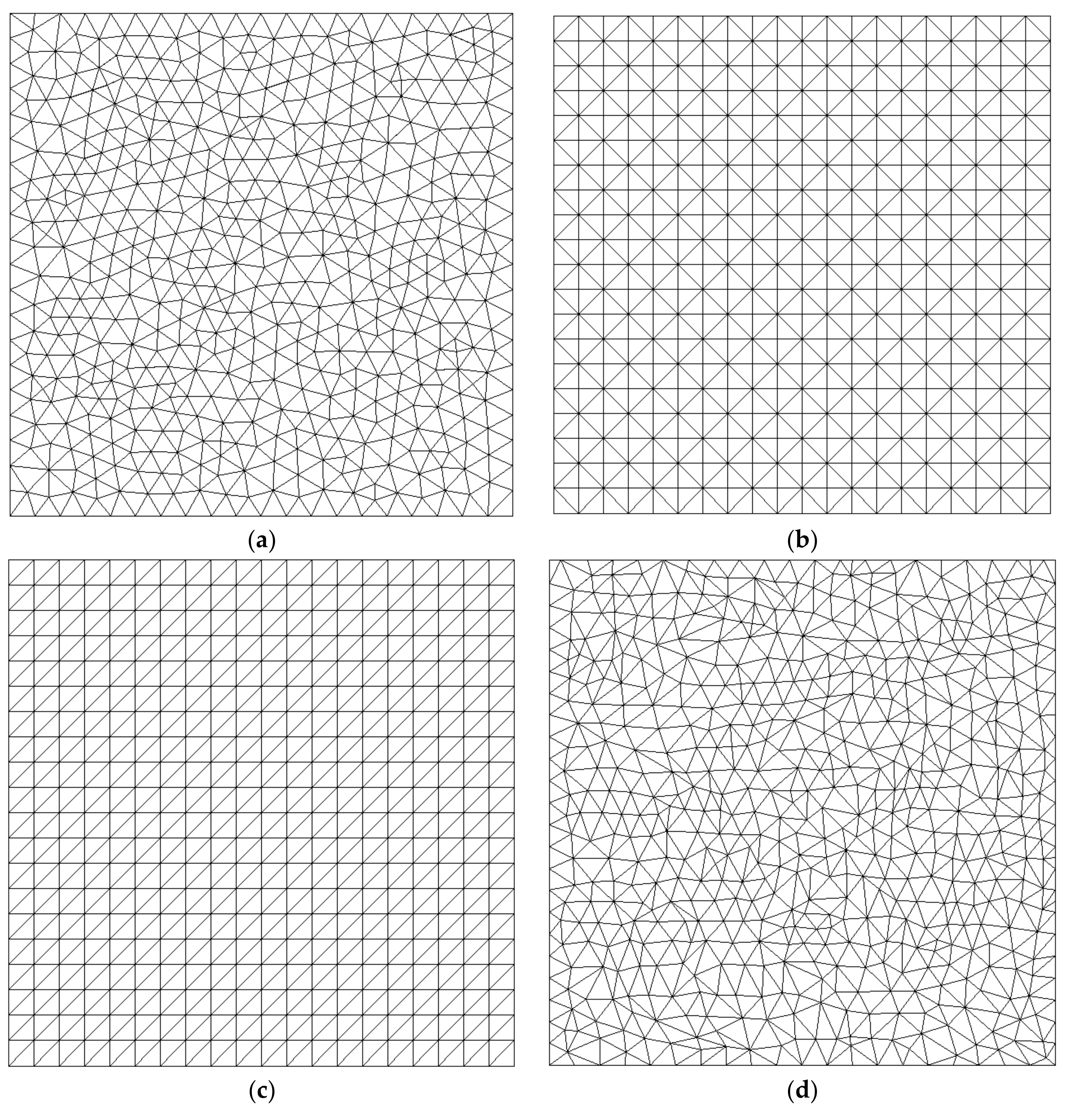
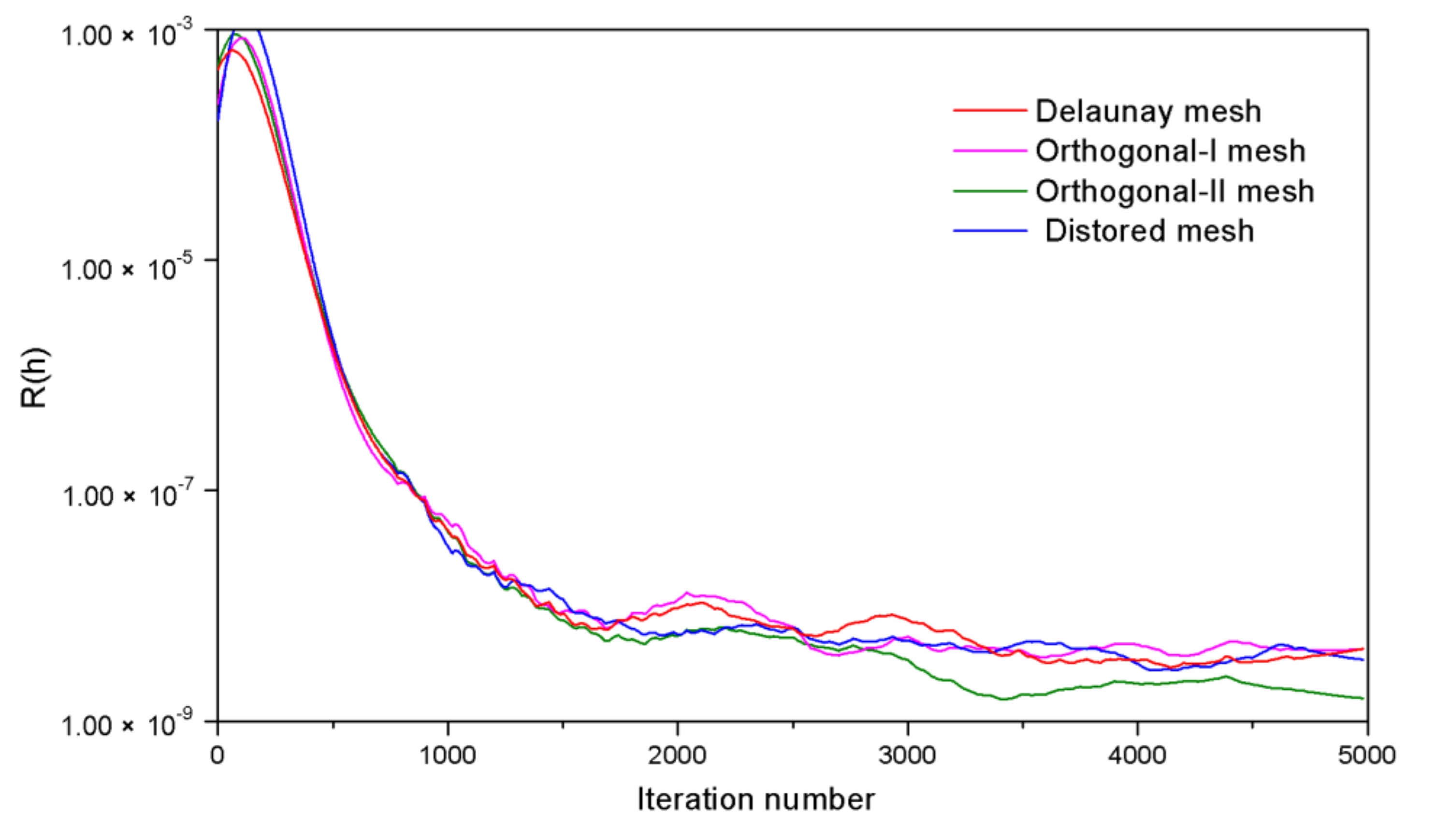
The computational domain is a square of 10 m. The unit width discharges in Equation (57) are assumed to be constant over the domain and . The Manning coefficient n throughout the domain is also a constant value taken as 0.03 . As shown in Figure 15, in order to study the adaptability and robustness of the new scheme on various irregular triangular grids, four types of triangular meshes are adopted in this simulation under the same initial and boundary conditions: the Delaunay mesh, the orthogonal-I mesh, the orthogonal-II mesh, and the distorted mesh. For each type of mesh, the number of discrete triangles is 1020, 800, 800 and 1111, respectively, and the number of nodes is 551, 441, 441 and 602, respectively. Once again, the global relative error defined in Equation (51) is employed in this test to quantify the convergent performance of the new scheme on different types of meshes, and is used as the criterion of convergent results.
Before computation, the initial water surface is set to zero and the still water condition is assumed over the domain. The constant unit width discharges are imposed on the west and south boundaries. The east and north boundary conditions are given by the water depth calculated by Equation (57). The simulation runs on four types of meshes for 25 s with a time step of 0.005 s.
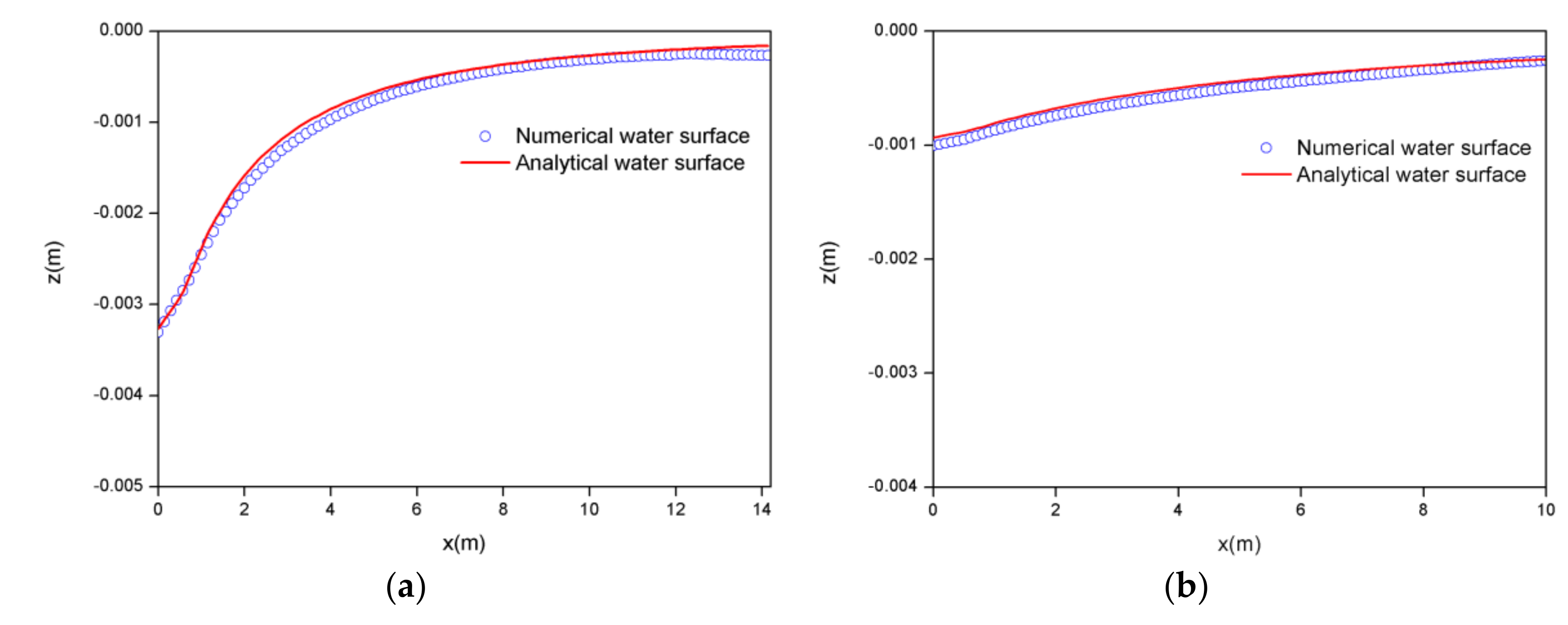
Figure 16 illustrates the global relative errors of the new scheme in terms of water depth for different types of meshes. In these four series of runs, the new scheme is able to converge to the steady state on all the mesh types at the end of the simulation (), even in the case of distorted mesh. Figure 17 displays the exact and numerical water surface at the end of the simulation along the diagonal section (Figure 17a) and horizontal-symmetry section (Figure 17b) of the computational domain on the distorted mesh. The comparisons show good agreement between the numerical and exact water surface even on the distorted grid (the difference is rather small, on the order of , for both recorded sections). In summary, this test demonstrates not only the validity of the friction source term treatment introduced in Section 3.3, but also the flexibility of the new multislope MUSCL scheme for irregularly shaped grids even in the presence of obtuse triangles.
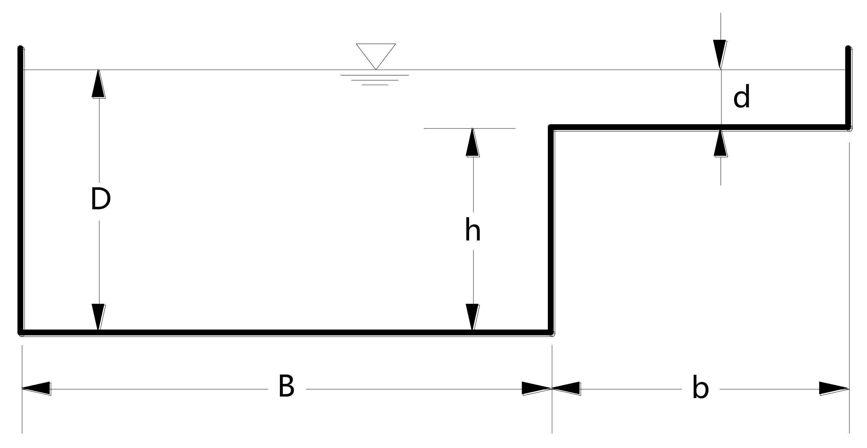
4.5. Flow in a Compound Channel
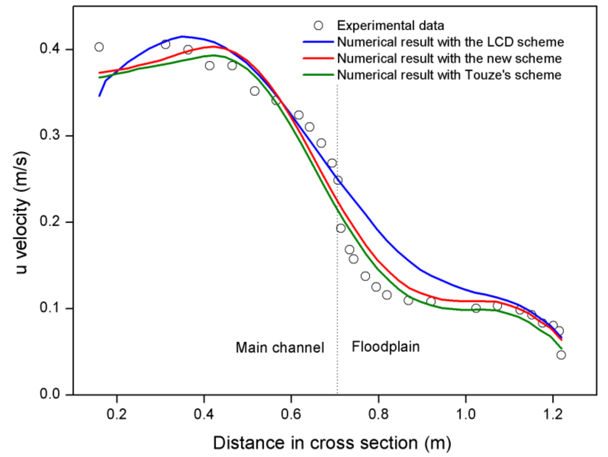
This test considers a commonly seen scenario in natural rivers: an asymmetric compound channel, as sketched in Figure 18. The physical experiment was conducted by Rajaratnam [53]. The channel was 18.3 m long and 1.22 m wide. The most significant characteristic of this channel was the distinctly different velocity distributions in the main channel and the floodplain, since a high step separates the main channel and the floodplain. Hence, the test simulated here is used to verify the capability of the new scheme to give an accurate prediction of different flow regimes caused by rapidly varying topography. For further comparison, three kinds of MUSCL-type schemes are used: the LCD scheme, Touze’s scheme, and the new scheme proposed in this work. Detailed parameters are listed in Table 1.
The computational domain is discretized into 17,164 Delaunay triangles. In order to sharpen the resolution of the topography equipped with an abrupt step, the computation domain is discretized using a longitudinal break line that exactly coincides with the line dividing the main channel and the floodplain in the horizontal plane. Triangles are distributed on both sides of the break line, resulting in the break line being discretized with triangle edges. The inlet boundary condition is given by a uniform velocity and the outlet boundary condition is given by a constant water surface elevation. In addition, the channel is supposed to be smooth, so the friction source term is negligible.
Figure 19 plots a comparison of the measured and simulated longitudinal velocities along the cross-section located 9.15 m from the inlet boundary. Three schemes can reproduce the dramatic decrease in streamwise velocity from the main channel to the floodplain. Correspondingly, a large gradient of streamwise velocity occurred at the interface of the main channel and the floodplain (the dotted line in Figure 19) due to an abrupt change of flow depth, consistent with observations in the published literature [54,55]. However, all the schemes exhibit some sort of numerical diffusion near the step, which leads the numerical results to deviate from the measured data. It means the two-dimensional shallow water model has an inherent limitation in dealing with this kind of case with sharp changing topography. It is also obvious that the numerical diffusions drag the flow momentum in the main channel to the floodplain and narrow the velocity gap between these two regions.
It is worth noting that compared with the LCD scheme, both multislope schemes perform better in capturing the large gradient of velocity, which is also stated by Delis [17] and Hubbard [27]. Moreover, slight differences can be found between the numerical results of Touze’s scheme and the new scheme proposed in this work. Similar accuracies are achieved by these two schemes and parallel large-slope capturing capabilities can be seen in Figure 19. However, the new scheme is more efficient than Touze’s scheme and the LCD scheme (4.353% and 4.976% runtime, respectively, saved in this test). This is because the new scheme avoids the addition loop for selecting an appropriate limiter in the LCD scheme and makes full use of the geometric characteristic of triangular grids, so the upwind point used for calculating the upwind slope is already available, which yields a more straightforward and efficient algorithm.
4.6. Flow in a Contracting-Expanding Channel over Uneven Bottom
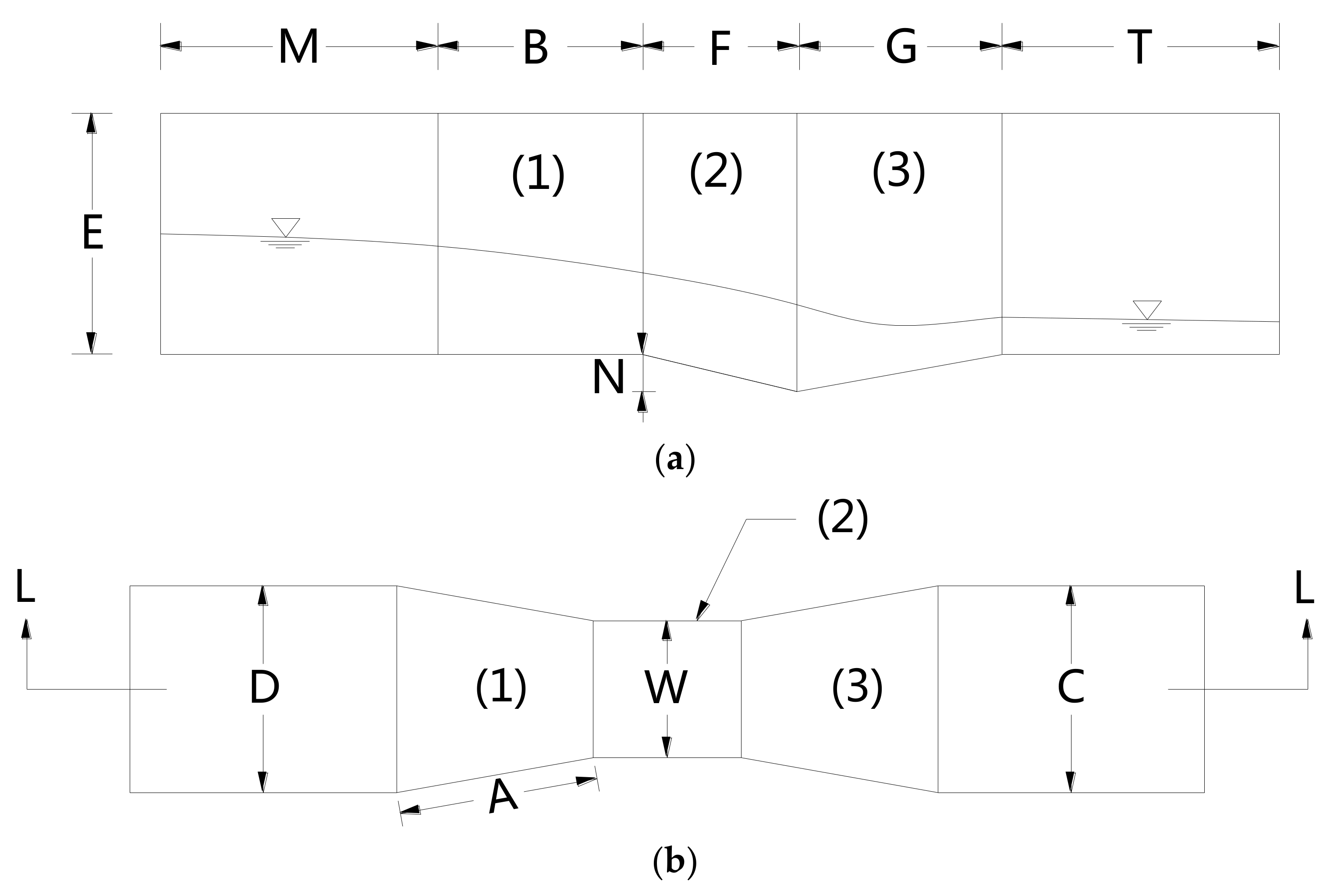
Parshall flume, a widely used device for field measurement in open channels, as shown in Figure 20, is employed to verify the applicability of the new scheme for varying flow regimes.
The corresponding experiment was initially conducted by Ye [56]. The flow discharge is 0.0145 m3/s at the inlet boundary, and the outlet boundary conditions do not influence the flow regime upstream. The water surface along the path is presented in Figure 21a. Zone 1 denotes the converging section where the cross-section contracts over a flat bottom to create a critical depth; zone 2 denotes the throat section over a sloping bottom where supercritical flow occurs; and zone 3 denotes the diverging section over an adverse slope bottom where the flow is supercritical. The flow regime along the flume varies from subcritical to critical and eventually reaches supercritical conditions downstream of the throat section. Complexly varying flow regimes present a great challenge to the accuracy and stability of the simulation. A robust numerical scheme should provide an accurate prediction for different flow regimes. The parameters of this experiment are listed in Table 2.
For numerical computation, the domain is discretized into 10,567 Delaunay triangles. The inlet boundary condition is given by u = 0.4 m/s and h = 0.12 m. The outlet boundary condition is not imposed since the supercritical flow regime. The initial condition is given by h = 0.05 m. In addition, the channel is supposed to be smooth.
Figure 21a depicts the distribution of water surface along the Parshall flume, including the numerical result computed by the scheme proposed in this work and the one provided in [56]. It can be seen that there is excellent agreement of the water surface profile between the numerical and measured results along the flume. Compared with the numerical results in [56], the numerical result in this work is obviously closer to the experimental data regardless of flow regime. This phenomenon is more pronounced for Ye’s numerical results in the supercritical flow regime downstream, where a large deviation from the experimental data occurs. Figure 21b illustrates the flow field of the numerical x-directional velocity calculated by the new scheme, which is shown to agree closely with the experimental data, although the velocity downstream is slightly greater than that of the experimental data. Since the frictional resistance will more or less affect the measured results, the difference of velocity downstream in the flume between the numerical results and measured data is acceptable. It is concluded that this new scheme can provide satisfactory solutions for varying flow regimes.
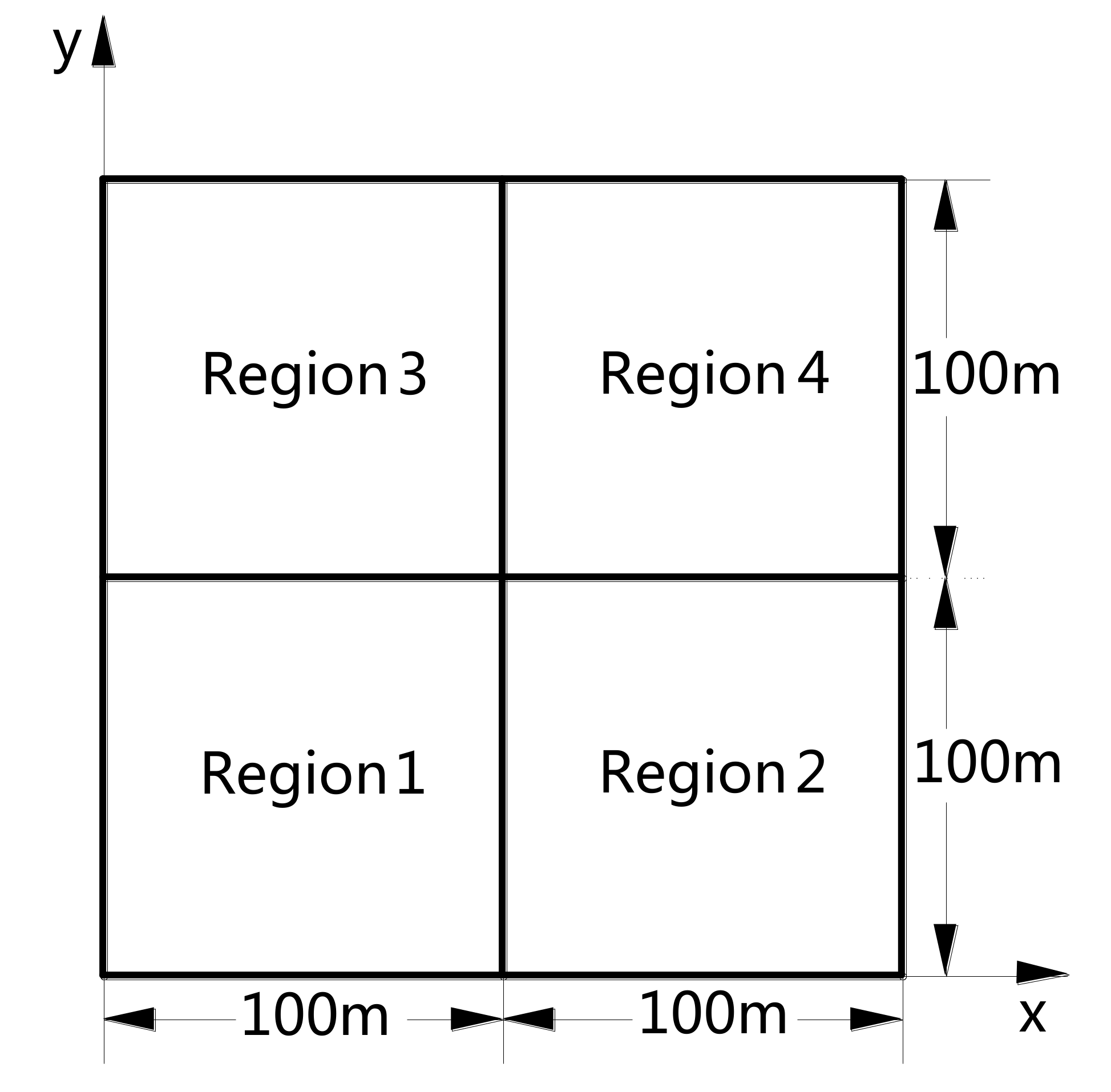
4.7. A Symmetric 2D Riemann Problem
The last test was proposed by Brio [57] and was widely adopted in other studies [17,58] to verify the shock-capturing capability of numerical schemes. This test aims to simulate the flow pattern arising from two streams intersecting at a straight angle over a frictionless square domain. As presented in Figure 22, the domain is divided into four subregions of equal size, where the bottom levels are all zero. The initial conditions are discontinuous and listed as follows:
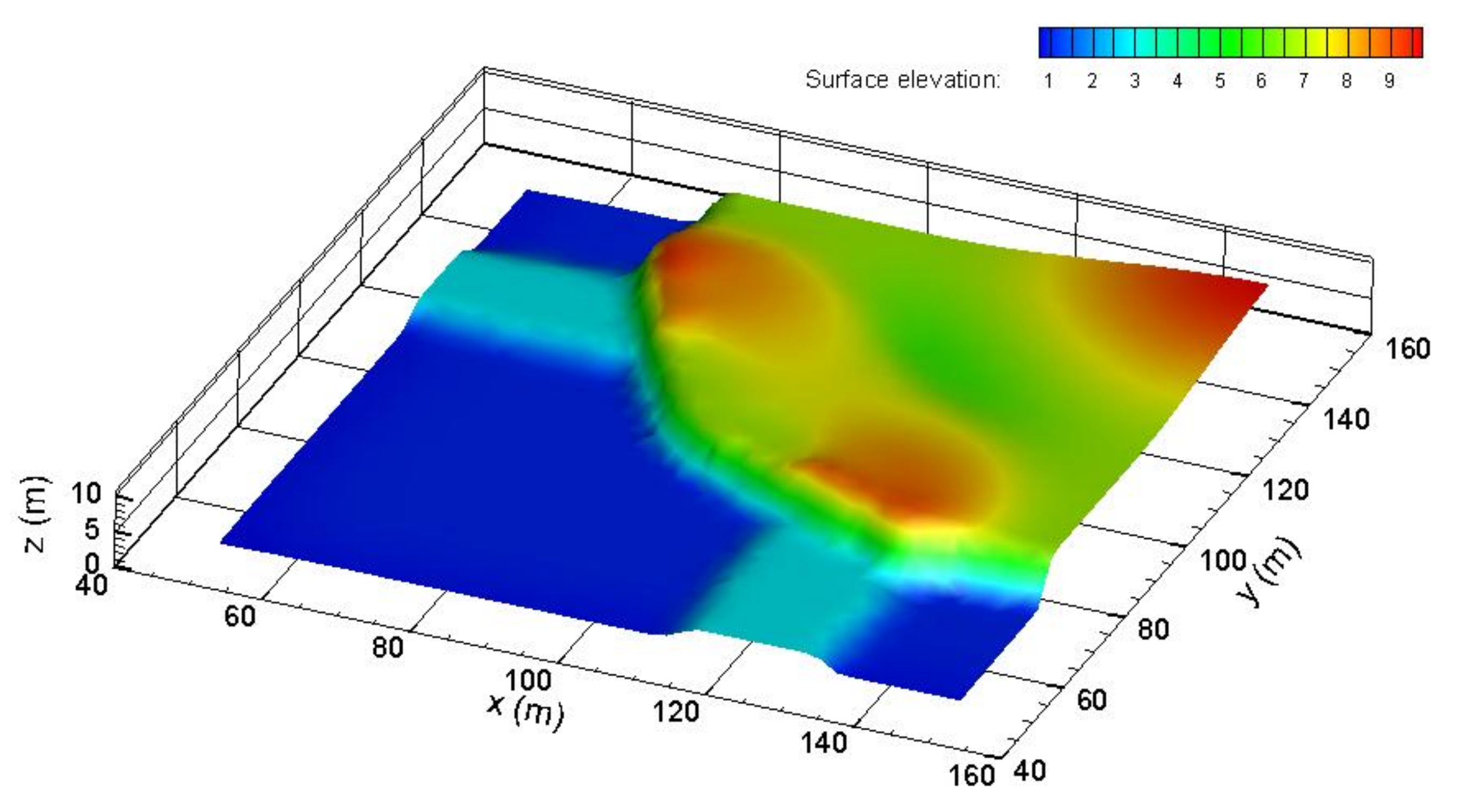
The interactions between different regions result in a complex two-dimensional wave pattern, which provides an excellent basis for verification of numerical schemes in terms of shock-capturing ability. The computational domain is discretized into 15,360 Delaunay triangles, and the new multislope MUSCL scheme is used to predict wave propagation. The initial flow conditions are given by the data in Table 3 and the boundary conditions are not prescribed, to avoid water reflection.
Figure 23 demonstrates the 3D view of the simulated water surface at t = 4 s in a square subregion . It is clear that the complex wave propagation pattern is well reproduced. The interactions between regions 1 and 2 yield two shock waves propagating along the x axis in opposite directions. A symmetric wave propagation pattern occurs as a result of the interactions between regions 1 and 3. The interactions between regions 4 and 2 yield a shock wave propagating along the negative y axis and a refraction wave along the positive y axis. A symmetric wave propagation pattern occurs as a result of the interactions between regions 4 and 3, where both a shock wave and a refraction wave arise. The interactions between regions 4 and 1 together with the interactions of the shock waves as mentioned above result in a complex wave propagation pattern.
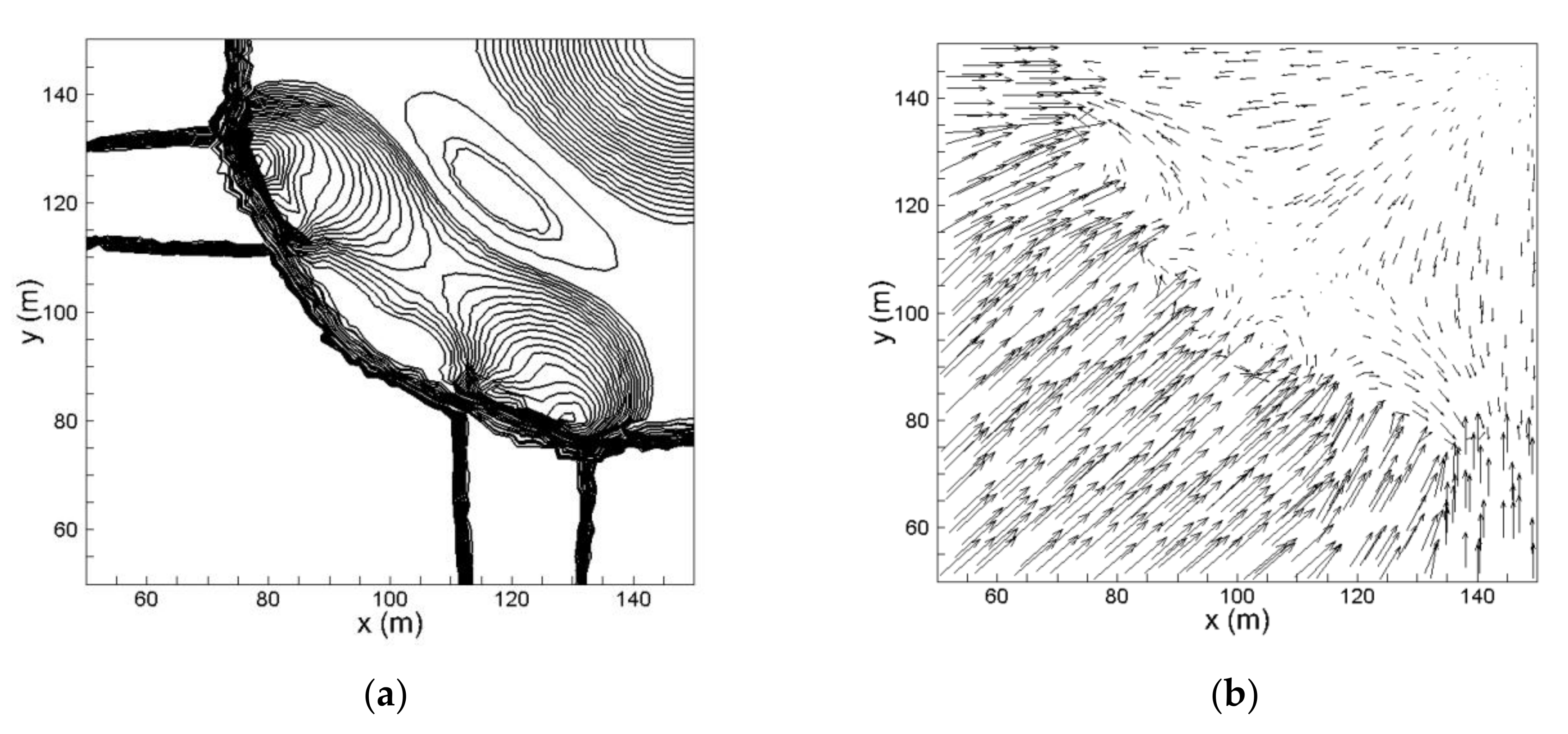
Figure 24 illustrates the contours of water surface elevation (equidistance = 0.1 m) and the vector field of flow velocities calculated by the new scheme. The contours of the simulated water surface (Figure 24a) and the vector field of flow velocities (Figure 24b) are symmetric about the bottom-left to top-right diagonal line of the domain. All the shock waves are perfectly captured, caused by the interactions between neighboring regions, indicating the excellent shock-capturing capability of the new scheme.
5. Conclusions
A new multislope MUSCL scheme on triangular grids is proposed in this paper within the framework of the Godunov-type CCFV method for simulating 2D shallow water flows over uneven topography. The values of flow variables on both sides of the considered edge are calculated by an edge-based reconstructing and limiting procedure where the upwind slope is easily obtained, since the upwind point is fixed at the node corresponding to the considered edge. Moreover, the downwind slope is also easy to evaluate by means of a straightforward criterion. The algorithm is simplified in the reconstructing and limiting procedures compared with the conventional LCD scheme [27] and other existing multislope MUSCL schemes [17,34], so computation cost is obviously reduced without sacrificing accuracy and robustness.
Seven tests were carried out to verify this scheme. The results show that lower time cost for reaching convergent results is achieved compared with the classical monoslope and multislope MUSCL schemes. In addition, it is also shown that this new scheme is more flexible on triangular grids and more straightforward to implement for taking account of the geometrical characteristics of triangular grids without sacrificing accuracy, robustness, and resolution. Furthermore, this new multislope reconstruction method is independent of HLLC approximated Riemann solvers and SWEs, so it can be integrated with numerical schemes based on other hyperbolic-type equations and Riemann solvers. To sum up, the new scheme provides an ideal alternative to the existing monoslope and multislope MUSCL schemes for numerically solving SWEs and other hyperbolic-type equations.
Author Contributions
Haiyong Xu designed and carried out the simulations and wrote the paper; Xingnian Liu contributed to the conception of the study; Fujian Li analyzed the data; Sheng Huang contributed materials and analysis tools; Chao Liu revised the manuscript.
Funding
This research was supported by the National Key Research and Development Plan (No. 2016YFC0402101) and National Natural Science Foundation of China (Nos. 51609160, 51539007).
Conflicts of Interest
The authors declare no conflict of interest.
References
- Thacker, W.C. Some exact solutions to the nonlinear shallow-water wave equations. J. Fluid Mech. 1981, 107, 499–508. [Google Scholar] [CrossRef]
- Zoppou, C.; Roberts, S. Explicit schemes for dam-break simulations. J. Hydraul. Eng. 2003, 129, 11–34. [Google Scholar] [CrossRef]
- Xing, Y.; Shu, C.-W. High order finite difference WENO schemes with the exact conservation property for the shallow water equations. J. Comput. Phys. 2005, 208, 206–227. [Google Scholar] [CrossRef]
- Liang, S.-J.; Tang, J.-H.; Wu, M.-S. Solution of shallow-water equations using least-squares finite-element method. Acta Mech. Sin. 2008, 24, 523–532. [Google Scholar] [CrossRef]
- Nikolos, I.K.; Delis, A.I. An unstructured node-centered finite volume scheme for shallow water flows with wet/dry fronts over complex topography. Comput. Methods Appl. Mech. Eng. 2009, 198, 3723–3750. [Google Scholar] [CrossRef]
- Nair, R.D.; Thomas, S.J.; Loft, R.D. A discontinuous Galerkin global shallow water model. Mon. Weather Rev. 2005, 133, 876–888. [Google Scholar] [CrossRef]
- Delis, A.I.; Nikolos, I.K.; Kazolea, M. Performance and comparison of cell-centered and node-centered unstructured finite volume discretizations for shallow water free surface flows. Arch. Comput. Methods Eng. 2011, 18, 57–118. [Google Scholar] [CrossRef]
- Godunov, S.K. A difference method for numerical calculation of discontinuous solutions of the equations of hydrodynamics. Mat. Sb. 1959, 89, 271–306. [Google Scholar]
- Rogers, B.D.; Borthwick, A.G.; Taylor, P.H. Mathematical balancing of flux gradient and source terms prior to using Roe’s approximate Riemann solver. J. Comput. Phys. 2003, 192, 422–451. [Google Scholar] [CrossRef]
- Hou, J.; Liang, Q.; Zhang, H.; Hinkelmann, R. An efficient unstructured MUSCL scheme for solving the 2D shallow water equations. Environ. Model. Softw. 2015, 66, 131–152. [Google Scholar] [CrossRef]
- Barth, T.; Jespersen, D. The design and application of upwind schemes on unstructured meshes. In Proceedings of the 27th Aerospace Sciences Meeting, Reno, NV, USA, 9–12 January 1989. [Google Scholar]
- Evangelista, S.; Greco, M.; Leopardi, A.; Vacca, A. A new algorithm for bank-failure mechanisms in 2D morphodynamic models with unstructured grids. Int. J. Sediment Res. 2015, 30, 382–391. [Google Scholar] [CrossRef]
- Evangelista, S.; Greco, M.; Leopardi, A. Numerical modeling of geomorphic processes in the presence of slope failures. In Proceedings of the 36th IAHR World Congress, Delft-Le Hague, The Netherlands, 28 June–3 July 2015. [Google Scholar]
- Audusse, E.; Bouchut, F.; Bristeau, M.-O.; Klein, R.; Perthame, B. A fast and stable well-balanced scheme with hydrostatic reconstruction for shallow water flows. SIAM J. Sci. Comput. 2004, 25, 2050–2065. [Google Scholar] [CrossRef]
- Audusse, E.; Bristeau, M.-O. A well-balanced positivity preserving “second-order” scheme for shallow water flows on unstructured meshes. J. Comput. Phys. 2005, 206, 311–333. [Google Scholar] [CrossRef]
- Bradford, S.F.; Sanders, B.F. Finite-volume model for shallow-water flooding of arbitrary topography. J. Hydraul. Eng. 2002, 128, 289–298. [Google Scholar] [CrossRef]
- Delis, A.I.; Nikolos, I.K. A novel multidimensional solution reconstruction and edge-based limiting procedure for unstructured cell-centered finite volumes with application to shallow water dynamics. Int. J. Numer. Meth. Fluids 2013, 71, 584–633. [Google Scholar] [CrossRef]
- Liang, Q. Flood simulation using a well-balanced shallow flow model. J. Hydraul. Eng. 2010, 136, 669–675. [Google Scholar] [CrossRef]
- Liang, Q.; Borthwick, A.G. Adaptive quadtree simulation of shallow flows with wet–dry fronts over complex topography. Comput. Fluids 2009, 38, 221–234. [Google Scholar] [CrossRef]
- Liang, Q.; Marche, F. Numerical resolution of well-balanced shallow water equations with complex source terms. Adv. Water Resour. 2009, 32, 873–884. [Google Scholar] [CrossRef]
- Van Leer, B. Towards the ultimate conservative difference scheme. V. A second-order sequel to Godunov’s method. J. Comput. Phys. 1979, 32, 101–136. [Google Scholar] [CrossRef]
- Buffard, T.; Clain, S. Monoslope and multislope MUSCL methods for unstructured meshes. J. Comput. Phys. 2010, 229, 3745–3776. [Google Scholar] [CrossRef] [Green Version]
- Kong, J.; Xin, P.; Shen, C.-J.; Song, Z.-Y.; Li, L. A high-resolution method for the depth-integrated solute transport equation based on an unstructured mesh. Environ. Model. Softw. 2013, 40, 109–127. [Google Scholar] [CrossRef]
- Zhang, D.; Jiang, C.; Cheng, L.; Liang, D. A refined r-factor algorithm for TVD schemes on arbitrary unstructured meshes. Int. J. Numer. Meth. Fluids 2016, 80, 105–139. [Google Scholar] [CrossRef] [Green Version]
- Van Leer, B. Towards the ultimate conservative difference scheme. IV. A new approach to numerical convection. J. Comput. Phys. 1977, 23, 276–299. [Google Scholar] [CrossRef]
- Van Albada, G.D.; Van Leer, B.; Roberts, W.W., Jr. A comparative study of computational methods in cosmic gas dynamics. Astron. Astrophys. 1982, 108, 76–84. [Google Scholar]
- Hubbard, M.E. Multidimensional slope limiters for MUSCL-type finite volume schemes on unstructured grids. J. Comput. Phys. 1999, 155, 54–74. [Google Scholar] [CrossRef]
- Davies, G. A well-balanced discretization for a shallow water inundation model. In Proceedings of the 19th International Congress on Modelling and Simulation (MODSIM), Perth, Australia, 12–16 December 2011; pp. 2824–2830. [Google Scholar]
- Toro, E.F.; Spruce, M.; Speares, W. Restoration of the contact surface in the HLL-Riemann solver. Shock Waves 1994, 4, 25–34. [Google Scholar] [CrossRef]
- George, D.L. Augmented Riemann solvers for the shallow water equations over variable topography with steady states and inundation. J. Comput. Phys. 2008, 227, 3089–3113. [Google Scholar] [CrossRef]
- Toro, E.F. Shock-Capturing Methods for Free-Surface Shallow Flows; Wiley: Chichester, UK, 2001. [Google Scholar]
- Harten, A.; Lax, P.D.; van Leer, B. On upstream differencing and Godunov-type schemes for hyperbolic conservation laws. SIAM Rev. 1983, 25, 35–61. [Google Scholar] [CrossRef]
- Hou, J.; Liang, Q.; Simons, F.; Hinkelmann, R. A 2D well-balanced shallow flow model for unstructured grids with novel slope source term treatment. Adv. Water Resour. 2013, 52, 107–131. [Google Scholar] [CrossRef]
- Le Touze, C.; Murrone, A.; Guillard, H. Multislope MUSCL method for general unstructured meshes. J. Comput. Phys. 2015, 284, 389–418. [Google Scholar] [CrossRef] [Green Version]
- Hou, J.; Liang, Q.; Zhang, H.; Hinkelmann, R. Multislope MUSCL method applied to solve shallow water equations. Comput. Math. Appl. 2014, 68, 2012–2027. [Google Scholar] [CrossRef]
- Barth, T.J.; Frederickson, P.O. Higher order solution of the Euler equations on unstructured grids using quadratic reconstruction. In Proceedings of the 28th AIAA Aerospace Sciences Meeting, Reno, NV, USA, 8–11 January 1990. [Google Scholar]
- Yoon, T.H.; Kang, S.-K. Finite volume model for two-dimensional shallow water flows on unstructured grids. J. Hydraul. Eng. 2004, 130, 678–688. [Google Scholar] [CrossRef]
- Park, J.S.; Yoon, S.-H.; Kim, C. Multi-dimensional limiting process for hyperbolic conservation laws on unstructured grids. J. Comput. Phys. 2010, 229, 788–812. [Google Scholar] [CrossRef]
- Venkatakrishnan, V. On the accuracy of limiters and convergence to steady state solutions. In Proceedings of the 31st Aerospace Sciences Meeting & Exhibit, Reno, NV, USA, 11–14 January 1993. [Google Scholar]
- Begnudelli, L.; Sanders, B.F. Unstructured grid finite-volume algorithm for shallow-water flow and scalar transport with wetting and drying. J. Hydraul. Eng. 2006, 132, 371–384. [Google Scholar] [CrossRef]
- Brufau, P.; García-Navarro, P.; Vázquez-Cendón, M.E. Zero mass error using unsteady wetting–drying conditions in shallow flows over dry irregular topography. Int. J. Numer. Meth. Fluids 2004, 45, 1047–1082. [Google Scholar] [CrossRef]
- Brufau, P.; Vázquez-Cendón, M.E.; García-Navarro, P. A numerical model for the flooding and drying of irregular domains. Int. J. Numer. Meth. Fluids 2002, 39, 247–275. [Google Scholar] [CrossRef]
- Kuiry, S.N.; Pramanik, K.; Sen, D. Finite volume model for shallow water equations with improved treatment of source terms. J. Hydraul. Eng. 2008, 134, 231–242. [Google Scholar] [CrossRef]
- Hou, J.; Simons, F.; Mahgoub, M.; Hinkelmann, R. A robust well-balanced model on unstructured grids for shallow water flows with wetting and drying over complex topography. Comput. Methods Appl. Mech. Eng. 2013, 257, 126–149. [Google Scholar] [CrossRef]
- Zhou, J.G.; Causon, D.M.; Mingham, C.G.; Ingram, D.M. The surface gradient method for the treatment of source terms in the shallow-water equations. J. Comput. Phys. 2001, 168, 1–25. [Google Scholar] [CrossRef]
- Ricchiuto, M.; Abgrall, R.; Deconinck, H. Application of conservative residual distribution schemes to the solution of the shallow water equations on unstructured meshes. J. Comput. Phys. 2007, 222, 287–331. [Google Scholar] [CrossRef]
- Gallardo, J.M.; Parés, C.; Castro, M. On a well-balanced high-order finite volume scheme for shallow water equations with topography and dry areas. J. Comput. Phys. 2007, 227, 574–601. [Google Scholar] [CrossRef]
- Marche, F.; Bonneton, P.; Fabrie, P.; Seguin, N. Evaluation of well-balanced bore-capturing schemes for 2D wetting and drying processes. Int. J. Numer. Meth. Fluids 2007, 53, 867–894. [Google Scholar] [CrossRef]
- Sampson, J.; Easton, A.; Singh, M. Moving boundary shallow water flow in circular paraboloidal basins. In Proceedings of the Sixth Engineering Mathematics and Applications Conference, 5th International Congress on Industrial and Applied Mathematics, Sydney, Australia, 7–11 July 2003. [Google Scholar]
- Aricò, C.; Sinagra, M.; Tucciarelli, T. Anisotropic potential of velocity fields in real fluids: Application to the MAST solution of shallow water equations. Adv. Water Resour. 2013, 62, 13–36. [Google Scholar] [CrossRef] [Green Version]
- Murillo, J.; García-Navarro, P.; Burguete, J.; Brufau, P. The influence of source terms on stability, accuracy and conservation in two-dimensional shallow flow simulation using triangular finite volumes. Int. J. Numer. Meth. Fluids 2007, 54, 543–590. [Google Scholar] [CrossRef]
- Duran, A. A robust and well-balanced scheme for the 2D Saint-Venant system on unstructured meshes with friction source term. Int. J. Numer. Meth. Fluids 2015, 78, 89–121. [Google Scholar] [CrossRef]
- Rajaratnam, N.; Ahmadi, R. Hydraulics of channels with flood-plains. J. Hydraul. Res. 1981, 19, 43–60. [Google Scholar] [CrossRef]
- Liu, C.; Luo, X.; Liu, X.; Yang, K. Modeling depth-averaged velocity and bed shear stress in compound channels with emergent and submerged vegetation. Adv. Water Resour. 2013, 60, 148–159. [Google Scholar] [CrossRef]
- Shan, Y.; Liu, X.; Yang, K.; Liu, C. Analytical model for stage-discharge estimation in meandering compound channels with submerged flexible vegetation. Adv. Water Resour. 2017, 108, 170–183. [Google Scholar] [CrossRef]
- Ye, J.; McCorquodale, J.A. Depth-averaged hydrodynamic model in curvilinear collocated grid. J. Hydraul. Eng. 1997, 123, 380–388. [Google Scholar] [CrossRef]
- Brio, M.; Zakharian, A.R.; Webb, G.M. Two-dimensional Riemann solver for Euler equations of gas dynamics. J. Comput. Phys. 2001, 167, 177–195. [Google Scholar] [CrossRef]
- Guinot, V. Godunov-Type Schemes: An Introduction for Engineers; Elsevier: Amsterdam, The Netherlands, 2003. [Google Scholar]
Figure 1.
Sketch of shallow water flow over uneven topography.

Figure 2.
Notations of a typical triangular cell and its three neighbors.

Figure 3.
Structure of the Harten–Lax–van Leer–contact (HLLC) approximated Riemann solver.

Figure 4.
Sketch of Touze’s scheme on triangular grids.

Figure 5.
Sketch of the new scheme on triangular grids: (a) case (a); (b) case (b).

Figure 6.
Comparisons between numerical and analytical results at t = 1500 s: (a) water surface; (b) unit width discharges in x and y directions.
Figure 6.
Comparisons between numerical and analytical results at t = 1500 s: (a) water surface; (b) unit width discharges in x and y directions.

Figure 7.
Global relative errors of unit width discharges in x and y directions.

Figure 8.
Computational mesh in the potential flow test.

Figure 9.
Numerical results of the potential flow test: (a) contours of water depth; (b) vector field of flow velocities.
Figure 9.
Numerical results of the potential flow test: (a) contours of water depth; (b) vector field of flow velocities.

Figure 10.
Sketch of water sloshing in a parabolic basin.

Figure 11.
Comparison between simulated and analytical water surface for the mesh of ∆L = 55.18 m. (a) t = T; (b) t = T + T/3; (c) t = T + T/2; (d) t = 2T + T/6.
Figure 11.
Comparison between simulated and analytical water surface for the mesh of ∆L = 55.18 m. (a) t = T; (b) t = T + T/3; (c) t = T + T/2; (d) t = 2T + T/6.

Figure 12.
Comparison between simulated and analytical velocities for the mesh of ∆L = 55.18 m at the point (−5000, −100): (a) u velocity; (b) v velocity.
Figure 12.
Comparison between simulated and analytical velocities for the mesh of ∆L = 55.18 m at the point (−5000, −100): (a) u velocity; (b) v velocity.

Figure 13.
Relative error of total water volume in the parabolic basin.

Figure 14.
Errors of the numerical scheme in and norms at t = 3T for , and : (a) errors; (b) errors.
Figure 14.
Errors of the numerical scheme in and norms at t = 3T for , and : (a) errors; (b) errors.

Figure 15.
Four triangular mesh types used for computation: (a) Delaunay; (b) orthogonal-I; (c) orthogonal-II; (d) distorted.
Figure 15.
Four triangular mesh types used for computation: (a) Delaunay; (b) orthogonal-I; (c) orthogonal-II; (d) distorted.

Figure 16.
Global relative errors of water depth on different types of mesh.

Figure 17.
Comparisons between simulated and analytical water surface on the distorted mesh along: (a) the diagonal section; (b) the horizontal-symmetry section.
Figure 17.
Comparisons between simulated and analytical water surface on the distorted mesh along: (a) the diagonal section; (b) the horizontal-symmetry section.

Figure 18.
Sketch of a cross-section in a simplified compound channel.

Figure 19.
Comparison of experimental and simulated longitudinal velocities.

Figure 20.
Sketch of the Parshall flume: (a) section view of L-L; (b) plan view.

Figure 21.
Comparison of experimental and simulated results along the flume: (a) water surface; (b) x-directional velocity.
Figure 21.
Comparison of experimental and simulated results along the flume: (a) water surface; (b) x-directional velocity.

Figure 22.
Sketch of the symmetric 2D Riemann problem.

Figure 23.
Simulated water surface of the 2D Riemann problem in 3D view at t = 4 s.

Figure 24.
Numerical results of the 2D Riemann problem at t = 4 s: (a) contours of water surface elevation; (b) vector field of flow velocities.
Figure 24.
Numerical results of the 2D Riemann problem at t = 4 s: (a) contours of water surface elevation; (b) vector field of flow velocities.


Table 1.
Data of the physical experiment.
| D (cm) | d (cm) | h (cm) | B (cm) | b (cm) | Q (m3/s) | Sw × 103 | Fr |
|---|---|---|---|---|---|---|---|
| 11.28 | 1.52 | 9.75 | 71.1 | 50.8 | 0.027 | 0.45 | 0.37 |
Table 2.
Values of parameters of the experiment.
| A (m) | B (m) | C (m) | D (m) | E (m) | F (m) | G (m) | M (m) | N (m) | T (m) | W (m) |
|---|---|---|---|---|---|---|---|---|---|---|
| 0.389 | 0.381 | 0.305 | 0.305 | 0.267 | 0.152 | 0.483 | 2.54 | 0.086 | 0.889 | 0.152 |
Table 3.
Initial conditions for the 2D Riemann problem.
| Region (#) | Coordinates (m) | Water Depth (m) | u (m/s) | v (m/s) |
|---|---|---|---|---|
| 1 | x ≤ 100, y ≤ 100 | 1 | 10 | 10 |
| 2 | x > 100, y ≤ 100 | 1 | 0 | 10 |
| 3 | x ≤ 100, y > 100 | 1 | 10 | 0 |
| 4 | x > 100, y > 100 | 10 | 0 | 0 |
© 2018 by the authors. Licensee MDPI, Basel, Switzerland. This article is an open access article distributed under the terms and conditions of the Creative Commons Attribution (CC BY) license (http://creativecommons.org/licenses/by/4.0/).
Share and Cite
MDPI and ACS Style
Xu, H.; Liu, X.; Li, F.; Huang, S.; Liu, C. A Novel Multislope MUSCL Scheme for Solving 2D Shallow Water Equations on Unstructured Grids. Water 2018, 10, 524. https://doi.org/10.3390/w10040524
AMA Style
Xu H, Liu X, Li F, Huang S, Liu C. A Novel Multislope MUSCL Scheme for Solving 2D Shallow Water Equations on Unstructured Grids. Water. 2018; 10(4):524. https://doi.org/10.3390/w10040524
Chicago/Turabian StyleXu, Haiyong, Xingnian Liu, Fujian Li, Sheng Huang, and Chao Liu. 2018. "A Novel Multislope MUSCL Scheme for Solving 2D Shallow Water Equations on Unstructured Grids" Water 10, no. 4: 524. https://doi.org/10.3390/w10040524
Note that from the first issue of 2016, this journal uses article numbers instead of page numbers. See further details here.