Some Aspects of Turbulent Mixing of Jets in the Marine Environment


1
Department of Civil, Environmental, Land, Building Engineering & Chemistry, Polytechnic University of Bari, Via E. Orabona 4, 70125 Bari, Italy
2
Department of Civil Engineering, University of Dundee, Dundee DD14HN, UK
*
Author to whom correspondence should be addressed.
Water 2018, 10(4), 522; https://doi.org/10.3390/w10040522
Submission received: 6 March 2018
/
Revised: 8 April 2018
/
Accepted: 13 April 2018
/
Published: 21 April 2018
(This article belongs to the Special Issue Turbulence in River and Maritime Hydraulics)
Abstract
:Prominent among environmental problems is the pollution of the coastal marine zone as a result of anthropogenic activities. On this point, while studies of jets in still water and in crossflows have been developed in many research centres, studies on jets interacting with waves are still rare. The present study analyses turbulent, non-buoyant water jets issued into a wave environment. A comparison of the time-averaged and phase-averaged velocity components has been carried out, in order to highlight the flow patterns in the two configurations. The experimental data have also been compared with others in the literature, such as the relationship between the dimensionless, longitudinal, time-averaged velocities of the jet mean axis and the distance from the source. Such comparisons reveal a good agreement. Furthermore, using the analogy between the equation of the turbulent transport of a solute concentration and the equation of the turbulent kinetic energy, the paper presents also estimates of the turbulence diffusion coefficients and advection terms of jets in a wave environment. The experimental results are compared with jets in still water. With the presence of waves, the turbulence length-scales in the streamwise direction vary, contributing to an increase in streamwise turbulent diffusion, relative to the condition of the same jet in still water. The analysis of the jet streamwise advection term reveals that it increases in the case of jets in a wave environment, as compared to no-wave conditions.
1. Introduction
The explosive global economic growth initiated in the 1960s has surely left its mark on hydraulic engineering and on a wide spectrum of environmental problems. Prominent among these problems is the pollution of the coastal marine environment as a result of anthropogenic activities associated with, for example, (i) the discharge of domestic and industrial wastewater; (ii) the unregulated and accidental release of petroleum and hydrocarbon products from marine traffic and offshore exploration/production installations; (iii) the run-off of animal waste and fertiliser-derived nutrients from agricultural land; and (iv) the construction of marine structures and waste disposal and treatment systems. All these consequences have an impact on population health, marine ecology, economic prosperity, commercial operations, and environmental sustainability. The impact is felt throughout the spheres of water management (drinking water, industrial water, bathing water, irrigation, hydropower, etc.), navigation (currents, ice formation, shoaling, erosion involving dredging, protection works, etc.), flood protection (forecasting, dike placement, regulation of discharges), traffic management (tunnels, bridges, harbours, etc.), near- and offshore activities (modifications to coastal currents and eddies, ice drifts, blow-outs, etc.), and commercial and leisure fishing (modifications to currents, salinity, temperature, oxygen content; formation of fronts, etc.). The prediction and management of pollution problems is surely becoming more and more pressing, with massive consequences for the environmental and ecological health of coastal waters and their surrounding communities [1,2,3,4,5].
In the present article, focus is placed upon the importance of turbulent mixing and entrainment processes for typical near-shore and estuarial conditions where the effective and safe disposal of wastewater is the principal objective. Attention is directed towards the role of turbulent jets [6,7,8] in accomplishing this mixing. In the marine environment, such jets are almost always associated with wastewater outfalls that have been constructed to convey treated wastewater from onshore treatment plants to zones appropriately far from shore (i) to prevent contamination of the waters in the near-shore region and (ii) to minimise the harmful effects of the discharge on humans and indigenous flora and fauna. The monographs by Wood et al. [9] and Roberts et al. [10] and the chapter by Tate et al. [11] provide comprehensive entry points to the extensive relevant literature on this topic. Finally, it is noted that, though the emphasis here is on the behaviour and properties of the turbulent buoyant jets, the dilution (and eventual fate) of contaminants discharged within the effluents is controlled also by the spatio-temporal structure of the ambient turbulence field in the receiving waters. In most cases, this structure is determined by the receiving water bathymetry and topography and the strength and variability of wind, tides, heat exchange, evaporation, ice formation, barometric pressure variation, gravity, etc. The spatio-temporal structure of the ambient turbulence field and the modifying role of (i) density stratification and (ii) vertical variations in mean flow is crucially important for the prediction of entrainment and mixing of turbulent jets discharged from wastewater outfalls. It is an area of research that requires further investigation.
The sea has always been the final destination for water-borne waste products coming from the land. In recent years, effects such as jet momentum, buoyancy, current, stratification, etc., on the processes of mixing and transport have received more and more attention [12,13,14,15,16], but wave action also plays a very important role in many cases [17,18,19]. While there are several studies in the literature on jets and their interaction with currents [9,20,21], few deal with jet–wave interaction, with the majority emphasizing the importance of a wave flow field in diffusion processes [22,23,24,25,26,27,28,29,30,31,32,33] and the necessity of experimental tests to explain jet–wave interaction dynamics and possibly confirm the validity of mathematical models present in literature [34]. The topic is of great engineering interest for environmental problems [9,35,36,37,38,39].
Shuto and Ti [17] carried out experiments to investigate the dilution rate of plumes with waves at the free surface. The authors found that the dilution rate is inversely proportional to the square of the ratio of the water depth to the outlet diameter and is proportional to the ratio of the discharge velocity to a characteristic horizontal velocity of the ambient fluid. Sharp [19] pointed out that longitudinal velocity component profiles of jets with waves show twin peaks in some jet cross sections (so-called “dumb-bell effect”, typical of sewage discharged into a tidal estuary). Chyan and Hwung [27] carried out experimental studies using a combined LDA (Laser Doppler Anemometry) and LIF (Laser-Induced Fluorescence) system to obtain a combined analysis of velocity components and concentration of nonbuoyant jets vertically discharged in a wave environment. Using flow visualisation, they identified three regions of a jet–wave interaction: (1) deflection region, (2) transition region, and (3) developed jet region. Chyan and Hwung [27] noted that the process of periodic jet deflection allows a large volume of water from the external environment to pour into this jet. The mechanism, which was called the “wave tractive mechanism”, adds to that of classic entrainment, thereby improving the dilution process. Koole and Swan [28] analysed 2D non-buoyant jet dispersion in a flow field of regular waves. They presented velocity profiles, standard deviation of the turbulent velocity components, and Reynolds shear stresses.
The studies cited above illustrate that some investigations have been undertaken on the interaction between jets and waves in the past, but there is still a need for further detailed analysis of this problem, utilizing data collected with modern instrumentation. This is a main motivation for the present study and the main novel component.
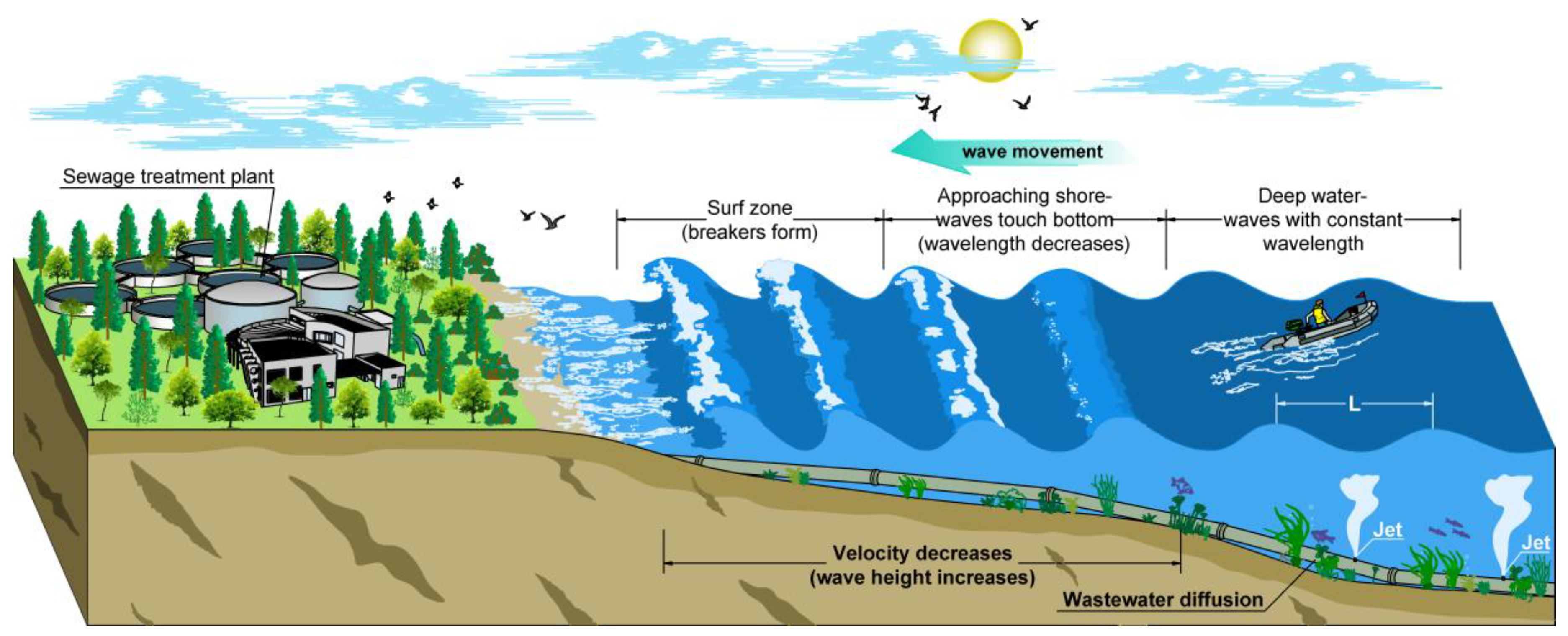
The principal purpose of this article is to highlight aspects of turbulent mixing in the marine environment (particularly for jet flows) in order (i) to raise awareness of the range of problems that still remain to be addressed and solved and (ii) to indicate future developments, directions, and perspectives in this field. The oft-cited dictum “Dilution is the Solution to Pollution” summarises the overall design objectives underlying many marine wastewater disposal systems, illustrating why environmental flows characterised by dilution and mixing processes are of great interest for researchers and practitioners. In the present article, recent theoretical analyses and experimental results are presented for some case studies of jets in a wave environment (see Figure 1).
The material to be presented here shows that deeper knowledge of these complex environmental flows should be pursued for research, technical, and engineering interests. Because of the increasing stress placed on water resources throughout the world, a resurgence and reinvention of hydraulic engineering should be considered, in the sense that hydraulic research will be more and more a cooperation with other experts and that researchers must respond to the need to manage and protect natural resources. Considering all these aspects, the old motto with which this summary starts could be changed to “Dilution is (not always) the Solution to Pollution”.
2. Materials and Methods
2.1. Momentum Equations
The fundamental equations governing the problem can be derived from the Navier–Stokes equations. Any physical quantity is split into the steady mean flow component, the fluctuation component due to the statistical contribution of the wave, and the fluctuation component of the turbulence [40]. Therefore, the ui (i = 1,2,3) velocity components can be expressed as follows:
where the angular brackets “< >” denote an operator representing an ensemble average, the tilde symbol indicates the fluctuations due to the wave statistical contribution (or oscillating components), the prime symbol indicates the turbulent fluctuations, and the capital letters or the over-bar indicate the steady mean flow (time-averaged components). In addition, t is time and the xi are the coordinates of a Cartesian frame.
Using the Cartesian tensor notation, the ensemble average of the motion equations for turbulent nonbuoyant jet flow under wave action is
where ρ is the water density, δij is the Kronecker delta, p is the hydrodynamic pressure, and μ is the dynamic viscosity. The motion of the incompressible fluid is periodic, so the average over the period T of Equation (2) becomes
2.2. Transport of Tracers and Turbulent Kinetic Energy
The time-averaged, turbulent transport of a solute concentration is described by the following equation:
where c(x1, x2, x3) is the solute concentration and Kii are the coefficients for dispersion. For further details see Mossa et al. [32,33].
In the analysis of the flow–dispersion interaction, the turbulent kinetic energy is important in determining the turbulent dispersion coefficient and, thus, the mass transport. For high Reynolds numbers, assuming that the production term is of order of the dissipation term, the equation of the turbulent kinetic energy is
where
is the time-averaged turbulent kinetic energy, which, in the case of 2D velocity measurements, can be estimated as proposed by Svendsen [41] with the following equation
The parameter Dk is the turbulent diffusion coefficient, which can be expressed as the product of a length scale and a velocity scale. A physical meaningful velocity scale is . Consequently, we consider
with l the integral length scale associated with turbulent eddies. Equation (5) is formally analogous to Equation (4) and, therefore, assuming that the Prandtl number is O(1), the cross-correlation between the time-averaged turbulent kinetic energy and the U, V, and W velocity components could be analysed and related to the time-averaged solute concentration C transport by the mean flow UC, VC, and WC.
Furthermore, analogously to Equation (6), Tanino and Nepf [42] assumed that the net dispersion coefficients of Equation (1) could be set equal to
where the scale factor α could be different for horizontal and vertical diffusion, even if generally it is of O(1). In the present study, the integral length scale li is evaluated by multiplying the integral time scale Tu by the local time-averaged velocity ui, where Tu is estimated by the autocorrelation function of the turbulent velocity fluctuations.
2.3. Experimental Procedure
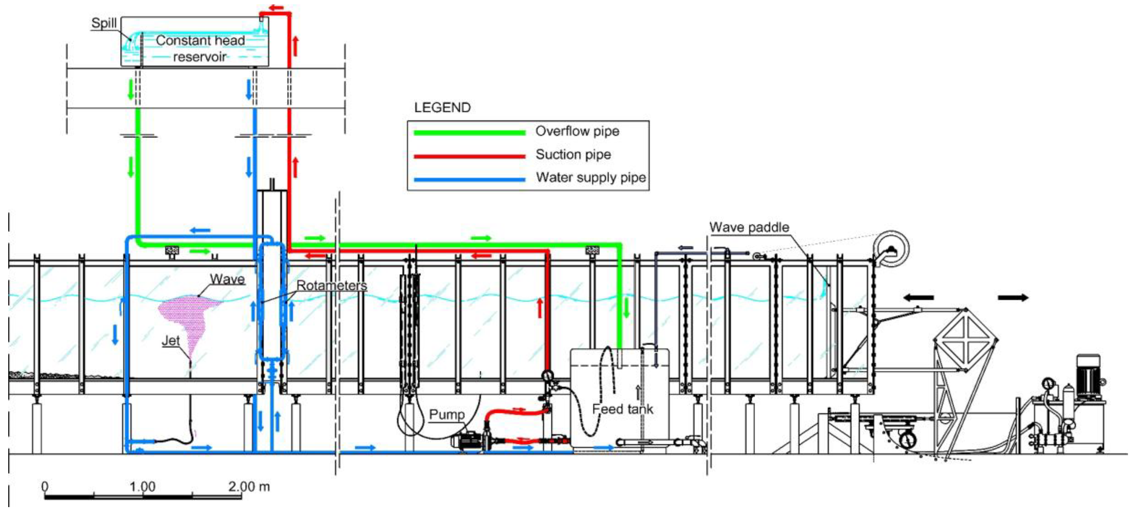
Experiments were carried out in a wave channel at the hydraulics laboratory of the Polytechnic University of Bari (Bari, Italy). The channel is about 45 m long and 1 m wide with walls made up of crystal plane sheets 1.2 m high, supported by iron frames with a centre-to-centre distance of about 0.44 m, where resistance probes for wave profile measurements may be placed. Figure 2 and Figure 3 show drawings of the laboratory system and the jet characteristics, respectively.
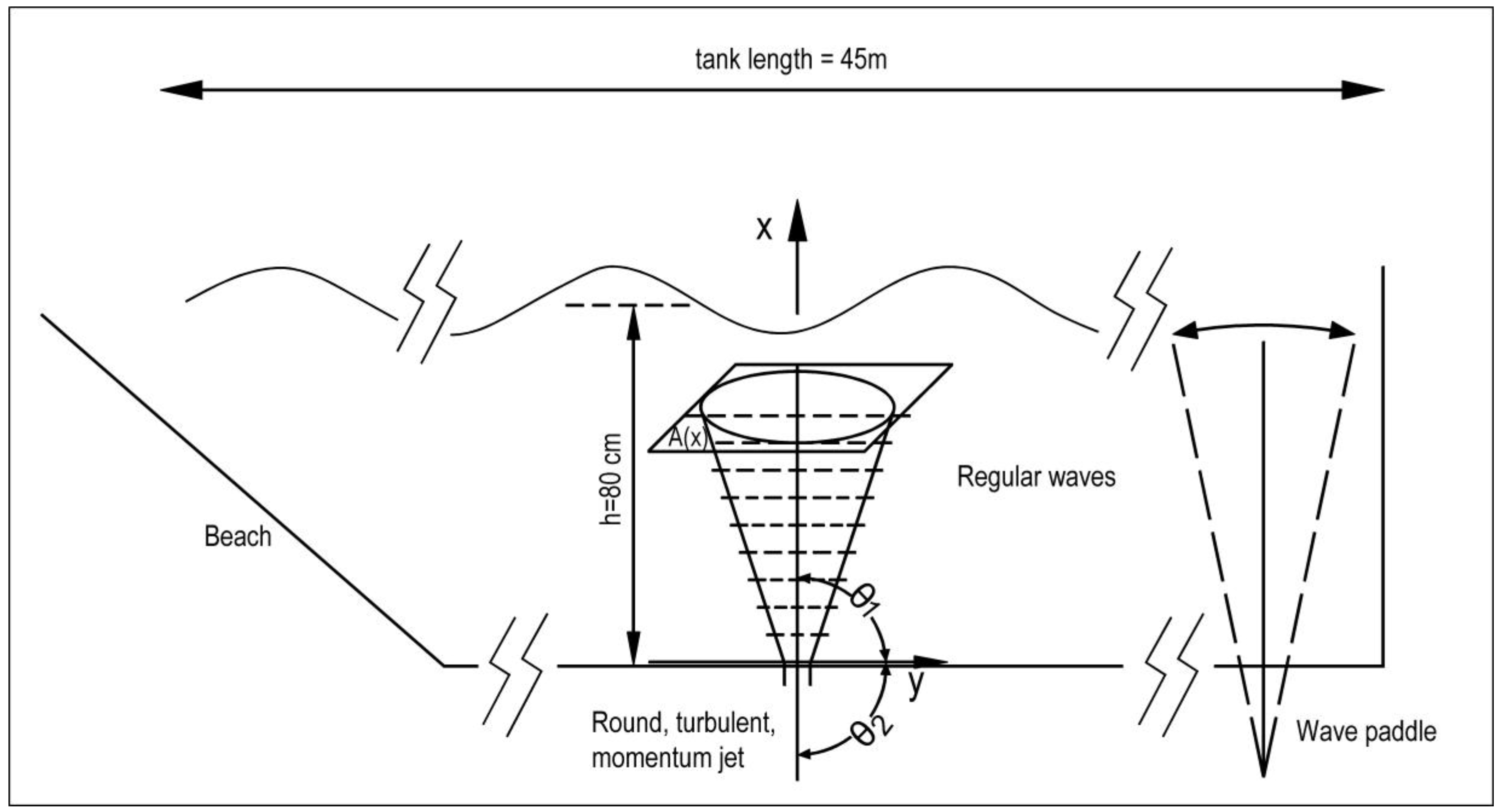
This study was carried out for a vertical turbulent nonbuoyant jet discharged in a stagnant environment and for the same jet interacting with progressive wave flow fields, in the intermediate range between deep and shallow water. During testing, the mean water depth near the paddle was h = 0.8 m.
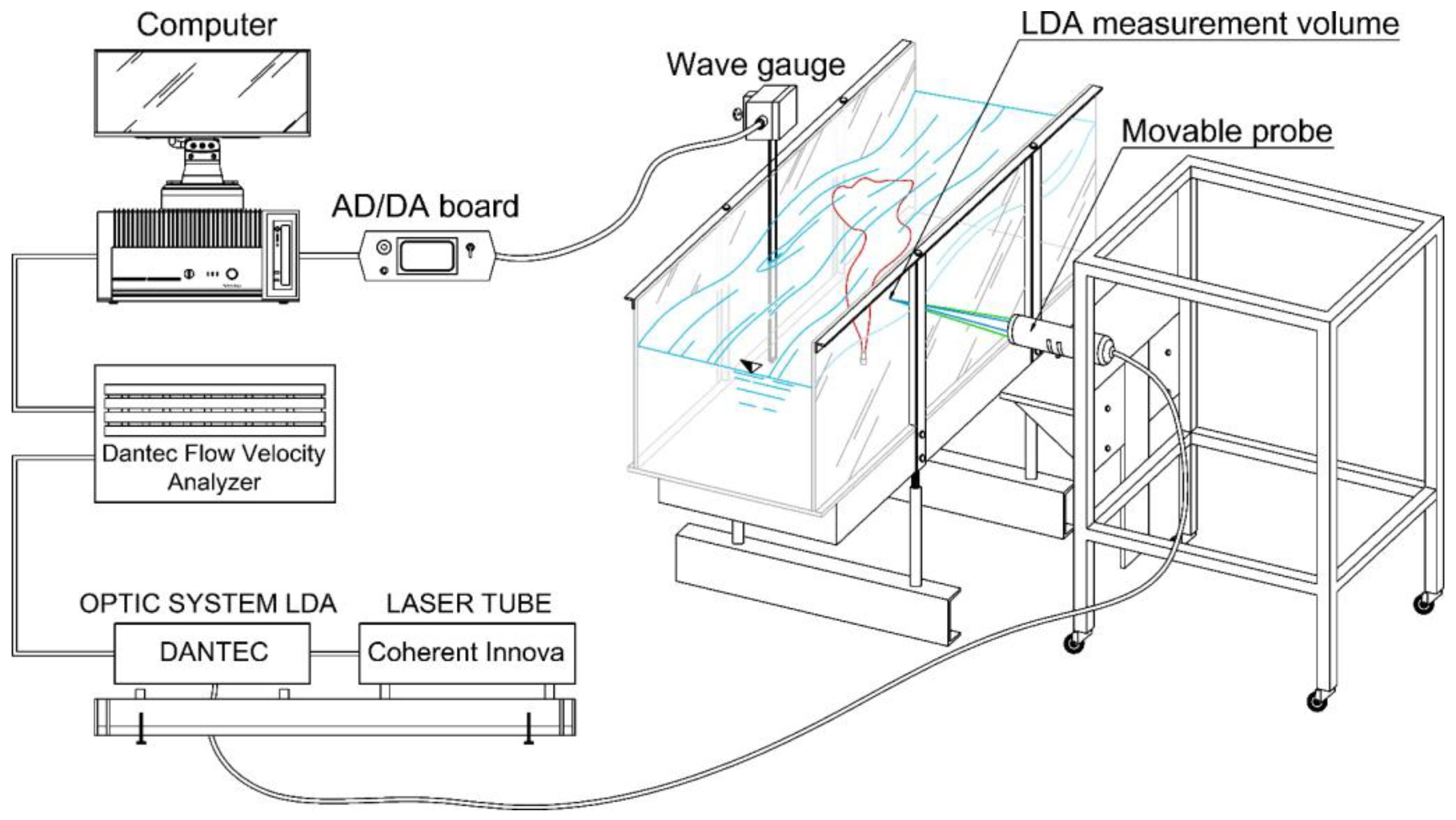
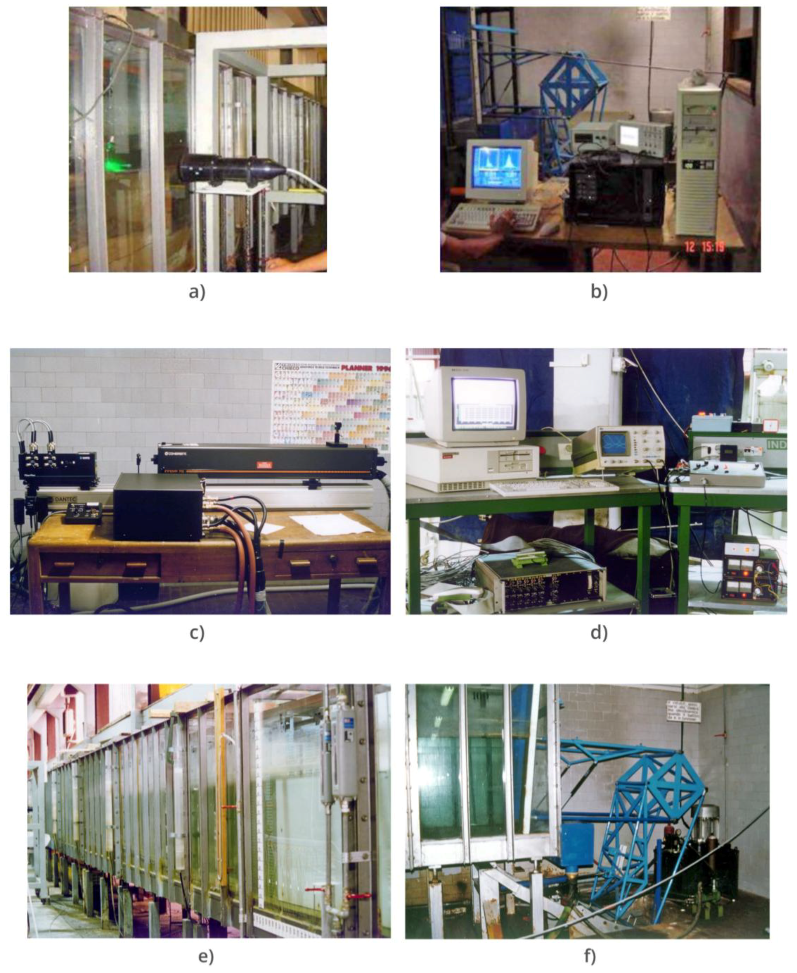
The velocity field was measured by using a backscatter, two-component four-beam fibre-optic LDA system (by Dantec Dynamics A/S, Skovlunde, Denmark). Particularly, the LDA system consists of a 5 W water-cooled argon-ion laser (version Innova 70, by Coherent Inc., Santa Clara, CA, USA), a 2D fibre flow transmitter (by Dantec Dynamics A/S, Skovlunde, Denmark, which comprises a transmitter providing colour separation and frequency shifting of the laser beam; fibre manipulators for optimum coupling of the laser light into optical fibres; a probe head with a fibre-optical connection to the transmitter; and back-scatter receiving optics including colour filters, colour separation, and photodetectors), a probe with a diameter of 85 mm (by Dantec Dynamics A/S, Skovlunde, Denmark, with a focal length of 310 mm and a beam spacing of 60 mm), and a signal processor (version 58N40 FVA-Flow Velocity Analyzer enhanced, by Dantec Dynamics A/S, Skovlunde, Denmark). The accuracy of velocity measurements is ±2%. Through an AD/DA-Analog to Digital/Digital to Analog board (Keithley Metrabyte model DAS 50/4), the laser Doppler data can be correlated with up to four 12-bit channels of auxiliary inputs coming from four transducers. Therefore, for the configurations of jets with waves, the measurement system allows us to assess—at the same time as the velocity components—the wave elevation profile, by use of a resistance wave gauge placed in the transversal section of the channel crossing the laser measurement volume. The entire system is assisted by a process computer (Figure 4).
Figure 5a–f show the different parts of the complex experimental apparatus, which comprises the LDA system, the resistance wave gauge system, and the wavemaker system.
The vertical nonbuoyant jet under consideration was introduced through a 2.01 mm inside-diameter circular nozzle, with a volume flow Q0 rate equal to 22.22 cm3/s; a discharge velocity U0 equal to 6.42 m/s; a momentum flux M = Q0U0 at the nozzle equal to 1.43 × 10⁻⁴ m4/s2; and Reynolds number, based on the nozzle diameter, equal to 13,482. The discharge scale length LQ = Q0/M0.5, which measures the distance over which the port geometry influences the jet behaviour, is equal to 1.9 mm (comparable with the nozzle diameter). The round nozzle was located about 11 m from the wavemaker at 16.7 cm from the bottom of the channel. The velocity components measured in the present study are u in the x direction (see Figure 3; velocity component parallel to the jet axis x, i.e., vertical velocity component, conventionally established as positive if oriented upward) and v in the horizontal direction (conventionally established as positive if oriented onshore).
Two categories of flow were considered; firstly, jet discharged into still water (i.e., configuration without waves) and, secondly, jet discharged into regular wave trains, generated in the channel, with a wave period for each configuration of 2.00 s (Test 1), 1.43 s (Test 2), and 1.00 s (Test 3), respectively. For the tests with waves, Table 1 (movies in supplementary) shows the wave height (H), the wave length (L), the wave period (T), the wave steepness H/L, the relative depth h/L, and Lw = M1/2/. The latter term is the length scale of the region from the nozzle dominated by the initial jet momentum compared to the wave-induced momentum, where , the values of which are also shown in the table, is a crossflow velocity scale of the wave motion, defined as [27]
with σ = 2π/T the wave angular frequency and k = 2π/L the wave number. The values of the relative depths h/L show that the jets of Table 1 are discharged in a wave transitional zone, i.e., between shallow and deep waters.
The wave flow field in the channel can be described with the Stokes second-order theory according to the classic Le Méhauté abacus [43]. The reflection coefficient in the channel is not greater than 9%.
In the cases of jets interacting with waves, ensemble-averaged velocities were obtained by phase-averaging the measured signals separated by the wave period. The results, which represented the phase-averaged velocities at different phases of a wave cycle, were averaged to yield the time-averaged velocities. The turbulent velocity fluctuations were obtained by subtracting the phase-averaged velocities from the original time series. For further details, see [32,33].
3. Results and Discussion
3.1. Jet Flow Patterns, and Phase- and Time-Averaged Velocities
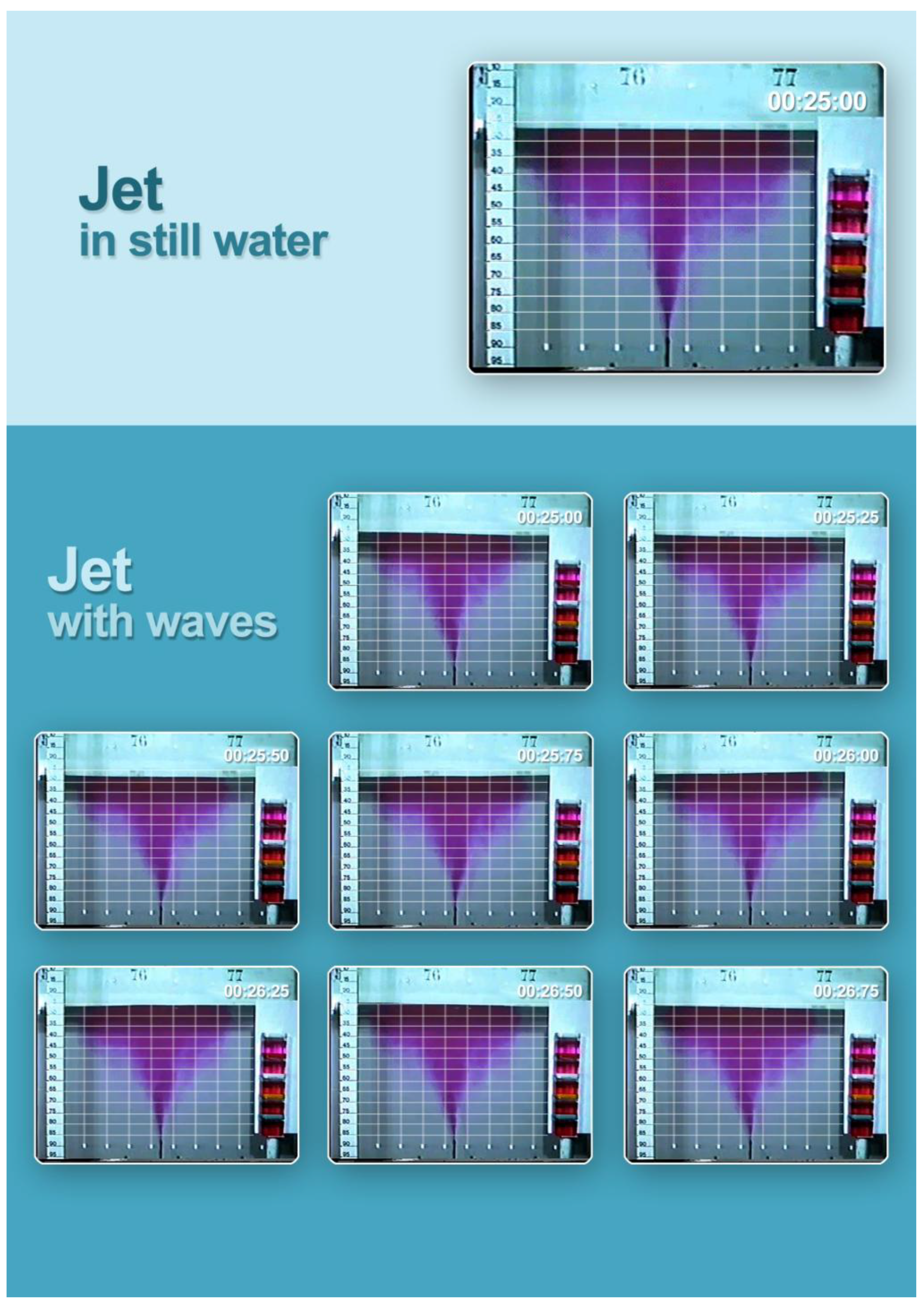
The jet flow in the unsteady and periodic wave flow field has the characteristics shown in Figure 6, which reports a sequence of pictures of the jet of Run 1 of Table 1 taken at one-eighth of the wave period, in comparison with the flow field of the same jet issued in still water.
The grid enables us to better show (i) the difference between the cases of jets with and without waves and (ii) the jet oscillations in the configurations where waves are present. Particularly, the jet issued into still water shows an enlargement that is described well in the literature [20,32,33]. Furthermore, in the case of the same jet with waves, the flow pattern resembles that of a jet discharged into a cross-current when the wave horizontal velocity dominates and that of a co-stream jet or jet in opposing flow when the vertical wave velocity dominates. As the wave motion changes periodically, different features will prevail by turns. The most impressive conclusion that we can obtain from these images is the enlargement of the jet area when waves are present compared with the turbulent jet in still water, which suggests an enhancement of the dilution and, therefore, a positive effect of the wave motion during the initial mixing processes.
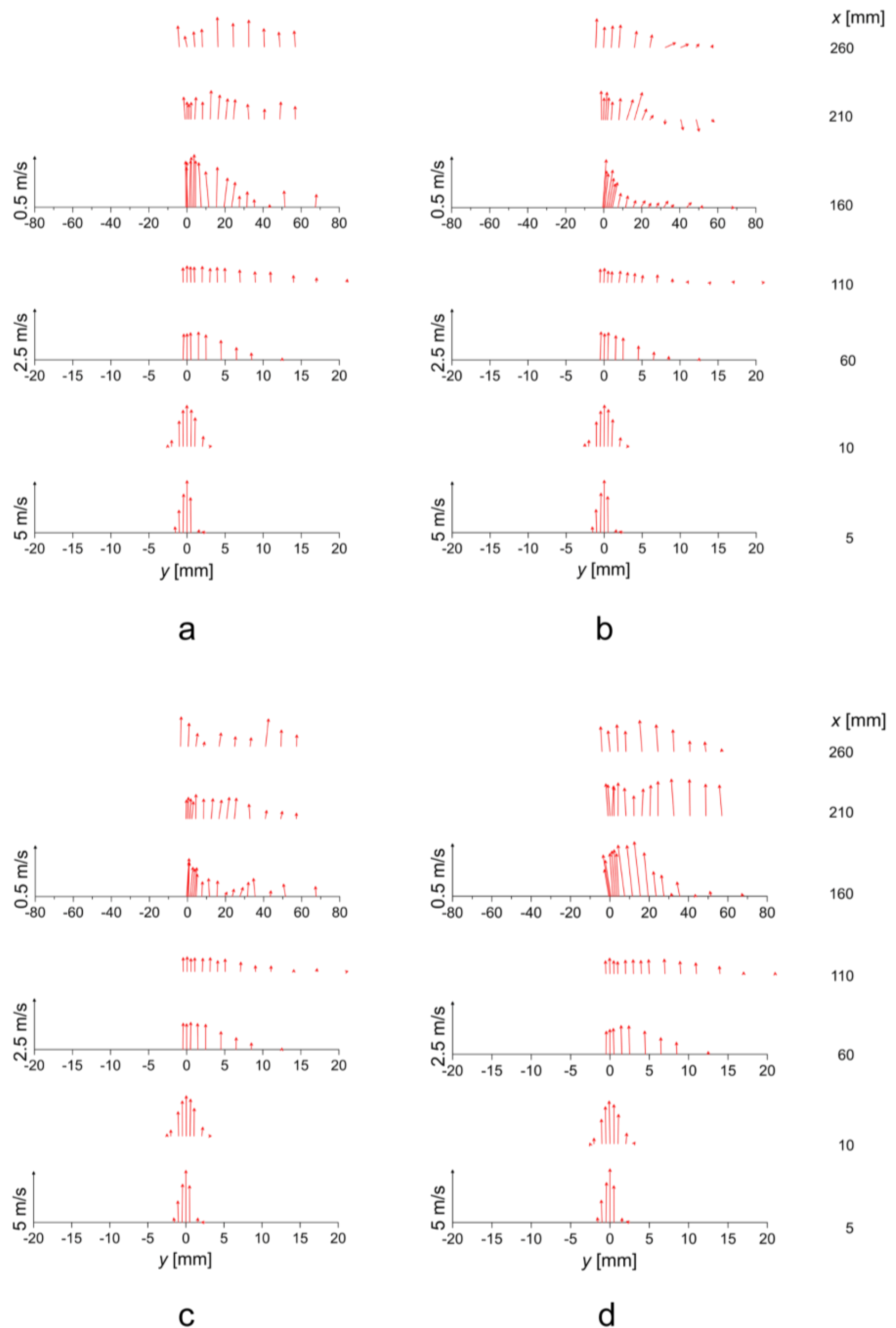
The flow patterns are confirmed with the results of the phase-averaged velocity vectors shown in Figure 7 for Run 1 of Table 1.
In this figure, it is possible to see the jet deflection back and forth by wave action, which agrees with the results of flow visualisation. The larger oscillations are present closer to the free surface, where the wave action is greater.
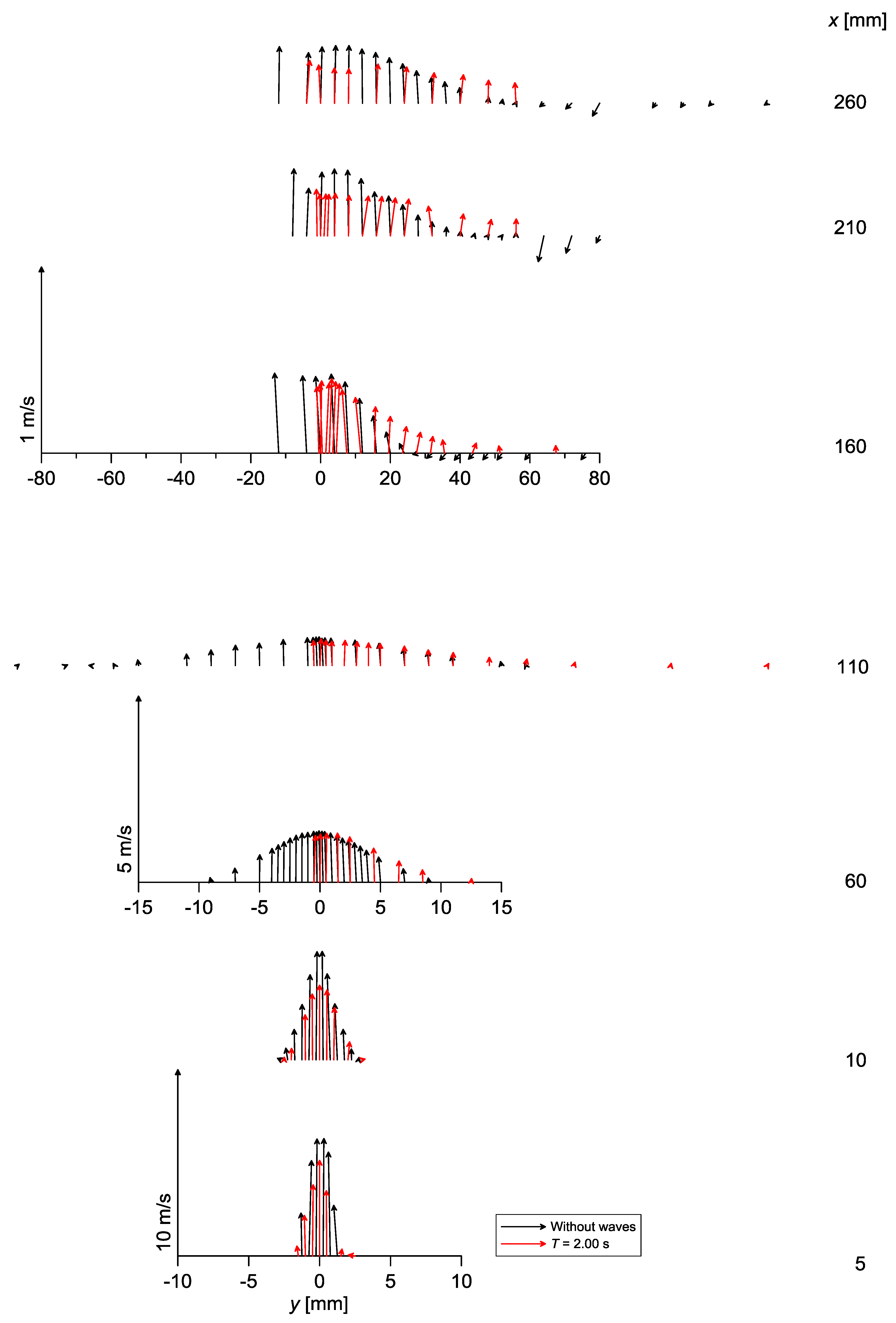
Figure 8 shows the time-averaged velocity vectors of Run 1 of Table 1 and of the same jet in still water.
The comparison enables us to highlight the differences between the two configurations. Particularly, the figure shows that the velocity profiles of jets discharged in a wave environment are even flatter and wider than those of the same jet discharged in a stagnant environment. These profiles clearly indicate the existence of a relapse flow, as observed also by [13]. In the region farther from the nozzle, vertical velocity profiles point out, at times clearly, the presence of two peaks. In the case of the jet with waves, it is possible to see also the presence of twin peaks, as a typical result of the jet deflection due to periodic wave motion [27,32,33].
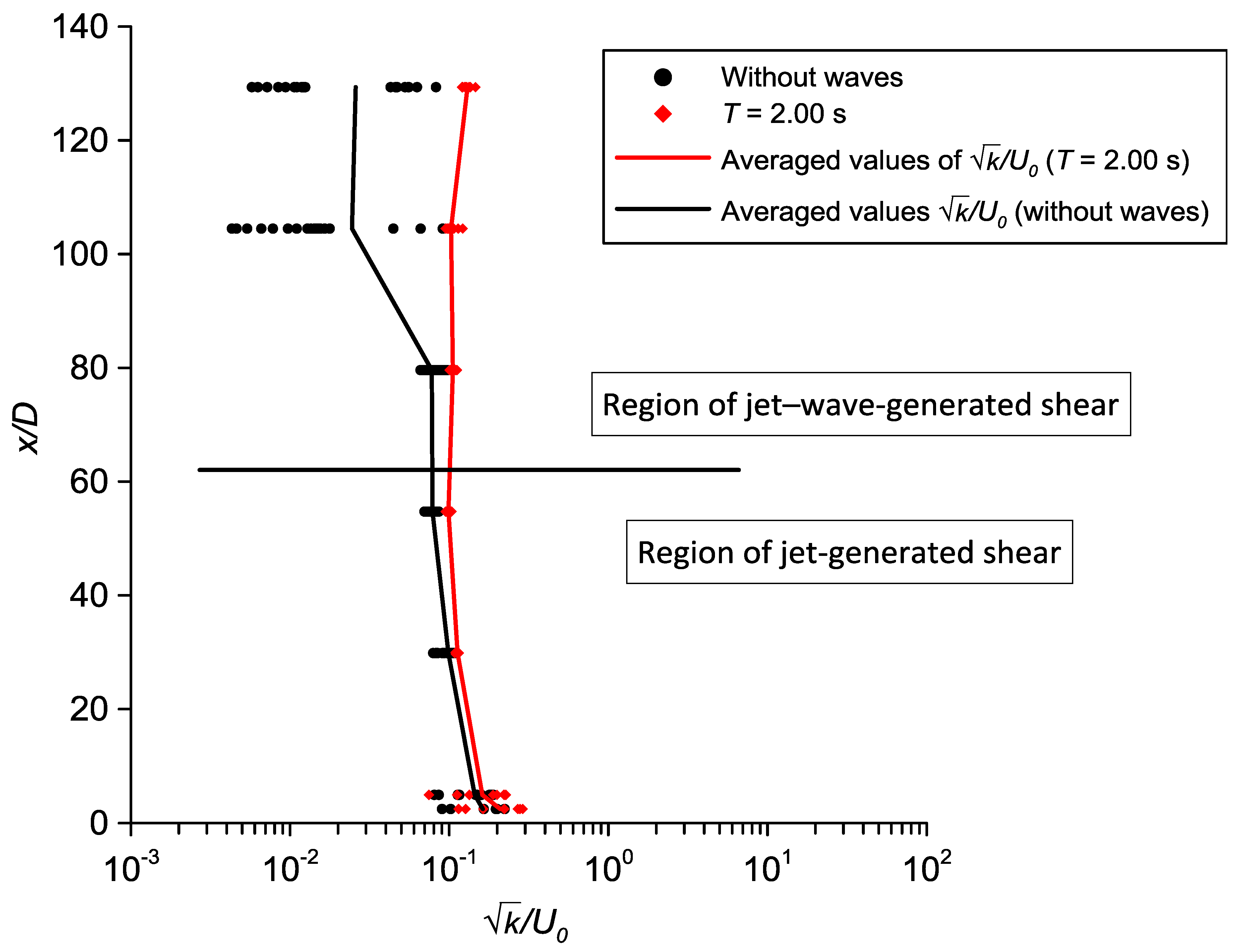
Figure 9 shows the values of the square root of the turbulent kinetic energy non-dimensionalised by U0 of Run 1 of Table 1. Close to the nozzle, specifically at x/D < 60 and x << Lw, the values of are similar with and without waves, indicating that the impact of the wave on the turbulent kinetic energy is small. This trend is also confirmed by the other runs. In this region it is possible to affirm that the turbulence is dominated by the jet and, therefore, this is the region with jet-generated shear. Farther from the nozzle, i.e., when x is closer to or greater than Lw, the values of are higher with the presence of waves. In this region the turbulence of the jet is also affected by the waves (region of jet–wave-generated shear).
Figure 9 shows also that, in the case of the absence of waves, the values of k reduce at a higher distance from the nozzle. On the contrary, in the case of the jet with waves, O(k) is almost constant in the upper region, demonstrating that the waves feed the jet turbulence.
3.2. Comparison with Previous Investigations
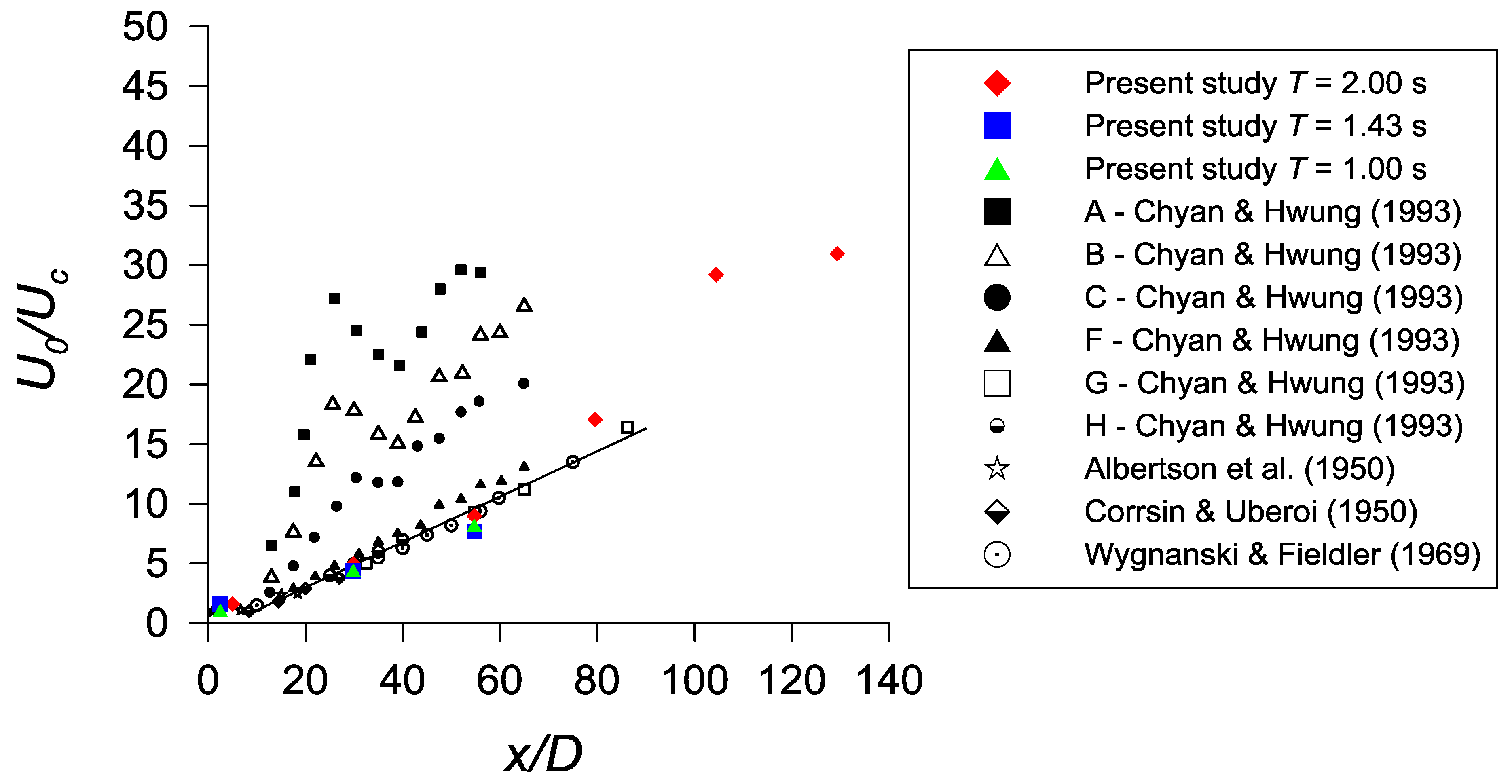
Figure 10 shows the values of the mean axial velocity Uc made dimensionless by the jet exit velocity U0. The results of the present study are compared with those of Albertson et al. [44], Corrsin and Uberoi [45], Wygnanski and Fieldler [46], and Chyan and Hwung [27]. In order to highlight the differences of the experimental conditions, Table 2 shows the main flow conditions and instrumentation used by the authors of the previous investigations.
It is important to consider that the classic relationships reported in Figure 10 can be applied in the fully developed flow region of a jet [20]. Furthermore, in the case of Run 1 of Table 1 of the present paper, where the measurements have also been assessed closer to the free surface where the wave action is more pronounced, Figure 10 shows that the last three points cannot be described by the classic laws, in agreement with Chyan and Hwung [27]. Therefore, using the experimental points of the jet’s fully developed region where the wave action is not more pronounced (i.e., until the section at 110 mm from the nozzle in the case of the present study), the absolute values of the relative errors between the experimental and theoretical values of U0/Uc have a mean value of 7.06% using the relationship by Albertson et al. [44], 6.29% using the relationship by Corrsin and Uberoi [45], and 6.72% using the relationship by Wygnanski and Fiedler [46]. It is possible to conclude that in this region the experimental results of the present paper are well fitted by the classic literature relationships.
3.3. Turbulent Diffusion Coefficients and Advection Terms
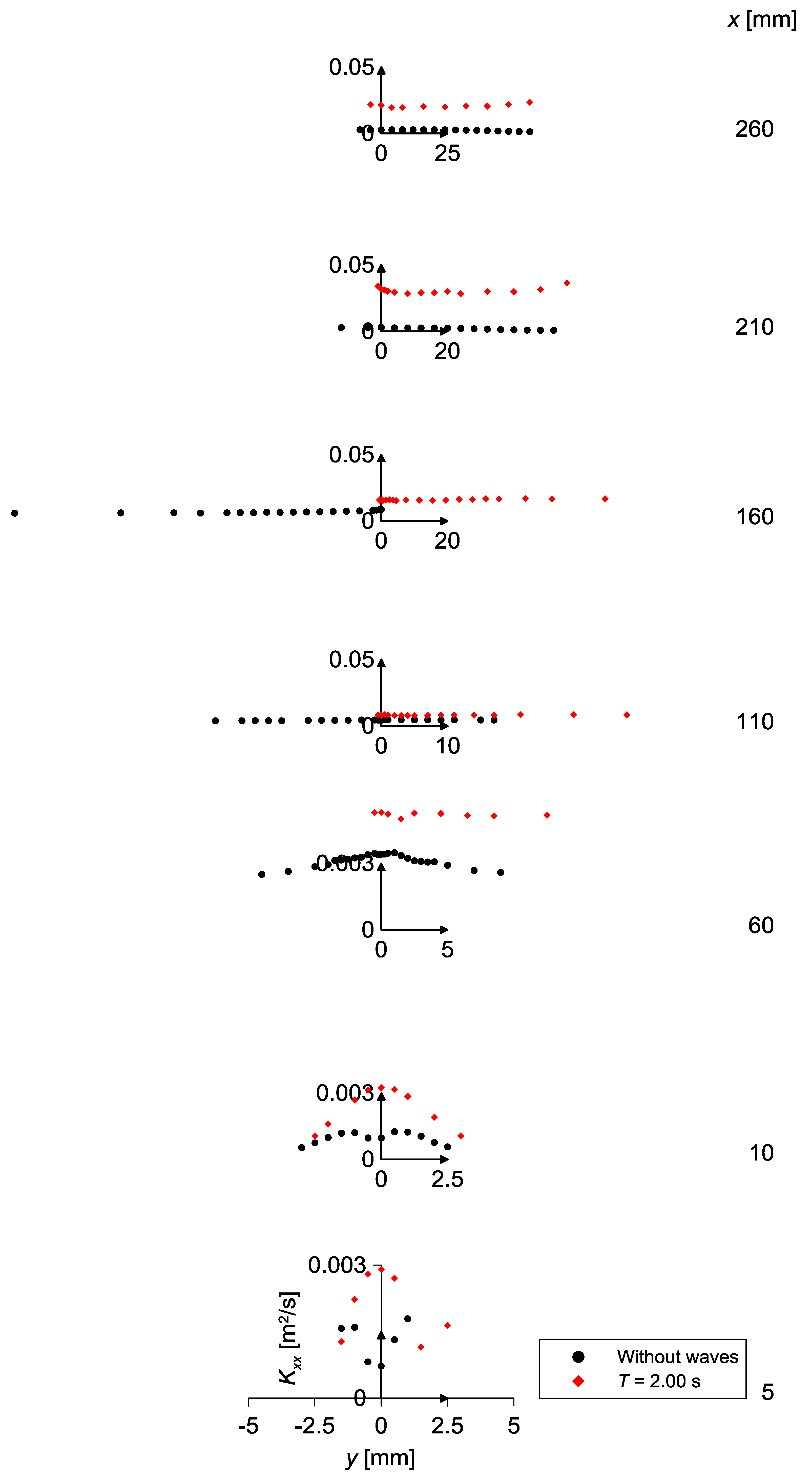
Figure 12 show the cross profile of the streamwise turbulent diffusion coefficient, Kxx, for Run 1 of Table 1 and for the same jet issued in still water estimated from Equation (9). It is possible to see that Kxx is greater in the case of the jet with waves.
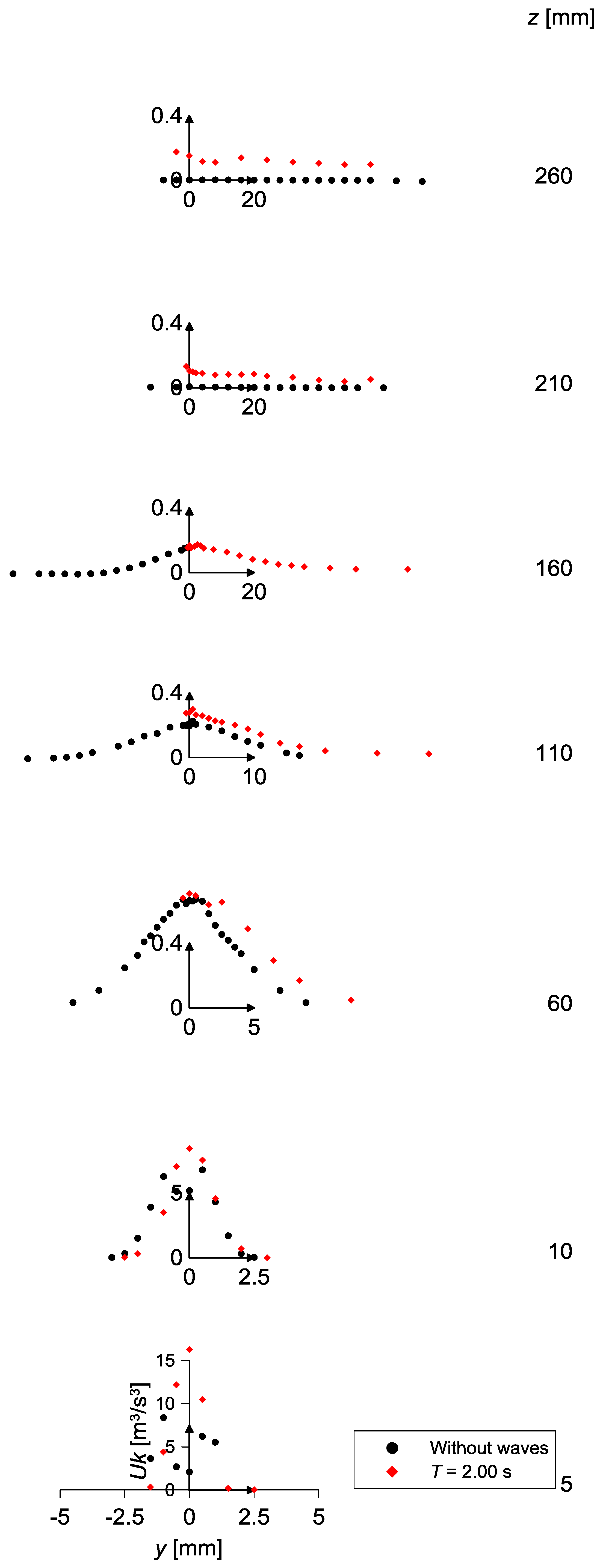
Figure 13 shows the vertical profiles of the advection term Uk of Run 1 of Table 1 and of the same jet issued in still water. The other configurations of jets with waves, not reported for the sake of brevity, confirm these results. It is possible to conclude that the longitudinal advection term is greater in the case of jets with waves.
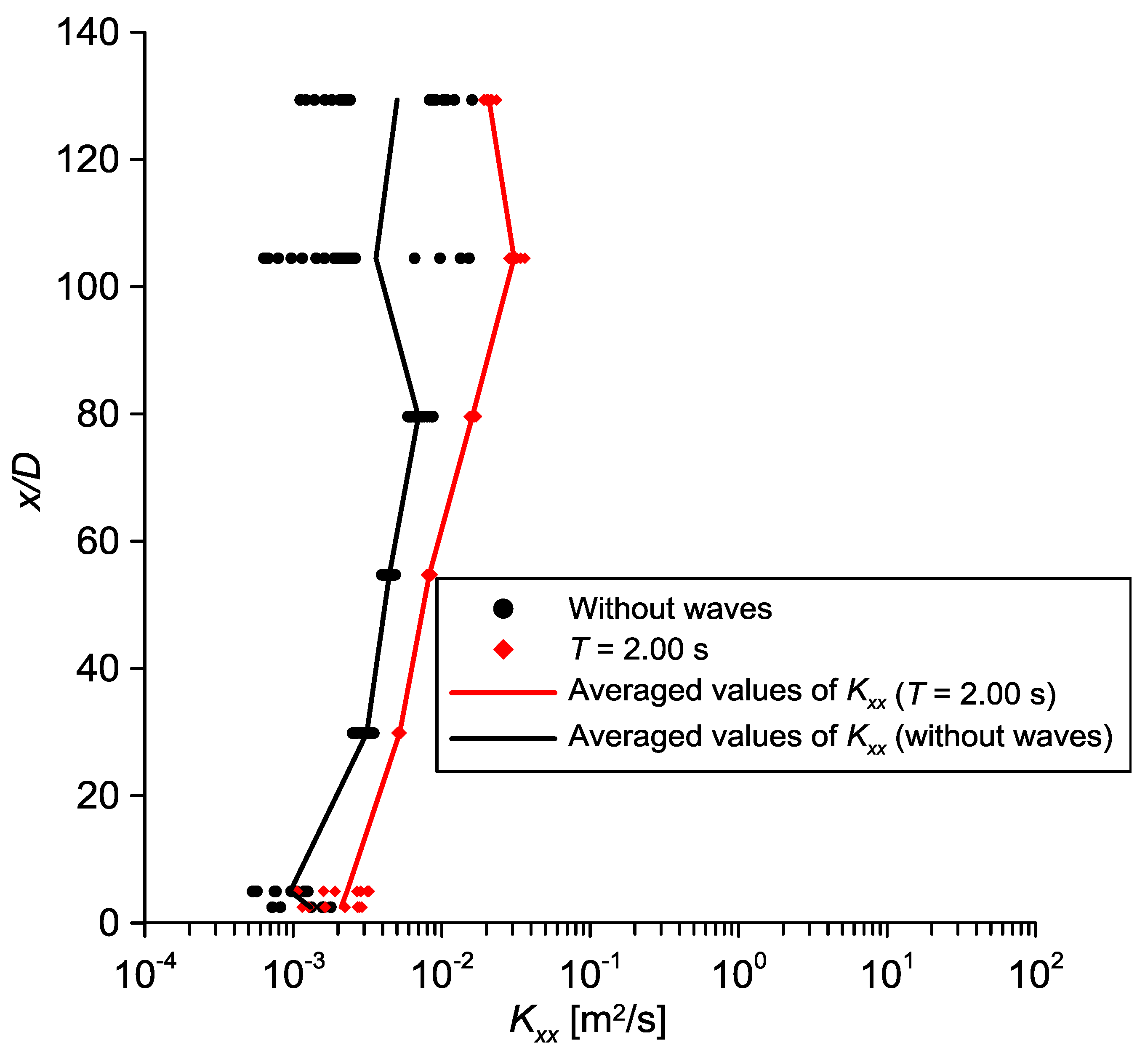
Figure 14 shows the values of the streamwise turbulent diffusion coefficient Kxx of each cross section of the jet as a function of the distance from the nozzle. The dots in Figure 14 represent individual estimates at all y positions in the analysed cross sections and the lines represent their averages.
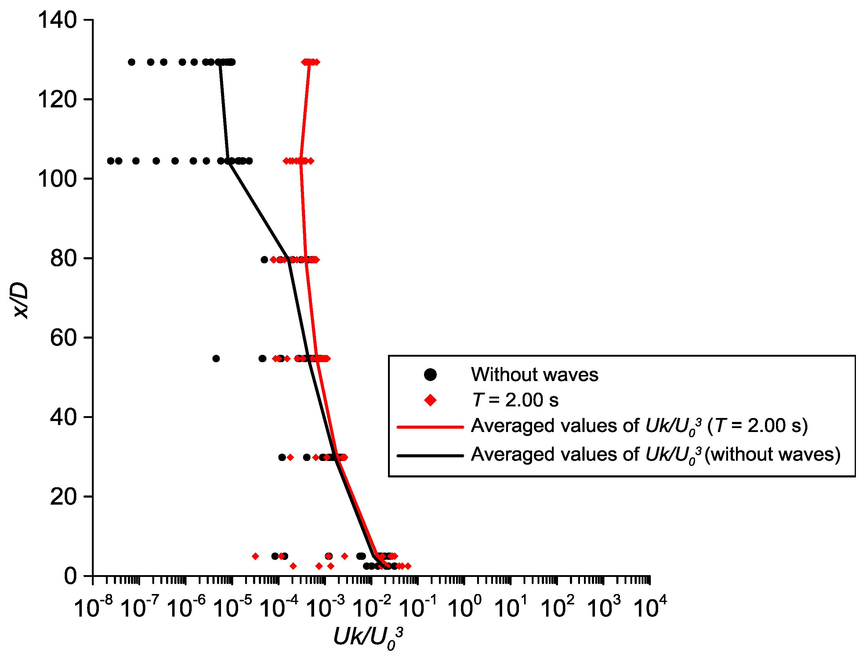
Figure 15 shows the values of Uk of each cross section of Run 1 of Table 1 and of the same jet without waves. The dots in Figure 13 represent individual estimates at all y positions in the analysed cross sections with the lines representing the averages.
For the sake of brevity, Figure 14 and Figure 15 show the data of Run 1 of Table 1 and of the same jet without waves, but the results are confirmed also by the other analysed configurations with waves. The averaged values of Figure 14 and Figure 15 demonstrate that the streamwise diffusion coefficient Kxx and the streamwise advection of the jet with waves are greater than those of the same jet issued into still water. Furthermore, the differences of values of Kxx for the jets with and without waves increase with the distance from the nozzle.
In any case, the advection term is of the same order of magnitude at a distance from the nozzle of O(<Lw), i.e., in the jet region where the initial jet momentum is of the order of the wave-induced momentum. These results are better shown in Figure 14 and Figure 15 with the lines of averaged values, which enable us to quantify the difference between the cases with and without waves. In the region closer to the nozzle, the longitudinal advection terms of jets issued into a wave environment or into still water are comparable, demonstrating that the wave action is less pronounced. From the experimental results presented above, it is possible to conclude that the presence of waves increases both the diffusion and advection processes in the longitudinal direction in the jet region where the wave-induced momentum is greater than the initial jet momentum.
4. Conclusions
Turbulent jets flowing in currents or still water have been widely examined because of their relevance to many environmental conditions. This study examines turbulent nonbuoyant jets issued into a wave environment. The main conclusions can be summarised as follows:
- The analysis of the time-averaged and phase-averaged velocity vectors shows that the flow pattern resembles that of a jet discharged into a cross-current when the wave horizontal velocity dominates and that of a co-stream jet or jet in opposing flow when the vertical wave velocity dominates. Furthermore, the jet experiences an enlargement of its area when waves are present compared with the same jet in still water, which suggests an enhancement of the dilution and, therefore, a positive effect of the wave motion during the initial mixing processes. The velocity profiles of jets discharged in a wave environment are even flatter and wider than those of the same jet discharged in a stagnant environment.
- The analysis of the turbulent kinetic energy k nondimensionalised by U0 shows that close to the nozzle, specifically when x << Lw, the values are similar with and without waves, indicating that the impact of the waves on the turbulent kinetic energy is small. In this region it is possible to affirm that the turbulence is dominated by the jet and, therefore, this is a region with jet-generated shear. Farther from the nozzle, i.e., when x is closer to or greater than Lw, the values of k are higher with the presence of waves. In this region the turbulence of the jet is also affected by the waves. Furthermore, in the case of the jet with waves, O(k) is almost constant in the upper region, demonstrating that the waves feed the jet turbulence. On the contrary, in the case of the absence of waves, the values of k reduce at higher distance from the nozzle.
- The values of the mean axial velocity Uc normalised by the jet exit velocity U0 show that the configurations analysed in the present paper are well fitted by the classic literature laws for the measurement points in the jet’s fully developed region where the wave effect is not pronounced.
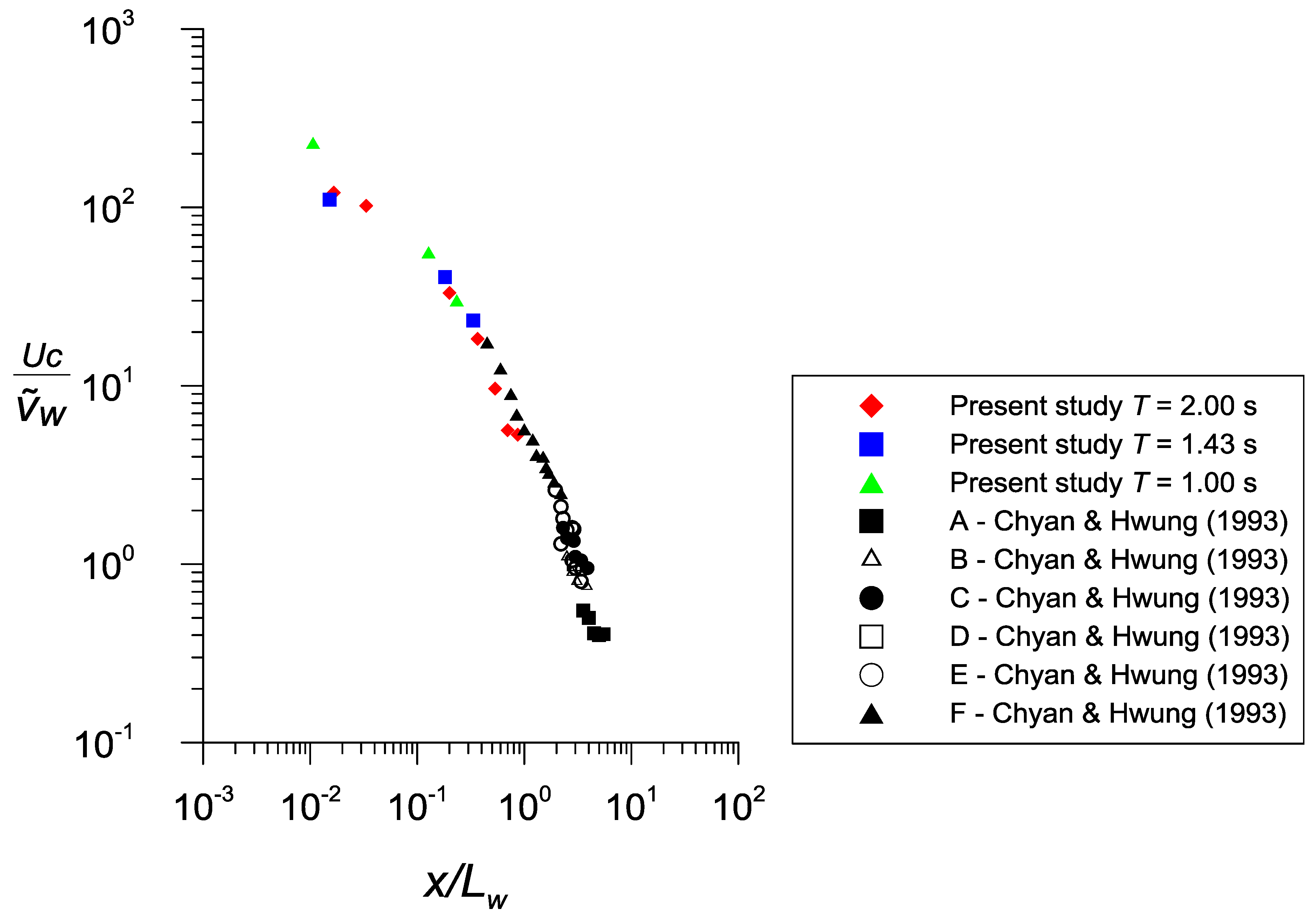
- The experimental data agree with Chyan and Hwung’s [27] law of the dimensionless Uc velocity as a function of x/Lw.
- Using the analogy between the equation of the turbulent transport of a solute concentration and the equation of the turbulent kinetic energy, the jet net dispersion coefficients have been evaluated. In contrast to the case of jets in still water, in the runs with waves, the streamwise turbulent diffusion is increased.
- The presence of waves increases both the diffusion and advection processes of the jet in the longitudinal direction, mainly in the region dominated by the wave-induced momentum, i.e., at distance from the nozzle greater than the length scale Lw.
Supplementary Materials
The following are available online at https://www.mdpi.com/2073-4441/10/4/522/s1. The two movies depict Run 1 of Table 1 of the paper (file jet_with_waves_run_1_Mossa.avi) and the same jet issued into still water (file jet_in_still_water.avi). A dye called Rhodamine B (C28H31ClN2O3) was used to visualize the jet flow pattern.
Author Contributions
M.M. conceived the experimental set up and carried out the experiments; both authors contributed to analysis of the data, writing of the paper, and discussions and review of the manuscript.
Funding
Peter Davies acknowledges the support of the UK Engineering and Physical Sciences Research Council (Grant EP/G066124/1).
Conflicts of Interest
The authors declare no conflict of interest.
References
- Mossa, M. Field measurements and monitoring of wastewater discharge in sea water. Estuar. Coast. Shelf Sci. 2006, 68, 509–514. [Google Scholar] [CrossRef]
- De Serio, F.; Mossa, M. A laboratory study of irregular shoaling waves. Exp. Fluids 2013, 54, 1536. [Google Scholar] [CrossRef]
- Ben Meftah, M.; De Serio, F.; Malcangio, D.; Mossa, M.; Petrillo, A.F. Experimental study of a vertical jet in a vegetated crossflow. J. Environ. Manag. 2015, 164, 19–31. [Google Scholar] [CrossRef] [PubMed]
- Armenio, E.; De Serio, F.; Mossa, M. Analysis of data characterizing tide and current fluxes in coastal basins. Hydrol. Earth Syst. Sci. 2017, 21, 3441. [Google Scholar] [CrossRef]
- De Serio, F.; Mossa, M. Environmental monitoring in the Mar Grande basin (Ionian Sea, Southern Italy). J. Environ. Sci. Pollut. Res. 2016, 23, 12662–12674. [Google Scholar] [CrossRef] [PubMed]
- List, E.J. Turbulent jets and plumes. Annu. Rev. Fluid Mech. 1982, 14, 189–212. [Google Scholar] [CrossRef]
- Davies, P.A.; Valente Neves, M.J. Recent Research Advances in the Fluid Mechanics of Turbulent Jets and Plumes; NATO ASI Series, Series E: Applied Sciences; Springer Science & Business Media: New York, USA, 2012; Volume 255, ISBN 978-94-010-4396-0. [Google Scholar] [CrossRef]
- Lee, J.H.W.; Chu, V.H. Turbulent Jets and Plumes—A Lagrangian Approach; Kluwer Academic Publishers: Dordrecht, the Netherlands, 2003; ISBN 1402075200. [Google Scholar]
- Wood, I.R.; Bell, R.G.; Wilkinson, D.L. Ocean Disposal of Wastewater; Advanced Series on Ocean Engineering; World Scientific: Singapore, 1993; Volume 8. [Google Scholar]
- Roberts, P.J.W.; Salas, H.J.; Reiff, F.M.; Libhaber, M.; Labbe, A.; Thomson, J.C. Marine Wastewater Outfalls and Treatment Systems; IWA Publishing: Colchester, UK, 2010; ISBN 1843391899. [Google Scholar]
- Tate, P.M.; Scaturro, S.; Cathers, B. Marine outfalls. In Springer Handbook of Ocean Engineering; Dhanak, M.R., Xiros, M.I., Eds.; Springer: Cham, Switzerland; Berlin, Germany, 2016; pp. 711–740. ISBN 978-3-319-16648-3. [Google Scholar]
- Jirka, G.H.; Harleman, D.R.F. Stability and mixing of a vertical plane buoyant jet in confined depth. J. Fluid Mech. 1979, 94, 275–304. [Google Scholar] [CrossRef]
- Papanicolaou, P.N.; List, E.J. Investigation of round vertical turbulent buoyant jets. J. Fluid Mech. 1988, 195, 341–391. [Google Scholar] [CrossRef]
- Atkinson, J.F.; Wolcott, S.B. Interfacial mixing induced by mean shear and an oscillating grid. J. Hydraul. Eng. 1990, 116, 397–413. [Google Scholar] [CrossRef]
- Smith, S.H.; Mungal, M.G. Mixing, structure and scaling of the jet in crossflow. J. Fluid Mech. 1998, 357, 83–122. [Google Scholar] [CrossRef]
- Jirka, G.H. Large scale flow structures and mixing processes in shallow flows. J. Hydraul. Res. 2001, 39, 567–573. [Google Scholar] [CrossRef]
- Shuto, N.; Ti, L.H. Wave effects on buoyant plumes. In Proceedings of the 14th Conference on Coastal Engineering, Copenhagen, Denmark, 24–28 June 1974; pp. 2199–2209. [Google Scholar]
- Ger, A.M. Wave effects on submerged buoyant jets. In Proceedings of the 18th IAHR, Cagliari, Italy, 10–14 September 1979; pp. 295–300. [Google Scholar]
- Sharp, J.J. The effects of waves on buoyant jets. Proc. Inst. Civ. Eng. 1986, 81, 471–475. [Google Scholar]
- Rajaratnam, N. Turbulent Jets; Elsevier Scientific Publishing Company: Amsterdam, The Netherlands; Oxford, UK; New York, NY, USA, 1976. [Google Scholar]
- Fischer, H.B.; List, E.J.; Koh, R.C.Y.; Imberger, J.; Brooks, N.H. Mixing in Inland and Coastal Waters; Academic Press: New York, NY, USA, 1979. [Google Scholar]
- Peregrine, D.H. Interaction of water waves and currents. Adv. Appl. Mech. 1976, 16, 9–117. [Google Scholar]
- Roberts, P.J.W. Ocean outfall dilution: Effects of currents. J. Hydraul. Div. 1980, 106, 769–782. [Google Scholar]
- Ismail, N.M.; Wiegel, R.L. Opposing wave effect on momentum jets spreading rate. J. Waterw. Port Coast. Ocean Eng. 1983, 109, 465–483. [Google Scholar] [CrossRef]
- Chin, D.A. Influence of surface waves on outfall dilution. J. Hydraul. Eng. 1987, 113, 1006–1017. [Google Scholar] [CrossRef]
- Yoon, S.B.; Liu, P.L.-F. Effects of opposing waves on momentum jets. J. Waterw. Port Coast. Ocean Eng. 1990, 116, 545–557. [Google Scholar] [CrossRef]
- Chyan, J.-M.; Hwung, H.-H. On the interaction of a turbulent jet with waves. J. Hydraul. Res. 1993, 31, 791–810. [Google Scholar] [CrossRef]
- Koole, R.; Swan, C. Measurements of a 2-D non-buoyant jet in a wave environment. Coast. Eng. 1994, 24, 151–169. [Google Scholar] [CrossRef]
- Calabrese, M.; Di Natale, M. Diffusione di un getto liquido sommerso in presenza di un moto ondoso stazionario. In Proceedings of the XXIV Convegno di Idraulica e Costruzioni Idrauliche, Napoli, Italy, 20–22 September 1994; Volume I, pp. 241–254. (In Italian). [Google Scholar]
- Nash, J.D.; Jirka, G.H. Buoyant surface discharges into unsteady ambient flows. Dyn. Atmos. Oceans 1996, 24, 75–84. [Google Scholar] [CrossRef]
- Wu, S.; Rajaratnam, N.; Katopodis, C. Oscillating vertical plane turbulent jet in shallow water. J. Hydraul. Res. 1998, 36, 229–234. [Google Scholar] [CrossRef]
- Mossa, M. Experimental study on the interaction of non-buoyant jets and waves. J. Hydraul. Res. 2004, 42, 13–28. [Google Scholar] [CrossRef]
- Mossa, M. Behavior of non-buoyant jets in a wave environment. J. Hydraul. Eng. 2004, 130, 704–717. [Google Scholar] [CrossRef]
- Chin, D.A. Model of buoyant-jet-surface-wave interaction. J. Waterw. Port Coast. Ocean Eng. 1988, 114, 331–345. [Google Scholar] [CrossRef]
- Davies, P.A.; Mofor, L.A.; Valente Neves, M.J. Comparisons of remotely sensed observations with modeling predictions for the behaviour of wastewater plumes from coastal discharges. Int. J. Remote Sens. 1997, 18, 1987–2019. [Google Scholar]
- Lee, J.H.W.; Wilkinson, D.L.; Wood, I.R. On the head-discharge relation of a “duckbill” elastomer check valve. J. Hydraul. Res. 2001, 39, 619–627. [Google Scholar] [CrossRef]
- Cuthbertson, A.J.S.; Malcangio, D.; Davies, P.A.; Mossa, M. The influence of a localised region of turbulence on the structural development of a turbulent, round, buoyant jet. Fluid Dyn. Res. 2006, 38, 683–698. [Google Scholar] [CrossRef]
- Mossa, M.; De Serio, F. Rethinking the process of detrainment: Jets in obstructed natural flows. Sci. Rep. 2016, 6, 39103. [Google Scholar] [CrossRef] [PubMed]
- Mossa, M.; Ben Meftah, M.; De Serio, F.; Nepf, H.M. How vegetation in flows modifies the turbulent mixing and spreading of jets. Sci. Rep. 2017, 7, 6587. [Google Scholar] [CrossRef] [PubMed]
- Hussain, A.K.M.F.; Reynolds, W.C. The mechanics of an organized wave in turbulent shear flow. J. Fluid Mech. 1970, 41, 241–258. [Google Scholar] [CrossRef]
- Svendsen, I.A. Analysis of surf zone turbulence. J. Geophys. Res. 1987, 92, 5115–5124. [Google Scholar] [CrossRef]
- Tanino, Y.; Nepf, H.M. Lateral dispersion in random cylinder arrays at high Reynolds number. J. Fluid Mech. 2008, 600, 339–371. [Google Scholar] [CrossRef]
- Le Méhauté, B. An Introduction to Hydrodynamics and Water Waves; Water Wave Theories, II, TR ERL 118-POL-3-2; U.S. Department of Commerce, ESSA: Washington, DC, USA, 1969.
- Albertson, M.L.; Dai, Y.B.; Jensen, R.A.; Rouse, H. Diffusion of submerged jets. Trans. ASCE 1950, 115, 639–664. [Google Scholar]
- Corrsin, S.; Uberoi, M.S. Further experiments on the flow and heat transfer in a heated turbulent air jet. NACA Rep. 1950, 998, 1–17. [Google Scholar]
- Wygnanski, I.J.; Fiedler, H.E. Some measurements in the self-preserving jet. J. Fluid Mech. 1969, 38, 577–612. [Google Scholar] [CrossRef]
Figure 1.
Typical release of jets in wave environment. The discharge region is located offshore of the surf zone.
Figure 1.
Typical release of jets in wave environment. The discharge region is located offshore of the surf zone.

Figure 2.
Drawing of the experimental setup.

Figure 3.
Jet defining drawing.

Figure 4.
Sketch of the LDA system with the wave gauge, the AD/DA board and the process computer.

Figure 5.
Experimental apparatus: (a) LDA probe; (b) Dantec FVA signal processor and process computer; (c) Laser Coherent Innova and Dantec 2D Fibre Flow optics; (d) process computer with an AD/DA board for the wavemaker control; (e) a part of the wave channel where the jets were discharged; (f) the wavemaker.

Figure 6.
Flow patterns of the jet issued into still water and a time sequence of images of the same jet in a wave flow field of period T at different wave phases separated by T/8 (Test 1 of Table 1). The grid helps to show the jet oscillations.
Figure 6.
Flow patterns of the jet issued into still water and a time sequence of images of the same jet in a wave flow field of period T at different wave phases separated by T/8 (Test 1 of Table 1). The grid helps to show the jet oscillations.

Figure 7.
Phase-averaged flow patterns of velocity vectors of Run 1 of Table 1 acquired at a time rate of one-quarter of the wave period: (a) wave trough to crest passage; (b) under the wave crest; (c) wave crest to trough passage; (d) under the wave trough.
Figure 7.
Phase-averaged flow patterns of velocity vectors of Run 1 of Table 1 acquired at a time rate of one-quarter of the wave period: (a) wave trough to crest passage; (b) under the wave crest; (c) wave crest to trough passage; (d) under the wave trough.

Figure 8.
Time-averaged velocity vectors of Run 1 of Table 1 and of the same jet in still water.
Figure 8.
Time-averaged velocity vectors of Run 1 of Table 1 and of the same jet in still water.

Figure 9.
Values of k0.5/U0 with the definition of the region with jet-generated turbulence (at the bottom) and the region with jet–wave-generated turbulence (at the top).
Figure 9.
Values of k0.5/U0 with the definition of the region with jet-generated turbulence (at the bottom) and the region with jet–wave-generated turbulence (at the top).

Figure 10.
Values of U0/Uc along the jet mean axis.

Figure 11.
Distribution of the dimensionless values of Uc along the dimensionless distance.

Figure 12.
Values of Kxx of Run 1 of Table 1 and of the same jet without waves.
Figure 12.
Values of Kxx of Run 1 of Table 1 and of the same jet without waves.

Figure 13.
Values of Uk of Run 1 of Table 1 and of the same jet without waves.
Figure 13.
Values of Uk of Run 1 of Table 1 and of the same jet without waves.

Figure 14.
Values of Kxx of Run 1 of Table 1 and of the same jet without waves with lines of the averaged values of each cross section.
Figure 14.
Values of Kxx of Run 1 of Table 1 and of the same jet without waves with lines of the averaged values of each cross section.

Figure 15.
Values of Uk of Run 1 of Table 1 and of the same jet without waves with lines of the averaged values of each cross section.
Figure 15.
Values of Uk of Run 1 of Table 1 and of the same jet without waves with lines of the averaged values of each cross section.


Table 1.
Main characteristics of the jet configurations with waves.
| Test with Waves | H [cm] | L [m] | T [s] | H/L | h/L | [m/s] | Lw [m] |
|---|---|---|---|---|---|---|---|
| 1 | 4.20 | 5.10 | 2.00 | 0.0082 | 0.16 | 0.039 | 0.31 |
| 2 | 4.40 | 3.05 | 1.43 | 0.014 | 0.26 | 0.036 | 0.33 |
| 3 | 4.13 | 1.56 | 1.00 | 0.027 | 0.51 | 0.026 | 0.47 |
Table 2.
Main flow conditions and instrumentation used by the authors of the previous investigations.
Table 2.
Main flow conditions and instrumentation used by the authors of the previous investigations.
| Authors | Runs | Jet Diameter/Jet Slot | Fluid | Wave Period | h/L | U0 | Velocity Measurements |
|---|---|---|---|---|---|---|---|
| Albertson et al. [44] | All | From 0.08 cm to 2.54 cm | Air | - | - | From 12.19 m/s to 54.86 m/s | Hypodermic needle with water differential manometer or sensitive two-liquid gauge, midget spoke-vane anemometer |
| Corrsin and Uberoi [45] | All | 2.54 cm | Air | - | - | From 19.81 m/s to 35.05 m/s | Hypodermic needle total-head tube, Chromel-Alumen thermocouple (for mean velocity) and hot-wire anemometer (turbulent velocity components) |
| Wygnanski and Fiedler [46] | All | 2.64 cm | Air | - | - | From 51 m/s to 72 m/s | Constant-temperature anemometers and linearisers with standard hot wires |
| Chyan and Hwung [27] | A | 2.3 mm | Water | 1.16 s | 0.1470 | 83.7 cm/s | LDA |
| B | 2.3 mm | 0.85 s | 0.2251 | 84.7 cm/s | |||
| C | 2.3 mm | 0.75 s | 0.2731 | 83.6 cm/s | |||
| E | 2.3 mm | 0.64 s | 0.3598 | 83.2 cm/s | |||
| F | 2.3 mm | 0.52 s | 0.5343 | 83.4 cm/s | |||
| G | 2.3 mm | - | - | 82.5 cm/s | |||
| H | 5.0 mm | - | - | 62.4 cm/s |
© 2018 by the authors. Licensee MDPI, Basel, Switzerland. This article is an open access article distributed under the terms and conditions of the Creative Commons Attribution (CC BY) license (http://creativecommons.org/licenses/by/4.0/).
Share and Cite
MDPI and ACS Style
Mossa, M.; Davies, P.A. Some Aspects of Turbulent Mixing of Jets in the Marine Environment. Water 2018, 10, 522. https://doi.org/10.3390/w10040522
AMA Style
Mossa M, Davies PA. Some Aspects of Turbulent Mixing of Jets in the Marine Environment. Water. 2018; 10(4):522. https://doi.org/10.3390/w10040522
Chicago/Turabian StyleMossa, Michele, and Peter A. Davies. 2018. "Some Aspects of Turbulent Mixing of Jets in the Marine Environment" Water 10, no. 4: 522. https://doi.org/10.3390/w10040522
Note that from the first issue of 2016, this journal uses article numbers instead of page numbers. See further details here.