Seasonal and Interannual Variability in Coastal Circulations in the Northern South China Sea


1
Institute of Physical Oceanography, Ocean College, Zhejiang University, Zhoushan 316021, China
2
State Key Laboratory of Satellite Ocean Environment Dynamics, Second Institute of Oceanography, State Oceanic Administration, Hangzhou 310000, China
*
Author to whom correspondence should be addressed.
Water 2018, 10(4), 520; https://doi.org/10.3390/w10040520
Submission received: 13 March 2018
/
Revised: 15 April 2018
/
Accepted: 19 April 2018
/
Published: 21 April 2018
(This article belongs to the Section Hydrology)
Abstract
:Seasonal cycle and interannual variability in coastal circulations in the northern South China Sea (NSCS) are investigated using satellite altimeter data from March 1993 to September 2016. Altimeter-derived velocity anomalies are in good agreement with acoustic Doppler current profilers (ADCP) observations at an adjacent location. Along-shelf volume transport anomalies in the NSCS indicate northeastward transports from mid-spring to summer and southwestward transports from mid-autumn to winter, which are consistent with previous studies in this region. According to convergence and divergence in the target control volumes, cross-shelf volume transports are estimated as the differences between two neighboring along-shelf volume transport anomalies, with the assumption that long-term mean along-shelf volume transports at each cross-sections are identical. The results show onshore transports in mid-autumn and offshore transports in early summer. The comparison between altimeter-derived and ADCP-estimated cross-shelf volume transports is encouraging, especially when the region has relatively low mesoscale activities and a low freshwater input. Reconstructed cross-shelf volume transports through multiple linear regression reveal that seasonal harmonics is the primary force in driving cross-shelf volume transports in the NSCS, while wind and El Niño have secondary effects on controlling cross-shelf volume transports in different regions. The present study helps to quantify the long-term coastal circulations, especially cross-shelf volume transports, based on altimeter data, which has important implications on the dynamics in coastal regions where observational data is limited.
1. Introduction
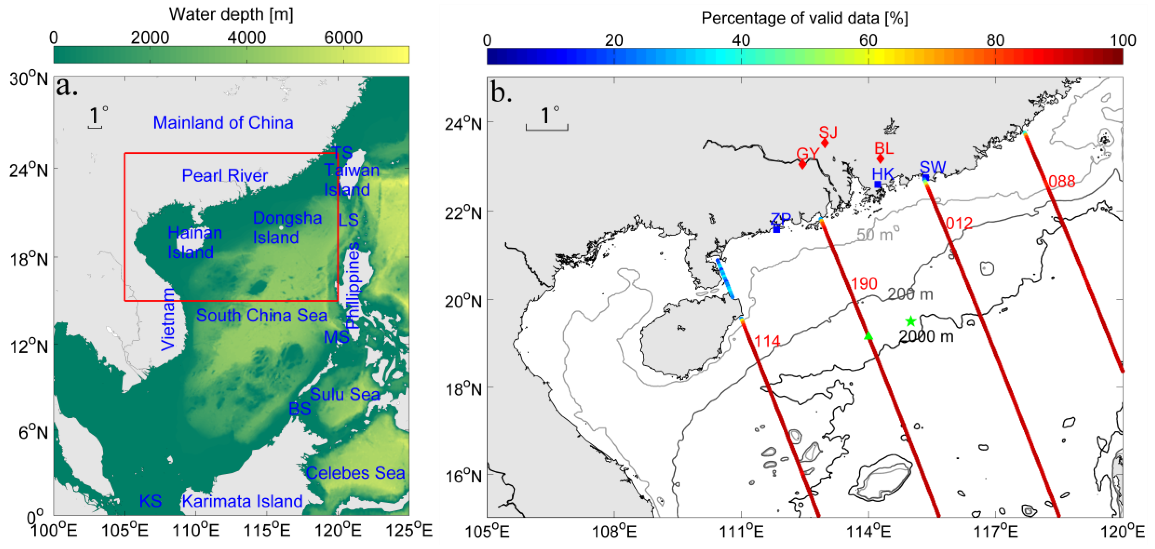
The South China Sea (SCS) is the largest marginal sea in the northwest Pacific, with a total area of 3.5 million km2 (Figure 1a). It connects the East China Sea, Pacific, Sulu Sea, Java Sea via the Taiwan Strait (TS), the Luzon Strait (LS), the Mindoro Strait (MS) and the Balabac Strait (BS), and the Karimata Strait (KS), respectively [1,2]. The northern South China Sea (NSCS) has a wide continental shelf adjacent to southern China, where the 200 m isobath (considered to be the continental shelf break) is typically beyond 100 km from the coast. The Pearl River, the third largest river system in China, delivers more than 3.5 × 10¹¹ m3 of freshwater and 8.5 × 10⁷ tons of sediment every year to the NSCS continental shelf through three major tributaries: the Xijiang, Beijiang, and Dongjiang [3]. The isobaths in the NSCS are approximately parallel to the coastline except in the areas located between Hainan Island and the Luzon Strait, around 350 km southeast off the Pearl River Estuary (Figure 1b).
Using in situ observations, numerical simulations or satellite altimetry, extensive researches were conducted to investigate seasonal and interannual circulation and volume transports in the SCS (e.g., [4,5,6,7,8,9,10]). Fang, et al. [10] found that seawater in the SCS permanently flows to the Indonesian sea in winter from one year of observation of moored acoustic Doppler current profiler (ADCP) data from December 2007 to November 2008. The maximum flow through the Karimata Strait can exceed 5 Sv (1 Sv = 1.0 × 10⁶ m3/s). The annual volume transports through the Luzon Strait, the Taiwan Strait, the Sunda Shelf and the Mindoro Strait are −4.5, 2.3, 0.5, and 1.7 Sv, respectively, based on the quasi-global high-resolution Hybrid Coordinate Ocean Model (HYCOM) study [9]. The first three modes show significant (accounting for 57% of the total variance) seasonal features in the SCS based on empirical orthogonal function (EOF) analysis from 11-year sea surface height anomaly (SSHA) data from a satellite altimeter [7]. The volume transports through the Luzon Strait is very important and has received much attention recently. Research shows that the annual mean transport through the Luzon Strait is 2.4–4.8 Sv [4,5,6,8,9] and reaches its seasonal minimum in summer and maximum in winter [4,5].
Because of complex ocean dynamics (e.g., the East Asia monsoon [11], Kuroshio intrusion [12], the Pearl River plume [13], mesoscale eddy activity [14]) in the NSCS, most previous studies have focused on circulation or volume transports through the straits in the SCS. Research into the NSCS has mainly depended on in situ observations [15,16] with the spatial distribution being uneven and the time distribution being intermittent. We lack a long-term study of the overall dynamics in the NSCS. Zhu, et al. [16] investigated a 22-year cross-track (along-shelf direction) volume transport in the NSCS by combining five pressure-recording inverted echo sounders data taken from a two-year period and empirical modes. They found that the mean transport is 1.6 Sv to the southwest; the peak transports are 3.6 Sv to the northeast in July, and 7.3 Sv to the southwest in December. Most of them have not investigated the cross-shelf volume transport in the NSCS adequately.
The cross-shelf volume transport plays an important role in linking the shelf circulation. It controls the fates of the freshwater and sediment delivered by the nearby rivers, transferring nutrients, contaminants, and carbon from coastal areas to the shelf regions, thus influencing the ecosystem over the shelf. Although the cross-shelf volume transport is extremely significant in determining the physical environments and biogeochemical cycles over the shelf regions, unfortunately, relevant research focusing on quantifying a long-term cross-shelf volume transport is lacking in the NSCS. This is partially due to the relatively small magnitudes and high spatial variations of the cross-shelf velocity compared with the along-shelf velocity. It may also be because of the shortage of in situ observations and the complexity of the ocean dynamics in the NSCS.
Since the 1990s, satellite altimetry has provided us with an extremely useful approach for achieving long-term observation in global sea surface height (SSH). With the developments of the tide mode, atmosphere mode, and waveform retracking, satellite altimetry has been successfully applied to investigate the sea level variability and the geostrophic current in coastal oceans [17,18,19]. Sea level anomaly (SLA) and subsequently derived geostrophic velocity are in good agreement with in situ observations (e.g., tide gauge (TG), ADCP), which shows that a satellite altimeter is capable of gaining sea level information and thus obtaining geostrophic current status [17,18,20,21,22,23].
In this study, we use 24-year altimeter data to obtain along-shelf and cross-shelf circulation in the NSCS. Along-shelf volume transport anomalies are calculated by multiplying velocity anomalies with the cross-section area. Then, cross-shelf volume transports are estimated as the differences between two neighboring along-shelf volume transport anomalies based on convergence and divergence in the target control volumes with the assumption that the long-term mean along-shelf volume transports at each of the cross-sections are identical. We analyzed several potential factors that may affect the shelf circulation in the NSCS, for example, wind, El Niño, Pearl River discharge, and Kuroshio intrusion through the Luzon Strait. We also reconstruct the cross-shelf volume transport based on the important external forces and investigate their relative contributions. The limitations of present assumptions and calculations are discussed subsequently. This research provides us with a good opportunity to quantify variation and mechanisms of coastal circulations in the NSCS, which may be useful for us to better understand and study coastal ecosystems.
2. Data and Methods
2.1. Along-Track Sea Level Anomaly (SLA)
The altimeter data (1 Hz along-track SLA) used in the present study were processed and distributed by the Center for Topographic studies of the Ocean and Hydrosphere (CTOH, http://ctoh.legos.obs-mip.fr) via combining Topex/Poseidon (TP: 1992–2002), Jason-1 (J1: 2002–2008) and Jason-2 (J2: 2008–2016) missions. Along-track SLA data from March 1993 to September 2016 have applied geophysical corrections (e.g., atmospheric loading effects correction and tides mode) [21] and have the sea surface information with a 9.9156 days repeat.
Four ascending tracks (track 088, 012, 190, and 114) were used here to investigate cross-shelf volume transports as they were almost perpendicular to the coastline in the NSCS (Figure 1). SLA data at each location that exceeded three sample standard deviations were eliminated. The ratio of valid data increased monotonically and dramatically as the offshore distance increased. As such, we chose points with higher than 75% valid data to remove non-robust points close to the coast [20]. This data was then referred as a full SLA time series.
Seasonal cycle of SLA (SLASC) time series was estimated as the sum of annual and semi-annual harmonics by applying harmonic analysis to the full SLA in the NSCS:
where a, b, c, d are harmonic coefficients, 2π/(365.25 days), 4π/(365.25 days) are annual frequency and semi-annual frequency, respectively, and t is time in days.
Low frequency components of the SLA time series were calculated by applying a 120-day low-pass filter to the full SLA time series [23]. The differences between the low-frequency component and seasonal cycle of SLA are the interannual variability of SLA. Similar methods were applied to other data subsequently (e.g., geostrophic velocity anomalies, wind stress, Pearl River discharge) to obtain the interannual variability in each parameter after their pre-processes.
2.2. Geostrophic Velocities
Following [24,25], we applied a 12 points (about 75 km) linear regression to obtain cross-track geostrophic velocities in the NSCS:
where v is geostrophic velocities, g = 9.8 kg/m3 is gravitational acceleration, f is Coriolis parameter, h is the sea level anomaly, s is the along-track coordinate, and ∂h/∂s is the 12 points linear regression to SLA along the ground track. As the angle between the cross-track direction and 200 m isobath in this region is small (7°), we treated the along-shelf direction as being equivalent to the cross-track direction in our study. Although velocities vary vertically in the water column, the geostrophic velocities calculated here are the mean velocities in the near-surface layer. Velocities calculated based on the SLA data are geostrophic velocity anomalies, i.e., the differences between the instantaneous geostrophic velocities and the long-term mean values at this location. It is worth noting that the temporal average of geostrophic velocity anomalies at each location were slightly different from zero because of the linear regression process, hence, we further removed the mean values to obtain geostrophic velocity anomalies. The velocities calculated from full SLA data were referred as the full along-shelf velocity anomalies; we then used the method in Section 2.1 to obtain the interannual variability in geostrophic velocity anomalies.
2.3. Wind Data
Combining satellite, moored buoy, and model wind data, the Cross-Calibrated Muti-Platform (CCMP) synthesized gridded vector winds with a spatial resolution of 0.25° and a temporal resolution of 6 hours at a height of 10 m [26]. The wind data were downloaded from a Remote Sensing System (RSS, http://www.remss.com) and the along-shelf and cross-shelf wind stress components were computed thereafter [27]. In order to remove the subtidal motion effects and the match satellite Nyquist frequency, we followed the method proposed by Reference [20], by applying a 40-h low-pass filter and a 20-day low-pass filter to the wind stress time series as the pre-process. Then we used the method in Section 2.1 to obtain the interannual variability in wind stress. We applied an exponentially weighted running mean to the along-shelf and the cross-shelf wind stress time series because the influence of wind on the Ekman currents is not just the instantaneous effects of wind passing through but also must include the cumulative effects from before [28].
where and are wind stress magnitude in the along-shelf or cross-shelf direction after and before the exponentially weighted running mean are employed, respectively; R is the relaxation timescale to the maximize weighted-average wind stress and altimeter-derived velocities. We applied different R values to calculate the correlation and to find small differences among different R values, therefore, we chose R = 10 days in this study.
The along-shelf Ekman velocity was computed as follows [20]:
The wind-induced volume transport was calculated using [29]:
where is the along-shelf Ekman velocity, = 1025 kg/m3 is seawater density, DE is Ekman depth, f is Coriolis parameter, is water depth, Vx is cross-shelf volume transport, Vy is along-shelf volume transport, = 0.02 m2/s [21,30] is eddy viscosity, and are along-shelf and cross-shelf wind stress, respectively, h is the bathymetry. Specifically, as follows [31],
where is wind velocity at 10 m above the sea surface, = 7.292 × 10⁻⁵ is angular velocity of earth rotation, is latitude, and the average in the NSCS is about 64 m based on the average wind velocity in this region.
2.4. Additional Data
Research quality daily TG data were download from the University of Hawaii Sea Level Center (UHSLC, http://uhslc.soest.hawaii.edu). TG data were obtained from Shanwei (SW), Hong Kong (HK), and Zhapo (ZP). Detailed information about TG data is shown in Figure 1b and Table 1.
Moored ADCP was deployed from May 2015 to September 2016 at a location between ground track 012 and 190 (Figure 1b). To obtain the comparison with altimeter-derived velocities, near-surface (37 m) velocities measured by ADCP were used. Daily along-shelf ADCP velocity anomalies were computed by removing the mean value (0.119 m/s). Velocity anomalies were subsampled at 10-day intervals to match altimeter-derived velocity anomalies.
Monthly mean Pearl River discharge data from January 2002 to December 2015 were collected from the River and Sediment Bulletin of Ministry of Water Resources of the People’s Republic of China (MWR, http://www.mwr.gov.cn). Pearl River discharge is the sum of the runoff from three hydrological stations (HS): Gaoyao (GY) at Xijiang, Shijiao (SJ) at Beijiang, and Boluo (BL) at Dongjiang [13] (Figure 1b and Table 1).
Maps of the absolute dynamic topography (MADT) and UV maps of the geostrophic velocity anomalies data were provided by Archiving, Validation and Interpretation of Satellite Oceanographic data (AVISO, https://www.aviso.altimetry.fr) with a spatial resolution of 0.25° and a temporal resolution of 1 day. MADT data were used to calculate the index of Kuroshio intrusion to the SCS. The eddy kinetic energy (EKE) were estimated by and longitudinal and meridional geostrophic velocity anomalies (U′ and V′) as:
3. Results
3.1. Sea Level Anomalies
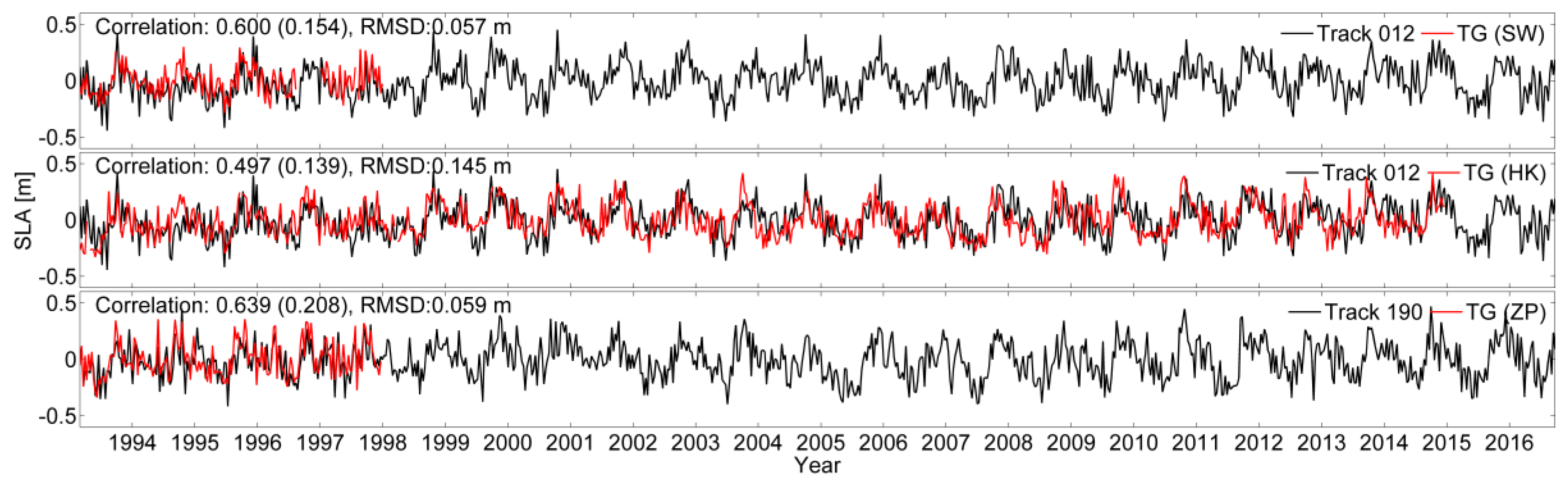
In order to evaluate the altimeter’s availability of obtaining SLA near the coast, we compare TG-measured SLA with the closest valid point (about 20 km off the coast) along the altimeter ground tracks (Figure 2). Correlation coefficients (95% confidence level (CL)) and root mean square differences (RMSDs) between the altimeter and TG data are shown in each panel. Comparisons show a good agreement between the TG and altimeter data, which reveals that altimeters are capable of gaining sea level information in the NSCS, even in regions near to the coast.
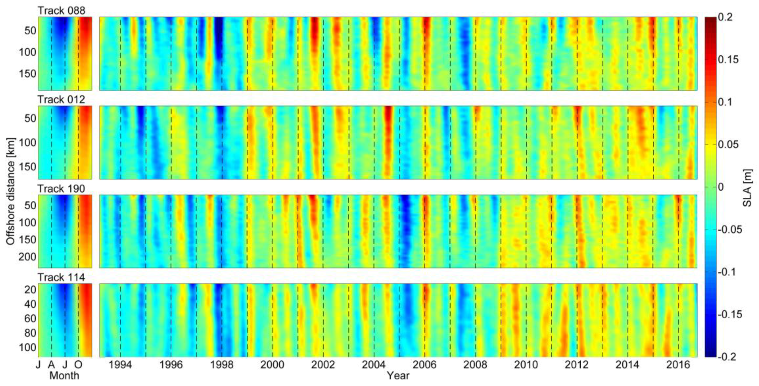
Seasonal cycles of SLA in the NSCS exhibit regular steric effects from seasonal cooling and heating [32], with negative values in spring and early summer and positive values in autumn and early winter (Figure 3). Here, we only plot the results within 200 m isobath to show the SLA variability in the NSCS shelf region. In the present study, we define the area within 200 m isobath as the shelf region, while the area deeper than 200 m as the offshore region. The variability in seasonal peaks are almost constant across the continental shelf, but the peaks progressively shift to earlier dates and get less strong offshore along track 088, 012, and 190. The seasonal cycles are dominated by the annual cycles as their amplitudes are about three times that of the semi-annual cycles. Monthly mean SLA variances (not shown) are relatively high near the coast and in the offshore area, which may be due to near-shore processes and the high frequency of mesoscale eddy activity [33], respectively.
The interannual variabilities in the SLA time series were generally low before 1999, with a minimum in 1997–1998 and apparently elevating after 1999 with peaks in 2001, 2004, and 2014. In contrast to the seasonal cycles of SLA, interannual variabilities have a lag effect in the offshore regions (not shown) compared with the shelf regions.
3.2. Geostrophic Velocity Anomalies
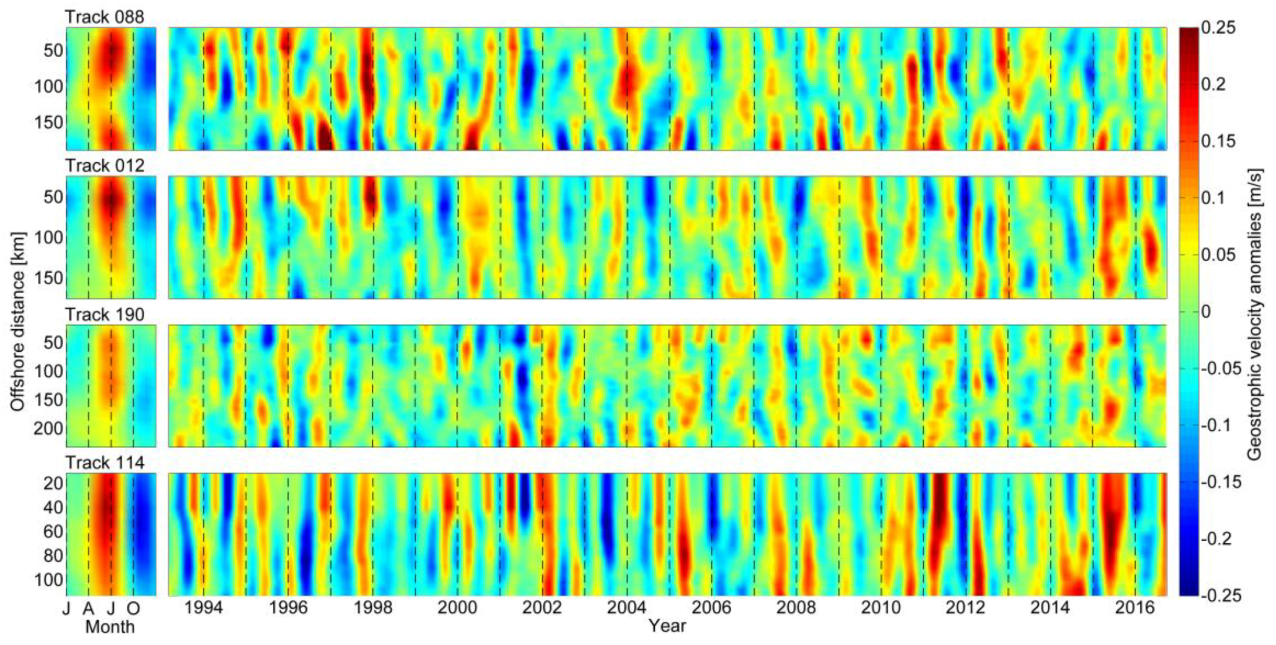
Seasonal cycles of geostrophic velocity anomalies are northeastward (positive values) from mid-spring to summer and southwestward (negative values) from mid-autumn to winter in the NSCS (Figure 4). The seasonal peaks of geostrophic velocity anomalies are much stronger in the shelf region and reach a low value near the shelf break except in track 088. Geostrophic velocity anomalies across ground track 088 have two peaks in the shelf region; this may be due to local terrain effects (the complex bathymetry of the Taiwan Bank where ground track 088 crosses).
Interannual variabilities in geostrophic velocity anomalies reach their extremum in 1994, 2001, 2007, and 2011. The interannual variability in track 012 and 190 are less consistent across the shelf compared to the other two tracks, which is presumably due to bathymetric effects or the influence by Pearl River diluted water.
The velocity variance in its smallest value is located at the shelf break region (at the bottom in Figure 4) in the four tracks. It increases towards the coast as well as in the offshore direction (not shown), while the former is presumably due to the impact of synoptic effects on a small time scale and the latter may be owing to stronger mesoscale processes.
3.3. Validation of Altimeter-Devied Geostrophic Velocity Anomalies
Along-shelf velocity anomalies at the nearest point along track 190 are compared with the velocity anomaly time series from moored ADCP (Figure 1b). It is worth pointing out that such comparisons are a challenge for the following reasons. Firstly, the altimeter data can only induce the geostrophic component of the near-surface velocity, while the ADCP measures both the geostrophic and ageostrophic components. Moreover, the distance between altimeter ground track and ADCP is about 111 km. Finally, water depth at the point along the altimeter ground track is about 800 m, while ADCP locates at 1600 m though the along-shelf velocity has little cross-shelf variation (Figure 4). Nevertheless, given the difficulties in obtaining long-term observational data, such comparisons still provide us with an opportunity to investigate the robustness of the altimeter-derived velocities in this region.
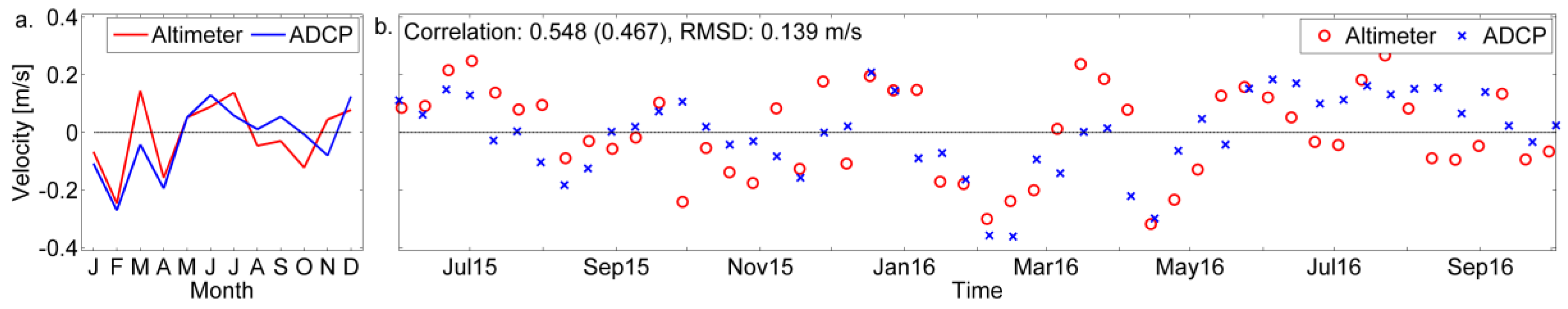
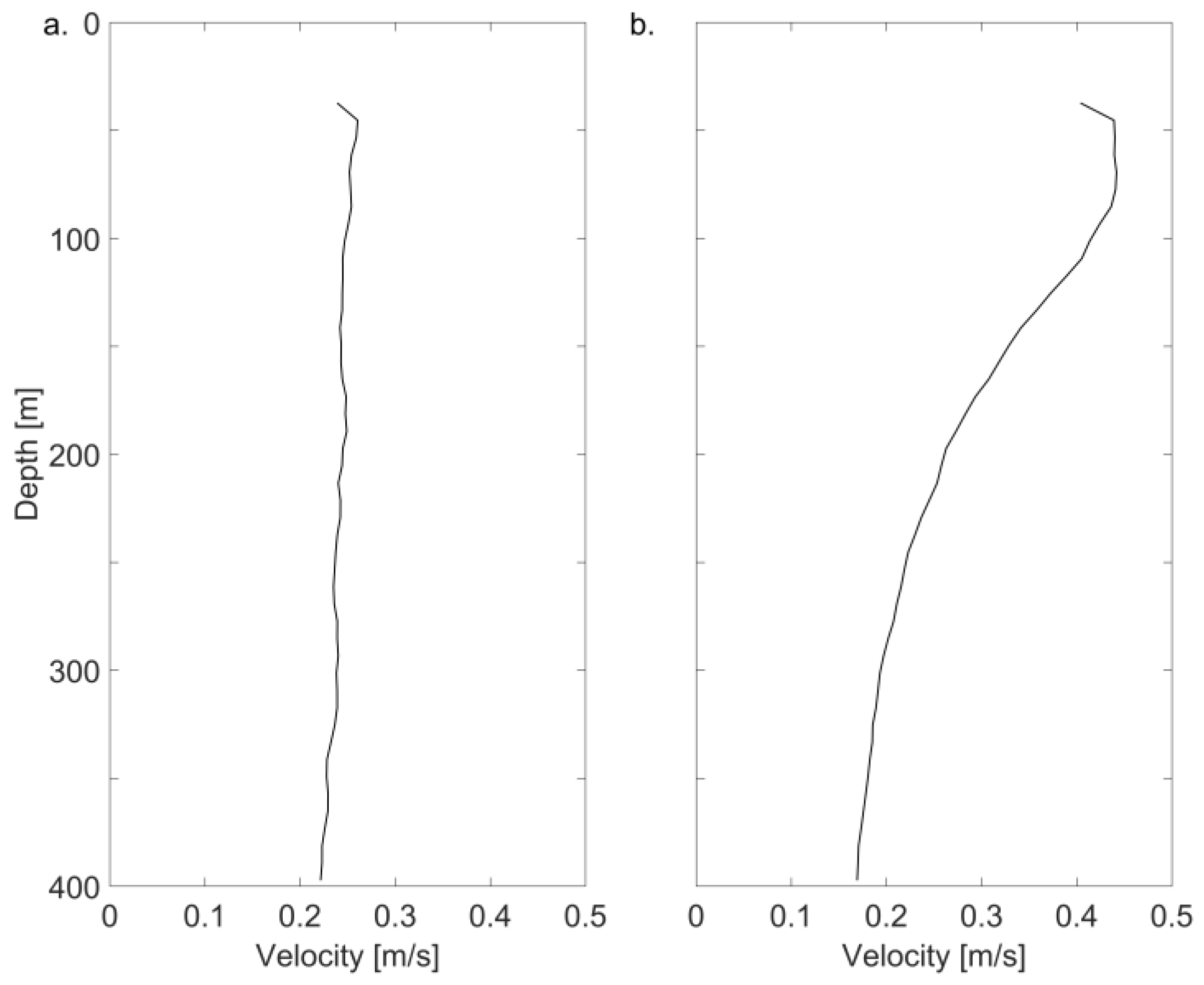
Figure 5 shows the comparison between the velocity anomalies time series from moored ADCP and altimeter data from May 2015 to September 2016. Unfortunately, the surface layer measurements of ADCP were contaminated during the whole period, so the top layer with valid data is 37 m. The monthly mean of the two-year altimeter-derived and ADCP-measured time series have the same seasonal cycle with some apparent differences (e.g., velocities in March or September). We emphasize that we can only calculate velocity anomalies using the sea level anomaly data. As such, although there are four months of velocity anomalies that have an opposite sign (Figure 5a), it does not necessarily imply that total flows are in the opposite direction. Future studies using absolute dynamic topography data would allow for better understanding of the full coastal transport in the NSCS region. Correlation coefficients (95% CL) of the altimeter-derived and ADCP-measured time series are 0.548 (0.467) and 0.755 (0.738) for the full- and low-frequency time series, respectively. The root mean square differences (RMSDs) between altimeter-derived and ADCP-measured velocities are 0.139 m/s and 0.065 m/s for the full- and low-frequency time series, respectively. The correlation coefficients and RMSD values are comparable with other previous coastal region studies (e.g., [18,19,20,21,23,24]). This suggests that the cross-track velocities can well represent the near-surface along-shelf velocities in the NSCS. Altimeter-derived geostrophic velocity anomalies were compared with the ADCP time series at different depths; correlation coefficients (changed by 2.3%) and RMSDs (changed by 1.87%) vary slightly at different depths. This indicates that the barotropic current is dominated in this region. The vertical profile of velocity anomalies varies little most of time (e.g., Figure 6a), except during some events (e.g., Figure 6b). This strong vertical variation will be discussed later in Section 4.1.2.
The Ekman current is added to the along-shelf geostrophic current to verify the impact of wind through Ekman transport. The results show that Ekman currents changed by 12.6% at 2 m and 2.3% at 37 m. Adding the Ekman current neither significantly increases the correlation coefficient (increased by 0.3%) nor reduces the standard deviation (increased by 0.7%) between the altimeter-derived and ADCP-measured time series at 37 m. This may be due to the fact that the Ekman current mainly contributes near to the very surface layer but its influence decreases exponentially as depth increases. Chen, et al. [11]_ENREF_11 and Fang, et al. [34] show that the SCS upper-layer circulation appears its obvious seasonal variation and is due to the overlaying wind. Yuan, et al. [23] show that the Ekman-corrected current velocity could notably improve correlations with high-frequency radar at a depth of 2 m in the South Atlantic Bight. Liu, et al. [21] report that adding the Ekman current to the geostrophic current doesn’t increase correlation coefficients significantly though RMSD decreased slightly on the west Florida shelf. Saraceno, et al. [20] also found comparisons only slightly improved when Ekman currents were considered on the west coast of the northern California Current System._ENREF_23
4. Discussions
4.1. Volume Transports
The comparison between altimeter-derived geostrophic and ADCP-measured velocity anomalies shows a significant correlation (0.548–0.755) and relatively low RMSD (0.065–0.139 m/s), which is similar to studies in other coastal regions (e.g., [18,19,20,21,23,24]). Therefore, the altimeter-derived geostrophic velocities can give a good representation of the ADCP-measured near-surface velocities at adjacent locations during two years of measurements; we now use the 24-year altimeter data to investigate the along-shelf and cross-shelf volume transports over the shelf in the NSCS. As emphasized in previous sections, geostrophic velocities are mean values in the near-surface layer of the water column (Section 2.2), and the current in this region is dominated by barotropic forces (Section 3.3); we can therefore simply estimate along-shelf volume transport anomalies based on geostrophic velocity anomalies and near-surface Ekman transport anomalies [23]. The along-shelf volume transport anomalies are calculated by combining the integration of along-shelf (cross-track) velocity anomalies within 200 m isobath and the corresponding Ekman transport anomalies in the along-shelf direction. Bulk cross-shelf volume transports are then computed as the difference in along-shelf volume transport anomalies between two adjacent ground tracks. This calculation has been simplified. The associated limitations or uncertainties are discussed later in this section. It is worth emphasizing that although the volume transports are anomalies (i.e., difference between instantaneous volume transport and long-term mean), we believe the present study still provides useful information, especially related to the cross-shelf water exchange. Future studies, by combining altimeter data with long-term in-situ observation and/or numerical models, are necessary to provide a mean velocity in order to characterize the total transport and shelf circulation in the NSCS. Studies using MADT would also be useful, especially with new generations of satellite altimeters (i.e., Surface Water and Ocean Topography (SWOT)); we will continue to investigate coastal circulations in the NSCS in future studies.
4.1.1. Along-Shelf Volume Transport Anomalies
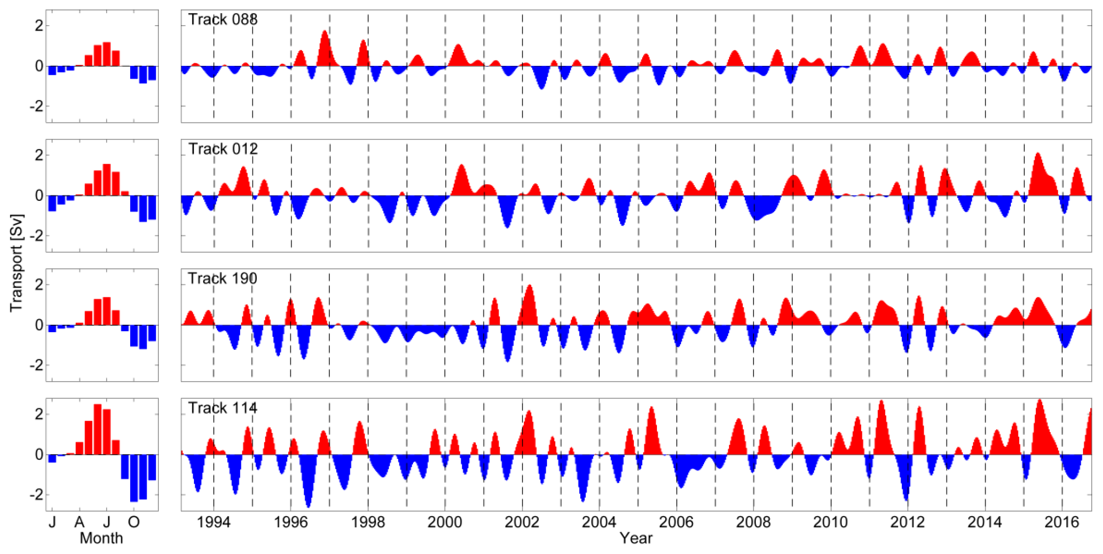
Seasonal cycles of along-shelf volume transport anomalies through four ground tracks show similar patterns (Figure 7 left). The transports are northeastward (positive values) from mid-spring to summer with maximum values in June or July and southwestward (negative values) from mid-autumn to winter with maximum values in October or November. Our results are consistent with the basin scale circulation [34]: cyclonic in the winter and anticyclonic in the summer, which is driven by the northeasterly and the southwesterly wind in the NSCS, respectively.
Interannual variabilities in along-shelf volume transport anomalies at ground track 088 has smaller amplitudes than the other three tracks, which is presumably due to complex bathymetry near the Taiwan Bank. Along-shelf volume transport anomalies from the years of 1998 and 1999 are almost southwestward in all ground tracks (Figure 7 right). This may indicate the influence of El Niño and needs further investigation.
4.1.2. Cross-Shelf Volume Transports
Cross-shelf volume transports are estimated based on the convergence and divergence of along-shelf volume transport anomalies in each control volume (CV), with the assumption that the long-term mean along-shelf volume transports at each cross-sections are identical. Control volumes are defined based on the boundaries of the coastline, the 200 m isobath, and two adjacent ground tracks. For example, the east control volume is the area between track 088 and track 012, named CV088012. In this study, we focus on three control volumes from east to west, which can represent the area near Dongsha Islands (CV088012), off the Pearl River Estuary (CV012190), and to the northeast of Hainan Island (CV190114). If the inflow volume from the west ground track is greater (or smaller) than the outflow volume from the east ground track, there is a net offshore (or onshore) transport in the control volume, assuming that there is no flow through the coastline. Similar assumptions and estimations have been successfully applied in calculating the cross-shelf volume transport in the South Atlantic Bight and are in agreement with numerical model results and ADCP estimations [23]. This theory has a simple assumption, for example, convergence in the surface layer is at least partially compensated by divergence in the bottom layer, especially during strong stratification periods when the coupling effects are smaller between the surface and bottom flow. If the cross-shelf volume transport in the surface layer is compensated by opposite transport in the bottom layer, the cross-shelf volume transport may also occur even though there is no exchange across the two neighboring transects. Detailed discussions about the limitations of the calculation and possible implications of these assumptions can be found in Reference [23].
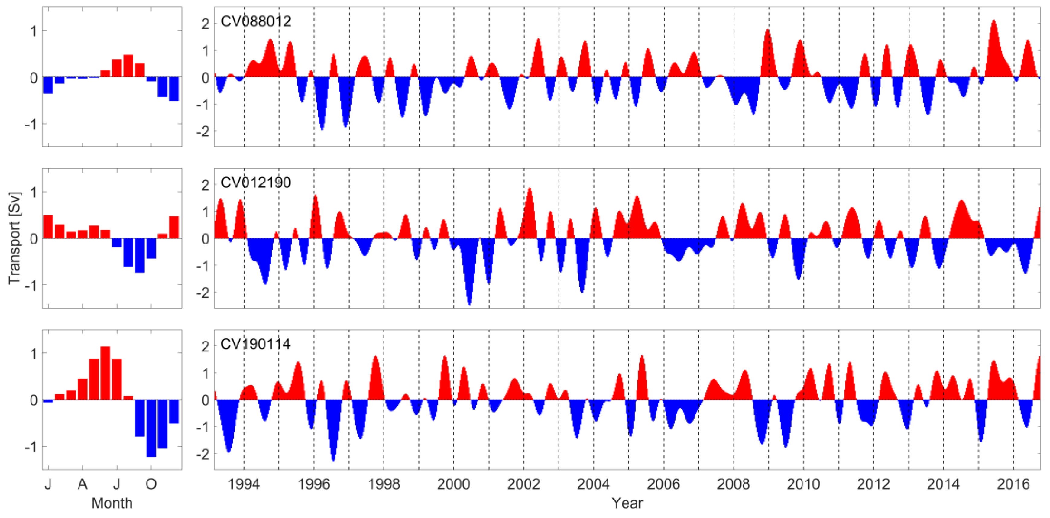
Figure 8 shows that the seasonal cycles of cross-shelf volume transports in the NSCS are in the offshore direction in early summer and in the onshore direction in mid-autumn. The interannual variations of the cross-shelf volume transport show their response to El Niño. The correlation coefficient (95% CL) between the cross-shelf volume transport near Dongsha Islands (CV088012) and Niño 3.4 index is 0.331 (0.285). Qu, et al. [5] also revealed that the Luzon Strait transport seems to be a key process in conveying the impact of ENSO (El Niño and Southern Oscillation) into the SCS based on results from numerical ocean models.
Cross-shelf volume transport off the Pearl River Estuary is further compared with the volume transport estimated from moored ADCP. The estimated cross-shelf volume transport is simply integrated into the ADCP velocity with the depth and then multiplied with the width between track 012 and track 190. It is important to illustrate that such a comparison is very challenging as we only use the cross-shelf velocity from one mooring ADCP to represent the average velocity through the 200 m isobath. As the magnitude of cross-shelf velocities is small and highly variable along the 200 m isobath, cross-shelf velocities from one moored ADCP cannot provide a robust estimation of the cross-shelf volume transport. However, this simple calculation allows us to roughly validate cross-shelf volume transports based on altimeter-derived velocities if we assume the main flow in this region is approximately along the continental shelf [23].
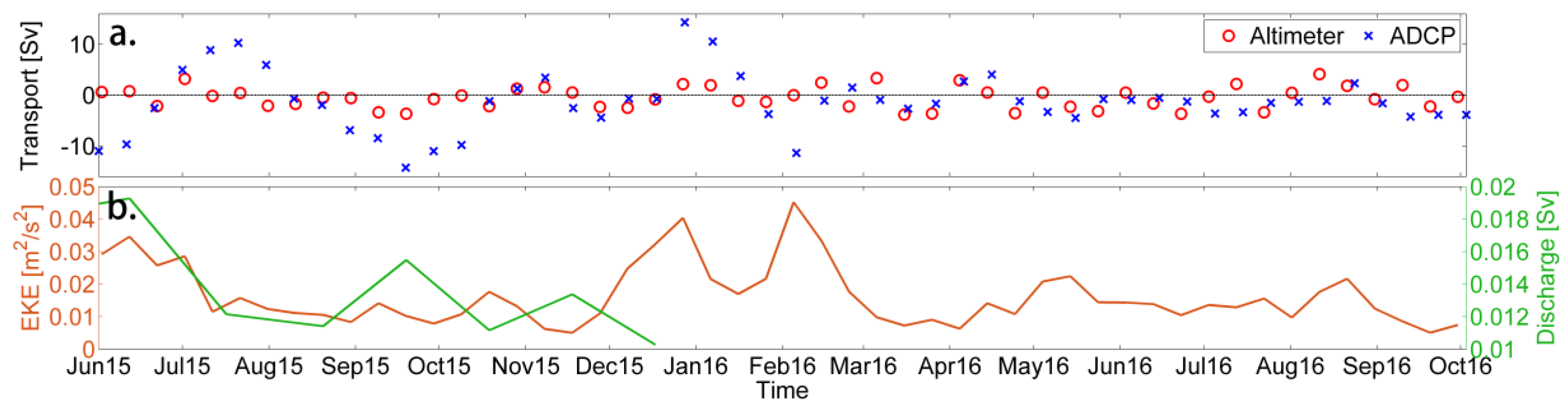
Altimeter-derived and ADCP-estimated cross-shelf volume transports have similar values, especially when eddy kinetic energy (EKE) and Pearl River discharge are low (Figure 9). Comparisons show significant differences between the two transports when EKE is high or Pearl River discharge is large, indicating that mesoscale processes (e.g., mesoscale eddies, internal waves) have some impact on the cross-shelf volume transport. The vertical profile of ADCP-measured velocity below 37 m also shows little variation vertically at the period when EKE and Pearl River discharge are low (e.g., August 2015 in Figure 6a) and stronger variation when EKE is high (e.g., February 2016 in Figure 6b). Cheng, et al. [15] found that the current velocity observed from moored ADCP near Dongsha Islands shows dominated energy in the barotropic mode most of the time; however, they found enhanced energy in the first baroclinic mode during the occurrence of eddies due to an enhanced vertical velocity shear. Moreover, freshwater discharge increases the stratification in the region, which may also introduce a baroclinic effect [35]. In the control volume calculation, the altimeter calculates the bulk transport, while ADCP just measure velocities at a single point. Enhanced mesoscale processes or stratification may further increase the distinction between the bulk estimation and the single point measurement. Therefore, the results suggest that our theory of computing cross-shelf volume transport through convergence and divergence in the control volume is valid when EKE and discharge are relatively low, i.e., when the barotropic effect dominates.
4.2. External Forces Controlling Cross-Shelf Volume Transports in the NSCS
In this section, we examine the relationship between the cross-shelf volume transport and potential external forces by using the 24-year time series of cross-shelf volume transports estimated in the previous section. We focus on four potential mechanisms in driving cross-shelf volume transports in the NSCS based on previous studies: winds [7,34], Kuroshio intrusion [1,6,12], Pearl River discharge [14], and El Niño effects [7,36,37]. We further use a multiple linear regression method to reconstruct cross-shelf volume transports using the mechanisms that show significant influences on the transport.
The spatial mean MADT time series over 115–120° E and 15–20° N is a reliable index to evaluate Kuroshio intrusion through the Luzon Strait [38]. The spatial mean of cross-shelf wind over areas that are bounded with two neighboring altimeter ground tracks, coastline, and 200 m isobath is used as the wind factor. Pearl River discharge is represented by the sum of three hydrological stations (GY, SJ, and BL). Cross-shelf volume transports are reconstructed as the sum of annual and semi-annual harmonics, cross-shelf wind stress, Kuroshio intrusion, Pearl River discharge, and El Niño. Those possible factors are cross-related, especially on the time scale of seasonal cycles that can reduce the number of observations [39], but factors used for multiple linear regression should be independent to each other. Therefore, as in Reference [39], the four factors (wind stress, Kurohio, discharge, and El Niño) are subtracted their corresponding seasonal cycles, then the seasonal cycles are combined to reconstruct cross-shelf volume transports in the NSCS. The reconstructed cross-shelf volume transports in the NSCS are able to capture the basic trends and most of the extremums during 2002 and 2015 (Figure 10). Detailed information regarding correlation coefficients and significant forces are shown in Table 2.
Correlation coefficients (95% CL) between reconstructed and measured cross-shelf volume transports are 0.461 (0.263), 0.372 (0.215) and 0.619 (0.268) for full time series near Dongsha Islands, off Pearl River Estuary and to the northeast of Hainan Island, respectively. If we only consider the low-frequency component, the correlations (95% CL) are 0.633 (0.263), 0.519 (0.263) and 0.839 (0.268) in corresponding areas. Our analysis indicates that the seasonal cycle is the major factor of cross-shelf volume transport, which accounts for 44.7%, 46.9% and 64.1% near Dongsha Islands, off Pearl River Estuary and to the northeast of Hainan Island in controlling the fate of cross-shelf volume transports in the NSCS. Guo, et al. [7] found that the first three leading EOF modes of SLA (accounting for 57% of the total variance) exhibited important seasonal features and showed remarkable characteristics in different seasons. Combining altimeter data and ocean models, Qu, et al. [40] suggested that semiannual signals are important in the upper layer circulation in western tropical Pacific Ocean. Our results also show high correlations between wind stress and seasonal cycles near Dongsha Islands and to the northeast of Hainan Island, indicating wind might be the primary mechanism in driving the seasonal cycles of cross-shelf volume transport. Unfortunately, with the present data we cannot confirm this hypothesis and it would need future studies combining numerical models.
The cross-shelf volume transport in the NSCS also shows its response to local wind and El Niño. Chen, et al. [11] found that the variation of the upper-layer circulation structure has high seasonal variation and is mostly dominated by the monsoon in the SCS. Results from ocean models or satellite altimetry showed that ENSO has impacts on the SCS circulation [5,7,36,37].
Additionally, Kuroshio intrusion and Pearl River discharge are important parameters in influencing cross-shelf volume transport off the Pearl River Estuary. By using the Princeton Ocean Model (POM), Xue, et al. [6] exhibited that Kuroshio intrusion often forms an anticyclonic current loop near the western Luzon Strait and the westward branch becomes the SCS Branch of Kuroshio intrusion on the NSCS slope. Chen and Chen [41] showed a highly spatial and interannual variability in biological production in the NSCS shelf region, with a relatively high production in summer due to Pearl River discharge; it being oligotrophic during winter. This presumably indicates the impact of freshwater discharge on the cross-shelf volume transport in the region near the Pearl River Estuary.
5. Conclusions
Satellite altimetry data from March 1993 to September 2016 were used to investigate circulation in the NSCS. Geostrophic velocity anomalies were calculated using the SLA at each location along the altimeter ground tracks. Adding the Ekman current to the geostrophic current does not significantly increase the correlation coefficients between altimeter-derived and ADCP-estimated velocity anomalies at 37 m, which may due to the fact that the Ekman current has important effects at the surface but its influence decreases dramatically in lower layers as the Ekman velocity descends exponentially with water depth. As geostrophic velocities are mean values in the near-surface layer, along-shelf volume transport anomalies were calculated as the integration along the altimeter ground tracks until the 200 m isobath by ignoring the vertical structure of the coastal current. There are northeastward transports from mid-spring to summer with peaks in June or July and southwestward transports from mid-autumn to winter with peaks in October or November; this is consistent with basin scale circulation in the NSCS. Cross-shelf volume transports were then calculated based on the convergence or divergence between neighboring along-shelf (cross-track) volume transport anomalies with the assumption that long-term mean along-shelf volume transports at each cross-sections are identical. Our results show that the cross-shelf volume transport is onshore in mid-autumn and offshore in early summer in the NSCS. The comparison between altimeter-derived and ADCP-estimated cross-shelf volume transport is at the same order of magnitude. Two time series are especially consistent when the region has relatively low mesoscale activities and a low Pearl River discharge.
In order to investigate the potential mechanisms controlling cross-shelf volume transports in the NSCS, multiple linear regressions are used to reconstruct cross-shelf volume transports based on annual and semi-annual harmonics, El Niño, cross-shelf wind, Kuroshio intrusion, and Pearl River discharge. Our results show that reconstructed cross-shelf volume transports can capture the overall tendency and most of the extremums in the NSCS. The seasonal cycle is the major factor controlling the cross-shelf volume transports in the NSCS, while El Niño and wind have secondary effects.
Acknowledgements
The authors would like to thank two anonymous reviewers for their thoughtful comments and suggestions, which resulted in a substantially improved manuscript. The authors also thank CTOH (http://ctoh.legos.obs-mip.fr), RSS (http://www.remss.com), AVISO (https://www.aviso.altimetry.fr), UHSLC (http://uhslc.soest.hawaii.edu) and MWR (http://www.mwr.gov.cn) for providing coastal sea level anomaly, CCMP wind, maps of absolute dynamic topography and UV maps of geostrophic velocity anomalies, tide gauge, and Pearl River discharge data, respectively.
Funding
This study is supported by National Basic Research Program of China (No. 2014CB441501), National Natural Science Foundation of China (No. 41506101 and No. 41406021). Support by SOED Young Ocean Star Scholar (QNHX1611) to Y.Y. and project of State Key Laboratory of Satellite Ocean Environment Dynamics (SOED), Second Institute of Oceanography (SIO) (Grant No. SOEDZZ1704) to D.X. is also acknowledge.
Author Contributions
All of the authors have contributed to this paper. Jin Liu analyzed the data and wrote the manuscript, Juanjuan Dai wrote the manuscript, Dongfeng Xu and Jun Wang obtained and analyzed the moored ADCP data, Yeping Yuan is the corresponding author who designed the idea and revised the paper.
Conflicts of Interest
The authors declare no conflict of interest. The funding sponsors had no role in the design of the study; in the collection, analysis, or interpretation of data; in the writing of the manuscript, and in the decision to publish the results.
References
- Nan, F.; Xue, H.; Chai, F.; Shi, L.; Shi, M.; Guo, P. Identification of different types of Kuroshio intrusion into the South China Sea. Ocean Dyn. 2011, 61, 1291–1304. [Google Scholar] [CrossRef]
- Su, J. Overview of the South China Sea circulation and its influence on the coastal physical oceanography outside the Pearl River Estuary. Cont. Shelf Res. 2004, 24, 1745–1760. [Google Scholar] [CrossRef]
- Zhang, J.; Yu, Z.; Wang, J.; Ren, J.; Chen, H.; Xiong, H.; Dong, L.; Xu, W. The subtropical Zhujiang (Pearl River) estuary: Nutrient, trace species and their relationship to photosynthesis. Estuar. Coast. Shelf Sci. 1999, 49, 385–400. [Google Scholar] [CrossRef]
- Qu, T. Upper-layer circulation in the South China Sea. J. Phys. Oceanogr. 2000, 30, 1450–1460. [Google Scholar] [CrossRef]
- Qu, T.; Kim, Y.Y.; Yaremchuk, M.; Tozuka, T.; Ishida, A.; Yamagata, T. Can Luzon Strait transport play a role in conveying the impact of ENSO to the South China Sea? J. Clim. 2004, 17, 3644–3657. [Google Scholar] [CrossRef]
- Xue, H.; Chai, F.; Pettigrew, N.; Xu, D.; Shi, M.; Xu, J. Kuroshio intrusion and the circulation in the South China Sea. J. Geophys. Res. Oceans 2004, 109. [Google Scholar] [CrossRef]
- Guo, J.; Fang, W.; Fang, G.; Chen, H. Variability of surface circulation in the South China Sea from satellite altimeter data. Chin. Sci. Bull. 2006, 51, 1–8. [Google Scholar] [CrossRef]
- Fang, G.; Wang, Y.; Wei, Z.; Fang, Y.; Qiao, F.; Hu, X. Interocean circulation and heat and freshwater budgets of the South China Sea based on a numerical model. Dyn. Atmos. Oceans 2009, 47, 55–72. [Google Scholar] [CrossRef]
- Wang, Q.; Cui, H.; Zhang, S.; Hu, D. Water transports through the four main straits around the South China Sea. Chin. J. Oceanol. Limnol. 2009, 27, 229. [Google Scholar] [CrossRef]
- Fang, G.; Susanto, R.D.; Wirasantosa, S.; Qiao, F.; Supangat, A.; Fan, B.; Wei, Z.; Sulistiyo, B.; Li, S. Volume, heat, and freshwater transports from the South China Sea to Indonesian seas in the boreal winter of 2007–2008. J. Geophys. Res. Oceans 2010, 115. [Google Scholar] [CrossRef]
- Chen, C.; Zhu, J.; Wang, H.; Huang, X. Studies of upper layer circulations of the South China Sea from Satellite altimeter observation. In IOP Conference Series: Earth and Environmental Science; IOP Publishing: Bristol, UK, 2014; p. 012118. [Google Scholar]
- Nan, F.; Xue, H.; Yu, F. Kuroshio intrusion into the South China Sea: A review. Prog. Oceanogr. 2014, 137, 314–333. [Google Scholar] [CrossRef]
- Zhang, S.; Lu, X.X.; Higgitt, D.L.; Chen, C.-T.A.; Han, J.; Sun, H. Recent changes of water discharge and sediment load in the Zhujiang (Pearl River) Basin, China. Glob. Planet. Chang. 2008, 60, 365–380. [Google Scholar] [CrossRef]
- He, X.; Xu, D.; Bai, Y.; Pan, D.; Chen, C.-T.A.; Chen, X.; Gong, F. Eddy-entrained Pearl River plume into the oligotrophic basin of the South China Sea. Cont. Shelf Res. 2016, 124, 117–124. [Google Scholar] [CrossRef]
- Cheng, L.; Zhang, Z.; Zhao, W.; Tian, J. Temporal variability of the current in the northeastern South China Sea revealed by 2.5-year-long moored observations. J. Oceanogr. 2015, 71, 361–372. [Google Scholar] [CrossRef]
- Zhu, X.; Zhao, R.; Guo, X.; Long, Y.; Ma, Y.; Fan, X. A long-term volume transport time series estimated by combining in situ observation and satellite altimeter data in the northern South China Sea. J. Oceanogr. 2015, 71, 663–673. [Google Scholar] [CrossRef]
- Han, G. TOPEX/Poseidon-Jason comparison and combination off Nova Scotia. Mar. Geodesy 2004, 27, 577–595. [Google Scholar] [CrossRef]
- Vignudelli, S.; Cipollini, P.; Roblou, L.; Lyard, F.; Gasparini, G.; Manzella, G.; Astraldi, M. Improved satellite altimetry in coastal systems: Case study of the Corsica Channel (Mediterranean Sea). Geophys. Res. Lett. 2005, 32. [Google Scholar] [CrossRef]
- Han, G. Satellite observations of seasonal and interannual changes of sea level and currents over the Scotian Slope. J. Phys. Oceanogr. 2007, 37, 1051–1065. [Google Scholar] [CrossRef]
- Saraceno, M.; Strub, P.T.; Kosro, P.M. Estimates of sea surface height and near-surface alongshore coastal currents from combinations of altimeters and tide gauges. J. Geophys. Res. Oceans 2008, 113. [Google Scholar] [CrossRef]
- Liu, Y.; Weisberg, R.H.; Vignudelli, S.; Roblou, L.; Merz, C.R. Comparison of the X-TRACK altimetry estimated currents with moored ADCP and HF radar observations on the West Florida Shelf. Adv. Space Res. 2012, 50, 1085–1098. [Google Scholar] [CrossRef]
- Strub, P.T.; James, C.; Combes, V.; Matano, R.P.; Piola, A.R.; Palma, E.D.; Saraceno, M.; Guerrero, R.A.; Fenco, H.; Ruiz-Etcheverry, L.A. Altimeter-derived seasonal circulation on the southwest Atlantic shelf: 27°–43° S. J. Geophys. Res. Oceans 2015, 120, 3391–3418. [Google Scholar] [CrossRef] [PubMed]
- Yuan, Y.; Castelao, R.M.; He, R. Variability in along-shelf and cross-shelf circulation in the South Atlantic Bight. Cont. Shelf Res. 2017, 134, 52–62. [Google Scholar] [CrossRef]
- Strub, P.T.; Chereskin, T.K.; Niiler, P.P.; James, C.; Levine, M.D. Altimeter-derived variability of surface velocities in the California Current System: 1. Evaluation of TOPEX altimeter velocity resolution. J. Geophys. Res. Oceans 1997, 102. [Google Scholar] [CrossRef]
- Morrow, R.; Coleman, R.; Church, J.; Chelton, D. Surface Eddy Momentum Flux and Velocity Variances in the Southern Ocean from Geosat Altimetry. J. Phys. Oceanogr. 1994, 24, 2050–2071. [Google Scholar] [CrossRef]
- Atlas, R.; Hoffman, R.N.; Ardizzone, J.; Leidner, S.M.; Jusem, J.C.; Smith, D.K.; Gombos, D. A Cross-calibrated, Multiplatform Ocean Surface Wind Velocity Product for Meteorological and Oceanographic Applications. Bull. Am. Meteorol. Soc. 2011, 92, 157–174. [Google Scholar] [CrossRef]
- Large, W.; Pond, S. Open ocean momentum flux measurements in moderate to strong winds. J. Phys. Oceanogr. 1981, 11, 324–336. [Google Scholar] [CrossRef]
- Austin, J.A.; Barth, J.A. Variation in the position of the upwelling front on the Oregon shelf. J. Geophys. Res. Oceans 2002, 107. [Google Scholar] [CrossRef]
- Ekman, V.W. On the Influence of the Earth’s Rotation on Ocean-Currents. Available online: https://jscholarship.library.jhu.edu/handle/1774.2/33989 (accessed on 20 April 2018).
- McPhee, M. Air-Ice-Ocean Interaction: Turbulent Ocean Boundary Layer Exchange Processes; Springer Science & Business Media: Berlin, Germnay, 2008. [Google Scholar]
- Stewart, R.H. Introduction to Physical Oceanography; Texas A & M University: College Station, TX, USA, 2008. [Google Scholar]
- Keister, J.E.; Strub, P.T. Spatial and interannual variability in mesoscale circulation in the northern California Current System. J. Geophys. Res. Oceans 2008, 113. [Google Scholar] [CrossRef]
- Walker, A.E.; Wilkin, J.L. Optimal averaging of NOAA/NASA Pathfinder satellite sea surface temperature data. J. Geophys. Res. Oceans 1998, 103, 12869–12883. [Google Scholar] [CrossRef]
- Fang, W.; Guo, J.; Shi, P.; Mao, Q. Low frequency variability of South China Sea surface circulation from 11 years of satellite altimeter data. Geophys. Res. Lett. 2006, 33. [Google Scholar] [CrossRef]
- Robinson, A.R.; Brink, K.H. The Global Coastal Ocean: Multiscale Interdisciplinary Processes; Harvard University Press: Cambridge, MA, USA, 2005; Volume 11. [Google Scholar]
- Xie, S.; Xie, Q.; Wang, D.; Liu, W.T. Summer upwelling in the South China Sea and its role in regional climate variations. J. Geophys. Res. Oceans 2003, 108. [Google Scholar] [CrossRef]
- Wang, Y.; Fang, G.; Wei, Z.; Qiao, F.; Chen, H. Interannual variation of the South China Sea circulation and its relation to El Niño, as seen from a variable grid global ocean model. J. Geophys. Res. Oceans 2006, 111. [Google Scholar] [CrossRef]
- Wu, C.-R. Interannual modulation of the Pacific Decadal Oscillation (PDO) on the low-latitude western North Pacific. Prog. Oceanogr. 2013, 110, 49–58. [Google Scholar] [CrossRef]
- Chelton, D.B.; Davis, R.E. Monthly Mean Sea-Level Variability Along the West Coast of North America. J. Phys. Oceanogr. 1982, 12, 757–784. [Google Scholar] [CrossRef]
- Qu, T.; Gan, J.; Akio, I.; Yuji, K.; Tomoki, T. Semiannual variation in the western tropical Pacific Ocean. Geophys. Res. Lett. 2008, 35, 134–143. [Google Scholar] [CrossRef]
- Chen, Y.-L.L.; Chen, H.-Y. Seasonal dynamics of primary and new production in the northern South China Sea: The significance of river discharge and nutrient advection. Deep Sea Res. Part I 2006, 53, 971–986. [Google Scholar] [CrossRef]
Figure 1.
(a) Map of the South China Sea (SCS). TS: the Taiwan Strait, LS: the Luzon Strait, MS: the Mindoro Strait, BS: the Balabac Strait, KS: the Karimata Strait; (b) Map of the northern SCS (NSCS) and altimeter ground tracks (colored dots). The percentage of valid data along the four ground tracks are shown in different colors and the track numbers are shown in red. The 50, 200, and 2000 m isobaths are shown in light to dark gray. The location of moored acoustic Doppler current profilers (ADCP) is indicated with the green pentagram. The nearest point with ADCP along track 190 used in the validation is shown as a green triangle. The location of tide gauges (TG) are shown as blue squares. SW: Shanwei, HK: Hong Kong, ZP: Zhapo. The three hydrologic stations are shown as red diamonds. GY: Gaoyao, SJ: Shijiao, BL: Boluo.

Figure 2.
Comparisons of sea level anomalies (SLA) between TG data and the nearest valid along-track altimeter data. Correlation coefficients (95% confidence level (CL)) between two time series and root mean square differences (RMSDs) are shown in the upper left corner in each panel.
Figure 2.
Comparisons of sea level anomalies (SLA) between TG data and the nearest valid along-track altimeter data. Correlation coefficients (95% confidence level (CL)) between two time series and root mean square differences (RMSDs) are shown in the upper left corner in each panel.

Figure 3.
Seasonal cycles (left column) and interannual variabilities (right column) in SLA along four ground tracks within 200 m isobath. Positive or negative values represent above or below the mean sea level, respectively. Track numbers are shown in the upper left corner of left column panels.
Figure 3.
Seasonal cycles (left column) and interannual variabilities (right column) in SLA along four ground tracks within 200 m isobath. Positive or negative values represent above or below the mean sea level, respectively. Track numbers are shown in the upper left corner of left column panels.

Figure 4.
Seasonal cycles (left column) and interannual variabilities (right column) in geostrophic velocity anomalies across four ground tracks. Positive or negative values represent flow towards the northeast or southwest directions, respectively. Track numbers are shown in the upper left corner of left column panels.

Figure 5.
(a) Altimeter-derived and ADCP-measured monthly mean along-shelf velocity anomalies; (b) altimeter-derived and ADCP-measured full along-shelf velocity anomalies time series. The correlation coefficient and RMSD are shown in the upper left corner of the panel.
Figure 5.
(a) Altimeter-derived and ADCP-measured monthly mean along-shelf velocity anomalies; (b) altimeter-derived and ADCP-measured full along-shelf velocity anomalies time series. The correlation coefficient and RMSD are shown in the upper left corner of the panel.

Figure 6.
(a) The vertical profile of velocity anomalies from moored ADCP in August 2015; (b) the vertical profile of velocity anomalies from moored ADCP in February 2016.
Figure 6.
(a) The vertical profile of velocity anomalies from moored ADCP in August 2015; (b) the vertical profile of velocity anomalies from moored ADCP in February 2016.

Figure 7.
Seasonal cycles (left column) and interannual variabilities (right column) of along-shelf volume transport anomalies across the four ground tracks. Positive (red) or negative (blue) values represent northeastward or southwestward transports, respectively. Track numbers are shown in the upper left corner of right column panels.

Figure 8.
Seasonal cycles (left column) and interannual variabilities (right column) of cross-shelf volume transports across 200 m isobath near Dongsha Islands (CV088012), off the Pearl River Estuary (CV012190) and to the northeast of Hainan Island (CV190114). Positive and negative values represent offshore and onshore transports, respectively. Numbers of each control volume are shown in the upper left corner of right column panels.

Figure 9.
(a) Altimeter-derived and ADCP-estimated cross-shelf volume transport time series off the Pearl River Estuary during June 2015 and October 2016; (b) averaged eddy kinetic energy (EKE) bounded by two ground tracks and 200 m isobath and Pear River discharge time series during the same period.

Figure 10.
Comparisons between altimeter-derived and reconstructed full cross-shelf volume transports near Dongsha Islands (CV088012), off the Pearl River Estuary (CV012190), and to the northeast of Hainan Island (CV190114). Numbers of control volume, correlation coefficients (95% CL), and RMSDs are shown in the upper left corner of each panel.


Table 1.
Data information in this study.
| Name of Location | Instrument | Longitude (° E) | Latitude (° N) | Time Coverage |
|---|---|---|---|---|
| SW | TG | 115.35 | 22.75 | Mar 1993-Dec 1997 |
| HK | TG | 114.22 | 22.60 | Mar 1993-Jul 2015 |
| ZP | TG | 111.83 | 21.58 | Mar 1993-Dec 1997 |
| — | ADCP | 115.00 | 19.50 | May 2015-Sep 2016 |
| GY | HS | 112.44 | 23.05 | Jan 2002-Dec 2015 |
| SJ | HS | 112.97 | 23.53 | Jan 2002-Dec 2015 |
| BL | HS | 114.28 | 23.18 | Jan 2002-Dec 2015 |
SW: Shanwei, HK: Hong Kong, ZP: Zhapo, GY: Gaoyao, SJ: Shijiao, BL: Boluo, TG: tide gauge, ADCP: acoustic Doppler current profiler, HS: hydrological station.
Table 2.
Results of reconstructed cross-shelf volume transports in the NSCS.
| Control Volume | Correlation (95% CL) | Seasonal Cycle * | Wind * | Kuroshio Intrusion * | Pearl River Discharge * | El Niño* |
|---|---|---|---|---|---|---|
| CV088012 | 0.461 (0.263) | 0.319 (44.7%) | 0.161 (22.6%) | — | — | 0.233 (32.7%) |
| CV012190 | 0.372 (0.215) | 0.319 (46.9%) | 0.091 (13.4%) | 0.085 (12.5%) | 0.050 (7.4%) | 0.135 (19.8%) |
| CV190114 | 0.619 (0.268) | 0.563 (64.1%) | 0.107 (12.2%) | — | — | 0.208 (23.7%) |
CV088012: near Dongsha Islands, CV012190: off Pearl River Estuary, CV190114: to the northeast of Hainan Island. * Multiple linear regression coefficients and corresponding proportions (in brackets) of elements are below the factors. — represents the factor does not have significantly contribution in multiple linear regression in this control volume.
© 2018 by the authors. Licensee MDPI, Basel, Switzerland. This article is an open access article distributed under the terms and conditions of the Creative Commons Attribution (CC BY) license (http://creativecommons.org/licenses/by/4.0/).
Share and Cite
MDPI and ACS Style
Liu, J.; Dai, J.; Xu, D.; Wang, J.; Yuan, Y. Seasonal and Interannual Variability in Coastal Circulations in the Northern South China Sea. Water 2018, 10, 520. https://doi.org/10.3390/w10040520
AMA Style
Liu J, Dai J, Xu D, Wang J, Yuan Y. Seasonal and Interannual Variability in Coastal Circulations in the Northern South China Sea. Water. 2018; 10(4):520. https://doi.org/10.3390/w10040520
Chicago/Turabian StyleLiu, Jin, Juanjuan Dai, Dongfeng Xu, Jun Wang, and Yeping Yuan. 2018. "Seasonal and Interannual Variability in Coastal Circulations in the Northern South China Sea" Water 10, no. 4: 520. https://doi.org/10.3390/w10040520
Note that from the first issue of 2016, this journal uses article numbers instead of page numbers. See further details here.