The Upwelling Water Flux Feeding Springs: Hydrogeological and Hydraulic Features


Department of Science and Technology, University of Sannio, 82100 Benevento, Italy
*
Author to whom correspondence should be addressed.
Water 2018, 10(4), 501; https://doi.org/10.3390/w10040501
Submission received: 8 March 2018
/
Revised: 11 April 2018
/
Accepted: 13 April 2018
/
Published: 18 April 2018
(This article belongs to the Special Issue Water Resources Investigation: Geologic Controls on Groundwater Flow)
Abstract
:The upwelling groundwater flux has been investigated by deep piezometers in a spring area characterized by alluvial deposits covering a karst substratum in Southern Italy. The piezometers are of varying depth located in a flat area. They have been monitored for a long period (about 40 years), and when measured, a good relationship between spring discharge and hydraulic head was observed. The local upwelling groundwater flux has been deducted by the increasing of the hydraulic head in depth, which allows the estimation of ascendant hydraulic gradient and groundwater velocity during the dry and wet seasons. A specific analytical solution has been used to estimate the zone involved by the ascendant flow, and could also be used in other spring areas. Some physical and chemical characteristics of spring water have been collected, including the radon (222Rn) activity, to support the phenomenon of the ascendant flux. The man geological and hydrogeological features leading to ascendant flux in karst environments is also discussed for some areas of Southern Italy, where many springs are affected.
1. Introduction
Springs are among the essential features of the hydrological cycle, as their main characteristics such as discharge, temperature and chemistry can be measured, giving fundamental knowledge of groundwater flow.
The location of springs depend on the local topographic and hydrogeological features, and most of them originate along geological contacts, faults and ground depressions [1,2].
Following the model of regional groundwater flow [3,4,5] the discharge areas are located in depressed zones which increases the river discharge by diffused recharge or by springs. In these areas, the vertical component of the flux can be higher than the horizontal one, and the water flux develops in a typical ascendant path.
The ascendant flux occurring in the discharge area can lead to the start-up of a river, especially in the karst mountain areas, where powerful springs are fed by a wide catchment which supports high discharge for the entire hydrological year. In other cases, rivers increase their discharge when crossing zones are characterized by ascendant groundwater flow [6].
Karst aquifers, characterized by high transmissivity and generally by capacity to store large volumes of groundwater [7,8], can allow deep water circulation which leads to the start of the ascendant flux in the discharge zone.
Although, spring discharge measurements can be easily or directly measured directly at the source or along a river, the connected ascendant flux is not easily detected, because it needs the knowledge of the vertical hydraulic gradient to be distinguished from the most common horizontal flow. Without the knowledge of the actual path of the spring flow, some hydrologic processes may be poorly understood which could lead to inappropriate water management, as the delimitation of the protection zones of springs.
In this study, we focused on the ascendant flux feeding karst springs, measuring the vertical hydraulic gradient by monitoring deep piezometers. The spring area is located near the village of Serino, along the Sabato River, Southern Italy, where long monitoring data are available for spring discharge and piezometers.
A method used to estimate the wideness of the zone involved in the ascendant flux has been provided, which can be used for other similar spring areas, characterized by ascendant flux. The estimation is an important tool for delineating the protection zone of springs characterized by ascendant flux.
To support this hydraulic phenomenon, deducted from the analysis of hydraulic head monitored into several piezometers and located in the discharge area, specific geochemical measurements have been carried out by monitoring the radon (222Rn) activity of spring water.
In general, we found that the ascendant flux is a topic not regularly discussed in literature. The aim of this study is to provide a detailed case history, which applies to other areas of Southern Italy, and perhaps elsewhere.
2. Materials and Methods
2.1. Ascendant Hydraulic Gradient and Wideness of Influenced Zone
The ascendant flow has been investigated by deep piezometers, where the ascendant hydraulic gradient has been estimated from measurements of the hydraulic head.
In the discharge area where springs are located, we assume that the piezometer depth can have a strong control over the hydraulic head measured due to non-hydrostatic conditions, particularly, under descendant or ascendant groundwater flux [9].
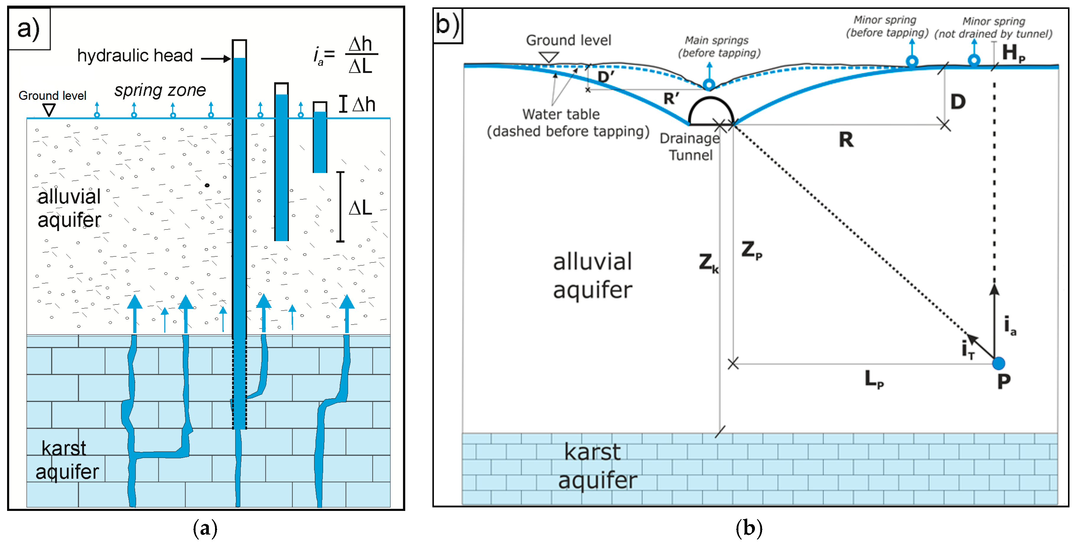
Figure 1a shows the estimation of the vertical hydraulic gradient by the hydraulic head measurements in wells; here the difference in the hydraulic head measured in two close boreholes is caused by the vertical (ascendant) flux. This estimation is based on the assumption that no horizontal component of the flow occurs, and the hydraulic head is lost during the ascendant path of the flow. The estimated ascendant hydraulic gradient has been considered as an hydraulic model, where analytical solutions define some geometrical features of the phenomenon, particularly the wideness of the zone involved by the ascendant flux feeding springs or drainage systems.
In literature, analytical solutions of discharge drained by deep drainage have been provided by Hooghoudt [10]. Later on, other authors [11,12] improved the analytical procedure of Hooghoudt’s method. In general, this model assumes steady drainage towards ditches (or tile drains) in homogenous soil underlain by an impervious layer; it applies the radial flow equation to the region near the drains and the ellipse equation to the region away from the drains to determine the water table drop (or head loss) in each region. The water table drops on each region were added to find the total drop. This method is a useful practice procedure for designing a drainage system, aimed at regulating the water table of an unconfined aquifer, under a constant steady-state recharge. However, in the Hooghoudt’s model, a prevalent horizontal flow through the porous media is induced by the drainage system, and no ascendant flux toward the drainage is considered; moreover, an impervious layer is fixed below the drainage system.
Other types of analytical solutions have been provided to calculate steady-state inflow into a circular tunnel [13,14,15,16] useful for the design of the tunnel’s drainage systems [17]. In these models, the discharge drained by the tunnel depends on some geometrical and hydraulic features, such as the depth of the tunnel, the groundwater level, the tunnel radius and the hydraulic conductivity of the aquifer. The transient conditions are not considered, as the aim is to obtain the groundwater inflow (volume of water for unit tunnel length) generated by the introduction of a tunnel in an initial hydrostatic system. The inflow converges into the tunnel (thus the flow is ascendant in the inverse zone of the tunnel), and the differences between inflows at the crown and invert decrease with increasing depth of the tunnel under the groundwater table. As these models assume initial hydrostatic conditions, they cannot take into account the ascendant groundwater flow condition.
To estimate the influenced zone of the aquifer by the drainage tunnel, a simple 2D model is provided under a non-hydrostatic initial condition, where an ascendant hydraulic gradient causes the upwelling flow. The aim is not to estimate the inflow or the discharge in steady-state conditions, which would need a more complex approach (which is beyond the scope of this work), but to analyze the role of ascendant hydraulic gradient on the wideness of zone involved by the ascendant flow, namely the influenced zone. This aspect plays a fundamental role in delimitating the protection zone of springs and their tapping systems.
To estimate the width of the influenced zone, with distance R from a drainage tunnel or from a spring, the analytical solution assumes: (i) constant hydraulic conductivity in all directions; (ii) high aquifer thickness to guarantee vertical flow lines below a specific depth from the drainage system or spring; (iii) each flow line follows the direction of “maximum slope”.
Under these assumptions, the drainage system induces a potential hydraulic gradient, iT, in each generic point P of the aquifer (Figure 1b); a generic flow line continues along its vertical ascendant path for iT < ia, and up to iT = ia. When the condition changes, iT > ia, the flow line diverges from the vertical and tends to reach the drainage system (or springs). From Figure 1b, the ascendant hydraulic gradient, ia, and potential hydraulic gradient, iT, are computed as:
where HP is the excess hydraulic head of the point P with respect to the undisturbed water table; D is the elevation difference between the undisturbed water table and drainage system; ZP is the depth of point P with respect to the drainage system; and LP is the distance of point P from the drainage system.
If equations are related to the spring outlet, then the parameters D, ZP and LP have to be replaced by D’, ZP’ and LP’ (Figure 1b).
2.2. Physical and Chemical Characteristics Measurements
Monthly temperature, electrical conductivity and radon (222Rn) activity measurements have been carried out in the spring water.
Temperature and electrical conductivity have been detected by multiparameter probe (Horiba mod.U50), immersing the sensor directly in the spring water outlet.
The measurements of 222Rn activity have been carried out in spring water; water samples were taken directly into the drainage tunnel of the spring tapping system, from the depth of about 0.5 m below the level of water surface, using 500 mL glass bottles. Completely filed bottles were tightly closed when still submerged to prevent the entry of air and the release of radon from it. The samples, immediately sealed by parafilms, were transported to the laboratory of Hydrogeology of the University of Sannio for radon activity measurements with a minimum delay from collection time (30’). The 222Rn activity was performed using AlphaGUARD radon detector (Genitron Instruments GmbH, Germany): a pulse-counting ionization chamber suitable for alpha spectroscopy. Water samples of 100 mL were placed in the appropriate system of glass vessels. Detected 222Rn activity levels were analyzed using the software Data EXPERT (by GENITRON Instruments).
The main interest of 222Rn activity in spring water is its possible connection with groundwater velocity and, consequently, its variation during the high or low flow conditions of springs.
3. Geological and Hydrogeological Setting
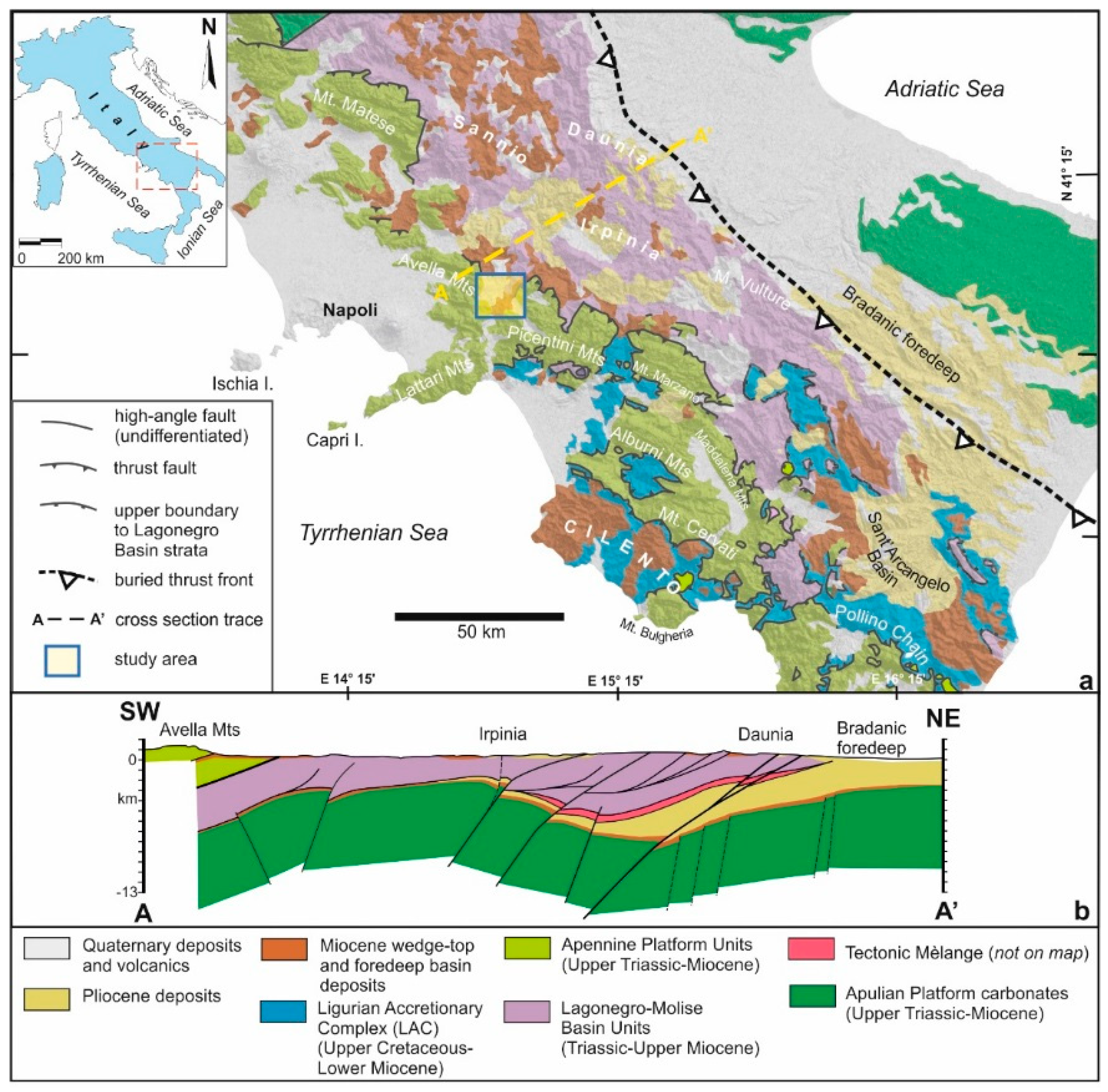
The study area is located in Southern Italy, inland of about 40 km from Naples, on the north-western boundary of the Picentini Mountains, including the high and middle valley of the Sabato River. Locally, there are several different geological formation outcrops, forming part of the Irpinia Apennine chain (Figure 2).
The outcropping sedimentary successions, as described in a recent geological map (ISPRA, 2017), are grouped into several stratigraphic or tectonic units: (i) Mesozoic platform carbonates of the Picentini Unit with a high permeability rate; (ii) Meso-Cenozoic deep-basin deposits of the Lagonegro Unit with a low permeability rate; (iii) upper Tortonian/lower Messinian wedge-top basin clastic sediments of the Castelvetere Fm. with a low permeability rate; (iv) deposits of Quaternary age with a medium-high permeability rate.
The tectonic record highlights several main sequences of events, from the carbonate platform involved in the wedge accretion and north/east-ward overthrust onto the Lagonegro basin deposits during the lower-middle Miocene [18] to extensional tectonic movements of Plio-Pleistocene, where the NW-SE left-lateral strike-slip main fault [19], crossing the Sabato River valley was generated. Subsequently, the extensional movements, especially the Tyrrhenian side of the chain, induced the creation of the Sabato River graben, filled by fluvio-lacustrine sediments.
These tectonic regimes induced a hydrogeological framework that has dislocated carbonate rocks in high morphological element (horst) and low morphological element (graben), creating a ground space between the recharge area and the discharge area.
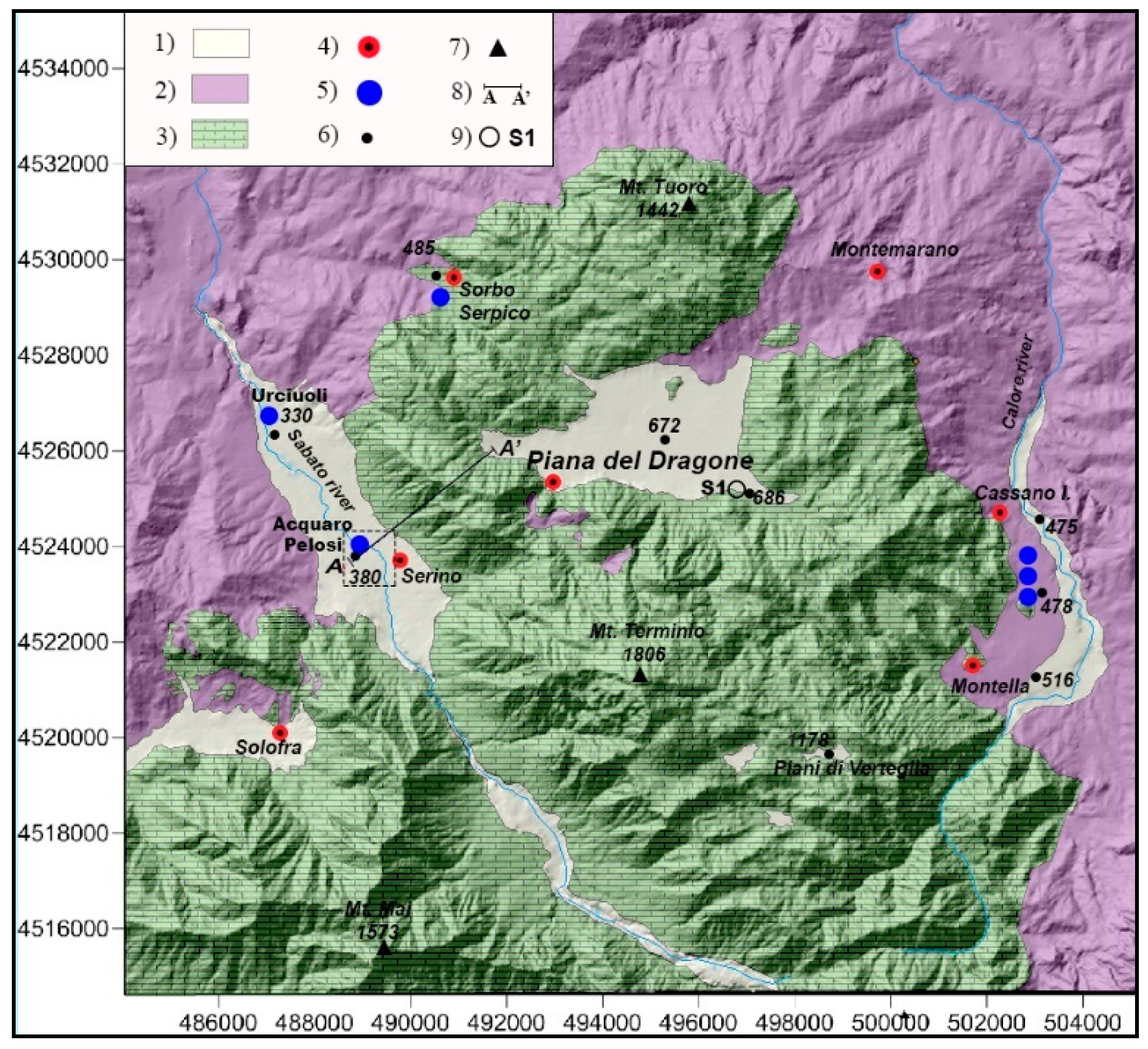
In this context, the Terminio-Tuoro massif constitutes a wide karst system, feeding several karst springs (Figure 3).
The entire karst area is estimated to be about 163 km2 and provides a total spring discharged water volume of 170.5 × 10⁶ m3/year [20]. It is arduous to define each spring catchment, and probably a unique water table feeds all basal springs. However, more than 500 faults have been locally surveyed [21], and some of them are believed to limit the entire Terminio karst massif in four main sectors [22], each one feeding several basal karst spring groups.
To achieve the aim of the current study, the lithologies involved in Terminio aquifer were grouped into three lithological complexes: Alluvial, Flysch and Limestone (Figure 3), characterized by different type and degree of permeability.
In alluvial deposit (Quaternary) slope breccias, debris pyroclastic, alluvial and lacustrine deposits are embedded. Argillaceous deposits and flysch sequences (Paleogene–Miocene) constitute Flysch complex bounding the karstified limestone complex (Jurassic–Miocene).
The Serino group is located in the valley of the Sabato River, along the northwestern boundary of the Picentini massif, and is formed by the Acquaro-Pelosi springs (377–380 m a.s.l.) and the Urciuoli springs (330 m a.s.l.). These springs are fed by the Terminio massif [24,25] with an overall mean annual discharge of 2.25 m3/s. Roman aqueducts (first century AD) were supplied by these springs, and the Urciuoli spring was waste-tapped between 1885 and 1888 by the Serino aqueduct. The actual aqueduct is composed of a gravity channel followed by a system of pressured conduits that is used to supply water to the Naples area. Additionally, the Acquaro and Pelosi springs were also re-tapped in 1934 by the Serino aqueduct.
The Cassano springs group is located along the eastern side of the Terminio karst massif, in the Calore River basin, and it is formed by the Bagno della Regina, Peschiera, Pollentina and Prete springs (473–476 m a.s.l.). Also these springs are primarily fed by the Terminio massif [24,26], with an overall mean annual discharge of 2.65 m3/s [20]. In 1965, these springs were tapped in order to supply the Puglia region with water, and a gravity tunnel was joined to the Pugliese aqueduct.
Among the springs of the northern side of the Terminio-Tuoro system, the Sorbo Serpico springs should be mentioned. This spring group involves the Lagno spring (486 m a.s.l. with a mean discharge of 60 L/s), the Sauceto-Titomanlio spring (462 m a.s.l. with a mean discharge of 120 L/s) and the Beardo spring (446 m a.s.l. with a mean discharge of 250 L/s). The latter originated after a tunnel excavation for hydroelectrical purpose.
The Terminio massif can be considered a wide diffuse type karst system, where the karst network is not well developed or interconnected, and the flow is controlled by small karst fissures and occurs in the laminar regime. The shape of the spring hydrograph produced by this system is characterized by very few or only one smoothed peak that occurs after a time lag with regard to the rainy season; the presence of the pyroclastic mantling deposits limit the runoff and favors a diffuse infiltration [27,28].
The long spring discharge measurements and the relation to climate variable have been analyzed by Fiorillo and Guadagno [27], and the hydraulic aquifer behavior during droughts has been described by Fiorillo [28].
The Terminio karst massif is characterized by wide endorheic areas (poljes), which play an important role in the recharge processes (Figure 3). The origin of these endorheic zones is connected to tectonic activity during upper Pliocene-Pleistocene, which has caused a general uplift by direct faults, and a formation of graben zones. During the following continental environment (Pleistocene-Holocene), karst processes have transformed these zones into endorheic ones, allowing the complete absorption of runoff [20]. The largest endorheic area is the Piana del Dragone (55.1 km2); several sinkholes drain this endorheic area, and hydraulic works were carried out to limit the flooding during the wet period by connecting a drainage system to the Bocca del Dragone sinkhole.
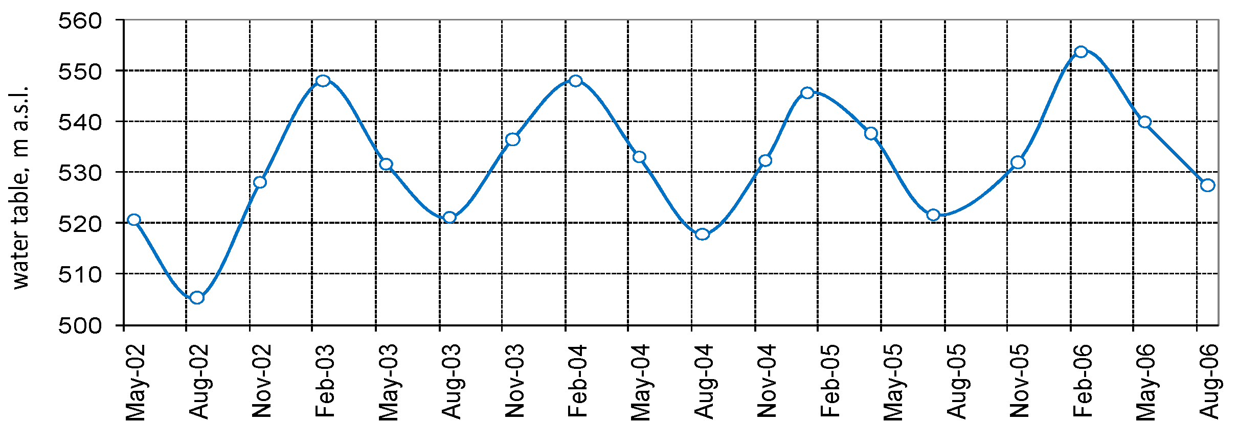
The water table of the saturated zone inside the karst area can be measured in several wells and piezometers located in the Piana del Dragone, which can be considered as the main recharge zone of the aquifer. Locally, the water level has a mean of 530 m a.s.l. (period from 2002–2006, Figure 4), and can be considered as the higher elevation of the basal water table in the Terminio massif; this level is 150 and 55 m higher than the Acquaro-Pelosi and Cassano springs, respectively. On the basis of the measured data (water level has been measured every three months), the water table level increases during the recharge phase (autumn and winter) and decreases in late spring/summer.
The Serino Spring Area
Between the villages of S. Lucia and S. Michele di Serino, many springs exist which rapidly increased the discharge of the Sabato River. After drainage works to tap these springs, only few resurgence phenomena can be observed along the river, which are negligible during the low flow season.
In the Urciuoli springs zone (approximately 330 m a.s.l.), there are three drainage tunnels (North, West and Main channels) that convey the water towards a storage tank. From this point, a gravity channel, followed by a system of pressured conduits, supply Naples urban area [25].
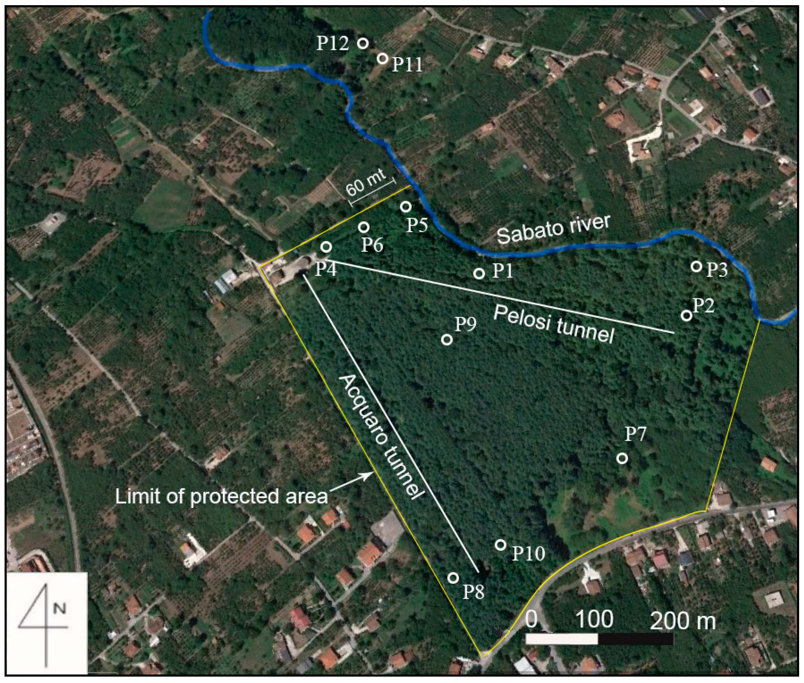
The Acquaro-Pelosi springs area is located 3 km uphill of Urciuoli springs (Figure 3 and Figure 5), in a flat area along the Sabato River (370–380 m a.s.l.). Uphill this area, the Sabato River is completely dry, and it is only after rainy days that the runoff can occur. Before the tapping, numerous spring outlets existed locally; the construction of tunnels in 1934 has tapped most of these springs, and only a few spring points discharge after wet periods.
The two tunnels are excavated into alluvial deposits, they are 400 m long, and 4 to 7 m deep. Water is drained through loopholes in the concrete structure of tunnels along their bases and sides. The tunnels convey water to a storage tank, then toward Urciuoli springs.
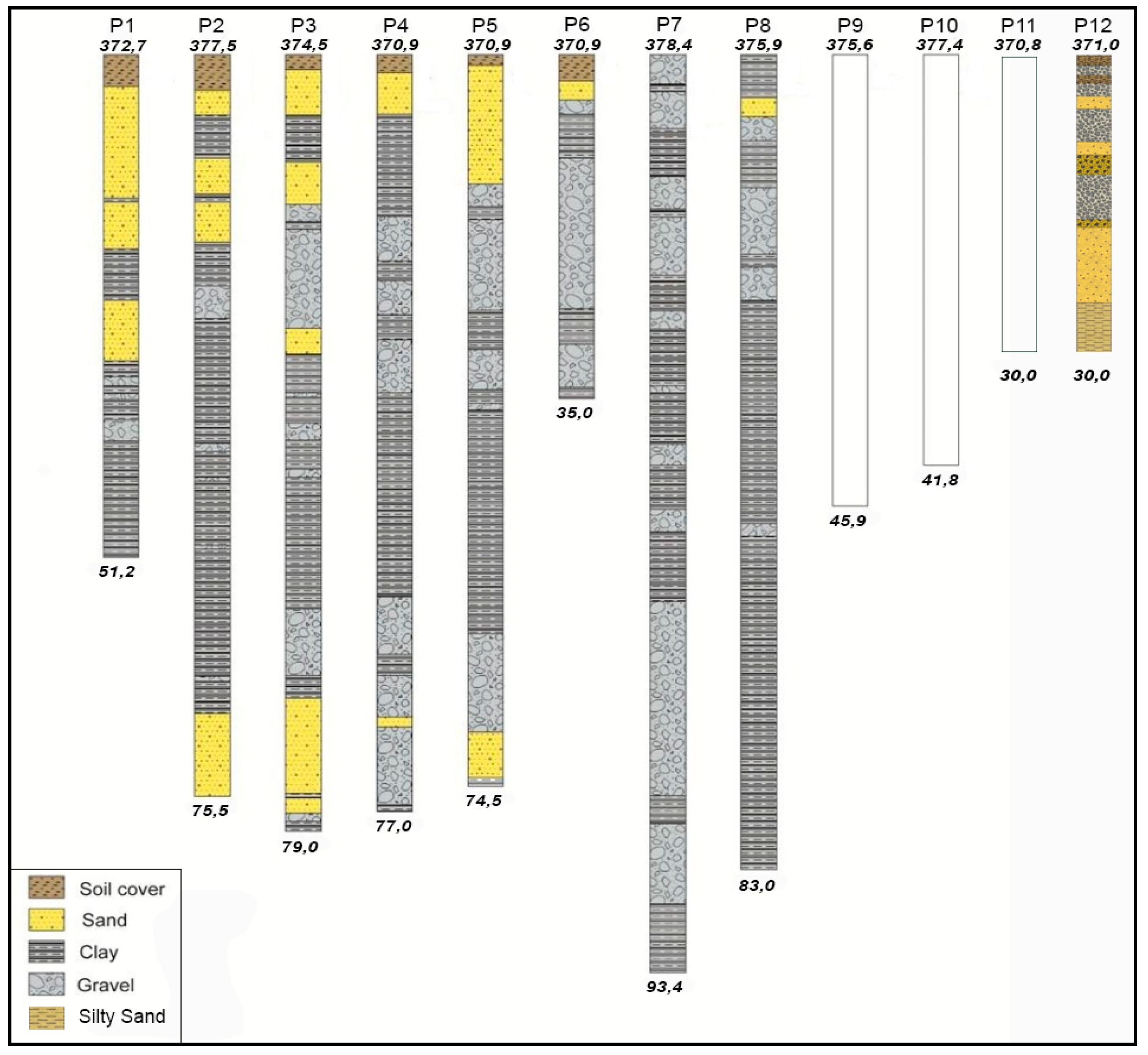
Ten wells are located inside the protected area, around the two drainage tunnels (Figure 5), and have depths between 30 m and 93 m. They cross the alluvial deposits constituted by sands, gravels and clays (Figure 6). Inside each well, a piezometer tube has been placed, which is slotted at the bottom part; this means that the water level measured into the piezometer has to be connected to the hydraulic head at the bottom part.
The entire water discharged by the Serino springs (mean of 2.25 m3/s) is linked to a deep karst substratum connected to a recharge area of the Terminio massif. In the Acquaro-Pelosi spring area, the karst substratum has not been reached by wells, and thus it lies below the deepest piezometer (>93.40 m).
Following the Geological map of Italy (ISPRA 2017), the karst substratum is believed to lie about 400 m deep in the Sabato Valley, but this depth is considered variable, reaching locally the minimum in correspondence to springs. In any case, all spring water comes from the upwelling flux inside the alluvial deposits of the Sabato plain, and these characteristics are further detailed.
4. Data Analysis
4.1. Hydrological Data and Correlations
Spring discharge measurements have been carried out by automatic hydrometers located along the hydraulic system of tapping. The discharge is directly measured at the end of the Pelosi and Acquaro drainage tunnels; the discharge of Urciuoli spring is indirectly obtained from the discharge measurements carried out downstream.
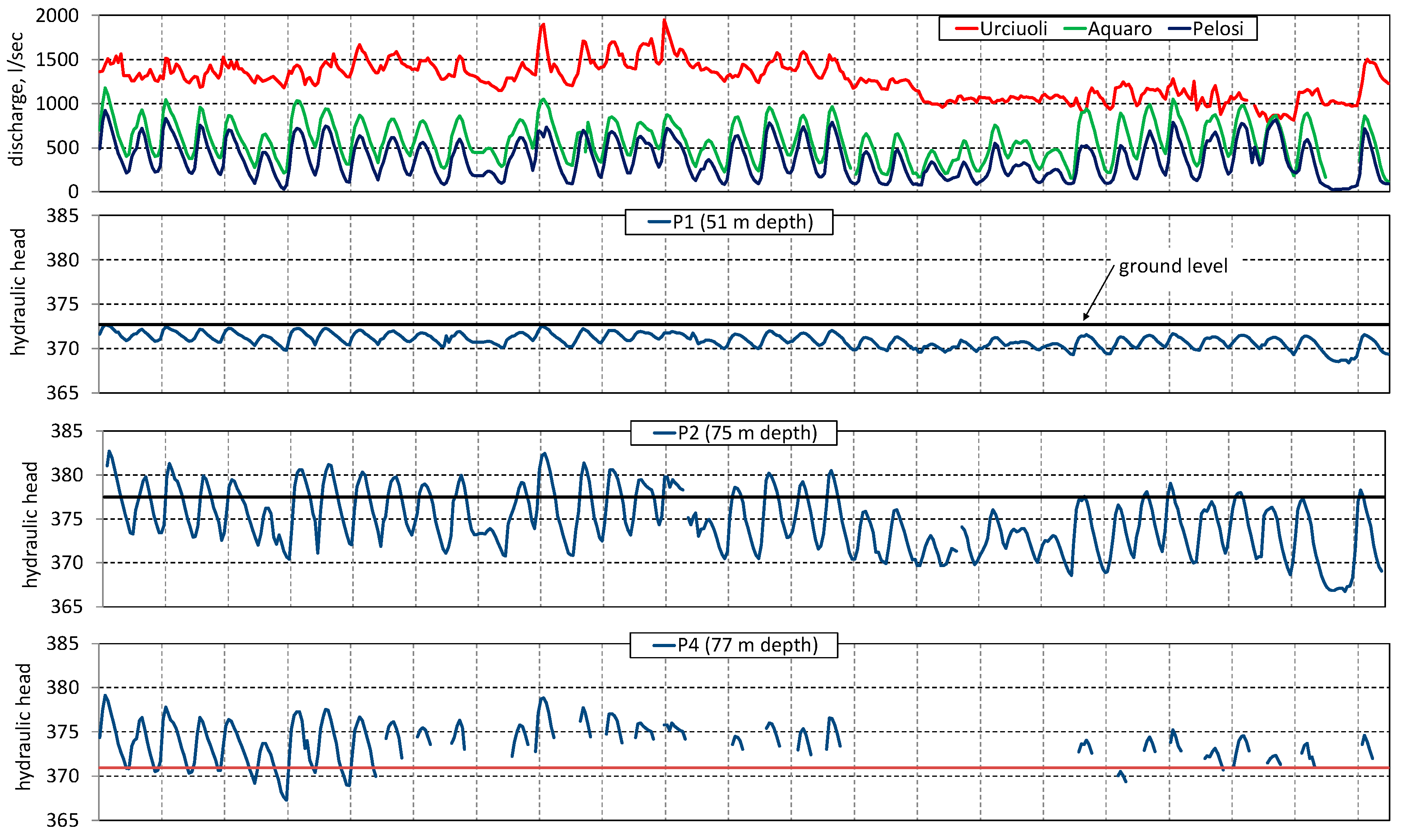
Figure 7 shows the hydrographs of the Pelosi, Acquaro and Urciuoli springs for the period 1963–2003; the minimum and maximum values occur in spring and autumn-winter seasons, respectively; during droughts, the spring hydrographs are characterized by a continuous decreasing trend for the entire hydrological year, as occurred in 2002 [28].
Fiorillo et al. [25] described the long time series of the Serino spring discharge and its relationship with climate (rainfall and temperature) variables. By cross-correlation analyses, they found strong dependence of spring discharge cumulative rainfall to be over 150 days, with time-lag of 2 months [25]. Besides, they focused on the minimum amount of rainfall needed to avoid a groundwater drought, thereafter, their statistical occurrence was estimated [25].
Piezometer level data considered in this study spanned the period of 1963–2003 as shown in Figure 7. For the piezometer P1, P2, P3, P7, P8, P9 and P10, data are almost continuous, whereas for piezometers P4, P5 and P6 data series present many discontinuities. In particular, these discontinuities occurred during low flow periods when these piezometers are used to tap the water conveyed to the storage tank.
Besides, the piezometric level can be artesian during the high flow period, as observed in piezometers P2, P3, P4, P5 and P7; these piezometers are also the deepest.
The P4 and P5 piezometers are also under artesian conditions also during low flow periods except for a few years of extreme drought (for example 2002). In the shallower piezometers P1, P9 and P10, the hydraulic head is always below the ground level.
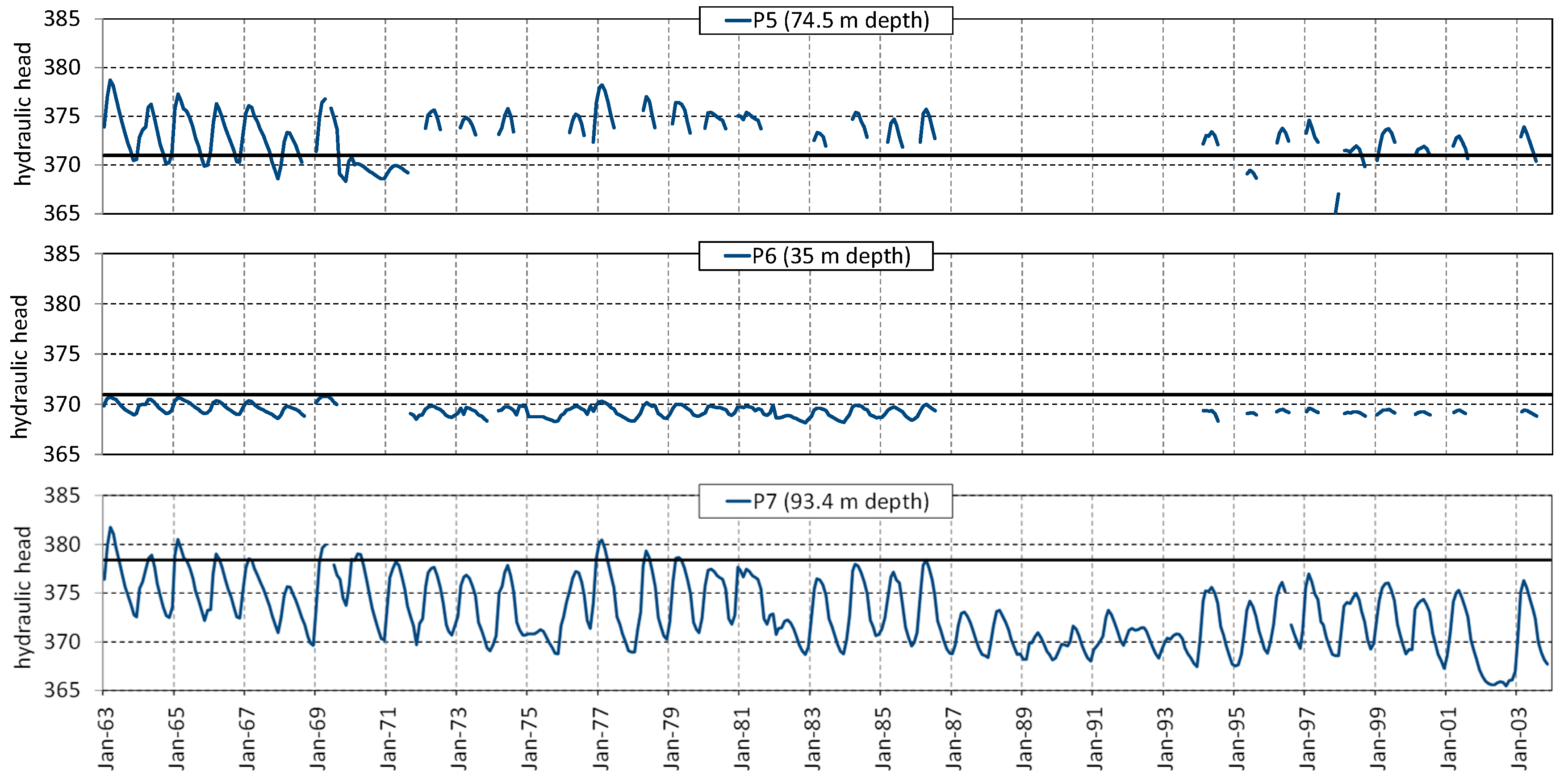
Figure 8 shows in detail the hydraulic head of piezometers during the period 1963–1969, during which records are available almost continuously. The deepest wells (P2, P3, P4, P5, P7) have a higher hydraulic head, especially during the high flow period of springs (March–July). During the low flow period of springs (September–November), these wells present a drop in the hydraulic head, which decreases below that of the shallowest wells (P1, P10).
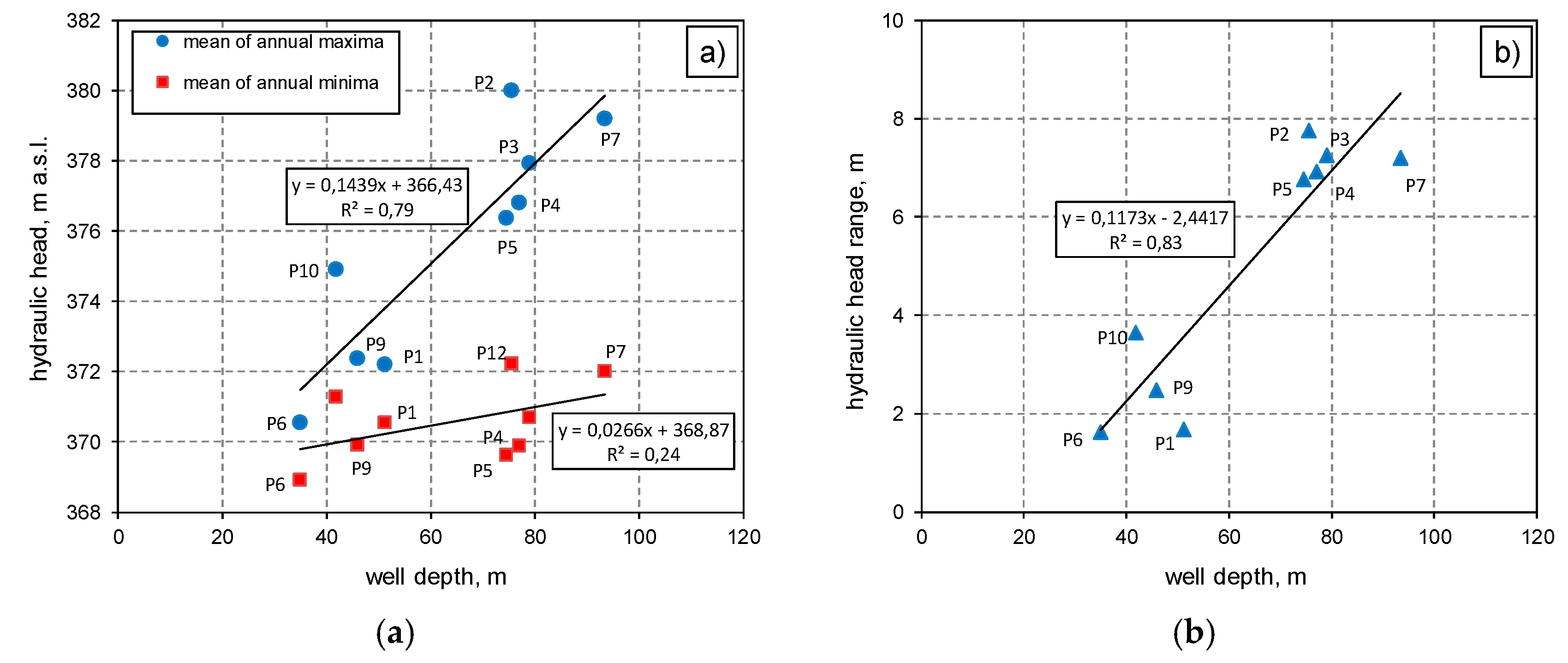
As can be deduced from Figure 8, the distribution of the hydraulic head into the alluvial deposits is not phreatic, as it generally increases in depth. In fact, the deepest piezometers show a higher hydraulic head than the shallower piezometers, especially during the April–June period. These characteristics are shown in Figure 9, with data plotted as mean values in the period 1963–1969, during which a continuous record occurred for all piezometers. The dependence of the hydraulic head on the piezometer depth is obvious (Figure 9a), as well as the hydraulic head range (Figure 9b). The piezometer P8, which is drilled mainly in the clayey deposits at the bottom part (Figure 6), is not shown in Figure 8 and Figure 9.
To assess the aquifer’s transmissivity, permeability and specific yield, a multi-purpose aquifer test was carried out on pumping well and monitored piezometer (P11 and P12, Figure 5).
The test was carried out at a constant pumping rate of 38.5 L/s, for a duration of 68 h; drawdown data were processed using the method of Neuman [29], enhanced by Tartakovsky and Neuman [30]. Results are shown in Table 1; the hydraulic conductivity, K = 3 × 10⁻³ m/s and the effective porosity, neff = 0.1, are in line with lithostratigraphic and granulometric features.
4.2. Physical and Chemical Characteristics
The total dissolved solids values are 221 mg/Kg and 201 mg/Kg for Acquaro-Pelosi and Urciuoli respectively and it results in the poor mineralization of water. The main ions are the calcium (++Ca, 65 mg/L) and the hydrogen carbonate (−HCO3, 240 mg/L) according to origin of water for karst aquifer.
A set of monthly temperature and electrical conductivity measurements have been carried out within the period of March 2015–July 2016, for Acquaro, Pelosi and Urciuoli springs (Figure 10a).
The electrical conductivity appears almost constant for the Pelosi spring, where a value of 350 μS/cm is observed for the entire period. In the Acquaro and Urciuoli springs a range between 450 and 350 μS/cm is recorded in the same period. The temperature shows constant values around 10.5 °C (Acquaro and Pelosi) and 11 °C (Urciuoli); while during the recession period (August–November) an increase of 1–2 degrees is observed.
In the same period (February 2015–July 2016) a monthly 222Radon concentration measurements were carried out for the Acquaro, Pelosi and Urciuoli springs. Figure 10b shows the results obtained from 222Rn activity together with the discharge values, where a clear and similar trend can be observed. A significantly positive linear relationship results from a comparison between spring discharge and 222Rn activity, indicating the strong control of the hydrological cycle on the radon concentration.
5. Results
The correlations of Figure 9 indicate that the hydraulic behavior of the alluvial aquifer is characterized by an upwelling flux during the high flow period, where the slope of the interpolation line (equation y = 0.1439x + 366.43, Figure 9a) can be assumed as a first coarse estimation of the hydraulic gradient, ia. Due to the non-isotropic behavior of the alluvial deposits, this hydraulic gradient has to be assumed as the mean value of the ascendant flow into alluvial deposits during the high flow period.
During the low flow period, the behavior appears more complicated. Considering the mean of annual minima (Figure 9a), an ascendant hydraulic gradient can be roughly estimated by the slope of the interpolation line (equation y = 0.0266x + 368.43; Figure 9a), but the correlation is weaker. In fact, during the recession period, the hydraulic head of some deep piezometers decreases up to values lower than shallower piezometers (Figure 8). Thus, during the low flow period, the flux could have a descendant component into some portions of the alluvial deposits; under such conditions, the alluvial aquifer can feed the springs (drainage tunnels).
Another main consideration can be done as shown Figure 9b: the hydraulic head range appears to be clearly dependent on the depth of the well, indicating a wider oscillation of the hydraulic head into deepest deposits.
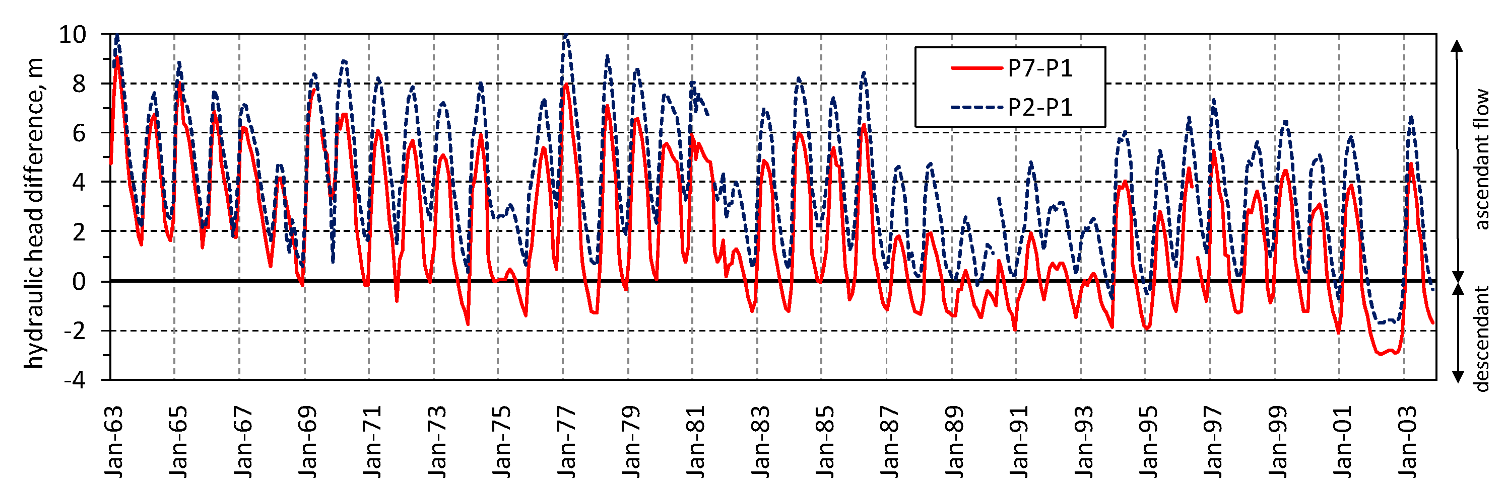
To investigate the aquifer behavior and its possible “reverse” behavior (descendant flux), the difference in hydraulic head between P7 and P1 (P7−P1), and between P2 and P1 (P2−P1) have been plotted as shown in Figure 11; these piezometers have almost complete records in the period between 1963–2003, and allow for comparison a deep (P7 and P2) and shallow (P1) piezometer. Observing the difference between P7 and P1 (P7−P1), it seems that the “reverse” period occurs every year since 1987; whereas, observing the difference between P2 and P1 (P2−P1), the “reverse” period would be limited to the drought of 2002 and to other few and short periods. Figure 11 indicates that the “reverse” condition would be very limited in time and space, and that probably it is only a misleading result due to a comparison of the hydraulic head measured into two distinct piezometers, and not along the same vertical. Observing Figure 10a, the slight temperature increase between August and November could indicate the possible mixing between deep (ascendant flow) and shallow water of alluvial aquifer, but the electrical conductivity does not change.
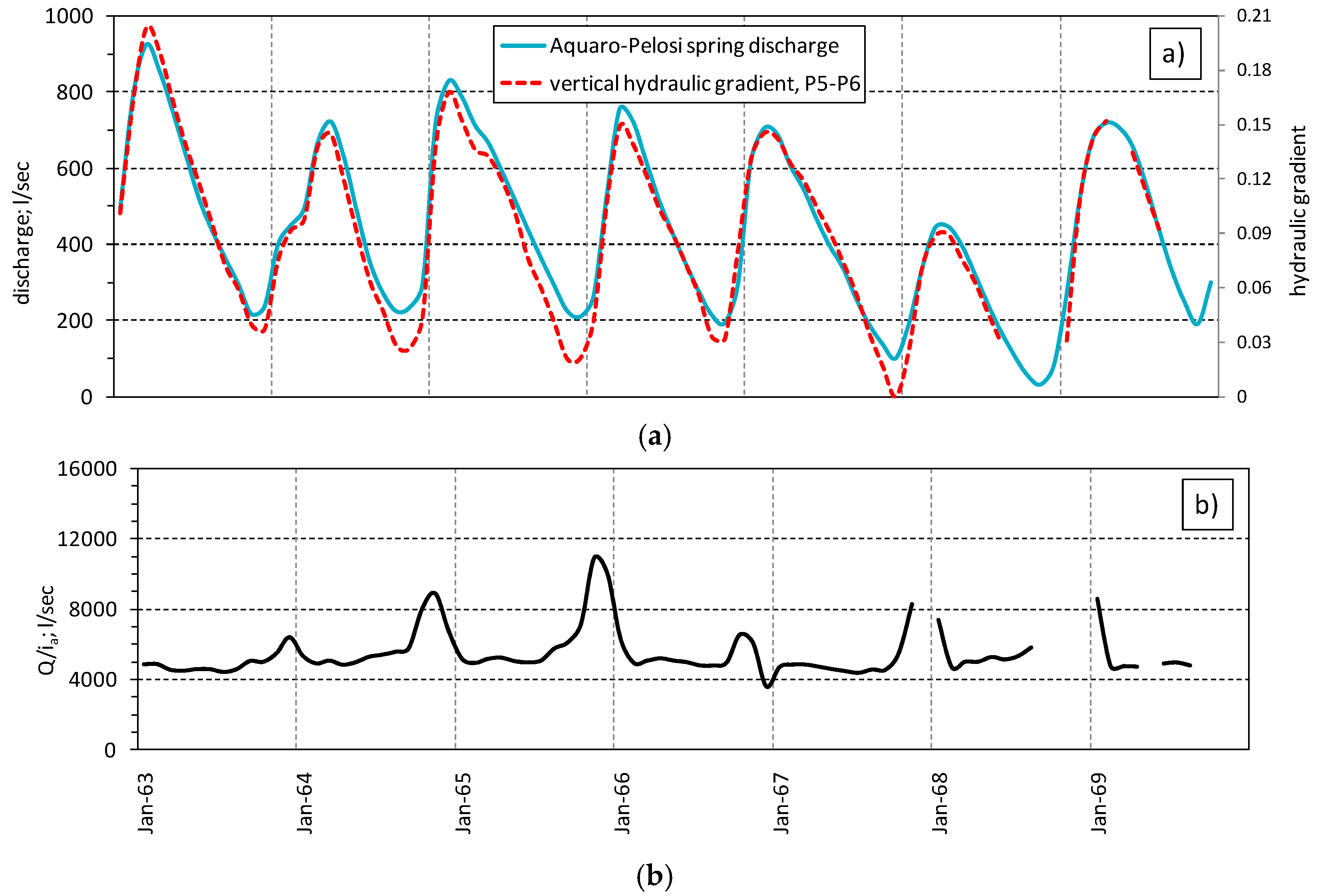
To reduce the ambiguity observed in Figure 11, the ascendant hydraulic gradient has been estimated by considering two close piezometers, characterized by different depths. For this reason, the analysis is restricted to piezometer P5 and P6; P4 could replace P5 (it is far from P6 as P5, and has a depth comparable with P5) providing similar results. The estimated ascendant hydraulic gradient into alluvial deposits is shown in Figure 12, where it is well-correlated with the discharge. In this case, the hydraulic gradient is always positive (ascendant flow), and it increases or decreases during the high flow and low flow periods, respectively. It has to be specified that the actual hydraulic gradient could be up higher with respect to that computed because of the uncertainty in the hydraulic isolation of the piezometric tube.
Plotting the ratio between the spring discharge and hydraulic gradient, Q/ia (Figure 12b), a constant path can be observed, which is interrupted by a peak during low flow periods. Following the Darcy law:
with K being the hydraulic conductivity, and A the area, the plot of Figure 12b means that during low flow periods, the area, A, has to increase proportionally to ratio Q/ia, as the hydraulic conductivity, K, can be considered constant. It has to be specified that the area, A, lies on the horizontal plane in this case, as the flow lines are vertical under the ascendant hydraulic flow into the aquifer. The area, A, increases or decreases under low and high ascendant hydraulic gradients, respectively; and to investigate this behavior, Figure 1b shows the effect of the drainage tunnel on the water table. The natural ascendant hydraulic flow causes the start-up of springs on the ground level; the drainage tunnel excavation induces a water table drop; the distance R defines the wideness of the influenced zone of the aquifer. To estimate the R-value under an ascendant hydraulic gradient condition, Equations (1) and (2) have been used.
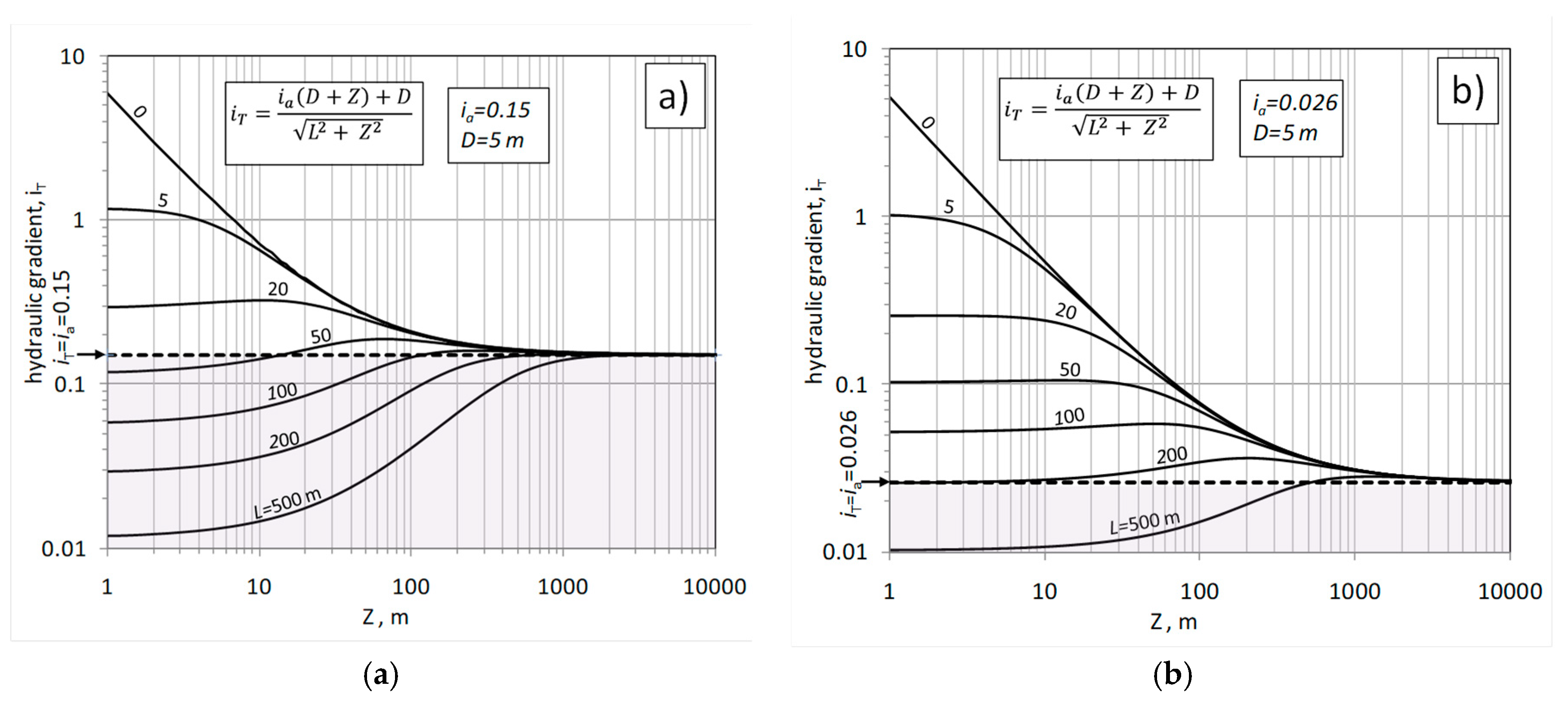
Figure 13 shows the plot of Equation (2), where the potential hydraulic gradient, iT, depends on the depth, Z, and distance, L, from the drainage/spring, distinguishing the condition under high (Figure 13a) and low (Figure 13b) ascendant hydraulic gradient, respectively; the hydraulic gradient values, ia = 0.15 and ia = 0.026, are the mean of the annual highest and lowest values in the period 1963–1969 (Figure 12a), and are similar to the slope of the interpolation line of Figure 9a.
As shown in Figure 13, the potential hydraulic gradient, iT, tend to ia when Z increases. The drainage towards the tunnel/spring occurs for iT > ia; in this case the ascendant flow converges to the tunnel/spring. In the field iT < ia, the ascendant flow continues its vertical path. The horizontal line iT = ia is a boundary limit, splitting the zones descripted above; along this line does the condition L ≡ R occur. In Figure 13a, for Z = 100 m the condition ia = iT occurs when L ≈ 100 m; in Figure 13b, for Z = 100 m, the same condition occurs when 200 < L < 500 m; these theoretical results are in accordance with the actual results of Q/i ratio (Figure 12b), where the area, A, has to increase under a low hydraulic gradient.
Equalizing Equations (1) and (2) by fixing ia = iT, the distance LP will coincide with R, and thus:
Figure 14 shows the dependence of the zone influenced by the drainage system (R-value) in the function of Z, for a different ascendant hydraulic gradient, ia, including the maximum and minimum observed (0.15 and 0.026). This relationship highlights how the depth, Z, of the ascendant flow lines control the R-value. As the depth of the karst substratum can be used as the maximum Z value, it can be estimated by comparing two different scenarios in Equation (4). In particular, as shown in Figure 12b, the area, A, increases n times from high flow to low flow condition, by the following:
and from Equation (4):
the value ZP deducted provides the depth of the karst substratum, ZK ≡ ZP. For n = 2.5, ZK = 353 m. This value of ZK is compatible with the geological and hydrogeological features of the study area; the correspondent values of R, are 169 and 422 m in conditions of high flow (ia = 0.15) and low flow (ia = 0.026) as shown in Figure 14.
6. Discussion
The relationship between groundwater and surface water has been discussed by Sophocleous [31], and by Barthel and Banzhaf [32] at a regional scale. In general, the presence of an ascendant flux could be very difficult to detect in many hydrogeological contexts. For example, in an alluvial plain characterized by sand deposits and ascendant water flux with vertical hydraulic gradient ia = 0.01, two distinct piezometers, close together, but having 10 m depth difference, would measure a hydraulic head difference of 0.1 m. This hydraulic head difference could be misleading of a prevalently horizontal flow, and similar considerations can also be provided for other aquifer types, karst included. The possibility of measuring and quantifying the ascendant hydraulic gradient depends on its magnitude and on the depth of the piezometers.
In some areas the ascendant flux has been detected due to a deep geological survey. For example, in the Crni Timok valley, Serbia, geophysical surveys by the spontaneous potential method (SP) has allowed for the identification of the zone characterized by an ascendant flux in the karstified limestone buried under alluvial deposits [33]. Besides, in the Duna-Tisza interfluves, Hungary, Szőnyi and Tóth [34] reconstructed the ascendant flux from deep water and hydrocarbon wells, which is responsible for severe problems of soil and wetland salinization.
In many karst aquifers of Southern Apennines the water table of the saturated zone is flat, and it is generally characterized by hydraulic gradient lower than 1% [35]; these conditions favor a deep water circulation, with flow lines converging to a spring outlet and characterized by vertical path (Figure 15a). The development of a conduit net into a karst aquifer leads to a hierarchical flow [36], which controls the water path; the ascendant flux can lead to the formation of subvertical conduits, and many karst springs are fed by a typical subvertical conduit, as the Vauclusian types. In these cases, tectonic shifts between karst terrains and aquiclude favor the formation of the subvertical conduit [37]. Many karst springs of Southern Italy can be associated with the scheme of Figure 15a, as Caposele spring of Picentini mountains or Boiano springs of Matese massif, where the conduit net (not drawn) leads the flow lines.
Many other karst springs emerge from carbonate rock block tectonically joined to a wider karst area (Figure 15b). The presence of no-karst terrains, which act as aquiclude or aquitard between the main aquifer and the rock block, favors the development of a deep groundwater flow, converging toward the rock block, which is interested in ascendant groundwater flux. In Southern Italy, Capovolturno spring of Meta mountains or Grassano spring of Matese massif is associated with the scheme of Figure 15b.
In many other cases, the carbonate rock-block is missing in outcropping and lies below the no-karst terrains (Figure 15c); springs can originate through ascendant fluxes into porous deposits, and faults allow for crossing the aquiclude/aquitard above the karst aquifer. Serino springs can be associated with the scheme of Figure 15c, which is common also to other karst springs of Southern Italy as Cassano springs along the eastern side of Terminio massif (Figure 3).
The hydrogeological cross-section of Figure 16 shows how the flux from the recharge area is forced under the aquiclude of flysch sequences; in the Sabato plain, the presence of springs has been explained by a buried karst substratum, covered by thick alluvial deposits. In the alluvial deposits, the flux is widespread and circulates in a porous medium; most of the upwelling flux outcrops along the Sabato River, located on the shorter and vertical flow line of the upwelling flux, and thus, along the buried fault system.
Inside the karst substratum, the limit between karstified and unkarstified terrains is unknown; this limit has been marked by question marks, and it could be fixed at −130 m below sea level, which was the base level during the last glaciation. However, as karstification processes began during the continental exposition of carbonate reliefs, deeper karst levels are lowered by Pliocene and Quaternary faults.
In the Piana del Dragone, which is the main recharge area of the aquifer (Figure 3), the hydraulic head varies between 506 m a.s.l and 554 m a.s.l. in the period between 2003–2008 (Figure 4); the observed range, Δh1 = 48 m, has been indicated in Figure 16. The hydraulic head in this area controls the hydraulic head observed in the piezometers of the Serino plain, which have a range up to 8 m (Figure 9b).
Under drought conditions, a descendant hydraulic gradient could occur in alluvial deposits, which means (i) a poor hydraulic head into karst substratum connected to a poor recharge and (ii) a temporary reverse flow into alluvial deposits which recharges the karst aquifer below. However, the above drought conditions occur rarely, and ascendant hydraulic gradient occurs during the entire hydrological year and supports the fact that the spring never dries up (except Acquaro spring during in the year 2002). A minimum and maximum hydraulic gradient (0.026 and 0.15, respectively), as previously estimated, will now be considered.
Figure 17 shows the hydraulic gradient estimated in depth, extrapolating the hydraulic head measured in P5 and P6 wells (Figure 12a); the top of the karst substratum can be estimated by Equation (6), and thus the hydraulic head ranges into karst substratum would be Δh1 ≈ 40 m. This value is slightly lower than 48 m found in well S1 located in the recharge zone (Figure 3, Figure 4 and Figure 16), according to water path into karst aquifer, from the recharge zone to karst substratum below the alluvial deposits. However, as data sets cover different periods, a more specific link between water level recorded in the Piana del Dragone (2002–2006) and piezometers of Sabato valley (1963–1969) could not be allowed.
A relevant consequence of high values of the ascendant hydraulic flow is the spring water quality. As described, this water is cold (T = 11 °C) and it is poorly mineralized (E.C. = 370 μS/cm, 20 °C), but it comes from a deep aquifer, located at 353 m depth below the Sabato River. We expected that water coming from so deep an aquifer should be more mineralized, as found in other hydrogeological contexts [34,38,39]. A possible explanation can be found in the high velocity of the ascendant flow into alluvial deposits directly connected to the high hydraulic gradient.
Using the results of a pumping test carried out in the P11 and P12 wells (Figure 5), which provided a hydraulic conductivity, K = 3 × 10⁻³ m/sec, a velocity of v = 1.62 m/h (i = 0.150, high flow) and v = 0.28 m/h (i = 0.026, low flow) can be estimated. Considering an effective porosity of 0.1 of the alluvial deposits (sand and gravel), the actual velocity is veff ≈ 16.2 m/h (high flow) and veff ≈ 2.8 m/h (low flow). This means that, during the high flow and low flow, water would need ≈1 day or ≈5 days to reach the springs from the karst substratum, respectively, and within this short period there is a better understanding as to why the Serino spring water is poorly mineralized and cold.
The 222Rn activity for Acquaro and Pelosi springs clearly indicate a variation in the concentration in the monitored period (February 2015–July 2016); in particular, as shown in Figure 10, 222Rn activity clearly increases as spring discharge increases, and decreases as spring discharge decreases; maximum and minimum radon activities occur during the high and low flow conditions, respectively.
The high flow condition is sustained by high ascendant hydraulic gradient, under which higher water velocity and higher radon activity occur. Thus, the high velocity of the upwelling flow allows a more rapid ascendant water which favors a higher 222Rn activity. During low flow periods, when a lower ascendant flow occurs, the 222Rn activity decreases as consequence of the longer period it takes for water to reach the springs.
Moreover, the difference between the time needed to reach the spring from karst substratum during the high and low flow (≈4 days) coincides with the half-time of the 222Rn (3.8 days), and the radon activity measured during the high flow period almost double of that measured during the low flow period. These results suggest that radon activity of groundwater stored in the saturated zone of karst aquifer substratum can be considered almost constant during the year, as a consequence of the long-term equilibrium between its accumulation (from the decay of uranium and radio contained in the rocks) and its decay (with a half time of 3.8 days). In this case, the faster upwelling of spring water occurring during high flow periods favor higher radon activity, whereas, the slower upwelling of spring water occurring during low flow periods favor the radon decay and, thus, its reduced activity in the spring water.
7. Conclusions
The ascendant water flux which feeds the springs belong to a wide hydraulic phenomenon involving wide areas and deep portions of aquifers. It is always connected to specific hydrogeological conditions, coming from tectonic and geomorphologic evolution. In a karst environment, the ascendant flux can be particularly developed because of the carbonate dissolution along the shorter flow lines, characterized by the higher hydraulic gradient and forming karst conduits, as well as allowing the water flux to siphon under no-karst terrains. This phenomenon is still poorly quantified, as deep hydraulic measurements are generally missing.
The Serino spring area is a useful example of detecting and estimating the ascendant water flux, thanks to deep piezometers into alluvial deposits which cover a karst substratum and high values of the ascendant hydraulic gradient. The estimation of the ascendant hydraulic gradient during the high and low periods has provided an overall view of the phenomenon, allowing us to estimate the depth of the karst substratum in the Sabato plain and have a deeper knowledge of groundwater flow. During low flow conditions, a wider area appears to be influenced by the drainage systems with respect to high flow conditions. These specific characteristics have been quantified by analytical solutions to find the area being influenced by a drainage system under different geometrical and hydraulic features.
As a consequence of the ascendant flux, the Serino alluvial plain can be considered outside of the spring catchment, as it does not contribute in recharging the below karst aquifer. Besides, especially during the high flow period, the spring water could be exposed to contaminations by perched water in the alluvial plain, and ascendant flux appears to be a useful and natural condition for preserving deep groundwater. However, drought conditions reduce the power of the ascendant hydraulic gradient drastically, and spring discharge can decrease up to nil; thus, drought conditions could favor the deterioration of water quality.
The ascendant water flux allows deep groundwater to reach the surface and start up a spring, and thus it is a common condition for thermal springs and other mineralized waters. For the Serino springs, which are cold and very low mineralized water, it is assumed that the estimated ascendant velocity is high enough to avoid increases in temperature and mineralization. In particular, the time needed to reach the spring outlet has been estimated at one (high flow) or a few days (low flow) from the karst substratum, and this sheds light on the almost constant value of temperature and electrical conductivity. Under such hydraulic conditions, characterized by a general fast velocity of the groundwater, the 222Rn activity seems to be a useful indicator of groundwater dynamic; in detail, during high flow periods, the water is younger with respect to low flow periods, due to a higher ascendant flow velocity.
The recognized upwelling flux in the Serino plain could lead to a better understanding also of many karst springs of Apennine, when hydrogeological conditions can be schematized as shown in Figure 15. Under such hydrogeological conditions, the ascendant water flux has not been fully recognized. This could lead to a better vulnerability definition and, thus, a more efficient local planning in order to correctly manage and preserve the quantity and quality of groundwater resources.
Acknowledgments
Hydrological and chemical data have been provided by aqueduct companies of Naples (Acqua Bene Comune) and Avellino (Alto Calore Servizi). Thanks also to Domenico Cicchella, University of Sannio, for his support during the Radon activity measurements.
Author Contributions
Francesco Fiorillo has written the text and coordinated the research with Libera Esposito; Giovanni Testa has carried out is situ measurements and analyzed data series; Sabatino Ciarcia supported the geological aspects of the area; Mauro Pagnozzi developed some figures/maps and review some aspects of literature.
Conflicts of Interest
The authors declare no conflict of interest.
References
- Todd, D.K.; Mays, L.W. Groundwater Hydrology; Wiley: Chichester, UK, 2005; 636p. [Google Scholar]
- Stevanovic, Z.; Kresic, N. Groundwater Hydrology of Springs; Butterworth Heinemann-Elsevier: Oxford, UK, 2009; 592p. [Google Scholar]
- Hubbert, M.K. The theory of groundwater motion. J. Geol. 1940, 48, 785–944. [Google Scholar] [CrossRef]
- Toth, J. A theoretical analyses groundwater flow in small drainage basins. J. Geophys. Res. 1963, 68, 4795–4812. [Google Scholar] [CrossRef]
- Domenico, P.A.; Schwartz, F.W. Physical and Chemical Hydrogeology; John Wiley & Sons: Singapore, 1990; 824p. [Google Scholar]
- Martínez-Santos, P.; Díaz-Alcaide, S.; Castaño-Castaño, S.; Hernández-Espriú, A. Modelling discharge through artesian springs based on a high resolution piezometric network. Hydrol. Process. 2014, 28, 2251–2261. [Google Scholar] [CrossRef]
- Ford, D.; Williams, P. Karst Hydrogeology and Geomorphology; Wiley: Chichester, UK, 2007; 562p. [Google Scholar]
- Stevanovic, Z. Characterization of Karst Aquifer. In Karst Aquifers—Characterization and Engineering; Stevanovic, Z., Ed.; Springer: Berlin/Heidelberg, Germany, 2015; 692p. [Google Scholar]
- Blyth, F.G.H.; De Freitas, M.H. A Geology for Engineers, 7th ed.; Arnould Ed.: London, UK, 1984; 325p. [Google Scholar]
- Hooghoudt, S.B. Bijdragen tot de Kennis van eenige Natuurkundige Grootheden van de Grond; Verslagen van Landbouwkundige Onderzoekingen Algemeene Landsdrukkerij: The Hague, The Netherlands, 1940. [Google Scholar]
- Van Schilfgaarde, J. Design of tile drainage for falling water tables. J. Irrig. Drain. Div. 1963, 89, 1–12. [Google Scholar]
- Mishra, G.C.; Singh, V. A new drain spacing formula. Hydrol. Sci. J. Sci. Hydrol. 2007, 52, 338–351. [Google Scholar] [CrossRef]
- Lei, S. An analytical solution for steady flow into a tunnel. Ground Water 1999, 37, 23–26. [Google Scholar] [CrossRef]
- El Tani, M. Circular tunnel in a semi-infinite aquifer. Tunn. Undergr. Space Technol. 2003, 18, 49–55. [Google Scholar] [CrossRef]
- El Tani, M. Helmholtz evolution of a semi-infinite aquifer drained by a circular tunnel. Tunn. Undergr. Space Technol. 2010, 25, 54–62. [Google Scholar] [CrossRef]
- Park, K.H.; Owatsiriwong, A.; Lee, J.G. Analytical solution for steady-state groundwater inflow into a drained circular tunnel in a semi-infinite aquifer: A revisit. Tunn. Undergr. Space Technol. 2008, 23, 206–209. [Google Scholar] [CrossRef]
- Butscher, C. Steady-state groundwater inflow into a circular tunnel. Tunn. Undergr. Space Technol. 2012, 32, 158–167. [Google Scholar] [CrossRef]
- Vitale, S.; Ciarcia, S. Tectono-stratigraphic and kinematic evolution of the Southern Apennines/Calabria—Peloritani Terranesystem (Italy). Tectonophysics 2013, 583, 164–182. [Google Scholar] [CrossRef]
- Cinque, A.; Patacca, E.; Scandone, P.; Tozzi, M. Quaternary kinematic evolution of the Southern Apennines. Relationship between surface geological features and deep lithospheric structures. Ann. Geophys. 1993, 36, 249–260. [Google Scholar]
- Fiorillo, F.; Pagnozzi, M.; Ventafridda, G. A model to simulate recharge processes of karst massifs. Hydrol. Process. 2015, 29, 2301–2314. [Google Scholar] [CrossRef]
- Calcaterra, D.; Ducci, D.; Santo, A. Aspetti geo-meccanici ed idrogeologici nel settore sud-orientale del, M.te Terminio (Appennino Meridionale). Geol. Romana 1992, 30, 125–134. [Google Scholar]
- Celico, P. Schema Idrogeologico dell’Appennino Carbonatico Centro-Meridionale; Memorie e Note Istituto di Geologia Applicata: Napoli, Italy, 1978; Volume 14, pp. 1–43. [Google Scholar]
- Ciarcia, S.; Vitale, S. Sedimentology, stratigraphy and tectonics of evolving wedge-top depozone: Ariano Basin, southern Apennines, Italy. Sediment. Geol. 2013, 290, 27–46. [Google Scholar] [CrossRef]
- Civita, M. Idrogeologia del Massiccio del Terminio-Tuoro (Campania); Memorie e Note Istituto di Geologia Applicata: Napoli, Italy, 1969; Volume 11, pp. 5–102. [Google Scholar]
- Fiorillo, F.; Esposito, L.; Guadagno, F.M. Analyses and forecast of the water resource in an ultra-centenarian spring discharge series from Serino (Southern Italy). J. Hydrol. 2007, 36, 125–138. [Google Scholar] [CrossRef]
- Celico, P.; Magnano, F.; Monaco, L. Prove di Colorazione del Massiccio Carbonatico del Monte Terminio-Monte Tuoro; Notiziario Club Alpino Italiano: Napoli, Italy, 1982; Volume 46, pp. 73–79. [Google Scholar]
- Fiorillo, F.; Guadagno, F.M. Long karst spring discharge time series and droughts occurrence in Southern Italy. Environ. Earth Sci. 2012, 65, 2273–2283. [Google Scholar] [CrossRef]
- Fiorillo, F. Spring hydrographs as indicators of droughts in a karst environment. J. Hydrol. 2009, 373, 290–301. [Google Scholar] [CrossRef]
- Neuman, S.P. Effect of partial penetration on flow in unconfined aquifers considering delayed gravity response. Water Resour. Res. 1974, 10, 303–312. [Google Scholar] [CrossRef]
- Tartakovsky, G.D.; Neuman, S.P. Three-dimensional saturated-unsaturated flow with axial symmetry to a partially penetrating well in a compressible unconfined aquifer. Water Resour. Res. 2007, 43, W01410. [Google Scholar] [CrossRef]
- Sophocleous, M. Interactions between groundwater and surface water: The state of the science. Hydrogeol. J. 2002, 10, 52–67. [Google Scholar] [CrossRef]
- Barthel, R.; Banzhaf, S. Groundwater and surface water interaction at the regional-scale—A review with focus on regional integrated models. Water Resour. Manag. 2016, 30, 1–32. [Google Scholar] [CrossRef]
- Stevanovic, Z.; Dragisic, V. An example of identifying karst groundwater flow. Environ. Geol. 1997, 35, 241–244. [Google Scholar] [CrossRef]
- Szőnyi, J.M.; Tóth, J. A hydrogeological type section for the Duna-Tisza Interfluve. Hung. Hydrogeol. J. 2009, 17, 961–980. [Google Scholar] [CrossRef]
- Fiorillo, F.; Petitta, M.; Preziosi, E.; Rusi, S.; Esposito, L.; Tallini, M. Long-term trend and fluctuations of karst spring discharge in a Mediterranean area (central-southern Italy). Environ. Earth Sci. 2015, 74, 153–172. [Google Scholar] [CrossRef]
- Kiraly, L. Karstification and Groundwater Flow. In Evolution of Karst: From Prekarst to Cessation; Gabrovsek, F., Ed.; Zalozba ZRC: Ljubljana, Slovenia, 2002; pp. 155–190. [Google Scholar]
- Palmer, A.N.; Audra, P. Patterns of caves. In Encyclopedia of Cave and Karst Science; Gunn, J., Ed.; Fitzroy Dearborn: London, UK, 2004; pp. 573–574. [Google Scholar]
- Czauner, B.; Szőnyi, J.M.; Tóth, J.; Pogácsás, G. Hydraulic potential anomaly indicating thermal water reservoir and gas pool near Berekfürdõ, Trans-Tisza Region, Hungary. Cent. Eur. Geol. 2008, 51, 253–265. [Google Scholar] [CrossRef]
- Goldscheider, N.; Szőnyi, J.M.; Erőss, A.; Schill, E. Review: Thermal water resources in carbonate rock aquifers. Hydrogeol. J. 2010, 18, 1303–1318. [Google Scholar] [CrossRef]
Figure 1.
(a) Ascendant flux connected to artesian conditions of karst aquifer covered by alluvial deposits. Hydraulic head observed in close boreholes with different depths allow to estimate the ascendant hydraulic gradient, ia; (b) Sketch of estimation of the ascendant hydraulic gradient, ia, and of the potential hydraulic gradient, iT, in the point P; HP, excess of hydraulic head of the point P respect to undisturbed water table; D, elevation difference between undisturbed water table and drainage system; R, width of water table involved by drainage (influenced zone); LP, horizontal distance of P from drainage; ZP, depth of P from drainage; ZK, depth of the karst substratum.

Figure 2.
Geological sketch of Southern Appennines (from [23], modified).
Figure 2.
Geological sketch of Southern Appennines (from [23], modified).

Figure 3.
Terminio massif hydrogeological map (location in Figure 2): (1) cover deposits (Quaternary) with medium-high permeability (slope breccias and debris, pyroclastic, alluvial and lacustrine deposits); (2) no-karst terrains with low permeability (argillaceous complex and flysch sequences of Paleogene–Miocene); (3) karst terrains (calcareous-dolomite series of Jurassic–Miocene); (4) Towns; (5) main karst springs; (6) elevation points (m a.s.l.); (7) mountain peak; (8) AA’ section line; (9) S1 monitored well. Dashed rectangle area is detailed in Figure 5.

Figure 4.
Water table level measured every three months in well S1, located in the Piana del Dragone (Figure 3, well head 686 m a.s.l.).
Figure 4.
Water table level measured every three months in well S1, located in the Piana del Dragone (Figure 3, well head 686 m a.s.l.).

Figure 5.
Aerial view of discharge area of Acquaro-Pelosi springs (dashed rectangle area of Figure 3), currently tapped by the drainage tunnels, and piezometers location (P1–P12).
Figure 5.
Aerial view of discharge area of Acquaro-Pelosi springs (dashed rectangle area of Figure 3), currently tapped by the drainage tunnels, and piezometers location (P1–P12).

Figure 6.
Well logs located in Figure 5; the ground elevation (m a.s.l.) and the depth (m), are shown above and below the lithostratigraphic column, respectively.
Figure 6.
Well logs located in Figure 5; the ground elevation (m a.s.l.) and the depth (m), are shown above and below the lithostratigraphic column, respectively.

Figure 7.
Discharge of Urciuoli, Acquaro and Pelosi springs, and piezometric levels measured in P1, P2, P4, P5, P6 and P7, during the period 1963–2003; values above the thick horizontal line (ground level) highlights artesian conditions.
Figure 7.
Discharge of Urciuoli, Acquaro and Pelosi springs, and piezometric levels measured in P1, P2, P4, P5, P6 and P7, during the period 1963–2003; values above the thick horizontal line (ground level) highlights artesian conditions.


Figure 8.
Hydraulic head during the period of 1963–1969, characterized by almost continuous records.
Figure 8.
Hydraulic head during the period of 1963–1969, characterized by almost continuous records.

Figure 9.
(a) Correlation between well depth and hydraulic head during high (mean of annual maxima, period between 1963–1969) and low flow periods (mean of annual minima, period 1963–1969); (b) Correlation between well depth and hydraulic head range (mean values, period between 1963–1969).
Figure 9.
(a) Correlation between well depth and hydraulic head during high (mean of annual maxima, period between 1963–1969) and low flow periods (mean of annual minima, period 1963–1969); (b) Correlation between well depth and hydraulic head range (mean values, period between 1963–1969).

Figure 10.
(a) Temperature and electrical conductivity, period between March 2015–July 2016, for Acquaro, Pelosi and Urciuoli springs, period between February 2015–July 2016; (b) Radon (222Rn) activity and spring discharge, period between February 2015–July 2016.
Figure 10.
(a) Temperature and electrical conductivity, period between March 2015–July 2016, for Acquaro, Pelosi and Urciuoli springs, period between February 2015–July 2016; (b) Radon (222Rn) activity and spring discharge, period between February 2015–July 2016.

Figure 11.
Hydraulic head difference between piezometers P7 and P1 (P7−P1) and piezometers P2 and P1 (P2−P1); positive and negative value means ascendant and descendant flow, respectively.
Figure 11.
Hydraulic head difference between piezometers P7 and P1 (P7−P1) and piezometers P2 and P1 (P2−P1); positive and negative value means ascendant and descendant flow, respectively.

Figure 12.
(a) Acquaro-Pelosi spring discharge and vertical (ascendant) hydraulic gradient, computed between P5 and P6 (60 m distance from each other; Figure 5); (b) ratio between discharge and hydraulic gradient (Q/ia).
Figure 12.
(a) Acquaro-Pelosi spring discharge and vertical (ascendant) hydraulic gradient, computed between P5 and P6 (60 m distance from each other; Figure 5); (b) ratio between discharge and hydraulic gradient (Q/ia).

Figure 13.
Potential hydraulic gradient, iT, induced by drainage system at depth D, computed along the vertical, Z, with distance L from drainage (Figure 1b): (a) aquifer with natural ascendant hydraulic gradient, ia = 0.15; (b) aquifer with natural ascendant hydraulic gradient, ia = 0.026. The drainage toward the tunnel/spring occurs in the field iT > ia; for iT < ia the ascendant flux is not influenced by the drainage.

Figure 14.
Width of the influenced zone, R, induced by drainage system at depth D, in relation to depth, Z, and for a different ascendant hydraulic gradient, ia. ZK is the depth of karst substratum.
Figure 14.
Width of the influenced zone, R, induced by drainage system at depth D, in relation to depth, Z, and for a different ascendant hydraulic gradient, ia. ZK is the depth of karst substratum.

Figure 15.
Ascendant flux connected to different hydrogeological conditions of the discharge zone of karst aquifers. (a) flow lines tend to be vertical as consequences of deep groundwater flow and flat water table; (b) no karst-terrains between the recharge and discharge area favors groundwater syphoning; (c) the hydraulic head difference, h1, is needed to allow the rising of groundwater through the porous medium from buried karst substratum.

Figure 16.
Hydrogeological section crossing discharge and recharge area of the Acquaro and Pelosi springs (section trace in Figure 3). Δh1 is the variation in the water table level in the phreatic zone (well S1), which becomes artesian in the Sabato valley. The limit of the karstification/saturated zone is unknown. R is the width of the influenced zone during high flow period (R = 169 m; Figure 14).

Figure 17.
Hydraulic head measured into wells P5 and P6 during high and low flow periods; the extrapolation in depth allow to estimation of the hydraulic head range, Δh1, in the karst substratum.
Figure 17.
Hydraulic head measured into wells P5 and P6 during high and low flow periods; the extrapolation in depth allow to estimation of the hydraulic head range, Δh1, in the karst substratum.


Table 1.
Main granulometry characteristics of soils (Unified Soil Classification System—USCS) and some hydraulic parameters obtained by pumping test carried out in well P12. Diameter, φ of soil: gravel, φ > 2 mm; sand, 0.06 mm < φ < 2 mm; silty and clay, φ < 0.06 mm. T, transmissivity; K, hydraulic conductivity; neff, effective porosity.
| Strata | Soil Type USCS | Thick. m | Gravel % | Sand % | Silt & Clay % | T m2/s (2) | K m/s (2) | neff- (2) |
|---|---|---|---|---|---|---|---|---|
| 1 | OL | 1.0 | ||||||
| 2 | GW (1) | 3.1 | ||||||
| 3 | SP | 1.3 | 32 | 66 | 2 | |||
| 4 | GW (1) | 3.3 | ||||||
| 5 | GW | 3.3 | 53 | 43 | 4 | |||
| 6 | GW (1) | 4.5 | ||||||
| 7 | SW | 8.5 | 35 | 58 | 7 | |||
| 8 | SM | 5.0 | 10 | 78 | 12 | |||
| ≈5 × 10⁻² | ≈3 × 10⁻³ | ≈0.1 |
Note: (1) Laboratory test missing, classification deducted from analogy with stratum n.5; (2) Results from pumping test in the well P12 (30 m depth)
© 2018 by the authors. Licensee MDPI, Basel, Switzerland. This article is an open access article distributed under the terms and conditions of the Creative Commons Attribution (CC BY) license (http://creativecommons.org/licenses/by/4.0/).
Share and Cite
MDPI and ACS Style
Fiorillo, F.; Esposito, L.; Testa, G.; Ciarcia, S.; Pagnozzi, M. The Upwelling Water Flux Feeding Springs: Hydrogeological and Hydraulic Features. Water 2018, 10, 501. https://doi.org/10.3390/w10040501
AMA Style
Fiorillo F, Esposito L, Testa G, Ciarcia S, Pagnozzi M. The Upwelling Water Flux Feeding Springs: Hydrogeological and Hydraulic Features. Water. 2018; 10(4):501. https://doi.org/10.3390/w10040501
Chicago/Turabian StyleFiorillo, Francesco, Libera Esposito, Giovanni Testa, Sabatino Ciarcia, and Mauro Pagnozzi. 2018. "The Upwelling Water Flux Feeding Springs: Hydrogeological and Hydraulic Features" Water 10, no. 4: 501. https://doi.org/10.3390/w10040501
Note that from the first issue of 2016, this journal uses article numbers instead of page numbers. See further details here.