Uncertainty of Rainfall Products: Impact on Modelling Household Nutrition from Rain-Fed Agriculture in Southern Africa
by
 , , and
Robert Luetkemeier
1,2,3,* ,
,
Lina Stein
4,
Lukas Drees
1,3,
Hannes Müller
5 and
Stefan Liehr
1,2,3 1
Institute for Social-Ecological Research (ISOE), Hamburger Allee 45, 60598 Frankfurt/Main, Germany
2
Southern African Science Service Centre for Climate Change and Adaptive Land Management (SASSCAL), 28 Robert Mugabe Avenue, 9000 Windhoek, Namibia
3
Senckenberg Biodiversity and Climate Research Centre (SBiK-F), Senckenberganlage 25, 60325 Frankfurt/Main, Germany
4
Faculty of Engineering, Senate House, University of Bristol, Tyndall Avenue, Bristol BS8 1TH, UK
5
Institute of Hydrology and Water Resources Management (IWW), Leibniz Universität Hannover, Appelstraße 9a, 30167 Hannover, Germany
*
Author to whom correspondence should be addressed.
Water 2018, 10(4), 499; https://doi.org/10.3390/w10040499
Submission received: 19 February 2018
/
Revised: 9 April 2018
/
Accepted: 9 April 2018
/
Published: 18 April 2018
Abstract
:Good quality data on precipitation are a prerequisite for applications like short-term weather forecasts, medium-term humanitarian assistance, and long-term climate modelling. In Sub-Saharan Africa, however, the meteorological station networks are frequently insufficient, as in the Cuvelai-Basin in Namibia and Angola. This paper analyses six rainfall products (ARC2.0, CHIRPS2.0, CRU-TS3.23, GPCCv7, PERSIANN-CDR, and TAMSAT) with respect to their performance in a crop model (APSIM) to obtain nutritional scores of a household’s requirements for dietary energy and further macronutrients. All products were calibrated to an observed time series using Quantile Mapping. The crop model output was compared against official yield data. The results show that the products (i) reproduce well the Basin’s spatial patterns, and (ii) temporally agree to station records (r = 0.84). However, differences exist in absolute annual rainfall (range: 154 mm), rainfall intensities, dry spell duration, rainy day counts, and the rainy season onset. Though calibration aligns key characteristics, the remaining differences lead to varying crop model results. While the model well reproduces official yield data using the observed rainfall time series (r = 0.52), the products’ results are heterogeneous (e.g., CHIRPS: r = 0.18). Overall, 97% of a household’s dietary energy demand is met. The study emphasizes the importance of considering the differences among multiple rainfall products when ground measurements are scarce.
1. Introduction
Precipitation, as the immediate source of water, is the most critical input variable of the water balance. For that reason, it is used in a wide array of models estimating hydrological variables, ranging from runoff and discharge, through drought intensity, down to impacts of climate change. An especially sensitive area of modelling is the estimation of agricultural yields and associated nutritional conditions, as decisions relating to food aid depend on these [1]. Due to the importance of precipitation in modelling, any inaccuracies in the input data will have a strong impact on estimated results and, thus, can directly compromise management decisions [2]. Errors in the spatial extrapolation of rainfall are often introduced because long-term time series from rain gauge stations, especially in poorly-equipped regions such as Sub-Saharan Africa (SSA), are rarely available [3]. Rainfall estimates derived from satellite-borne sensors or radar stations, therefore, provide a promising alternative in supplying near real-time precipitation data for large areas and long time series at fine spatial and temporal resolutions [4,5]. Nevertheless, the rainfall products (RPs) available are constructed with different sensor types and processing algorithms, resulting in uncertainties that have to be accounted for, since they impact on subsequent application stages [6]. In recent years, a number of studies have evaluated a range of rainfall products, in particular their application in hydrological [7,8,9,10] and agricultural models [11,12,13,14]. The studies confirm significant discrepancies in model output if uncalibrated rainfall products are used [12].
This becomes particularly relevant, if the yield estimations of agricultural models are used to support decision-making in critical tasks, such as emergency responses to humanitarian crises. Agricultural models can be used to estimate and monitor the nutritional situation and food security conditions in a certain area as partly build upon by the Famine Early Warning System Network (FEWS NET) [1]. Information on local food security conditions and the populations’ ability to meet their nutritional demand is particularly vital for aid organizations, governments and local agencies to identify people in need and act effectively, both in short-term emergency situations and in the context of long-term adaptation strategies.
The conditions in subsistence food systems can be described well via a range of nutritional status indicators [15] due to the direct link between agricultural yields and household nutrition. In Sub-Saharan Africa, rain-fed grain farming and livestock herding, known as mixed crop-livestock systems, remain the dominant livelihood strategy [16,17,18,19]. This is true for the majority of the population that still lives in rural settings [20]. Though urbanization processes and changing lifestyles are apparent, they largely depend on local hydro-climatic conditions to sustain their livelihood [21]. Despite evidence of progress towards the achievement of the Millennium Development Goals [22], the population is still challenged by high levels of poverty, non-inclusive economic growth, and low access to drinking water and sanitation infrastructures [23]. Recurring threats, such as droughts and famines, impact on the vulnerable population and result in a precarious situation of poverty persistence, civil conflicts, and food and water insecurity [18,24,25].
This paper analyses six commonly-used RPs with special emphasis on their spatial and temporal quality in comparison with sparsely available meteorological station records. As the exemplary study area, the semi-arid Cuvelai-Basin in Northern Namibia and Southern Angola is chosen, (i) as the RPs performances were not yet evaluated for this region, and (ii) it can be regarded as representative for many regions in SSA. For the purpose of estimating the degree of uncertainty that propagates through a modelling stage, the six daily RPs (CRU and GPCC were disaggregated from the monthly to the daily scale) are calibrated to observed rainfall data and subsequently used as input data for an exemplary crop growth model, the Agricultural Production Systems Simulator (APSIM) [26]. The model output of millet yield was transformed into nutritional scores of an average household’s requirements for dietary energy, proteins, lipids and carbohydrates. Official millet yield data from Central-Northern Namibia was used to validate the model results.
2. Materials and Methods
This study builds upon multiple public datasets and a range of processing methods that are presented in the following sub-sections. First, the Cuvelai-Basin as the exemplary study area is introduced. Second, the processing of the RPs is outlined against the backdrop of insufficient local rainfall station data. This is accompanied by a description of the calibration and disaggregation procedure used to adjust the products’ estimates. Third, the APSIM crop model is presented that facilitates the exemplary estimation of local staple food production. Finally, nutritional scores are introduced to characterize the nutritional situation of the local population.
2.1. Study Area
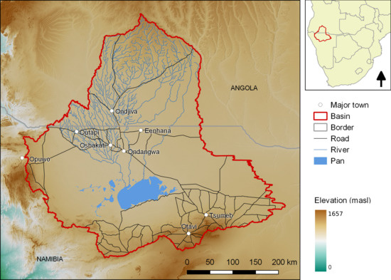
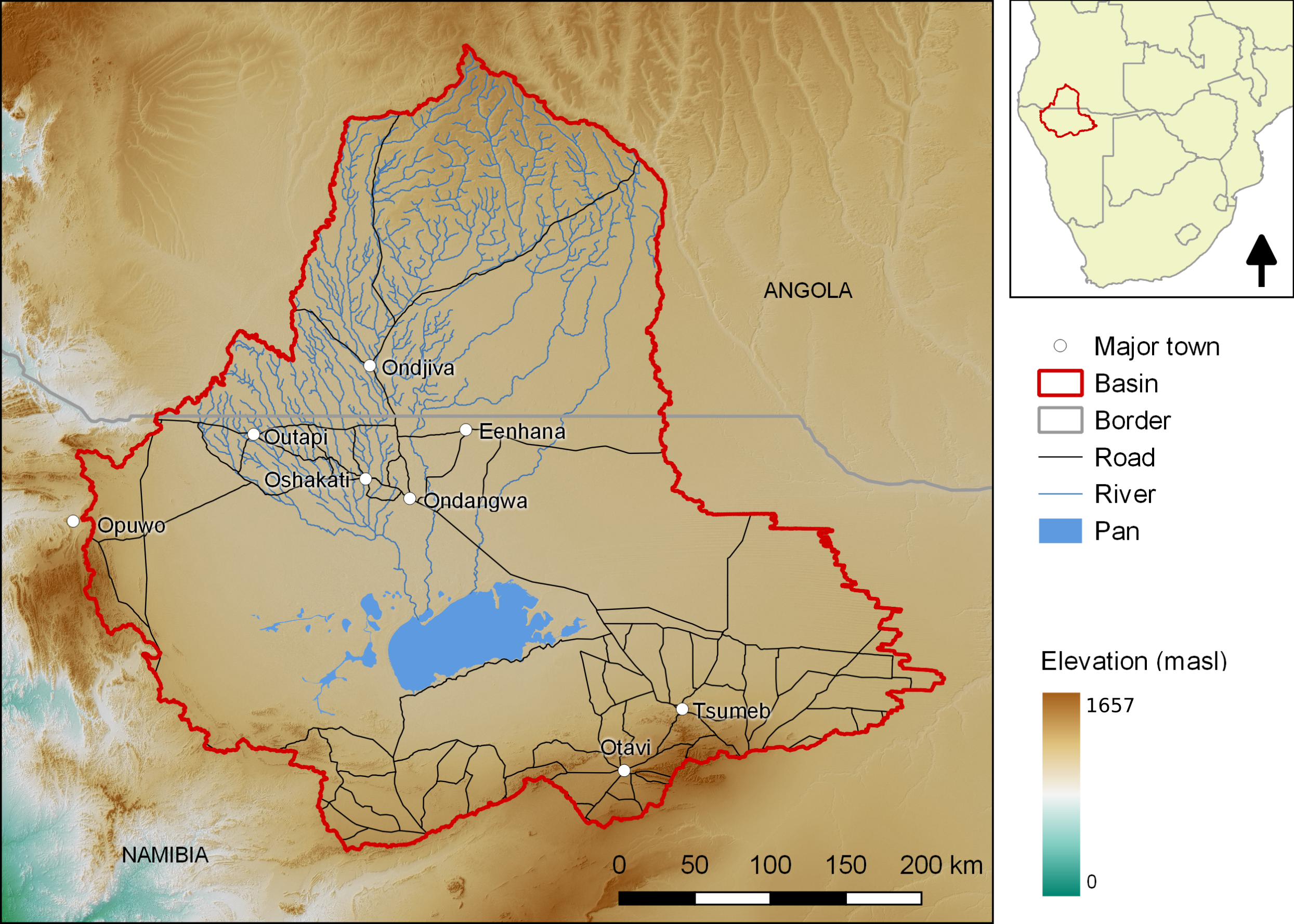
The Cuvelai-Basin is a transboundary, endorheic watershed that drains the Southern Angolan highlands into Central-Northern Namibia. It covers an area of approximately 172,000 km2, 31% of which belong to Angola and 69% to Namibia (Figure 1).
Most of the rivers are seasonal, especially between the towns of Ondjiva and Oshakati, where most of the population is located. Mean annual rainfall varies strongly across the basin with an increasing gradient from the southwest to the northeast. The central area has a mean annual rainfall depth of about 495 mm at the Okatana station, located in Central-Northern Namibia [31]. Seasonal variations in rainfall are typical, with a pronounced rainy season from October to April and a dry season in the southern hemispherical winter months. Inter-annual rainfall variability is high: numerous drought events were recorded in the late 1980s and mid-1990s, and also more recently between 2012 and 2015 [32], while ongoing drought conditions prevail due to the effects of El Niño. The total population of the basin on either side of the border is approximately 1.8 million [33,34] that mainly lives in rural areas with a high level of subsistence agriculture. Rain-fed farming of local varieties of pearl millet, inter-cropped with sorghum, maize, and a range of vegetables is the main agricultural activity. Taking rainfall onset variability into account, farmers use multiple planting dates from November/December through to January in order to minimize the risk of crop failure. Nevertheless, average yield is low with values between 100 and 400 kg/ha [35,36] which often only meets the domestic food demand on the household level. Livestock herding constitutes the second important pillar of livelihood activities and plays an important role in the socio-economic and cultural settings [27]. Local hydro-climatic conditions in this semi-arid environment are, thus, key to sustaining water and food security among a large section of the population [37].
2.2. Local Rainfall Observations
Good quality data on precipitation in terms of spatial and temporal coverage is a prerequisite for a range of applications, in particular hydrological and agricultural modelling [8,38,39]. Rain gauges are the primary and most reliable source of information on precipitation at a certain location, often measured via tipping-bucket techniques as one element of multi-purpose meteorological stations.
Meteorological station networks in Europe, North America, South Asia, and Australia provide particularly good spatial coverages and long time series spanning more than one hundred years [3]. Sub-Saharan Africa, however, does not have an extensive meteorological station network, and some regions have no station at all. However, this problem is not necessarily caused by a lack of infrastructural development. The Angolan civil war from 1975 to 2002 [40], for instance, coincides temporally with a massive drop in the availability of meteorological station records compared to the late 1960s when the country already enjoyed good station coverage [41]. The current distribution of meteorological stations within the Cuvelai-Basin is heterogeneous. Rainfall data from gauge measurements provided by the Namibian Meteorological Service [31] are available for the Namibian part of the Cuvelai. These time series have data gaps, but the information from a few stations near major settlements and the Etosha National Park in the central-north extends back to 1901. The Angolan part did not have any official stations, which is why the SASSCAL WeatherNet initiative (Southern African Science Service Centre for Climate Change and Adaptive Land Management) recently set up a number of meteorological stations in order to improve the monitoring infrastructure [41].
Since rain gauges provide point information, they only give a good indication of rainfall at a specific location. Reliable estimates for spatial rainfall patterns, however, require the interpolation of point information. Interpolation of rainfall is commonly performed using different methods, depending on the availability of station data, type of input, and auxiliary information. On the one hand, univariate methods, such as inverse distance weighting (IDW), Thiessen polygons, or Ordinary Kriging, are simple to apply and only require precipitation as an input variable. On the other hand, multivariate models, such as geographically-weighted regression or artificial neural networks, are more complex and require additional information, since they incorporate further explanatory variables, such as elevation [39]. While the more complex, multivariate interpolation schemes have been found to provide good results, IDW is a common interpolation method for monthly and annual precipitation data [39,42] and provides sufficient results for the purpose of this study. The IDW technique builds upon the spatial correlation of rainfall occurrence, meaning that the validity of point data is reduced with increasing distance from its source location. The measured rainfall depth at location is, thus, weighted () with the distance between the station’s location and the ungauged point of interest [39]. The interpolated rainfall for a specific location in between stations can thus be calculated by summing the weighted rainfall values of the surrounding stations as:
where is the number of observed data points. The weights are derived from the relative distances as:
2.3. Rainfall Products
The use of RPs in data scarce regions is a popular approach in science and practice for various purposes. Today, many RPs are available, differing in terms of platforms, sensors, processing algorithms, spatial and temporal resolutions, and auxiliary information. To contribute to the ongoing evaluation of performance of all these products in different regions, this study makes use of six publicly available RPs, namely ARC 2.0, CHIRPS 2.0, CRU-TS 3.23, GPCC v7, PERSIANN-CDR, and TAMSAT (Table 1).
The RPs under consideration make use of varying methods to estimate rainfall. In the following, major characteristics and differences among the products are briefly presented. Overall, the products make use of infrared sensors (IR) and passive/active microwave imagers (MW). As satellite rainfall estimates are still highly uncertain compared to ground data, most products calibrate their data using existing rain gauge (RG) station data.
The Precipitation Estimation from Remotely Sensed Information using Artificial Neural Networks-Climate Data Record (PERSIANN-CDR) product primarily builds upon IR data obtained from satellite sensors to estimate cloud temperatures since cold and high cloud tops indicate rainfall. The artificial neural network processing algorithm utilizes this correlation to estimate surface rainfall on a daily basis and a spatial resolution of 0.25°. Monthly RG data is incorporated from Global Precipitation Climatology Project (GPCP) to further adjust the rainfall estimates [50]. The TAMSAT data product (Tropical Applications of Meteorology using SATellite data and ground-based observations) [49] measures the duration of cloud temperature below a certain threshold over a 10-day period. The correlation function differs across Africa, as the continent is split into multiple homogeneous climate zones which vary with every calendar month. The final product provides daily rainfall estimates at a 0.0375° resolution [51]. The African Rainfall Climatology (ARC) version 2.0, measures cold cloud cover in a 24 h period and assumes a constant empirical rain rate of 3 mm·h−1 to provide daily estimates on a 0.1° grid resolution. It is closely linked to the Rainfall Estimator (RFE) product, which is used by FEWS NET for early warning purposes [47]. CHIRPS (Climate Hazards Group InfraRed Precipitation with Station data), uses the IR data to calculate cold cloud duration as well, but divides it by the mean long-term cold cloud duration precipitation estimates of TRMM 3b42 (Tropical Rainfall Measuring Mission). This results in a percent precipitation estimate that displays the deviation from normal. The percentages are then multiplied by long-term monthly average precipitation values and calibrated with in situ observations to offer a higher degree of accuracy and provide daily rainfall data at a fine spatial resolution of 0.05° [45,52].
In addition to the products that build upon remotely-sensed information, this study includes two products that build upon a global network of several thousand meteorological stations and provide time series that span more than 100 years. The Global Precipitation Climatology Centre Full Data Product (GPCC v7) incorporates around 75,000 meteorological stations and provides a gridded data product at 0.5° resolution and monthly time steps for the period from 1901 to 2013 [46]. The climate product from the Climate Research Unit (CRU-TS 3.23) provides 0.5° gridded estimates on monthly rainfall, temperature (mean, min, max), as well as vapor pressure, cloud cover, rain day counts, and potential evapotranspiration [48].
For all of the RPs considered, data processing, including data format transformation, quality control, and resampling at 0.05° grid resolution, was performed using the R ‘raster’ package [44].
2.4. Time Series Calibration
Direct measurements of precipitation, as commonly obtained from rain gauges, are the most reliable information on local rainfall amounts. Observations from weather radar systems and satellite-borne sensors, however, show deviations in estimated rainfall compared to in situ measurements from ground stations that have to be accounted for. These indirect measurements have to be calibrated with other sensors data (e.g., rain gauges) to obtain rainfall estimates [53]. Several techniques for bias correction are available, from simple linear adjustment methods where the adjustment of estimated rainfall is performed by considering the ratio between direct and indirect measurements to long-term static (e.g., arithmetic mean ratio, geometric mean ratio) and short-term dynamic adjustment factors [54].
Due to limited ground data availability to adjust the RPs, spatially, the calibration procedure was conducted by falling back on a single time series from Okatana station in Northern Namibia. As the study intends to explore the uncertainty that is introduced by the RPs in a modelling stage, this pragmatic approach is required to feed the crop model with both ground data (from Okatana station) and calibrated rainfall estimates. Hence, the following sections will provide details on the calibration procedure performed. Before calibration, the two monthly product time series from CRU and GPCC are disaggregated to daily values, using a multiplicative cascade model (CM). Subsequently, all daily product time series are calibrated to the observed daily rainfall time series from Okatana station using the quantile mapping (QM) technique.
2.4.1. Cascade Model
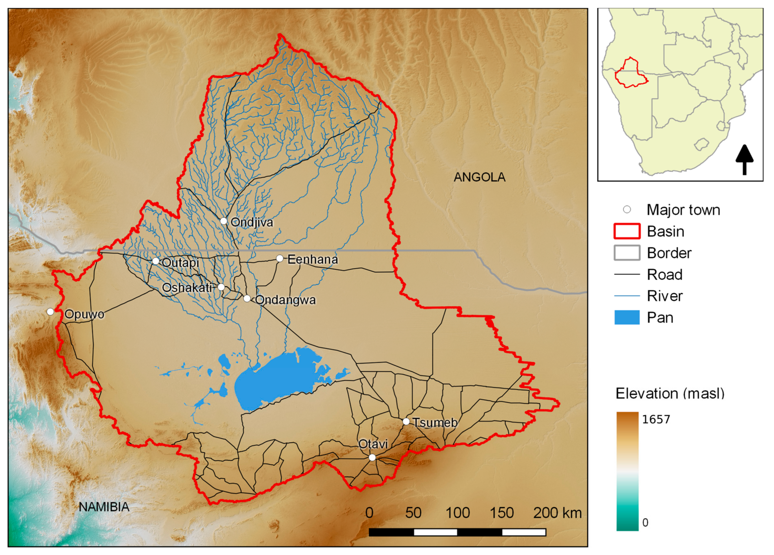
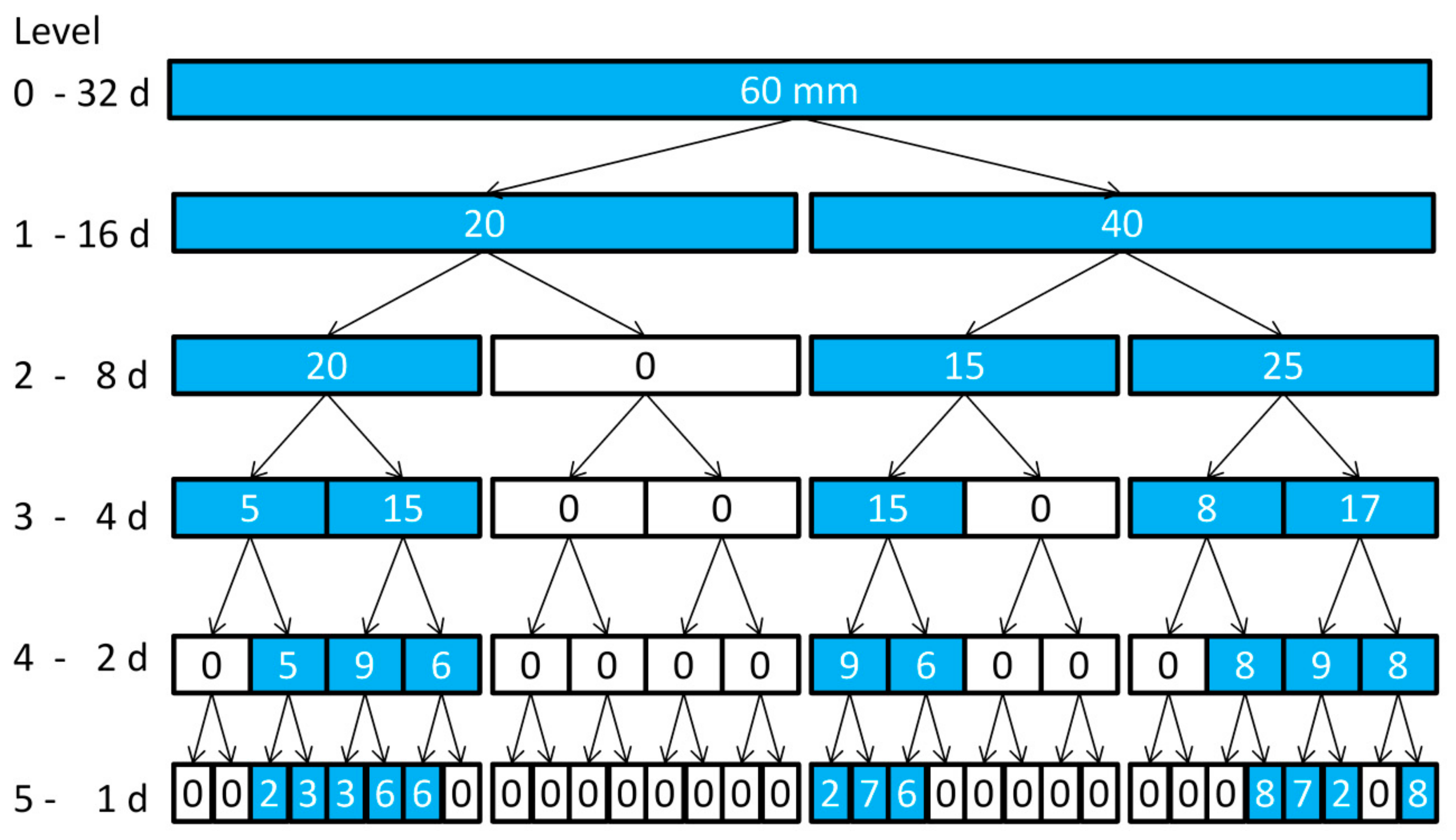
As this study uses the RPs’ estimates for crop model, daily data were obtained for four out of the six products. Only CRU and GPCC are solely available on a monthly basis and, hence, require disaggregation to obtain daily rainfall estimates. Therefore, a multiplicative, micro-canonical cascade model [55] was used for the rainfall disaggregation. The model has been used before for rainfall disaggregation over a wide range of scales, e.g., from monthly to daily values [56], as well as from daily to hourly values [57] and to 5 min values [58] to generate input for rainfall-runoff-modelling [58,59]. The rainfall amount of one time step is divided into b finer time steps of equal length (with b = branching number, see Figure 2 for a schematic illustration). With b = 2 throughout the whole disaggregation process, a daily resolution can only be achieved under the assumption that every month consists of 32 days. Hence, “additional” days in the time series (19 for each year) are removed afterwards on a monthly basis by deleting the first dry day(s) to obtain accurate month lengths. The rainfall amount is conserved exactly during the disaggregation process, so an aggregation of the disaggregated time series would result in the original time series. However, to cover the random behavior of the disaggregation, 80 realizations for each dataset have been created (after 80 realizations the dry spell duration shows only slight changes for the median value as well as maximum and minimum).
The model parameters are estimated from the observed time series at Okatana station. For a more detailed description of the cascade model, the interested reader is referred to [57].
To evaluate the performance of the disaggregation, the observed time series at Okatana station was aggregated from daily to monthly values (32 days) and afterwards disaggregated from monthly to daily values again. This enables comparisons between observed daily values and the disaggregated time series at the same location. The rainfall characteristics for this case show good results in terms of rainfall generation for the number of wet time steps (relative error of −8%), average intensity (9%), and number of dry intervals (1%).
2.4.2. Quantile Mapping
The Quantile Mapping technique adjusts the statistical characteristics of the products’ rainfall estimates (e.g., arithmetic mean, standard deviation) to the observed time series. It corrects the distributions of the RP’s daily precipitation estimates () with the distribution of observed daily precipitation at Okatana station () [60]. The QM technique is mainly applied and evaluated for calibration purposes in global and regional climate models, as well as hydrological contexts [53,61,62,63,64].
The transfer function is used to map the original RP values to the ones of the observed time series, following the equation:
As the distribution of is known, the transformation is carried out as:
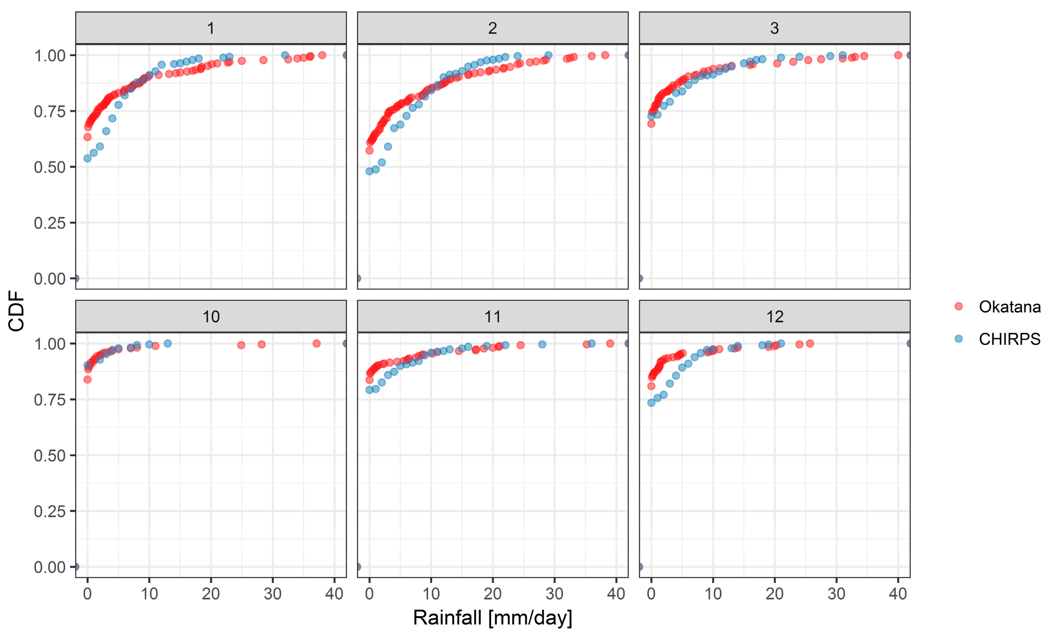
with being the cumulative distribution function (CDF) of and being the inverse CDF of . Instead of relying on parametric distributions, empirical CDFs for the RPs’ time series and Okatana station were used [53,60]. In this regard, the respective CDFs and the corresponding QM parameters were estimated on a monthly basis (Figure 3). This means the available time series at Okatana station from 2001 to 2009 was split into the twelve months from January to December and specific QM parameters were derived for each of the twelve months. The mapping of daily RP values was then performed using the non-parametric transfer functions of the month-specific QM parameters. This ensures a better fit to monthly rainfall characteristics which is particularly relevant in semi-arid environments that show pronounced dry periods.
Overall, the QM procedure was carried out by applying a Monte Carlo cross-validation using 100 model runs for each rainfall product. Each time, the available time series of nine years (2001–2009) was randomly split into seven years for calibration and two years for validation. Based on the mean absolute error (MAE, Equation (5)) between the observed and the RP time series in the validation dataset, the best QM transfer function was identified and applied to the entire product time series. Each of the 80 realizations for CRU and GPCC were also cross-validated using the Monte Carlo technique. The entire procedure was carried out using the ‘qmap’ package [65].
2.4.3. Rainfall Statistics
For the purpose of evaluating the performance of the calibration procedure, the subsequent rainfall statistics were calculated before and after calibration. Alongside the MAE as a standard measure of model performance using the equation [66]:
where is the absolute error term, and other key statistical parameters were evaluated that are relevant for crop modelling in semi-arid environments. In this regard, only the rainy season from October to April was analyzed. First, the mean dry spell duration (days between two rainfall events with at least 1 mm of rainfall) was calculated. Second, the number of rainy days (minimum of 1 mm rainfall) was assessed as annual averages. Third, the daily maximum precipitation was calculated as well as fourth, the mean daily rainfall intensity. Last, the average onset of the rainy season was assessed, using the threshold of at least two days of rain with a minimum of 5 mm.
2.5. Crop Growth Model
The six calibrated, daily RPs and the observed time series at Okatana station are used as input for a crop growth model to assess and analyze the uncertainty between the time series when modelling staple food yields and corresponding nutritional scores in the study area.
The Agricultural Production Systems Simulator (APSIM) [26] model was chosen as an appropriate tool to model millet yield in the Cuvelai-Basin, since it was successfully applied to smallholder systems in semi-arid environments of Sub-Saharan Africa [67,68,69,70]. APSIM is an easy-to-use crop model which offers pre-defined crop configurations that can be adjusted according to data availability. In addition to daily precipitation, the model requires input data of maximum and minimum daily temperature and surface solar radiation. Information on temperature (°C) were derived from the Climate Research Unit dataset (CRU TS3.23) [48] and linearly interpolated from monthly to daily values. Information on daily surface solar radiation (MJ/m2) was derived from monthly cloudiness data from the CRU TS3.23 dataset, as well. The transformation from cloudiness information (% cloud cover) to surface solar radiation was performed using the Supit-van Kappel approach [71], implemented in the R package ‘sirad’ [72] and calibrated with location-specific empirical constants from short-term time series at recently installed meteorological stations from the SASSCAL WeatherNet [73].
As empirical field level data on soil characteristics were not available to the current study, the model’s soil component, in particular the soil water characteristics were configured using the ISRIC World Soil Information Database [74] and information on local field management techniques [75]. The planting date was set to be variable in the window from 1 December to 31 January, based on the threshold of at least 5 mm rainfall within 2 consecutive days.
Table 2 depicts the key soil characteristics that were obtained from the ISRIC database at the location of Okatana station. Empirical pedotransfer functions [76] that are used in the Water Evaluation and Planning Software were applied to calculate soil water characteristics. The air dry conditions were assumed to be 50%, 80%, and 100% of LL15 for the first, second, and deeper soil levels, respectively [77]. Overall, model configuration was kept constant in all model runs, except the precipitation input that was taken from the six RPs and the Okatana time series. As CRU and GPCC were disaggregated from monthly time series, the 80 realizations of each product were processed in APSIM, while the output in yield was averaged.
The yield estimated by the APSIM model was compared to official millet yield data from Central-Northern Namibia for validation. The data is provided by the Agricultural Statistics Bulletin of the Namibian Ministry for Agriculture, Water and Forestry (MAWF) for the period 2000–2009 [36]. Other sources of yield data are available, such as FAOSTAT and the Namibian Agronomic Board. However, the information provided on these platforms is insufficient to determine the origin of the yield data, if it is a national average, measured in northern Namibia or obtained from other parts of the country. The MAWF dataset was then preferred for the validation.
2.6. Nutritional Scores
Characterizing the nutritional situation of individuals or groups, particularly in the context of developing countries, is a major issue of scientific debate. Numerous indicators exist to assess food security conditions or the nutritional status. These include but are not limited to the FAO Indicator of Undernourishment (FAOIU), the Poverty and Hunger Index (PHI), the Diet Diversity Scores (DDS) [78], and the Integrated Food Security Phase Classification (IPC) adopted by the Famine Early Warning System Network (FEWS NET) [79]. The selection of appropriate indicators is important when it comes to the empirical investigation of the effect of agriculture on human nutrition [80]. Recent reviews give an overview of indicator sets used by researchers to empirically assess nutritional status. These indicators cover the areas of anthropometry, biochemistry, diet and food consumption, and food security [15,81,82].
For the purpose of characterizing the nutritional status of households in this study, simple nutritional scores were calculated for dietary energy and the macro-nutrients proteins, lipids and carbohydrates. In this regard, a household’s demand for food was measured against the potential quantities of millet that can be produced in a subsistence farming system of the Cuvelai-Basin. First, the results of the APSIM model runs (kg/ha) are extrapolated to the average farming area per household in the Cuvelai-Basin of about 2.4 ha [83]. The total yield is subsequently transformed into nutritional indicators as referenced in the United States Department of Agriculture (USDA) National Nutrient Database for Standard Reference [84]. Respective values for millet are given in Table 3, based on USDA reference number 20031.
Second, a household’s demand for dietary energy, and particularly for the macronutrients proteins, lipids, and carbohydrates, were estimated to generate a wider picture of human nutrition. Assessments of nutritional status commonly apply nutritional benchmarks to assess the adequacy of food items available to individuals or groups [85]. However, since these benchmarks neglect the importance of physical activity levels as part of the total energy expenditure [86], and only seldom account for other nutritional indicators such as macro-nutrients, this study adopts the concept of dietary reference intakes (DRI) [87]. Herein, the estimated energy requirements (EER) [88] and acceptable macro-nutrient distribution ranges (AMDR) are considered for specific age and gender groups within a certain population. EER benchmarks represent the amount of dietary energy “that is predicted to maintain energy balance in a healthy adult of a defined age, gender, weight, height, and level of physical activity consistent with good health” [87]. To incorporate the important role of macro-nutrients in the provision of dietary energy, group-specific AMDR benchmark values were calculated. “An AMDR is defined as a range of intakes for a particular energy source that is associated with reduced risk of chronic diseases while providing adequate intakes of essential nutrients” [87]. The nutritional benchmarks are represented in Table 3, row 4 based on the assumption of an average household size of 5.5 people and a specific age and gender composition, derived from the last census of Namibia in 2011 [33].
3. Results
This section is divided into four major parts. First, the precarious endowment of the Cuvelai-Basin with reliable rain gauge stations is presented. The second sub-section shows the estimated rainfall of the six products and their specific spatial and temporal characteristics. Therein, calibrated and uncalibrated time series are evaluated against each other. The third sub-section focuses on the results of the APSIM model. The estimated yields are compared to official millet yield data. Fourth, the derived nutritional scores are presented with special emphasis on the fulfilment of a household’s dietary energy demand and its range of uncertainty.
3.1. Local Rain Gauge Measurements
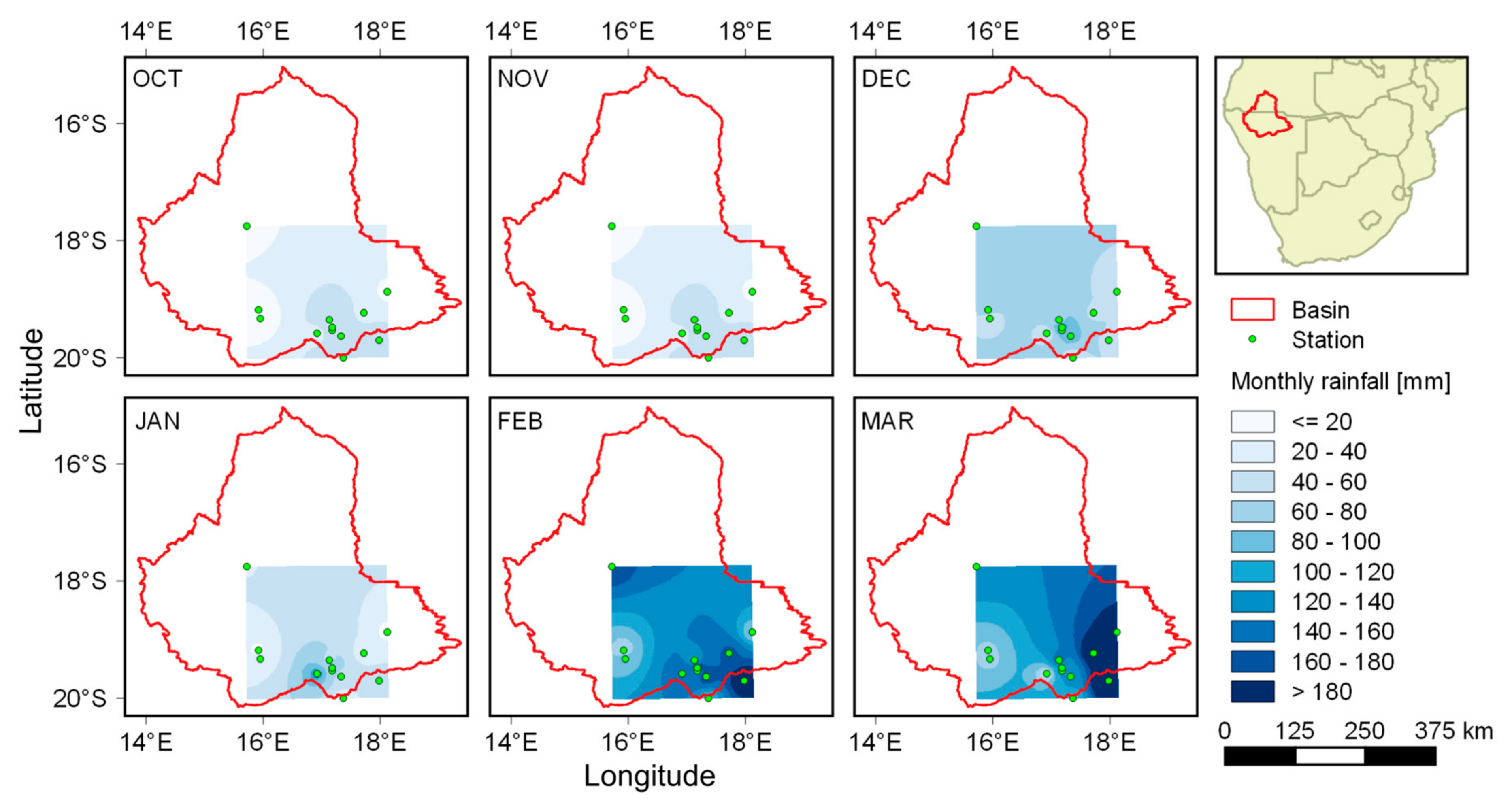
Local rainfall data from gauge stations are available for part of the Cuvelai-Basin [31]. Although the sparsely available rain gauge measurements provide long-term rainfall time series, they do not capture well the spatial rainfall variability in the study area. For clarification of this problem, Figure 4 shows the result of the inverse distance weighting (IDW) interpolation, including stations that—in the period 1980–2009—encompass at least 20 years with complete monthly data records (without any data gaps).
The maps indicate the average rainfall for the months of the rainy season from October to March. Only a fraction of the entire basin can be described with respect to its long-term mean precipitation conditions, as meteorological stations in the north and the west do not provide sufficient data. Even the rectangle in the southeast of the basin is biased, as most stations are located in the south, while only one station provides information on areas further north. Hence, limited opportunities exist to provide a comprehensive picture on average rainfall conditions for the basin that stems solely from rain gauge measurements. For this reason, other options to retrieve rainfall data are outlined in the following sections.
With respect to suitable ground data for RP calibration, daily rainfall data are required. While the stations used for spatial interpolation provide monthly rainfall data for longer periods, they only offer daily data from 1999 to 2010. Table 4 gives an overview of the 12 stations selected, indicating the covered time period, the share of missing values and the longest period available without any data gaps. No station provides a complete daily time series as the share of missing values ranges from 1.5% to 31.9%. Against this background, Okatana station is regarded as the most appropriate time series for RP calibration as it provides the longest daily time series of 3437 days from 1 January 2001 to 31 December 2009 without any missing values.
3.2. Estimated Rainfall
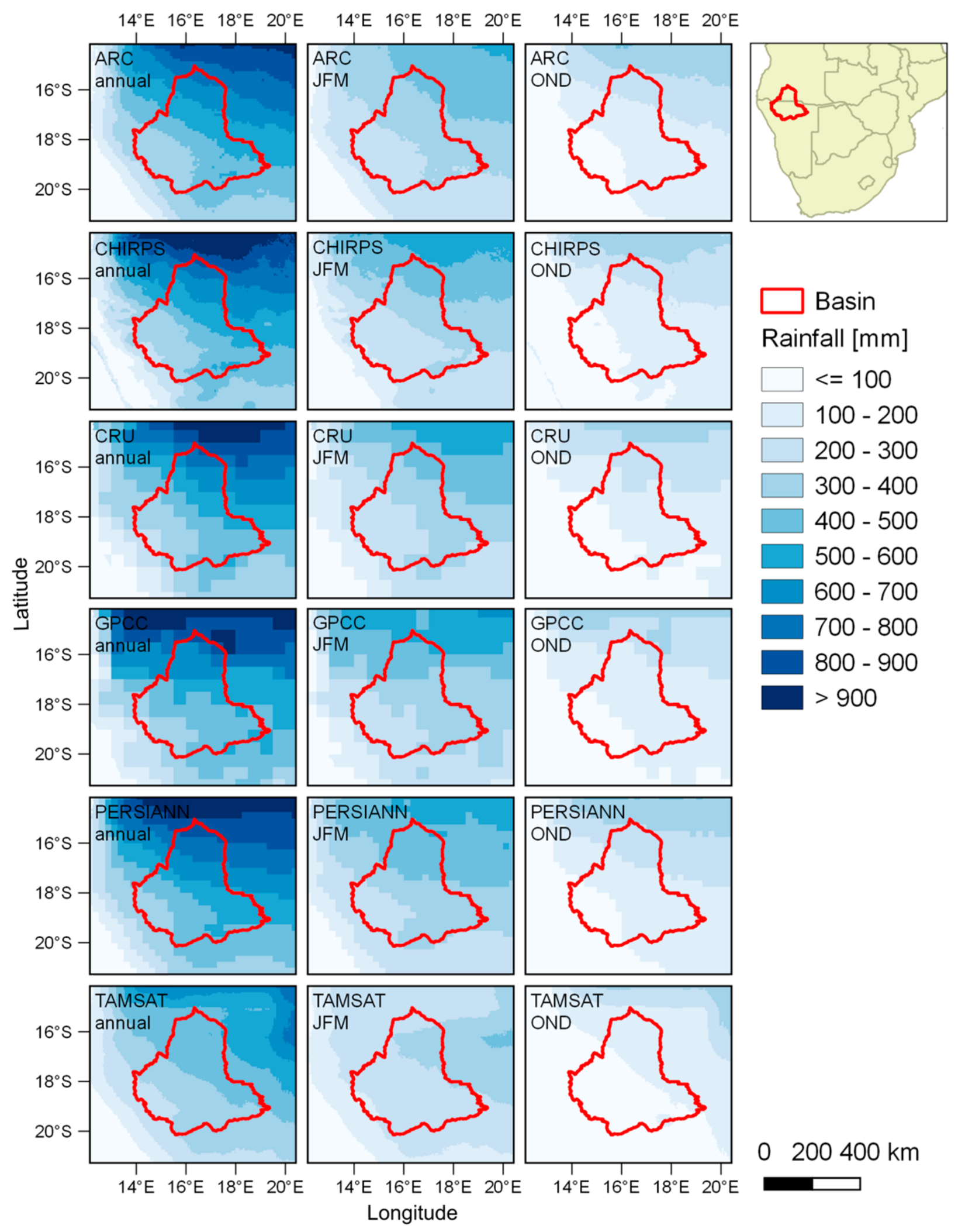
The low quality of available rain gauge measurements necessitates the use of RPs to estimate rainfall conditions for the basin as a whole. Figure 5 presents the uncalibrated annual rainfall as estimated by each of the products. Although the maps show the varying spatial resolution of the products, a consistent spatial pattern is apparent with increasing rainfall from the southwest to the northeast. This spatial pattern, captured by the raster images in Figure 5 with an increasing mean annual rainfall to the northeast, correlates strongly among the products when comparing the raster cell values from one product to another. In this regard, each RP has a Pearson correlation coefficient with every other product of at least r = 0.9. Likewise, considering the basin’s mean annual rainfall as the average raster cell values per year, all RPs show a similar signal over time, with a Pearson coefficient of at least r = 0.73 among the products.
Despite these similarities, differences still exist. The absolute amount of mean annual rainfall differs among the products. Particularly the lowest (TAMSAT, 390 mm) and the highest values (PERSIANN, 544 mm) differ with a range of about 154 mm. Together with CHIRPS, CRU, and GPCC the PERSIANN product estimates higher amounts of rainfall, especially beyond the basin’s boundary in the far north where more than 900 mm are estimated. In comparison to low values of around 200–300 mm per year in the south, this gradient is a key factor of the basin, characterizing the north as rather humid, while the south is semi-arid.
Overall, rainfall occurs during the rainy season between October and May, while the winter months are rather dry. The quarterly plots in Figure 5 show that the fourth quarter (OND) receives less rainfall than the first quarter of a year (JFM). This is particularly relevant for local farmers to decide upon planting which normally starts around December and January, offering the crop favorable water conditions during the growing period in the first months of a year. This quarterly pattern is well reproduced again by all RPs, with TAMSAT being the one with the lowest absolute estimates.
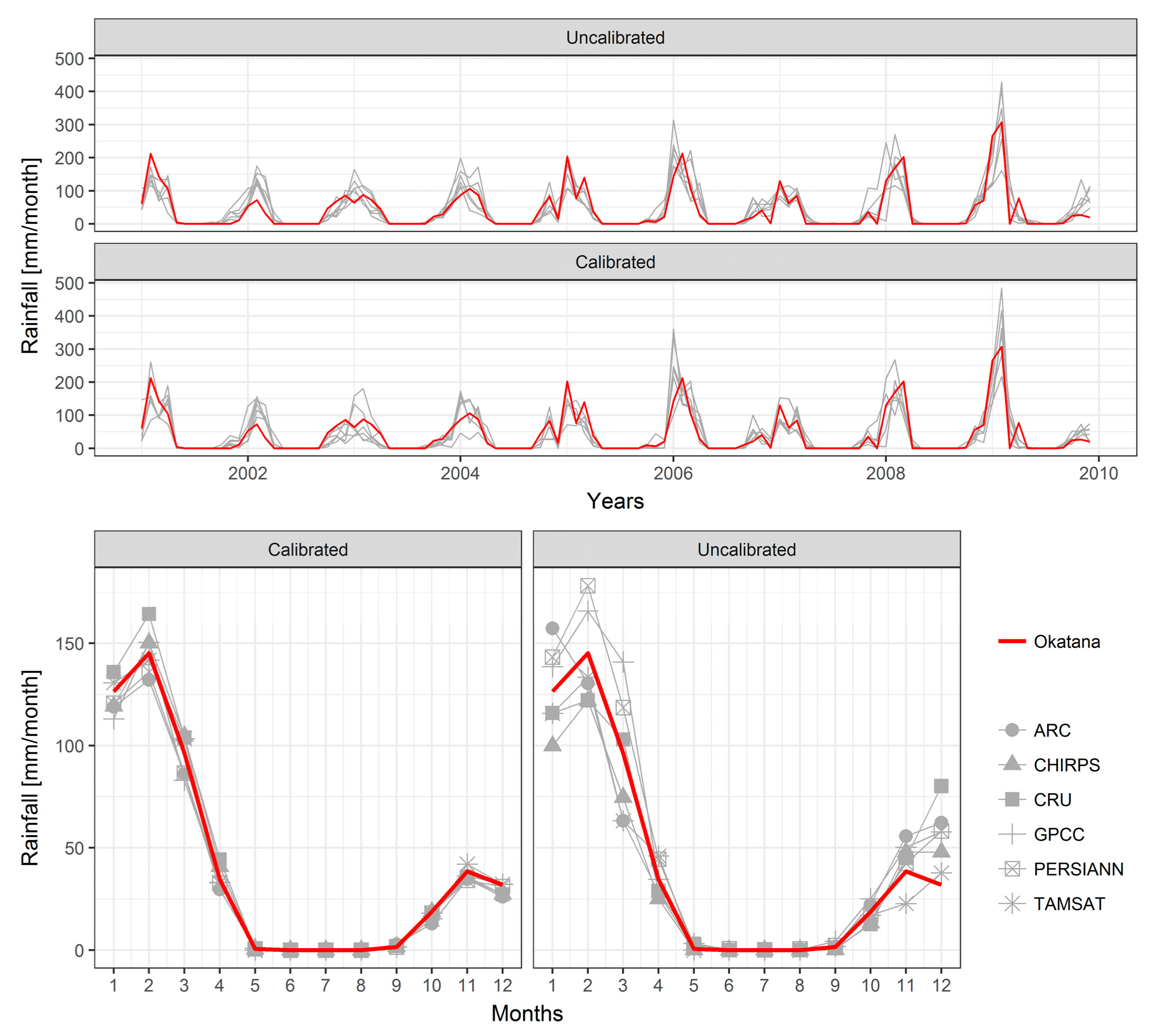
The RPs presented above are calibrated to the observed rainfall time series from Okatana station in Central-Northern Namibia. Prior to this, the CRU and GPCC products were disaggregated from the monthly to the daily scale. Afterwards, they were treated in the same way as the other RPs. The QM calibration technique aligns key rainfall characteristics to the observed time series.
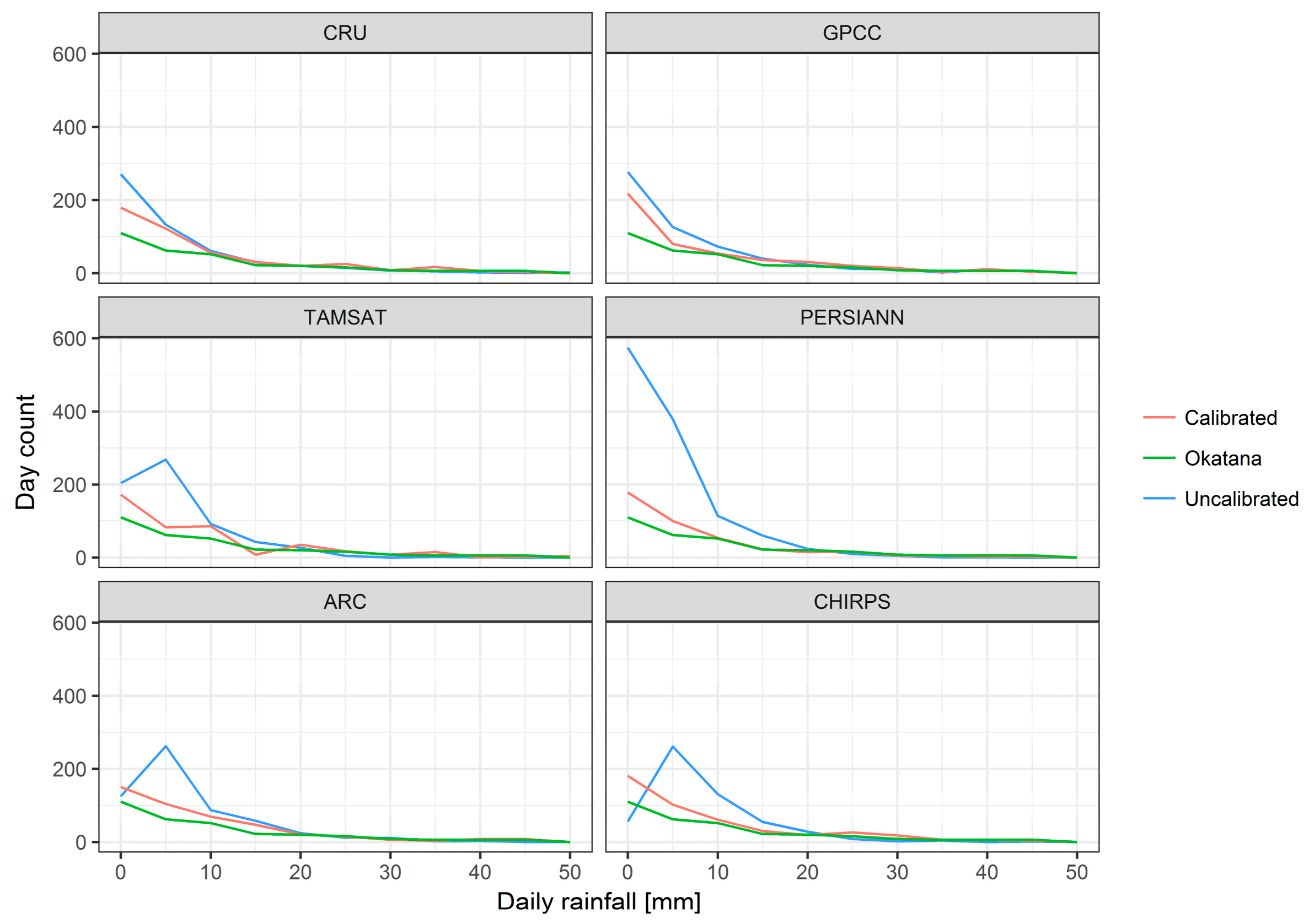
Figure 6 presents the results of the calibration procedure. The plots on the left hand-side show the uncalibrated and calibrated monthly rainfall at Okatana station, estimated by the RPs at the specific pixel location. Overall, the seasonality of the basin’s climate becomes obvious with peak rainy seasons recorded in the years 2006, 2008, and 2009. The RPs reproduce well the Okatana time series signal with an average Pearson correlation coefficient of r = 0.84. The plots on the right present the monthly precipitation, averaged over the available nine years. In particular, the months January, February, and March, as well as November and December, show deviations among the products before calibration. After the QM procedure, all deviations in the monthly average values were reduced and aligned to the Okatana time series (lower right plot). Exemplarily, the MAE between the observed and the estimated monthly averages is reduced from 6.20 to 2.94 mm. Nevertheless, a perfect fit cannot be obtained, as the selection of the best transfer functions is based on the QM model’s performance in the validation dataset. Hence, not all data of the available nine years serve to parameterize the transfer functions resulting in persisting residuals. Since the month of February still shows the largest deviations after calibration, Figure 7 presents the frequency distributions of the month’s daily rainfall. All products improve, as the frequency distributions are better aligned to the observed one. As observable in Figure 6, in particular the PERSIANN product overestimates the frequency of small rainfall events (<10 mm/day) before calibration.
The rainfall statistics confirm a better fit to Okatana station data. Table 5 presents key rainfall characteristics, comparing the uncalibrated and calibrated RP time series to the observed one from Okatana station between the years 2001 and 2009. Overall, the QM calibration procedure improves most of the statistics, compared to the raw data. This is particularly true for the number of rainy days and the rainfall intensities that improve for all RPs. Only the fit of the ARC product in terms of the dry spell duration and average daily rainfall slightly decreases. The latter is also true for the GPCC product. With regard to the MAE, the CHIRPS and TAMSAT, as well as CRU products, slightly decrease in performance, while all other products are enhanced.
3.3. Estimated Yield
Having presented the rainfall results in the previous sections, the following ones now focus on the estimated millet yield from the APSIM model runs. Therein, the six RPs were used as model input and compared to official millet yield data. It has to be noted that the 80 disaggregated and calibrated time series from CRU and GPCC were all processed in the APSIM model. The results were averaged (median) over all model runs to obtain a final, product-specific result.
Figure 8 compares the APSIM model results that use the uncalibrated (upper plot) and the calibrated rainfall estimates (lower plot). Despite the deviations in absolute yield, the crop model performs well in estimating the extraordinary low yields from subsistence agriculture in Northern Namibia [35]. Nevertheless, the median values of the calibrated products range between 264.74 kg/ha (CRU) and 363.08 kg/ha (CHIRPS) compared to 208.88 kg/ha, as officially recorded. In comparison to the modelled yield that used the uncalibrated products, the results of the calibrated ones show smaller distribution ranges and fewer failed harvest events. Overall, these results fit better to the model results that make use of the observed rainfall time series from Okatana station. While most products score above 300 kg/ha, the CRU and GPCC products score below this threshold. This is primarily triggered by the fact that some of the 80 APSIM model runs failed and produced no harvestable yield, resulting in a decreased overall product performance.
In terms of temporal consistency, the reader is referred to Figure 9 in the following sub-section that depicts the yield results in terms of nutritional coverage ratios. Against the background of the study’s design in which no crop model calibration could be performed with on-site data, the APSIM model configuration can be regarded as suitable, since the modelled yield that uses rainfall data from Okatana station shows a moderate correlation with the official data (r = 0.52). With regard to the calibrated products, the modelled yields only achieve Pearson correlation coefficients of up to 0.18 (CHIRPS). The official yield time series largely scores below the RPs and shows a higher inter-annual fluctuation (Figure 9). This fluctuation can be explained by drought and flood events that had an impact on agricultural production. While the years 1995, 2003, and 2013 are known as drought years [32], the years 2008 and 2009 were recorded as flood years and, hence, potentially caused reduced yields [35]. In these flood years, however, the precipitation conditions would have made higher yields possible as indicated by the RPs’ results. In particular, the adverse impact from flood events is not captured in the crop model and may explain part of the deviations between modelled and officially-observed yields.
3.4. Nutritional Scores
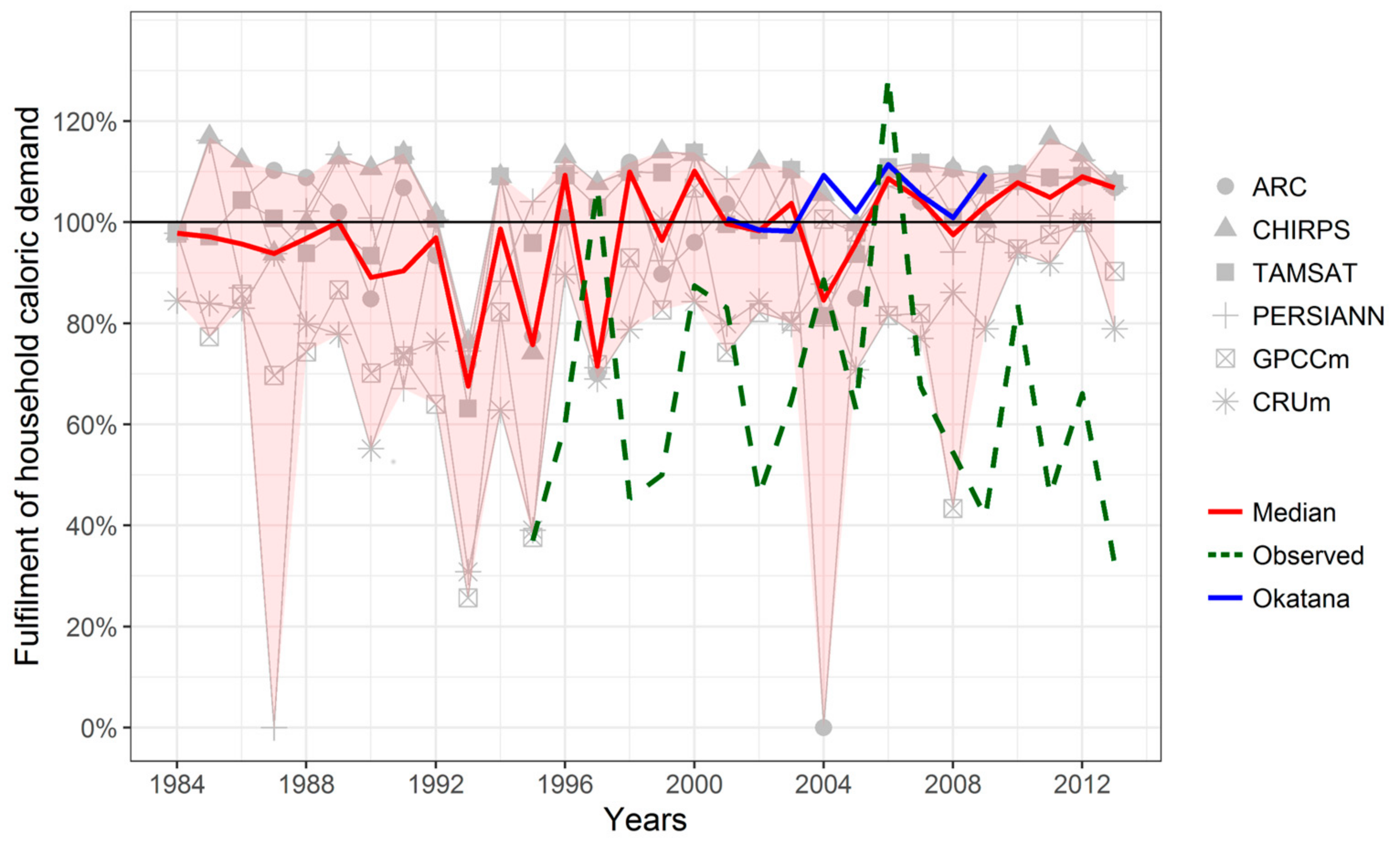
The estimated yields from the APSIM model runs were transformed into nutritional supply indicators for dietary energy, proteins, lipids, and carbohydrates. These indicators were measured against the nutritional demand of a typical Cuvelai household to obtain nutritional scores. Figure 9 shows the degree of fulfilment of a household’s dietary energy demand over time from 1984 to 2013. The red line represents the median degree of fulfilment by considering all model runs, while the light red area indicates the domain of uncertainty, generated by the model results of the individual RPs. The specific nutritional scores estimated by the products are depicted in light grey. For the purpose of comparison, the green line indicates the degree of fulfilment based on the observed data of millet yield from Central-Northern Namibia (1995–2013).
It becomes obvious that the degree of fulfilment fluctuates around the total fulfilment of the dietary energy demand with an average of 97%. However, differences are apparent for a range of years. In this regard, Figure 9 shows large differences in 1987 and 2004. In these years, the PERSIANN and ARC products fail in generating yield as limited soil moisture prevents the crop from germinating. Both products show longer dry spell durations and fewer rainy days compared to the observed data (Table 4) which might be an explanation for model failure in specific years. The year 1993 stands out in which all products point to low yield and, hence, a critical energy demand fulfilment of only 68% (median). This year is well known to be a severe drought year, particularly affecting the agricultural production of the northern regions [32,89]. The remaining years show heterogeneous RP signals, while the median stays rather constant around 90–100% of fulfilment. The same temporal signal is valid for the other macro-nutrient indicators. Based on the nutrient content of the millet plant, however, the mean degree of fulfilment of a household’s protein, lipid, and carbohydrate demand differs from the dietary energy demand (114%, 49%, and 167%, respectively).
4. Discussion
The interpolation of available rainfall data from gauge stations in the Cuvelai-Basin uncovered a deficit in the spatial endowment with meteorological stations. The Angolan part of the basin is poorly equipped, while the Namibian side manifests better coverage. Anyhow, the last years showed an improvement of the data situation. Despite this progress, no reliable estimate on current and past rainfall can be obtained from the station network for the basin as a whole. The use of RPs is, therefore, necessary to perform a range of applications in the field of hydrological and agricultural modelling.
The disaggregation technique applied in this study to obtain daily rainfall estimates from monthly aggregates proved to be a promising opportunity for application in agricultural modelling. Though it was predominantly used on smaller time scales before (disaggregation of daily data) and requires a higher computational effort (in this study, 80 realizations were generated for CRU and GPCC products, each), the disaggregated daily rainfall estimates were largely able to reproduce the characteristics of the observed time series. This is particularly true when considering the final rainfall time series after the calibration procedure. The quantile mapping calibration technique, offers a feasible solution to obtain rainfall estimates that are aligned to key statistics of observed time series. Especially, parameters such as dry spell duration, rainy day count, and onset of the rainy season, are important determinants for crop model applications that can be improved using the QM methodology.
Nonetheless, the RPs still show differences, notably in terms of absolute rainfall on daily, monthly, and annual levels. These differences stem from multiple influencing factors, such as sensor types, processing algorithms, and spatial resolutions. As in the case of the ARC product, the fixed rainfall rate of 3 mm·h−1 might only be the correct correlation between cloud cover duration and precipitation at some locations. While it proves very accurate for the Sahel zone [90], and satisfactory for some locations in Central Africa [91], it underestimates precipitation in comparison to station data in Eastern Africa [92] and in rain shadows [91]. Likewise, the other products build on certain assumptions that might not perfectly fit the conditions of a particular study site. Hence, the calibration of RPs with locally-observed rainfall data is a prerequisite. Furthermore, research into the suitability of other RPs, such as CMORPH [93] and MSWEP [94] that are also used for studies in Africa, constitute valuable prospects for further analyses.
The different rainfall signals have an impact on subsequent modelling stages, as shown in the exemplary APSIM crop model. Though the modelled yield does not entirely reproduce the observed data, the results are reasonable first estimates for the nutritional situation in the Cuvelai-Basin. However, the quality and reliability of the official time series on millet yield must also be regarded as questionable as auxiliary information on how the data was assessed (e.g., location, timing, and sampling) is not available. Overall, this study fell back on auxiliary information from a literature survey and a large-scale soil property dataset to configure the crop model. Model performance can be enhanced by calibrating the model with locally-collected data on soil water and plant growth characteristics, and with management practices in terms of plant density, planting depth, and date of planting. In conjunction with the consideration of third variables such as the effect of flooding, model performance can potentially be enhanced.
All in all, the results provide insights into the nutritional situation of a typical household in the Cuvelai-Basin from a remote sensing perspective. Recent food consumption assessments show that subsistence grain farming is not necessarily capable of constantly fulfilling a household’s nutritional demand [95]. This is confirmed by the official and the modelled yield results, both of which manifest a fluctuating fulfilment of demand. Although the dietary energy demand of a typical Cuvelai household is almost met on average, the provision of lipids is not sufficient. Here, other food sources, such as animal products, vegetables, and purchased groceries, complement the diet obtained from subsistence farming.
5. Conclusions
This study explores the uncertainty among six rainfall products in the Cuvelai-Basin. It compares the rainfall estimates to locally-observed time series and performs quantile mapping to calibrate key rainfall characteristics. As a result, the RPs correlate well with the observed rainfall (r = 0.84) and better reproduce dry spell durations, rainy day counts, and rainfall intensities. Nevertheless, the persisting differences among the products percolate through the exemplary crop model into the final results of millet yield and associated nutritional scores. The crop model reproduces the extraordinary low yields from the study area and, in particular, the temporal fluctuation of the observed yield when ground data on rainfall from Okatana station are processed (r = 0.52). The individual products’ performances, however, are rather heterogeneous with CHIRPS performing best to capture the temporal yield signal (r = 0.18). Translated into the fulfilment of a household’s dietary energy demand, 97% can be met on average. Nevertheless, high annual fluctuations are apparent due to input data uncertainty. Overall, this study makes contributions to the field of rainfall data analysis, agricultural modelling, and food security monitoring.
First, it shows that rainfall products entail uncertainties due to differences in sensor techniques, processing algorithms, and spatial and temporal coverage and resolution. These have to be taken into account when RPs are used for further processing. Since in situ measurements of rainfall are scarce in large areas of SSA, modelers need to fall back on rainfall products to perform their calculations. In these cases, the selection of an appropriate rainfall product must be made explicit, since multiple options exist, all leading to different results. Thus, in the absence of observed data with which to identify the most accurate RP, precedence should be given to a multi-model approach to account for inter-product uncertainty.
Second, crop models that are driven by high-resolution rainfall data and auxiliary information provide promising opportunities for the identification of food insecurity hot spots. The results presented in this study can be made spatially explicit by incorporating census information on household characteristics, such as household size and composition, farming area, and agricultural activities. Applying seasonal rainfall forecasts to the model may help to improve early warning capabilities, against the background of the minor role crop models play in the current configuration of famine early warning systems [1]. Reducing data input uncertainty improves the accuracy of current models and consequently advances the precision of predictions for the future.
Third, the coverage of rain gauge stations in Sub-Saharan Africa is insufficient for a range of modelling and monitoring purposes. Hence, prompt extension of the current station network is required to improve short and long-term capacities for tackling food security challenges.
Acknowledgments
This study was funded by the German Federal Ministry of Education and Research (BMBF) as part of the ‘Southern African Science Service Centre for Climate Change and Adaptive Land Management’ (SASSCAL) (task 016, grant no. 01LG1201I).
Author Contributions
Robert Luetkemeier and Stefan Liehr conceived and designed the study; Robert Luetkemeier, Lina Stein, and Lukas Drees processed the rainfall data; Hannes Müller conducted the rainfall disaggregation; Robert Luetkemeier carried out the rainfall data calibration, crop model application and evaluation; Robert Luetkemeier wrote the paper; and the co-authors contributed text blocks.
Conflicts of Interest
The authors declare no conflict of interest. The founding sponsors had no role in the design of the study; in the collection, analyses, or interpretation of data; in the writing of the manuscript, and in the decision to publish the results.
References
- Brown, M.E.; Brickley, E.B. Evaluating the use of remote sensing data in the U.S. Agency for International Development Famine Early Warning Systems Network. J. Appl. Remote Sens. 2012, 6, 063511. [Google Scholar] [CrossRef]
- McMillan, H.; Jackson, B.; Clark, M.; Kavetski, D.; Woods, R. Rainfall uncertainty in hydrological modelling: An evaluation of multiplicative error models. J. Hydrol. 2011, 400, 83–94. [Google Scholar] [CrossRef]
- WMO. Status of the Global Observing System for Climate; World Meteorological Organization (WMO): Geneva, Switzerland, 2015. [Google Scholar]
- Liu, G. Satellites and satellite remote sensing. Precipitation. In Encyclopedia of Atmospheric Sciences, 2nd ed.; Pyle, J., Zhang, F., Eds.; Academic Press: Oxford, UK, 2015; pp. 107–115. ISBN 978-0-12-382225-3. [Google Scholar]
- Yuter, S.E. RADAR | Precipitation Radar. In Encyclopedia of Atmospheric Sciences, 2nd ed.; Pyle, J., Zhang, F., Eds.; Academic Press: Oxford, UK, 2015; pp. 455–469. ISBN 978-0-12-382225-3. [Google Scholar]
- AghaKouchak, A.; Mehran, A.; Norouzi, H.; Behrangi, A. Systematic and random error components in satellite precipitation data sets. Geophys. Res. Lett. 2012, 39, L09406. [Google Scholar] [CrossRef]
- Moazami, S.; Golian, S.; Kavianpour, M.R.; Hong, Y. Uncertainty analysis of bias from satellite rainfall estimates using copula method. Atmos. Res. 2014, 137, 145–166. [Google Scholar] [CrossRef]
- Skinner, C.J.; Bellerby, T.J.; Greatrex, H.; Grimes, D.I.F. Hydrological modelling using ensemble satellite rainfall estimates in a sparsely gauged river basin: The need for whole-ensemble calibration. J. Hydrol. 2015, 522, 110–122. [Google Scholar] [CrossRef]
- Pessacg, N.; Flaherty, S.; Brandizi, L.; Solman, S.; Pascual, M. Getting water right: A case study in water yield modelling based on precipitation data. Sci. Total Environ. 2015, 537, 225–234. [Google Scholar] [CrossRef] [PubMed]
- Hughes, D.A. Comparison of satellite rainfall data with observations from gauging station networks. J. Hydrol. 2006, 327, 399–410. [Google Scholar] [CrossRef]
- Thornton, P.K.; Bowen, W.T.; Ravelo, A.C.; Wilkens, P.W.; Farmer, G.; Brock, J.; Brink, J.E. Estimating millet production for famine early warning: An application of crop simulation modelling using satellite and ground-based data in Burkina Faso. Agric. For. Meteorol. 1997, 83, 95–112. [Google Scholar] [CrossRef]
- Ramarohetra, J.; Sultan, B.; Baron, C.; Gaiser, T.; Gosset, M. How satellite rainfall estimate errors may impact rainfed cereal yield simulation in West Africa. Agric. For. Meteorol. 2013, 180, 118–131. [Google Scholar] [CrossRef]
- Yuan, W.; Chen, Y.; Xia, J.; Dong, W.; Magliulo, V.; Moors, E.; Olesen, J.E.; Zhang, H. Estimating crop yield using a satellite-based light use efficiency model. Ecol. Indic. 2016, 60, 702–709. [Google Scholar] [CrossRef]
- Roca, R.; Chambon, P.; Jobard, I.; Kirstetter, P.-E.; Gosset, M.; Berges, J.C. Comparing Satellite and Surface Rainfall Products over West Africa at Meteorologically Relevant Scales during the AMMA Campaign Using Error Estimates. J. Appl. Meteorol. Climatol. 2010, 49, 715–731. [Google Scholar] [CrossRef]
- Herforth, A.; Ballard, T.J. Nutrition indicators in agriculture projects: Current measurement, priorities, and gaps. Glob. Food Secur. 2016, 10, 1–10. [Google Scholar] [CrossRef]
- Thornton, P.K.; Herrero, M. Adapting to climate change in the mixed crop and livestock farming systems in sub-Saharan Africa. Nat. Clim. Chang. 2015, 5, 830–836. [Google Scholar] [CrossRef]
- Diao, X.; Hazell, P.; Thurlow, J. The Role of Agriculture in African Development. World Dev. 2010, 38, 1375–1383. [Google Scholar] [CrossRef]
- Shiferaw, B.; Tesfaye, K.; Kassie, M.; Abate, T.; Prasanna, B.M.; Menkir, A. Managing vulnerability to drought and enhancing livelihood resilience in sub-Saharan Africa: Technological, institutional and policy options. Weather Clim. Extremes 2014, 3, 67–79. [Google Scholar] [CrossRef]
- Collier, P.; Dercon, S. African Agriculture in 50 Years: Smallholders in a Rapidly Changing World? World Dev. 2014, 63, 92–101. [Google Scholar] [CrossRef]
- FAOSTAT. FAOSTAT. Available online: http://faostat3.fao.org/browse/O/*/E (accessed on 18 July 2016).
- Cooper, P.J.M.; Dimes, J.; Rao, K.P.C.; Shapiro, B.; Shiferaw, B.; Twomlow, S. Coping better with current climatic variability in the rain-fed farming systems of sub-Saharan Africa: An essential first step in adapting to future climate change? Agric. Ecosyst. Environ. 2008, 126, 24–35. [Google Scholar] [CrossRef] [Green Version]
- United Nations (UN). The Millennium Development Goals Report 2015; United Nations (UN): New York, NY, USA, 2015. [Google Scholar]
- UNECA; AU; ADB; UNDP. MDG Report 2015. Lessons Learned in Implementing the MDGs. Assessing Progress in Africa toward the Millennium Development Goals; United Nations Economic Commission for Africa (UNECA); African Union; African Development Bank; United Nations Development Programme (UNDP): Addis Ababa, Ethiopia, 2015; ISBN 978-99944-61-73-8. [Google Scholar]
- Gautam, M. Managing Drought in Sub-Saharan Africa: Policy Perspectives; The World Bank: Washington, DC, USA, 2006. [Google Scholar]
- Von Uexkull, N. Sustained drought, vulnerability and civil conflict in Sub-Saharan Africa. Political Geogr. 2014, 43, 16–26. [Google Scholar] [CrossRef]
- Holzworth, D.P.; Huth, N.I.; deVoil, P.G.; Zurcher, E.J.; Herrmann, N.I.; McLean, G.; Chenu, K.; van Oosterom, E.J.; Snow, V.; Murphy, C.; et al. APSIM—Evolution towards a new generation of agricultural systems simulation. Environ. Model. Softw. 2014, 62, 327–350. [Google Scholar] [CrossRef]
- Mendelsohn, J.; Jarvis, A.; Robertson, T. A Profile and Atlas of the Cuvelai-Etosha Basin; Research and Information Services of Namibia (RAISON) & Gondwana Collection: Windhoek, Namibia, 2013; ISBN 978-99916-780-7-8. [Google Scholar]
- Geofabrik OpenStreetMap Dataset on Angolan Infrastructure. Available online: http://download.geofabrik.de/africa/angola-latest-free.shp.zip (accessed on 18 December 2017).
- Geofabrik OpenStreetMap Dataset on Namibian Infrastructure. Available online: http://download.geofabrik.de/africa/namibia-latest-free.shp.zip (accessed on 18 December 2017).
- Jarvis, A.; Reuter, H.I.; Nelson, A.; Guevara, E. Hole-Filled Seamless SRTM Data for the Globe Version4. Available online: http://srtm.csi.cgiar.org/ (accessed on 16 August 2016).
- Namibian Meteorological Service. Precipitation data for central-northern Namibia 2013. (unpublished).
- EM-DAT. International Disaster Database (EM-DAT), Centre for Research on the Epidemiology of Disasters (CRED). Available online: http://www.emdat.be/advanced_search/index.html (accessed on 26 July 2016).
- NSA. Namibia 2011. Population & Housing Census Main Report; Namibia Statistics Agency (NSA): Windhoek, Namibia, 2013; p. 214. [Google Scholar]
- INE. Resultados Definitivos do Recenseamento Geral da Populacao e da Habitacao de Angola 2014; Instituto Nacional de Estatistica (INE): Luanda, Angola, 2016; p. 213. [Google Scholar]
- Andreas, J. Trends of pearl millet (Pennisetum glaucum) yields under climate variability conditions in Oshana Region, Namibia. Int. J. Ecol. Ecosolution 2015, 2, 49–62. [Google Scholar]
- MAWF. Agricultural Statistics Bulletin; Ministry of Agriculture, Water and Forestry (MAWF): Windhoek, Namibia, 2011.
- Luetkemeier, R.; Liehr, S. Impact of drought on the inhabitants of the Cuvelai watershed: A qualitative exploration. In Drought: Research and Science-Policy Interfacing; Alvarez, J., Solera, A., Paredes-Arquiola, J., Haro-Monteagudo, D., van Lanen, H., Eds.; CRC Press: Leiden, The Netherlands, 2015; pp. 41–48. ISBN 978-1-138-02779-4. [Google Scholar]
- Hoffmann, M.; Schwartengräber, R.; Wessolek, G.; Peters, A. Comparison of simple rain gauge measurements with precision lysimeter data. Atmos. Res. 2016, 174–175, 120–123. [Google Scholar] [CrossRef]
- Di Piazza, A.; Conti, F.L.; Noto, L.V.; Viola, F.; La Loggia, G. Comparative analysis of different techniques for spatial interpolation of rainfall data to create a serially complete monthly time series of precipitation for Sicily, Italy. Int. J. Appl. Earth Obs. Geoinf. 2011, 13, 396–408. [Google Scholar] [CrossRef]
- Unruh, J.D. Eviction policy in postwar Angola. Land Use Policy 2012, 29, 661–663. [Google Scholar] [CrossRef]
- Kaspar, F.; Helmschrot, J.; Mhanda, A.; Butale, M.; de Clercq, W.; Kanyanga, J.K.; Neto, F.O.S.; Kruger, S.; Castro Matsheka, M.; Muche, G.; et al. The SASSCAL contribution to climate observation, climate data management and data rescue in Southern Africa. Adv. Sci. Res. 2015, 12, 171–177. [Google Scholar] [CrossRef] [Green Version]
- Wagner, P.D.; Fiener, P.; Wilken, F.; Kumar, S.; Schneider, K. Comparison and evaluation of spatial interpolation schemes for daily rainfall in data scarce regions. J. Hydrol. 2012, 464–465, 388–400. [Google Scholar] [CrossRef]
- Project QGIS User Guide Release 2.8 2016. Available online: http://www.qgis.org/en/docs/index.html (accessed on 4 May 2016).
- Hijmans, R.J.; van Etten, J.; Cheng, J.; Mattiuzzi, M.; Summer, M.; Greenberg, J.A.; Lamigueiro, O.P.; Bevan, A.; Racine, E.B.; Shortridge, A. Package “raster”, version 2.5-2. Available online: https://cran.r-project.org/web/packages/raster/raster.pdf (accessed on 4 May 2016).
- Funk, C.; Peterson, P.; Landsfeld, M.; Pedreros, D.; Verdin, J.; Shukla, S.; Husak, G.; Rowland, J.; Harrison, L.; Hoell, A.; et al. The climate hazards infrared precipitation with stations—A new environmental record for monitoring extremes. Sci. Data 2015, 2, 150066. [Google Scholar] [CrossRef] [PubMed]
- Schneider, U.; Becker, A.; Finger, P.; Meyer-Christoffer, A.; Rudolf, B.; Ziese, M. GPCC Full Data Reanalysis Version 7.0 at 0.5°: Monthly Land-Surface Precipitation from Rain-Gauges built on GTS-based and Historic Data. Sci. Tech. Data 2015. [Google Scholar] [CrossRef]
- Novella, N.S.; Thiaw, W.M. African Rainfall Climatology Version 2 for Famine Early Warning Systems. J. Appl. Meteorol. Climatol. 2012, 52, 588–606. [Google Scholar] [CrossRef]
- Harris, I.; Jones, P.D.; Osborn, T.J.; Lister, D.H. Updated high-resolution grids of monthly climatic observations—The CRU TS3.10 Dataset. Int. J. Climatol. 2014, 34, 623–642. [Google Scholar] [CrossRef] [Green Version]
- Tarnavsky, E.; Grimes, D.; Maidment, R.; Black, E.; Allan, R.P.; Stringer, M.; Chadwick, R.; Kayitakire, F. Extension of the TAMSAT Satellite-Based Rainfall Monitoring over Africa and from 1983 to Present. J. Appl. Meteorol. Climatol. 2014, 53, 2805–2822. [Google Scholar] [CrossRef]
- Ashouri, H.; Hsu, K.-L.; Sorooshian, S.; Braithwaite, D.K.; Knapp, K.R.; Cecil, L.D.; Nelson, B.R.; Prat, O.P. PERSIANN-CDR: Daily Precipitation Climate Data Record from Multisatellite Observations for Hydrological and Climate Studies. Bull. Am. Meteorol. Soc. 2014, 96, 69–83. [Google Scholar] [CrossRef]
- Maidment, R.I.; Grimes, D.; Allan, R.P.; Tarnavsky, E.; Stringer, M.; Hewison, T.; Roebeling, R.; Black, E. The 30 year TAMSAT African Rainfall Climatology and Time series (TARCAT) data set. J. Geophys. Res. Atmos. 2014, 119, 2014JD021927. [Google Scholar] [CrossRef]
- Funk, C.C.; Peterson, P.J.; Landsfeld, M.F.; Pedreros, D.H.; Verdin, J.P.; Rowland, J.D.; Romero, B.E.; Husak, G.J.; Michaelsen, J.C.; Verdin, A.P. A Quasi-Global Precipitation Time Series for Drought Monitoring; Data Series; U.S. Geological Survey: Reston, VA, USA, 2014; p. 12.
- Ringard, J.; Seyler, F.; Linguet, L. A Quantile Mapping Bias Correction Method Based on Hydroclimatic Classification of the Guiana Shield. Sensors 2017, 17, 1413. [Google Scholar] [CrossRef] [PubMed]
- Wood, S.J.; Jones, D.A.; Moore, R.J. Static and dynamic calibration of radar data for hydrological use. Hydrol. Earth Syst. Sci. 2001, 4, 545–554. [Google Scholar] [CrossRef]
- Olsson, J. Evaluation of a scaling cascade model for temporal rain- fall disaggregation. Hydrol. Earth Syst. Sci. 1998, 2, 19–30. [Google Scholar] [CrossRef]
- Thober, S.; Mai, J.; Zink, M.; Samaniego, L. Stochastic temporal disaggregation of monthly precipitation for regional gridded data sets. Water Resour. Res. 2014, 50, 8714–8735. [Google Scholar] [CrossRef]
- Müller, H.; Haberlandt, U. Temporal Rainfall Disaggregation with a Cascade Model: From Single-Station Disaggregation to Spatial Rainfall. J. Hydrol. Eng. 2015, 20, 04015026. [Google Scholar] [CrossRef]
- Müller, H.; Haberlandt, U. Temporal rainfall disaggregation using a multiplicative cascade model for spatial application in urban hydrology. J. Hydrol. 2018, 556, 847–864. [Google Scholar] [CrossRef]
- Ding, J.; Wallner, M.; Müller, H.; Haberlandt, U. Estimation of instantaneous peak flows from maximum mean daily flows using the HBV hydrological model. Hydrol. Process. 2016, 30, 1431–1448. [Google Scholar] [CrossRef]
- Gudmundsson, L.; Bremnes, J.B.; Haugen, J.E.; Engen-Skaugen, T. Technical Note: Downscaling RCM precipitation to the station scale using statistical transformations & ndash; a comparison of methods. Hydrol. Earth Syst. Sci. 2012, 16, 3383–3390. [Google Scholar] [CrossRef]
- Cannon, A.J. Multivariate quantile mapping bias correction: An N-dimensional probability density function transform for climate model simulations of multiple variables. Clim. Dyn. 2017, 50, 31–49. [Google Scholar] [CrossRef]
- Ehret, U.; Zehe, E.; Wulfmeyer, V.; Warrach-Sagi, K.; Liebert, J. Should we apply bias correction to global and regional climate model data? Hydrol. Earth Syst. Sci. 2012, 16, 3391–3404. [Google Scholar] [CrossRef]
- Muerth, M.J.; Gauvin St-Denis, B.; Ricard, S.; Velázquez, J.A.; Schmid, J.; Minville, M.; Caya, D.; Chaumont, D.; Ludwig, R.; Turcotte, R. On the need for bias correction in regional climate scenarios to assess climate change impacts on river runoff. Hydrol. Earth Syst. Sci. 2013, 17, 1189–1204. [Google Scholar] [CrossRef]
- Ngai, S.T.; Tangang, F.; Juneng, L. Bias correction of global and regional simulated daily precipitation and surface mean temperature over Southeast Asia using quantile mapping method. Glob. Planet. Chang. 2017, 149, 79–90. [Google Scholar] [CrossRef]
- Gudmundsson, L. Package “qmap”, version 1.0-4. Available online: https://cran.r-project.org/web/packages/qmap/qmap.pdf (accessed on 12 October 2017).
- Chai, T.; Draxler, R.R. Root mean square error (RMSE) or mean absolute error (MAE)?—Arguments against avoiding RMSE in the literature. Geosci. Model Dev. 2014, 7, 1247–1250. [Google Scholar] [CrossRef]
- Whitbread, A.M.; Robertson, M.J.; Carberry, P.S.; Dimes, J.P. How farming systems simulation can aid the development of more sustainable smallholder farming systems in southern Africa. Eur. J. Agron. 2010, 32, 51–58. [Google Scholar] [CrossRef]
- Roxburgh, C.W.; Rodriguez, D. Ex-ante analysis of opportunities for the sustainable intensification of maize production in Mozambique. Agric. Syst. 2016, 142, 9–22. [Google Scholar] [CrossRef]
- Mupangwa, W.; Walker, S.; Twomlow, S. Start, end and dry spells of the growing season in semi-arid southern Zimbabwe. J. Arid Environ. 2011, 75, 1097–1104. [Google Scholar] [CrossRef]
- Chimonyo, V.G.P.; Modi, A.T.; Mabhaudhi, T. Simulating yield and water use of a sorghum–cowpea intercrop using APSIM. Agric. Water Manag. 2016, 177, 317–328. [Google Scholar] [CrossRef]
- Supit, I.; van Kappel, R.R. A simple method to estimate global radiation. Sol. Energy 1998, 63, 147–160. [Google Scholar] [CrossRef]
- Bojanowski, J.S. Package “sirad”, version 2.3-3. Available online: https://cran.r-project.org/web/packages/sirad/sirad.pdf (accessed on 18 July 2016).
- SASSCAL WeatherNet. Available online: http://www.sasscalweathernet.org/ (accessed on 18 July 2016).
- Batjes, N.H. World Soil Property Estimates for Broad-Scale Modelling (WISE30sec, Ver. 1.0); ISRIC-World Soil Information: Wageningen, The Netherlands, 2015. [Google Scholar]
- Matanyaire, C.M. Pearl Millet Production System(s) in the Communal Areas of Northern Namibia: Priority Research Foci Arising from a Diagnostic Study. In Drought-Tolerant Crops for Southern Africa; Leuschner, K., Manthe, C.S., Eds.; International Crops Research Institute for the Semi-Arid Tropics: Andhra Pradesh, India, 1994; pp. 43–58. [Google Scholar]
- Jabloun, M.; Ali, S. Development and comparative analysis of pedotransfer functions for predicting soil water characteristic content for Tunisian soils. In Proceedings of the 7th Edition of Tunisia-Japan Symposium on Society, Science and Technology: Partners in Knowledge (TJASSST), Sousse, Tunisia, 4–6 December 2006; pp. 170–178. [Google Scholar]
- Zeng, W.; Wu, J.; Hoffmann, M.P.; Xu, C.; Ma, T.; Huang, J. Testing the APSIM sunflower model on saline soils of Inner Mongolia, China. Field Crops Res. 2016, 192, 42–54. [Google Scholar] [CrossRef]
- Pangaribowo, E.H.; Gerber, N.; Torero, M. Food and Nutrition Security Indicators: A Review; Center for Development Research: Bonn, Germany, 2013; p. 63. [Google Scholar]
- IPC Global Partners. Integrated Food Security Phase Classification: Technical Manual Version 2.0: Evidence and Standards for Better Food Security Decisions; FAO: Rome, Italy, 2012; ISBN 978-92-5-107284-4. [Google Scholar]
- Maire, B.; Delpeuch, F. Nutrition Indicators for Development; Food and Agriculture Organization of the United Nations: Rome, Italy, 2005. [Google Scholar]
- Webb, P.; Kennedy, E. Impacts of agriculture on nutrition: Nature of the evidence and research gaps. Food Nutr. Bull. 2014, 35, 126–132. [Google Scholar] [CrossRef] [PubMed]
- Turner, R.; Hawkes, C.; Jeff, W.; Ferguson, E.; Haseen, F.; Homans, H.; Hussein, J.; Johnston, D.; Marais, D.; McNeill, G.; et al. Agriculture for improved nutrition: The current research landscape. Food Nutr. Bull. 2013, 34, 369–377. [Google Scholar] [CrossRef] [PubMed]
- Mendelsohn, J.M.; El Obeid, S.; Roberts, C.; Ministry of Environment and Tourism Namibia. A Profile of North-Central Namibia; Gamsberg Macmillan Publishers: Windhoek, Namibia, 2000; ISBN 978-99916-0-215-8. [Google Scholar]
- USDA Food Composition Databases; NDB No. 20031; USDA National Nutrient Database for Standard Reference: Beltsville, MD, USA, 2016.
- FAO. FAO Methodology for the Measure of Food Deprivation. Updating the Minimum Dietary Energy Requirements; Food and Agriculture Organization of the United Nations (FAO): Rome, Italy, 2008; p. 16. [Google Scholar]
- DeLany, J.P. Energy Requirement Methodology. In Nutrition in the Prevention and Treatment of Disease; Elsevier: Amsterdam, The Netherlands, 2013; pp. 81–95. ISBN 978-0-12-391884-0. [Google Scholar]
- Institute of Medicine (US), Panel on Macronutrients. Dietary Reference Intakes for Energy, Carbohydrate, Fiber, Fat, Fatty Acids, Cholesterol, Protein, and Amino Acids; Institute of Medicine, Ed.; National Academy Press: Washington, DC, USA, 2005; ISBN 978-0-309-08537-3. [Google Scholar]
- Gerrior, S.; Juan, W.; Peter, B. An Easy Approach to Calculating Estimated Energy Requirements. Prev. Chronic Dis. 2006, 3, A129. [Google Scholar] [PubMed]
- Sweet, J. Livestock—Coping with Drought: Namibia—A Case Study. Northern Regions Livestock Development Project; FAO/AGAP: London, UK, 1998. [Google Scholar]
- Sanogo, S.; Fink, A.H.; Omotosho, J.A.; Ba, A.; Redl, R.; Ermert, V. Spatio-temporal characteristics of the recent rainfall recovery in West Africa. Int. J. Climatol. 2015, 35, 4589–4605. [Google Scholar] [CrossRef]
- Diem, J.E.; Hartter, J.; Ryan, S.J.; Palace, M.W. Validation of Satellite Rainfall Products for Western Uganda. J. Hydrometeorol. 2014, 15, 2030–2038. [Google Scholar] [CrossRef]
- Dinku, T.; Ceccato, P.; Grover-Kopec, E.; Lemma, M.; Connor, S.J.; Ropelewski, C.F. Validation of Satellite Rainfall Products over East Africa’s Complex Topography. Int. J. Remote Sens. 2007, 28, 1503–1526. [Google Scholar] [CrossRef]
- Joyce, R.J.; Janowiak, J.E.; Arkin, P.A.; Xie, P. CMORPH: A Method that Produces Global Precipitation Estimates from Passive Microwave and Infrared Data at High Spatial and Temporal Resolution. J. Hydrometeorol. 2004, 5, 487–503. [Google Scholar] [CrossRef]
- Beck, H.E.; van Dijk, A.I.J.M.; Levizzani, V.; Schellekens, J.; Miralles, D.G.; Martens, B.; de Roo, A. MSWEP: 3-hourly 0.25° global gridded precipitation (1979–2015) by merging gauge, satellite, and reanalysis data. Hydrol. Earth Syst. Sci. 2017, 21, 589–615. [Google Scholar] [CrossRef]
- Acidri, J. Namibia Livelihood Baseline Profiles; Namibia Vulnerability Assessment Committee (Nam-VAC), Office of the Prime Minister, Directorate Disaster Risk Management (DDRM): Windhoek, Namibia, 2010; p. 58.
Figure 1.
Geographical setting of the Cuvelai-Basin, covering parts of Southern Angola and Northern Namibia. Map elements were derived from [27,28,29], while basin boundaries are based on SRTM90 data from [30].

Figure 2.
Scheme of the cascade model for rainfall disaggregation of a single realization (example: 60 mm monthly precipitation) including the level of disaggregation and corresponding temporal resolution.
Figure 2.
Scheme of the cascade model for rainfall disaggregation of a single realization (example: 60 mm monthly precipitation) including the level of disaggregation and corresponding temporal resolution.

Figure 3.
Cumulative distribution functions (CDFs) of observed time series from Okatana station and estimated from CHIRPS at Okatana location. The CDFs are presented for the months from January to March (1–3) and October to December (10–12).
Figure 3.
Cumulative distribution functions (CDFs) of observed time series from Okatana station and estimated from CHIRPS at Okatana location. The CDFs are presented for the months from January to March (1–3) and October to December (10–12).

Figure 4.
Average rainfall in the Cuvelai-Basin for the months of the rainy season. Spatial rainfall is interpolated using the IDW technique with stations that—in the period 1980–2009—encompass at least 20 years with complete monthly data records (without any data gaps).
Figure 4.
Average rainfall in the Cuvelai-Basin for the months of the rainy season. Spatial rainfall is interpolated using the IDW technique with stations that—in the period 1980–2009—encompass at least 20 years with complete monthly data records (without any data gaps).

Figure 5.
Spatial distribution of mean rainfall for the period 1983–2013. The left column presents the mean annual rainfall, while the remaining two columns present the situation in the first (JFM) and fourth (OND) quarter of the year. The missing quarters do not show significant amounts of rainfall and were, thus, excluded from this figure.

Figure 6.
Uncalibrated and calibrated time series of RPs and Okatana station. The upper plots show monthly rainfall between 2001 and 2009 while the lower plots present the monthly average rainfall.
Figure 6.
Uncalibrated and calibrated time series of RPs and Okatana station. The upper plots show monthly rainfall between 2001 and 2009 while the lower plots present the monthly average rainfall.

Figure 7.
Frequency distribution of daily rainfall values for the month of February in the period from 2001 to 2009. For each RP, the uncalibrated and calibrated frequency distributions are presented and compared to the observed one from Okatana station. The x-axis is limited to 50 mm/day as only few events show higher rainfall amounts.

Figure 8.
Boxplot diagrams comparing the temporal distribution ranges of the yield results for the model runs that use uncalibrated and calibrated rainfall data from 2001 to 2009. In addition, the median yield results (median of all products) are presented along the observed yield data and the model results for Okatana station.

Figure 9.
Degree of fulfilment of an average household’s dietary energy demand as estimated by the APSIM crop model for the period from 1984 to 2013. Along the individual product results, the signal from Okatana station, as well as the officially-observed yield is presented.
Figure 9.
Degree of fulfilment of an average household’s dietary energy demand as estimated by the APSIM crop model for the period from 1984 to 2013. Along the individual product results, the signal from Okatana station, as well as the officially-observed yield is presented.


Table 1.
Metadata of rainfall products used in this study.
| Product | Instrument | Spatial | Temporal | Provider | Reference | ||
|---|---|---|---|---|---|---|---|
| Cov. | Res. | Cov. | Res. | ||||
| CHIRPS 2.0 | IR, MW, RG | 50° N–50° S | 0.05° | 1981–2015 | d | UCSB, CHG | [45] |
| GPCCv7 | RG | global | 0.5° | 1901–2013 | m | DWD | [46] |
| ARC 2.0 | IR, RG | Africa | 0.1° | 1983–2015 | d | NOAA | [47] |
| CRU-TS 3.23 | RG | global | 0.5° | 1901–2013 | m | UEA, CRU | [48] |
| TAMSAT | IR, RG | Africa | 0.0375° | 1983–2015 | d | UoR | [49] |
| PERSIANN-CDR | MW, IR, RG | 60° N–60° S | 0.25° | 1983–2015 | d | NASA | [50] |
(CHG = Climate Hazards Group, Cov. = Coverage, CRU = Climate Research Unit, d = daily, DWD = Deutscher Wetterdienst, IR = infrared, m = monthly, MW = microwave imager, NASA = National Aeronautics and Space Administration NOAA = National Oceanic and Atmospheric Administration, Res. = Resolution, RG = rain gauges, UCSB = University of California, Santa Barbara, UEA = University of East Anglia, UoR = University of Reading).
Table 2.
Soil water characteristics in APSIM model, obtained from the World Soil Information Database [74] at the location of Okatana station.
Table 2.
Soil water characteristics in APSIM model, obtained from the World Soil Information Database [74] at the location of Okatana station.
| Depth [cm] | BD | AirDry | LL15 | DUL | SAT | CLL | OC | KL | XF |
|---|---|---|---|---|---|---|---|---|---|
| 0–20 | 1.480 | 0.012 | 0.024 | 0.271 | 0.579 | 0.130 | 0.684 | 0.06 | 1 |
| 20–40 | 1.490 | 0.172 | 0.215 | 0.353 | 0.503 | 0.170 | 0.501 | 0.06 | 1 |
| 40–60 | 1.520 | 0.251 | 0.251 | 0.394 | 0.469 | 0.180 | 0.382 | 0.06 | 1 |
| 60–80 | 1.540 | 0.244 | 0.244 | 0.388 | 0.448 | 0.200 | 0.292 | 0.06 | 1 |
| 80–100 | 1.550 | 0.226 | 0.226 | 0.368 | 0.433 | 0.200 | 0.233 | 0.06 | 1 |
| 100–150 | 1.550 | 0.176 | 0.176 | 0.314 | 0.413 | 0.200 | 0.169 | 0.06 | 1 |
| 150–200 | 1.560 | 0.148 | 0.148 | 0.291 | 0.408 | 0.200 | 0.139 | 0.06 | 1 |
(BD = Bulk density (g/cc), AirDry = Water content in air dry soil (mm/mm), LL15 = Drained lower limit (mm/mm), DUL = Drained upper limit (mm/mm), SAT = Saturated water content (mm/mm), CLL = Crop lower limit (mm/mm), OC = Organic carbon (%), KL = Water extraction coefficient, XF = Root exploration factor).
Table 3.
Daily dietary demand for energy, proteins, lipids and carbohydrates, subdivided into different age and gender groups. The household average (HH-AV) is given according to the mean household composition (gender and age) in Central-Northern Namibia according to the recent census [33]. The nutritional content of millet refers to one kilogram of raw material [84].
| Classes | Dietary Energy (kcal) | Proteins (g) | Lipids (g) | Carbohydrates (g) | ||||
|---|---|---|---|---|---|---|---|---|
| Male | Female | Male | Female | Male | Female | Male | Female | |
| <14 | 1907.25 | 1726.07 | 190.73 | 172.61 | 381.45 | 345.21 | 858.26 | 776.73 |
| 15–64 | 2866.80 | 2193.20 | 286.68 | 219.32 | 573.36 | 438.64 | 1290.06 | 986.94 |
| >65 | 2457.00 | 1793.00 | 245.70 | 179.30 | 491.40 | 358.60 | 1105.65 | 806.85 |
| HH-AV. | 11,513.47 | 1151.35 | 2302.69 | 5181.06 | ||||
| Millet | 3780.00 | 11.02 | 4.22 | 72.85 | ||||
Table 4.
Availability of daily time series data from ground stations in Northern Namibia. The table indicates the covered time period (also represented as number of days) and the share of missing values within this time. Furthermore, the last column indicates the length of the longest period available without missing days [31].
| Ground Station | Covered Period | Covered Period [days (years)] | Missing Values [%] | Longest Period [days (years)] |
|---|---|---|---|---|
| Arbeidsgenot | 1 January 2000–31 May 2010 | 3804 (10.4) | 7.2 | 2919 (8.0) |
| Choantsas | 1 January 1999–31 December 2009 | 4018 (11.0) | 6.9 | 1794 (4.9) |
| Goabforte | 1 January 1999–30 September 2009 | 3926 (10.8) | 10.9 | 1427 (3.9) |
| Huttenhof | 1 January 2001–30 June 2010 | 3468 (9.5) | 1.8 | 1731 (4.7) |
| Okatana | 1 January 1999–31 December 2009 | 4018 (11.0) | 9.1 | 3437 (9.0) |
| Okaukuejo | 1 January 1999–31 May 2010 | 4169 (11.4) | 8.8 | 3284 (9.0) |
| Ombika | 1 January 1999–31 December 2009 | 4018 (11.0) | 31.9 | 2251 (6.2) |
| Otavi | 1 January 1999–30 September 2007 | 3195 (8.8) | 11.4 | 2098 (5.8) |
| Otjirukaku | 1 September 1999–31 May 2010 | 3926 (10.8) | 10.1 | 2311 (6.3) |
| Soavis | 1 January 1999–30 April 2010 | 4138 (11.3) | 1.5 | 2191 (6.0) |
| Tsumeb | 1 January 1999–31 December 2009 | 4018 (11.0) | 13.7 | 2128 (5.8) |
| Una | 1 January 2005–31 January 2010 | 1857 (5.1) | 1.7 | 1792 (4.9) |
Table 5.
Rainfall statistics of uncalibrated and calibrated rainfall products in comparison to Okatana station benchmarks, based on the period 2001 to 2009.
Table 5.
Rainfall statistics of uncalibrated and calibrated rainfall products in comparison to Okatana station benchmarks, based on the period 2001 to 2009.
| Rainfall Time Series | Mean Annual Dry Spell Duration (d) | Mean Annual Number of Rainy Days (d) | Average Daily Rainfall (mm) | Average Daily Rainfall Intensity (mm) | Rainy Season Onset (day of year) | Average Annual Daily Maximum (mm) | Mean Absolute Error (MAE) | |
|---|---|---|---|---|---|---|---|---|
| Okatana station | 8.34 | 39.00 | 1.35 | 9.02 | 297 | 59.64 | 0.00 | |
| Uncalibrated | CHIRPS | 6.73 | 56.56 | 1.18 | 7.31 | 315 | 26.00 | 1.58 |
| TAMSAT | 6.15 | 59.67 | 1.20 | 6.30 | 293 | 21.44 | 1.49 | |
| ARC | 7.24 | 56.67 | 1.43 | 8.53 | 305 | 47.52 | 1.62 | |
| PERSIANN | 5.16 | 85.00 | 1.67 | 4.78 | 324 | 29.63 | 1.82 | |
| GPCC | 5.33 | 47.71 | 1.40 | 7.12 | 312 | 58.00 | 2.65 | |
| CRU | 5.36 | 50.13 | 1.70 | 7.47 | 305 | 82.20 | 2.41 | |
| Calibrated | CHIRPS | * 8.35 | * 41.56 | * 1.36 | * 9.67 | * 304 | * 57.64 | 1.74 |
| TAMSAT | * 9.31 | * 38.56 | * 1.37 | * 8.76 | * 298 | * 54.98 | 1.61 | |
| ARC | 9.94 | * 35.67 | 1.22 | * 9.10 | * 293 | * 52.39 | * 1.52 | |
| PERSIANN | * 9.14 | * 37.78 | * 1.26 | * 8.37 | * 304 | * 55.16 | * 1.70 | |
| GPCC | * 6.37 | * 40.74 | 1.43 | * 9.25 | * 303 | 65.69 | * 2.42 | |
| CRU | * 6.71 | * 39.96 | * 1.43 | * 9.38 | * 303 | * 69.94 | 2.43 | |
* Values improved, compared to uncalibrated rainfall statistics.
© 2018 by the authors. Licensee MDPI, Basel, Switzerland. This article is an open access article distributed under the terms and conditions of the Creative Commons Attribution (CC BY) license (http://creativecommons.org/licenses/by/4.0/).
Share and Cite
MDPI and ACS Style
Luetkemeier, R.; Stein, L.; Drees, L.; Müller, H.; Liehr, S. Uncertainty of Rainfall Products: Impact on Modelling Household Nutrition from Rain-Fed Agriculture in Southern Africa. Water 2018, 10, 499. https://doi.org/10.3390/w10040499
AMA Style
Luetkemeier R, Stein L, Drees L, Müller H, Liehr S. Uncertainty of Rainfall Products: Impact on Modelling Household Nutrition from Rain-Fed Agriculture in Southern Africa. Water. 2018; 10(4):499. https://doi.org/10.3390/w10040499
Chicago/Turabian StyleLuetkemeier, Robert, Lina Stein, Lukas Drees, Hannes Müller, and Stefan Liehr. 2018. "Uncertainty of Rainfall Products: Impact on Modelling Household Nutrition from Rain-Fed Agriculture in Southern Africa" Water 10, no. 4: 499. https://doi.org/10.3390/w10040499
Note that from the first issue of 2016, this journal uses article numbers instead of page numbers. See further details here.