Effects of Bank Vegetation and Incision on Erosion Rates in an Urban Stream


Department of Earth and Environmental Science, Temple University, Philadelphia, PA 19122, USA
*
Author to whom correspondence should be addressed.
Water 2018, 10(4), 482; https://doi.org/10.3390/w10040482
Submission received: 31 January 2018
/
Revised: 8 April 2018
/
Accepted: 12 April 2018
/
Published: 14 April 2018
(This article belongs to the Special Issue Streambank Erosion: Monitoring, Modeling and Management)
Abstract
:Changing land-use associated with urbanization has resulted in shifts in riparian assemblages, stream hydraulics, and sediment dynamics leading to the degradation of waterways. To combat degradation, restoration and management of riparian zones is becoming increasingly common. However, the relationship between flora, especially the influence of invasive species, on sediment dynamics is poorly understood. Bank erosion and turbidity were monitored in the Tookany Creek and its tributary Mill Run in the greater Philadelphia, PA region. To evaluate the influence of the invasive species Reynoutria japonica (Japanese knotweed) on erosion, reaches were chosen based on their riparian vegetation and degree of incision. Bank pins and turbidity loggers were used to estimate sediment erosion. Erosion calculations based on bank pins suggest greater erosion in reaches dominated by knotweed than those dominated by trees. For a 9.5-month monitoring period, there was 29 cm more erosion on banks that were also incised, and 9 cm more erosion in banks with little incision. Turbidity responses to storm events were also higher (77 vs. 54 NTU (nephelometric turbidity unit)) in reaches with knotweed, although this increase was found when the reach dominated by knotweed was also incised. Thus, this study linked knotweed to increased erosion using multiple methods.
1. Introduction
1.1. Urban Streams and Sediment Stressors
Degradation of urban streams and their receiving waters is common, resulting in a suite of impairments dubbed “Urban Stream Syndrome” [1]. Waterways suffering from Urban Stream Syndrome tend to have increased nutrient and contaminant concentrations, modified channel morphology, reduced ecological function, and a hydrograph with steeper ascending and descending limbs. Sediment fluxes change in urban systems because of the increased flow rates, and erosion and deposition are one of the main stressors in urban streams. There is no defined amount of suspended sediment associated with degraded streams as the turbidity in natural hydraulic systems can vary significantly based on the density of the drainage basin, local geology, and the size of the stream or river.
Turbidity is a measurement of the influence of suspended solids on an aqueous solution’s ability to transmit light. There are multiple concerns associated with turbidity, including, but not limited to, decrease in light penetration, degradation of aquatic resources such as fish habitat, sedimentation of receiving waters such as lakes and estuaries, and transport of other contaminants [2,3,4,5,6]. Erosion can have major impacts on stream health by decreasing channel complexity, disconnecting urban streams from their riparian zones, and increasing stream turbidity [5,7,8]. Sediment has been identified as one of the most significant pollutants entering the Chesapeake Bay and legislation has been introduced to implement total maximum daily loads (TMDLs) to control the amount of suspended sediment entering the estuary [9]. The Piedmont has been identified as the single greatest sediment source into the Chesapeake Bay despite low relief and low, long-term erosion rates [8,9].
1.2. Measuring Fluvial Sediment Erosion
Precise measurements for bank erosion, sediment transport, and channel and floodplain deposition to develop stream-scale sediment budgets are difficult to obtain. Sediment flux can also be monitored by continuous data loggers monitoring turbidity. Sediment levels are often associated with high flow events in response to precipitation. As such, regular sampling intervals used in other water quality studies can miss elevated sediment concentrations during storm events resulting in an underestimate of sediment load [10,11,12]. Skarbovik and Roseth [13] showed that turbidity loggers were particularly successful at detecting peak concentration of sediment during storm events. A site-specific calibration curve can be created to relate suspended sediment concentration to the turbidity data. This allows turbidity to be used as a proxy for total suspended sediment within the water column [10,14]. Turbidity loggers are not typically used on a reach scale, instead focusing on catchment level changes in sediment load. Watershed scale monitoring is especially useful in areas where increases in sediment are associated with non-point sources, an issue that has been recognized for a number of pollutants since the early 1980s [5,12,15].
Bank pins have been used to compare erosion in varying land-use which represented urban, urbanizing, and agricultural watersheds as part of water quality assessment of sediment contributions to Chesapeake Bay. These studies used bank pins to measure cut-bank erosion and clay pads, or artificial horizons, installed to monitor floodplain deposition [9]. Measurements in these catchments showed that the net site sediment budget was best predicted by the ratio of the channel to floodplain width.
1.3. Riparian Zones and Sediment Flux
Riparian zones are broadly defined as semi-terrestrial areas that represent the interface of the terrestrial and aquatic environment [16,17,18]. Riparian zones are generally dominated by woody plants and are classified as shrub land or forest vegetation [16]. The relationship between vegetation in the riparian zone and sediment dynamics is an important factor in stream geomorphology. When trees are removed it results in extreme erosional potential as seen after changes in land management in the America’s after European settlement [19].
The extent to which flora affects flow dynamics and stabilizes the banks is dependent on the type of vegetation present as well as the density and depth of root systems. Vegetation can decrease soil erosion by providing structural support through root development and increasing soil cohesion by supplying organic material and influencing the soil moisture content [20]. One study [21], experimented on the effect of vegetation on erosion and found a 20,000-fold increase in erosional resistance with an 18% increase in the volume of root mat in silty bank materials. However, another study [22] noted that vegetation only protects against erosional processes if the roots extend to the toe of the bank and a decrease in bank stability due to vegetation can cause mass failure [16,23]. In other words, vegetation on incised banks is not effective. If the ratio of rooting to channel depth is small, then the erodibility of bank sediments and hydraulics of flow become more important. Modeling efforts continued to increase the scientific community’s understanding on the influence of plant root systems on bank stability and erosion resistance [20,24,25].
Riparian systems are particularly prone to colonization by invasive species. Stream corridors facilitate invasion and propagation through transport and flooding while providing nutrients and sediments with high levels of moisture [16,18,26]. Japanese knotweed (Reynoutria japonica) is native to Japan, Taiwan, and northern China [27,28] and was introduced to Europe and America in the mid-1800s as an ornamental plant. Considered one of the most successful plant invaders, it has spread prolifically across both continents. The plant consists of bamboo-like stalks typically greater than three meters in height and spreads predominately via mono-specific stands and aquatic transport of rhizomes [27,28,29,30,31]. Rhizomes are defined as a laterally growing underground stem that puts out shoots and roots.
Once established, knotweed is believed to promote bank erosion due to the shallow nature of root systems when compared to riparian trees or shrubs. However, despite numerous references to this phenomenon, there are few quantitative studies. One study [27], shows an increase in sediment load downstream of knotweed reaches after storm events but could not conclusively evaluate whether this was associated with higher rates of erosion due to limited precipitation events.
1.4. Objectives
The objective of this study was to examine the influence of riparian zone characteristics on erosion using both bank pins and turbidity loggers. The study site was the Tookany Creek, an urban stream in the greater Philadelphia region. Vegetation type and the degree of incision were used to classify riparian systems. We expected erosion rates would be higher in reaches with Japanese knotweed, despite dense vegetation on banks, and we expected erosion rate to be higher in steeply incised reaches (also known as disconnected from the riparian zone) in contrast to reaches that have little or no incision which more readily allows bank overflow (connected reaches).
It is currently not well understood how localized riparian conditions, such as incision and invasive species, influence the success of management practices implemented within the stream channel. In addition, monitoring techniques used to examine sediment dynamics do not typically measure the effects of local conditions and best management practices over short spatial scales. This research is part of an effort initiated by the William Penn Foundation to improve water quality in suburban Philadelphia watersheds through implementation of stormwater management practices including riparian reconstruction. By understanding how riparian conditions can influence sediment dynamics, more targeted placement of best management practices and stream reconstruction can be implemented. This study also addresses the lack of quantitative analyses concerning increased erosion along knotweed dominated stream corridors.
2. Materials and Methods
2.1. Study Area
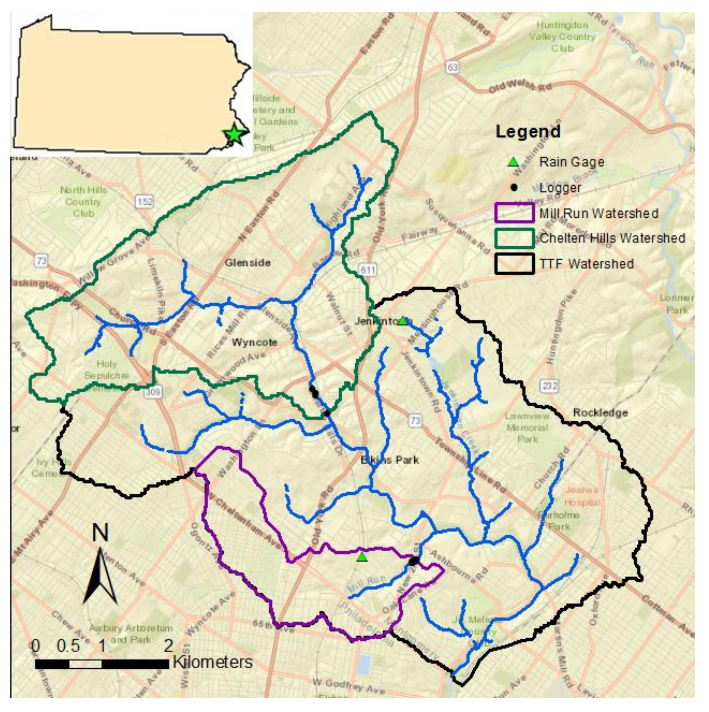
The Tookany/Tacony–Frankford (TTF) Creek flows from Abington Township, Montgomery County and through Philadelphia County before discharging into the Delaware River. Based on calculations done in ArcGIS (Environmental Systems Research Institute, Redlands, CA, USA), the total TTF watershed is 93.6 km2 with 41.6 km2 (44%) of the watershed designated the Tookany Watershed, upstream of the Philadelphia County line. In addition to the main stem, there are five main tributaries in the headwater region. Together, their total length is 34.2 km [32]. The average discharge of the Tookany upon entering Philadelphia County is 0.74 m3/s, based on data obtained from the U.S. Geological Survey stream gauge 01467086. The Tookany watershed mostly overlies mica schist.
Highly urbanized, the watershed is predominately low to medium level development with 51% of the land use classified as low intensity residential composed of single family detached residential housing. Deciduous forest is the second most common land cover at 16% [32]. The 2008 stormwater management plan cites flooding, erosion, sedimentation, groundwater impacts, and pollution as major issues associated with stormwater in the watershed [32].
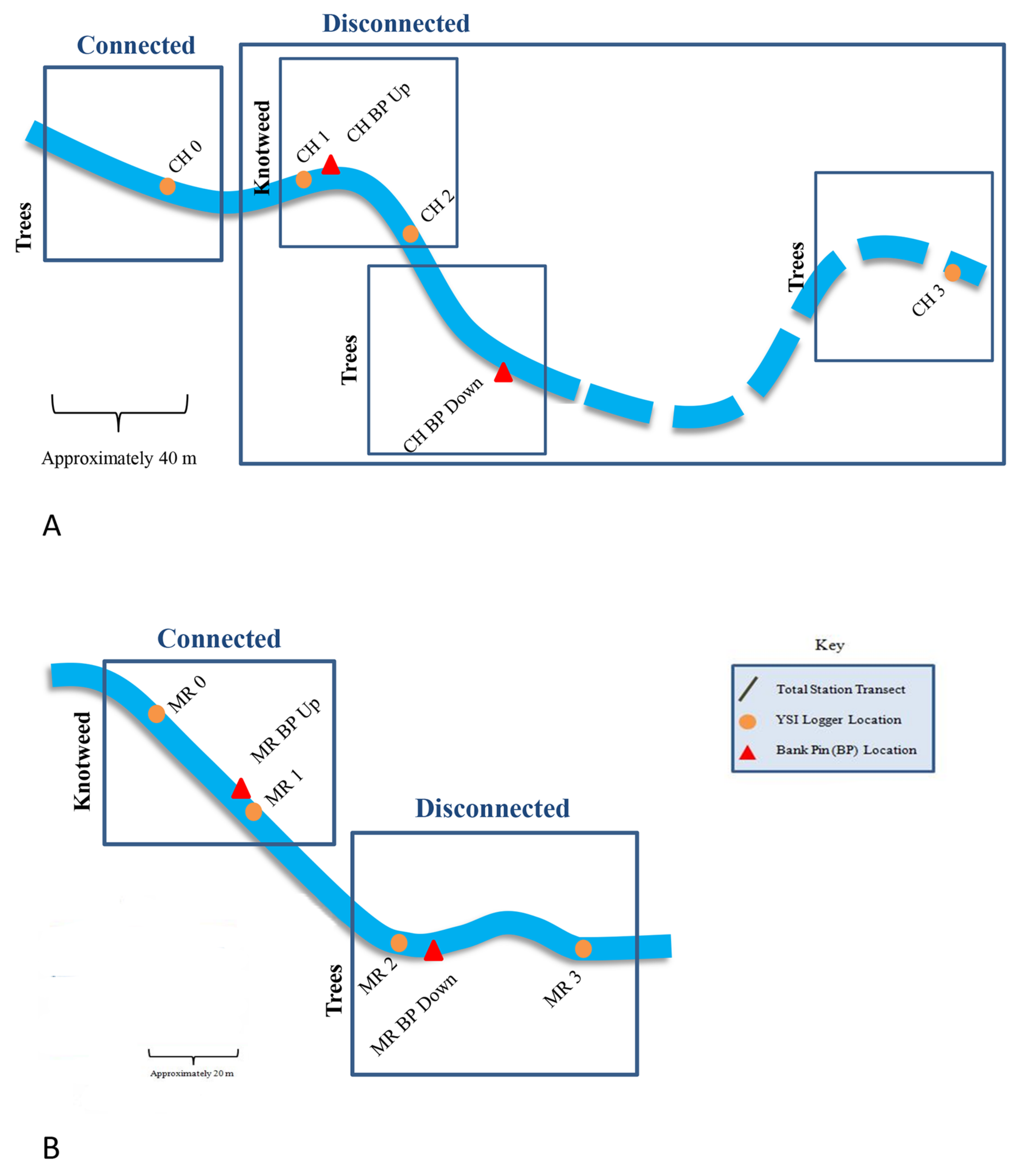
Two reaches were chosen for monitoring within the Tookany Watershed (Figure 1). One reach paralleled Chelten Hills Rd (CH), located on the main stem of the Tookany Creek. The drainage area upstream of the monitoring locations represents 33% of the total Tookany Watershed. Mill Run (MR) is a tributary to the Tookany Creek and monitoring locations represents 93% of the tributary drainage area and 10% of the total Tookany Watershed. Each site had four turbidity loggers (CH 0 through CH 3 and MR 0 through MR 3) and two bank pin monitoring locations (Figure 2) as described in the next section.
Discharge was measured along each reach near loggers 0 and 2. The discharge changed little between logger locations, with the difference being within measurement error. The discharge at Chelten Hills was 0.11 m3/s at baseflow and at Mill Run it was 0.02 m3/s at baseflow.
2.2. Monitoring Erosion
Bank pins and turbidity loggers were used to monitor erosion directly and indirectly, respectively. These methods provide data on temporal and spatial scales within each monitored reach. Four turbidity loggers and two bank pin locations were instrumented in each of the two study reaches.
Bank pins are a method of monitoring erosion or deposition through the installation and measurement of exposed rods. By measuring the amount of pin exposed it is possible to determine the extent of change as well as the rate of change. Bank pins (BP) were installed at two locations with varying riparian characteristics, specifically vegetation and the degree of incision, at each study reach (Figure 2, labeled BP). At Chelten Hills, the bank pins represent erosion rates in a disconnected riparian section dominated by knotweed as well as a disconnected section with trees present. At Mill Run bank pins where installed in a connected reach dominated by knotweed and a disconnected reach dominated by trees. Along the connected reach, a small, less than 0.5 m bank allowed for installation, but the reach was classified as connected due to the interaction between the stream surface and both the floodplain and root structures.
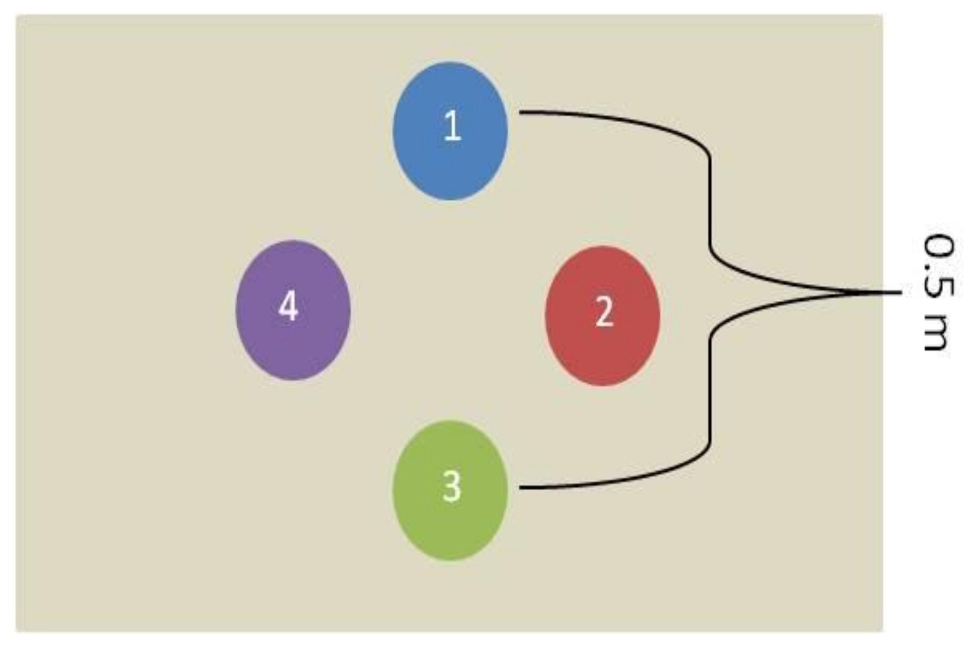
Four erosion pins (0.5 m long garden stakes) were installed perpendicular to the cut bank face. The pins were installed in a diamond pattern (Figure 3). There was approximately 0.5 m between each pin with the bottom pin located just above the waterline present on the date of installation.
The initial length of the exposed pin was recorded and used to establish a starting position of the bank. Subsequent measurements of the exposed pin were used to calculate how much erosion had occurred at each pin location. Bank pins that experienced substantial erosion were reset to 15 cm when in danger of being eroded out of the bank. This occurred twice at the upstream Chelten Hills monitoring point and once at the downstream Mill Run location. The measurement interval ranged from five days to a month. At each site the change in bank position was analyzed individually, then averaged. The average of the four bank pins was used to compare different reaches as the rates were similar within sites [33].
Turbidity loggers (YSI OMS 600, Yellow Spring Instruments, Yellow Springs, OH, USA) were installed at four sites on the main stem near Chelten Hills Road and four sites on Mill Run from May 2015 through March 2016. The loggers were numbered 0 through 3 from upstream to downstream. All loggers were calibrated prior to deployment. The YSI loggers use an optical sensor to record turbidity in nephelometric turbidity unit (NTU). In addition to turbidity loggers, water level loggers (Onset HOBO U20-04, Onset Computer Corporation, Bourne, MA, USA) were installed at each location to relate water level to turbidity.
Loggers were installed near the banks. Equipment installed in meanders were placed on the cut bank side. Loggers CH 0 through CH 3 at Chelten Hills were installed in the middle of a connected native trees riparian zone, as well as the beginning and end of a highly disconnected riparian zone with knotweed. There were 80 m between loggers CH 0 and CH 1 and 30 m between loggers CH 1 and CH 2. The distance between the CH 2 and CH 3 was approximately 300 m. CH 3 was placed for a longitudinal study to examine spatial variability. At Mill Run MR 0 and MR 1 were installed at the beginning and end of the connected reach dominated by knotweed and MR 2 and MR 3 were installed at the beginning and end of a disconnected reach with trees. This downstream reach was separated from the upstream reach by both large woody debris and a stormwater inlet channel. There was approximately 30 m between each logger.
Turbidity measurements were not directly related to total suspended sediment as no sediment calibration curve was created for the logger locations. However, a relationship between total suspended sediment and turbidity is typically linear [6,10,11,13,34,35] and was likely similar among sites given the sediment characteristics.
2.3. Streambed and Bank Characterization
Monitoring locations were chosen based on accessibility, vegetation type, and degree of incision, and the habitats were classified based on these characteristics. Riparian type was determined based on the presence of knotweed versus trees versus a mixture. Banks were classified as incised or disconnected from its floodplain if roots did not interact with the water. Connected reaches showed interaction between the stream surface and both the floodplain and root structures. These reaches could have up to 0.5 m of incision. Highly disconnected reaches showed at least 2 m of incision, which indicates longer term erosion, while reaches termed disconnected had between 0.5 and 1.5 m of incision. The geomorphic position and sediment were characterized at each logger location. The geomorphic position was characterized in terms of pool, riffle, or run and degree of incision.
The streambed was characterized for embeddedness to evaluate the influence of local conditions on turbidity. Embeddedness is defined as the extent that coarse substrates, such as gravel and boulders are surrounded and covered by sand other fine sediments. The embeddedness of the streambed was surveyed by evaluating how easily coarse grains on the surface of the streambed could be dislodged. A 60 × 60 cm grid was constructed with markers placed every 5 cm to ensure that measurement positions were unbiased. The grid was set up near the center of the stream, directly adjacent to each turbidity logger except for CH 3 which was omitted from the sediment characterization study due to its distance from the other sites. A scale of 0 to 5 was used to characterize the ease at which the grains were removed [36]. The scale represented increasing embeddedness with a result of 0 representing a node where a coarse grain was present and could be dislodged with no resistance. A result of 5 indicated that the grain could not be pulled out of the streambed nor could it be moved at all (Table 1). If there were no coarse grains present at the grid node, a notation of “S” was recorded to signify that only sand/loose sediment was present.
Streambed sediment texture was also measured. Samples were collected with a shovel from the top 3–5 cm for sediment characterization on a gravel, sand, silt + clay trilinear plot. Fines are likely to be removed by streamflow when using a shovel to collect samples from the bed, but the proportions of the other sediment sizes are still commonly used to compare bedding characteristics. Sieves ranging from 0.063 mm to 25.4 mm were used to separate samples into gravel, sand, and silt + clay. Clasts larger than 25.4 mm were not included in the plots as their weight would significantly bias the results.
2.4. Data Analysis
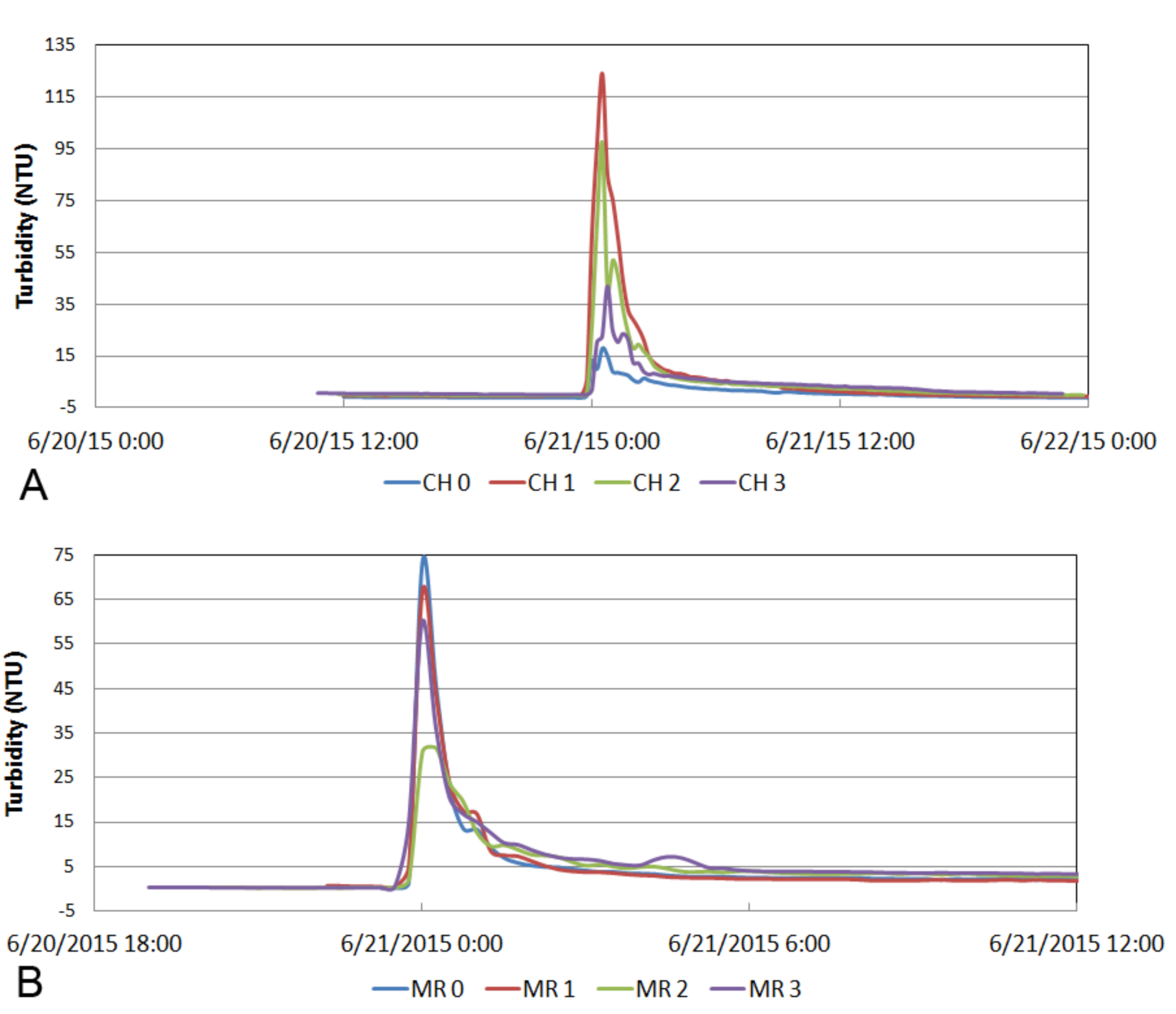
The turbidity response to storms was characterized by the peak value. Turbidity responses generally had a rapid ascending limb followed by a gradual return to equilibrium conditions (Figure 4). The peaks were distinct for each storm. These turbidity peaks were compared to site characteristics across different storm events to determine whether turbidity differed based on vegetation, degree of incision, bed sediment grain size, or storm characteristics. Not all loggers at each site recorded during storms due to battery failure or temporary sediment clogging, but the number of events is noted in the analysis and the same storms were compared at each site.
Storms were characterized by total precipitation and intensity. To be classified as a storm, precipitation needed to last over one hour. If there was a greater than 10-h break in precipitation a new storm event was declared as water level responses tended to recover within that time period as based on visual inspection. Two rain gauges were used to identify precipitation events. Data were downloaded from the Philadelphia Water Department rain gauge PWD_30 closer to Mill Run and from a Villanova University rain gauge near Chelten Hills starting on 28 July 2015 (Figure 1). In addition, the water level logger data provided a measure of storm response. The water level peaks were compared to turbidity peaks using linear regression.
To determine the relationship among turbidity and riparian and streambed characteristics the statistical software package, number crunching statistical software (NCSS, Kaysville, UT, USA), was used. When analyzing two groups the Mann-Whitney U test was used. For example, the comparison of tree and knotweed vegetation types were compared with this method. If greater than two groups were being compared Kruskal-Wallis one-way analysis of variance (ANOVA) was used. Both analyses were chosen as they could rank data that was not normally distributed and can be used on unequal sample sizes. When only two categories were present for comparison t-tests were used, otherwise ANOVA was used. Because several of the parameters used rank statistics rather than continuous variation, multi-variate analysis was not applicable. Filters were applied to separate how vegetation type, degree of incision, antecedent conditions, and seasonality influenced turbidity levels. Antecedent conditions considered rain events within the last five days as wet conditions. If no storms had occurred within five days conditions were considered dry. Seasonality was examined using foliage as an indicator by splitting the dataset in mid-November. The amount and intensity of precipitation were also compared between foliated and non-foliated conditions to ensure that there was no change in storm size that might influence turbidity results. A p = of 0.05 was used as the threshold of determining statistical significance at the 95% confidence interval. Ranks were used for parameters that did not vary continuously such as embeddedness and vegetation, and for parameters with distinct groups such as incision, and grain size distribution. Results are presented as box plots showing the median value, first and third quartiles, and the maximum and minimum values with outliers shown for values beyond 1.5 times the interquartile range.
3. Results
3.1. Logger Site Comparison
The vegetation along the banks included mature hardwood trees with visible root structure on the banks. Sometimes knotweed would be present in reaches with tress, but when the presence of tree roots was observed the section was labeled as tree-covered (Table 2). In other reaches, only knotweed was present. The disconnected banks were 1–1.5 m high, with highly incised reaches showing at least 2 m of bank height. The stream width at Chelten Hills was 2–3 m, except CH 0 where it extended 4.75 m, resulting in a depth to width ratio (D:R) of 0.7 and 0.8 for highly disconnected banks and 0.3 for the connected bank (Table 2). Mill Run was generally wider, 6–7.5 m wide except at MR 3 which narrowed to 4.5 m. The depth to width ratio was 0.2 except at MR 3 where is was 0.4.
The streambed sediments were characterized at each logger site except for CH 3 (Table 2). Sand content in pools ranged from 29.4 to 92.6%, with the highest sand content appearing at Mill Run logger 2 (MR 2). At Mill Run the sediment collected from pools was found to have higher proportions of sand to gravel than those sampled from the run. This pattern does not hold true at Chelten Hills where the pool sample (CH 2) contains 16.0% less sand than the sample taken from the run (CH 0). The amount of gravel in runs ranged from 54.1 (CH 0) to 61.9% (MR 1). The greatest amount of gravel was found within riffles at both sites with CH 2 and MR 0 containing 74.3% and 71.7% gravel, respectively.
In both streams, the embeddedness survey showed the majority of sediment (76 to 100%) was either sand/loose sediment (S) or loose grains (0–2) and only two sites showed more than 20% embedded grains of some degree (Table 2). The two sites with strongly embedded grains were in riffles, and one of the runs has somewhat embedded grains.
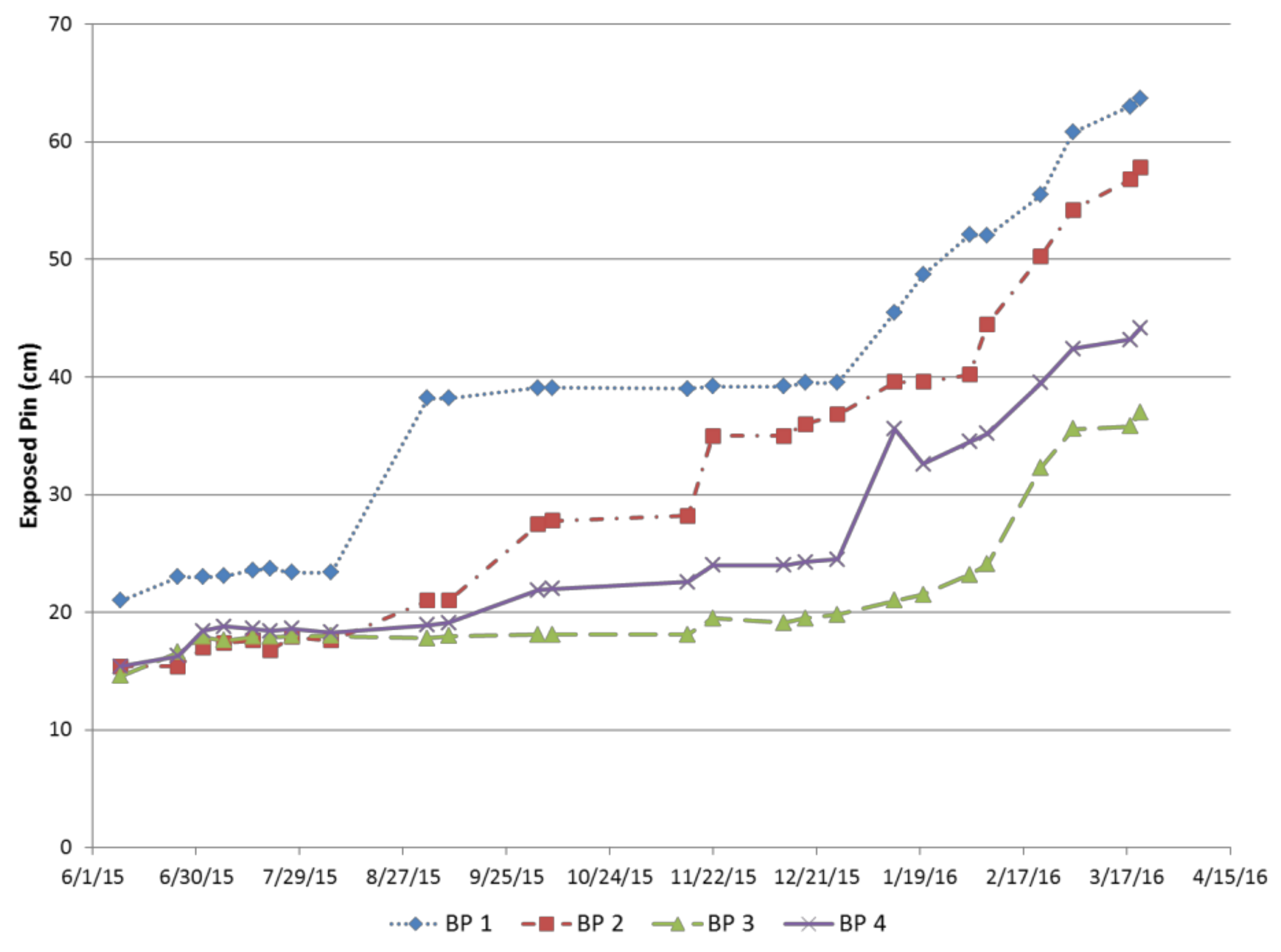
3.2. Bank Pins: Erosional Events
Bank pin measurements showed erosion occurred episodically, but with an overall trend that differed for each site. For example, at CH BP Upstream located on a highly incised cut bank with mixed tree and knotweed vegetation, the degree of erosion varied during erosional events with no one event being recorded in all bank pins (Figure 5). The variation between the four pins illustrates the limitations in using bank pins to estimate erosion rates over larger scales. An extended change in erosion rate occurred over the winter in three of the bank pins locations, including CH BP Upstream. At the CH BP Downstream, little erosion was observed. Because of this change in rate, the average erosion was calculated separately for summer and early fall versus later fall and winter. The degree of erosion at each of these pins was higher than at the other sites; thus, the rates for each site were compared as an average rate.
The trend in average erosion rates for each site was the same across both seasons (Figure 6). The site with disconnected banks and knotweed (CH BP Upstream) had the highest rate followed by knotweed on a connected bank (MR BP Upstream). The lowest rates were observed at the two sites with trees, both with disconnected banks (MR and CH BP Downstream).
3.3. Turbidity Response to Storm Events
Continuous turbidity loggers recorded increases in turbidity for 43 storm events at Chelten Hills and Mill Run. Logger response was compared for logger location, with and without foliage, degree of incision, riparian cover, geomorphic position, and streambed grain size. Results are presented as box plots and evaluated for statistically significant differences.
Linear regression between the water level peaks and the turbidity peaks showed the expected relationship between higher storm flow and higher turbidity with one exception (Table 3). Most of the R2 were 0.6 or better, but at MR 2 the regression was only 0.25. The lower correlation at this site was attributed to woody debris upstream which caught debris; periodic release of debris and associated sediment could have led to a noisier turbidity signal at this site. However, neither the mean nor the standard deviation was higher at MR 2, so the woody debris did not contribute significantly to the sediment loading downstream. Although higher velocity associated with larger storms is expected to increase turbidity, the correlations at these sites suggest that other factors are also important in explaining the turbidity variation.
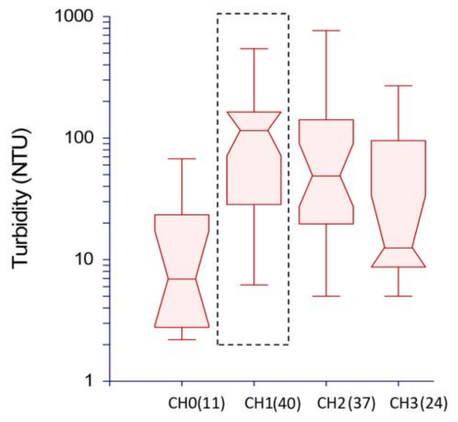
Comparison of box plots showed that the turbidity response increased between loggers CH 0 and CH 1, which represented the transition from the connected with trees to a disconnected reach with knotweed (Figure 7). The change in turbidity between these loggers was found to be statistically significant (p = 0.006) using Kruskal-Wallis One-Way ANOVA with a difference in mean turbidity of 81.7 NTUs. No significant difference (p = 0.665) was found between loggers CH 1 and CH 2 at the 95% confidence interval. CH 3 had a mean turbidity of 46.4 NTU lower than that of CH 2. However, because the turbidity at CH 3 had a high variability, this difference in mean turbidity was not statistically significant (p = 0.127) at the 95% confidence interval.
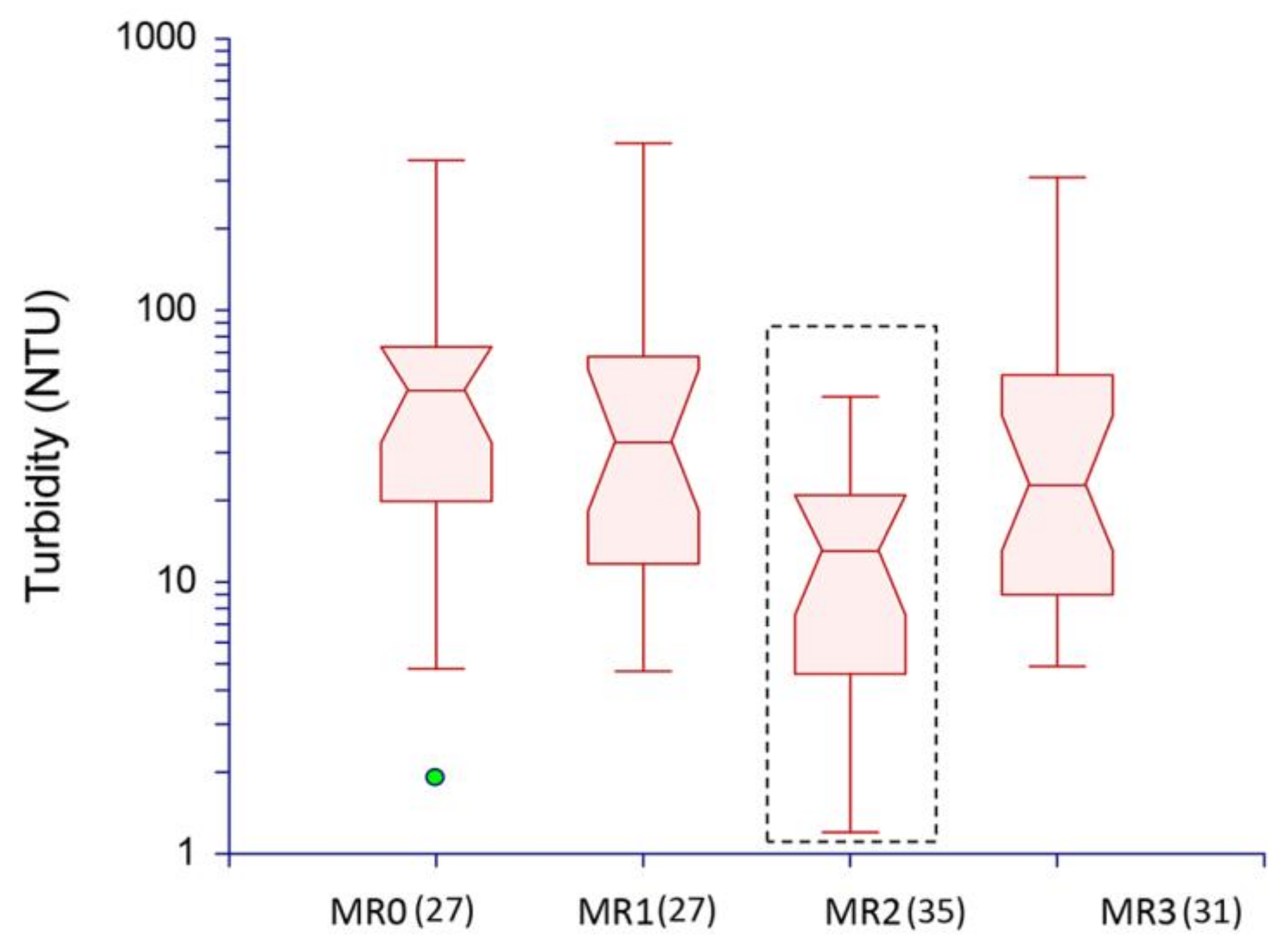
The range of turbidity response at Mill Run was somewhat less than that of Chelten Hills. The mean turbidity reading of logger MR 2 was lower than the other loggers (42.3 NTUs lower than logger MR0, 49.4 NTUs lower than logger MR 1, and 25.0 NTUs lower than logger MR 3). It was also found to be statistically different (p = 0.009) from loggers MR 0 and MR 1, but not from MR 3 (Figure 8). This logger was located at the transition from knotweed to trees, but also located on a disconnected reach. Thus, the logger with statistically lower turbidity at Mill Run was located in a reach with trees and the logger with statistically higher turbidity at Chelten Hills was located in a reach with knotweed.
Neither the geomorphic position nor the grain size clearly distinguished the two logger sites with statistically lower turbidity response, CH 0 and MR 2 (Table 2). CH 0 is located in a run, but CH 3 was also and it was not statistically different than the other Chelten Hills loggers. MR 2 was one of two loggers located in pools. Thus, the two loggers with lower turbidity had different geomorphic position. CH 0 had similar grain size distribution to most of the other loggers (gravely sand). MR 2 was the only logger in sand, but the finer grain size would be expected to lead to higher, not lower turbidity.
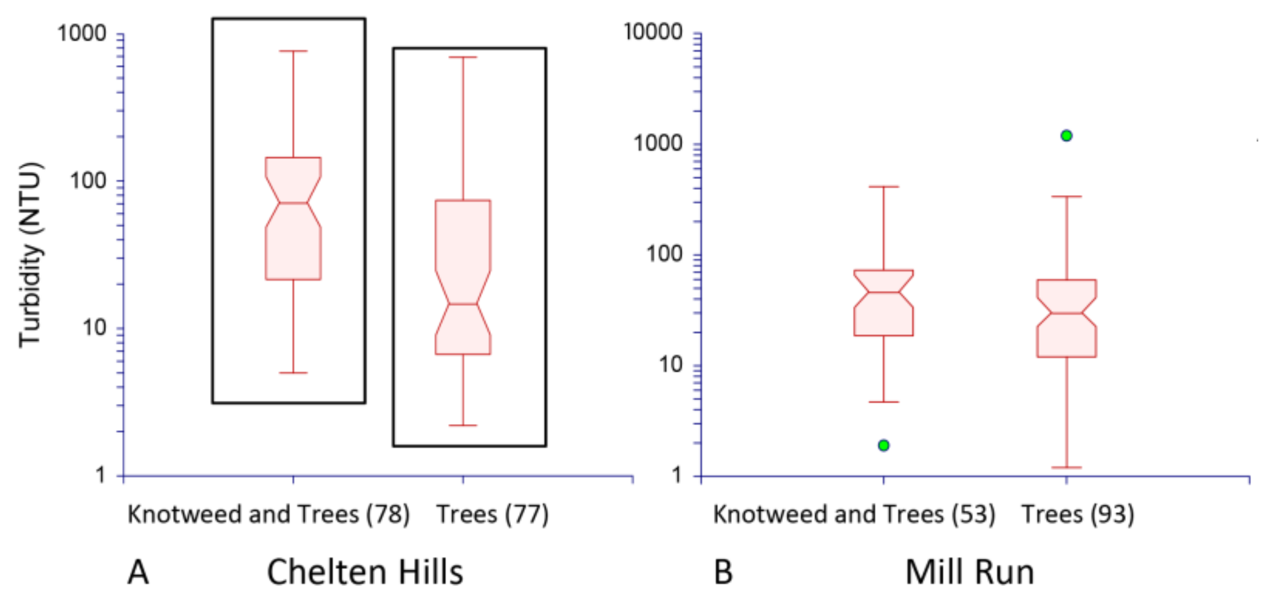
Riparian vegetation was compared at each site by examining the effect of knotweed on turbidity in contrast to sites with mature trees. At Chelten Hills, sites monitored in tree-dominated riparian zones experienced lower turbidity responses than knotweed dominated reaches (Figure 9). Knotweed-dominated reaches had a mean value of 91.3 NTU and tree-dominated reaches had a mean value of 53.3 NTU, a significant difference at the 95% confidence interval (p = 0.02). Mill Run had turbidity responses in knotweed dominated reaches with a mean value of 55.3 NTU and in tree-dominated zones showed a mean value of 54.9 NTU. There was no statistical difference (p = 0.205) between the turbidity responses of different vegetation types at Mill Run. One difference between the sites is that the knotweed section at CH is highly disconnected and it is connected at MR (Figure 2). These results suggested that while the presence of knotweed increases turbidity, the increase is not significant unless the stream is also incised.
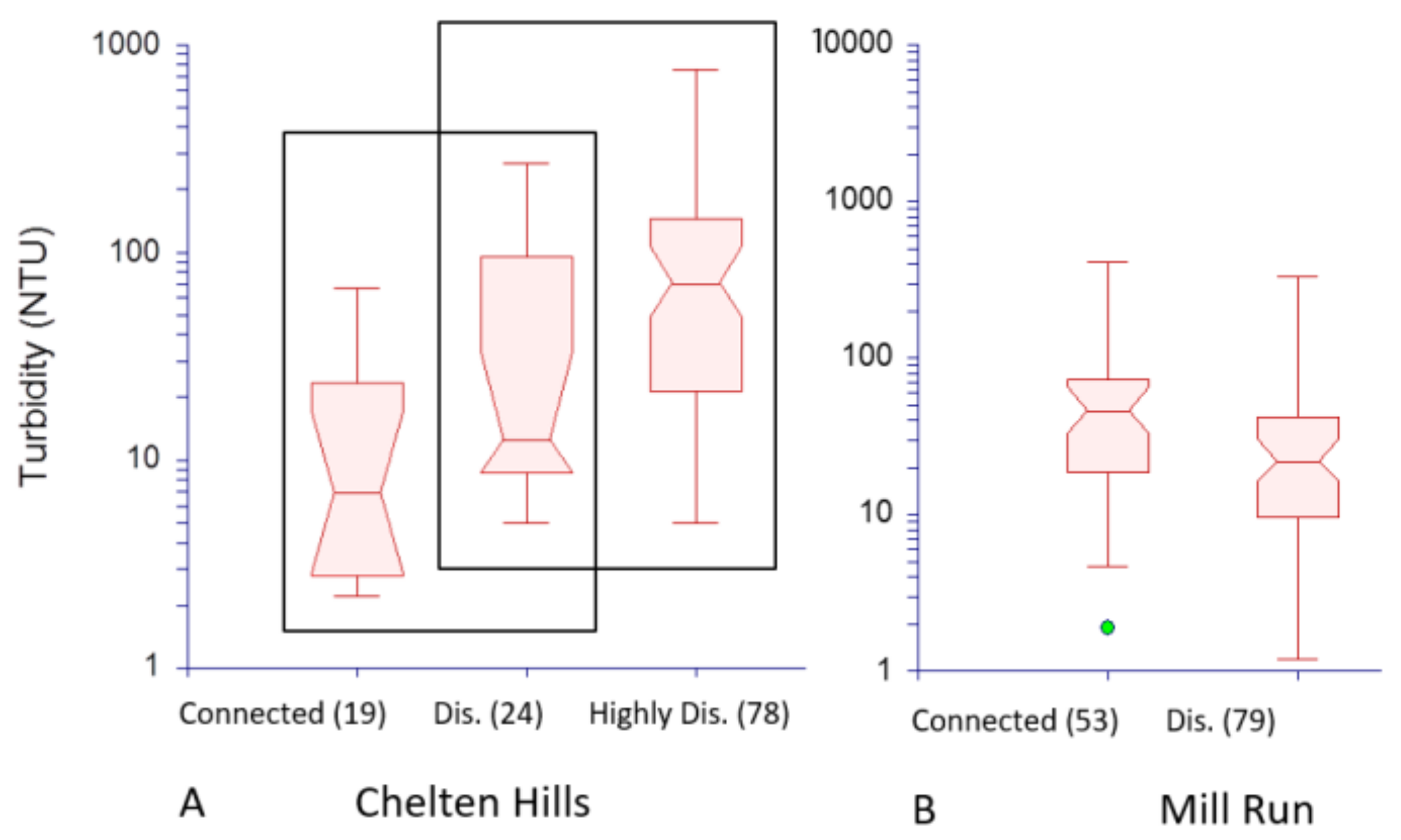
The degree of connectivity was also considered as a factor influencing turbidity response, with the highly disconnected reaches showing greater turbidity. At Chelten Hills, a statistical difference (p = 0.016) was found between the connected and highly disconnected reaches but not between the connected and disconnected reaches or between the disconnected and highly disconnected reaches (Figure 10a). The mean values for connected, disconnected, and highly disconnected were 13.5 NTU, 40.5 NTU, and 86.4 NTU, respectively. When loggers at Mill Run were separated by the degree of incision, the mean response in the connected reach was found to be elevated (55.2 NTU) as compared to the mean response of 32.0 NTU in the disconnected reach, although this difference was not significant (Figure 10b).
The antecedent conditions were also examined to determine if dry conditions yielded different turbidity responses than wet conditions. Dry conditions were defined as a period with no precipitation for five or more days. During wet conditions the difference in turbidity between degrees of incision was statistically significant at both Chelten Hills (p = 0.010) and Mill Run (p = 0.005). There was no statistical difference between varying incision types at Chelten Hills and Mill Run in dry conditions (p = 0.521 and 0.063, respectively).
Two statistical comparisons were made to evaluate the influence of foliage. One test evaluated whether the turbidity response changed at a site when it has foliage versus without foliage. No statistical difference between full and no foliage was found at either at Chelten Hills (p = 0.705) or Mill Run (p = 0.519) at the 95% confidence interval (Figure 11). However, at both sites the mean and standard deviation was found to increase when no foliage was present. Furthermore, the statistical difference between knotweed and trees changed with foliage versus without foliage. At both Chelten Hills and Mill Run there was a significant difference (p = 0.018 and 0.012, respectively) between knotweed and trees when foliage was present. In contrast, there was no difference at either site when foliage was not present (p = 0.335 and 0.106). These differences further emphasize the influence of knotweed on erosion, particularly in the winter months. This increase in turbidity was not associated with corresponding increases in precipitation as neither the amount of precipitation or intensity of precipitation increased during the winter months.
4. Discussion
4.1. Summary of Findings
Erosion was measured directly using bank pins and indirectly using turbidity loggers. Seasonality appeared to influence erosion rates as an increase in erosion can be seen in bank pins after December 2015. This compliments turbidity results which, while not statistically significant, show an increase in the mean turbidity response when no foliage was present.
Riparian characteristics were found to influence erosion rates. For instance, turbidity increased significantly (p = 0.006) from CH 0 to CH 1 upon entering the disconnected reach dominated by knotweed. Statistical analysis (Figure 7) showed vegetation to be the dominant control on turbidity response. However, when comparing the turbidity response between vegetation types at Mill Run, there was not a significant difference. Therefore, while vegetation appears to be the dominant control, the degree of incision impacts whether the increase in erosion associated with prevalent knotweed will result in a significant increase in turbidity. Bank pins also indicated that there were higher rates of erosion in areas with knotweed, although the largest differences were observed for reaches that were also incised.
4.2. Implications for Bank Management
Reconstruction of the entire riparian system is impractical due to the nature of property lines, infrastructure, and cost. By determining which stream characteristics are beneficial and which result in degradation of water quality, measurements on the effects of smaller riparian reaches, such as those conducted for this study, can help promote effective practices [12,15,37]. Without consideration of these local characteristics, management practices have a higher risk of failing.
While many researchers assume the presence of knotweed will lead to higher rates of erosion, previous studies quantifying that assumption are not reflected in the literature. One previous study that provided quantitative analysis focused on rural catchments, which saw an increase in sediment load downstream of knotweed reaches after storm events [27]. However, they could not conclusively evaluate whether this was associated with higher rates of erosion due to limited precipitation events. Other work has used models to predict effects of riparian vegetation [25]. Our research provides quantifiable turbidity responses to storm events in reaches dominated by knotweed within an urban setting. Our study suggests that while the presence of knotweed increases erosion, the corresponding increase in turbidity is only statistically significant in disconnected riparian zones. Therefore, if the goal of riparian restoration is to reduce sediment loads, replacing Japanese knotweed with native vegetation by removing vegetation from the banks is not necessarily effective where incision is minimal. Other management techniques that can be used include, but are not limited to, those that promote in-stream deposition and bank stabilization with rip rap or other engineering structures. Furthermore, if this management technique is used, it is important that cleared riparian zones be maintained. The knotweed at Mill Run was removed as part of a community riparian restoration but was recolonized within ten years. This suggests that the removal of invasives might not be the best long-term solution if there are minimal funds for continued monitoring and maintenance. Maintenance is also needed during the time it takes trees planted for riparian restoration to mature, in order to prevent incision of the bank, loss of trees due to disease, and invasion of exotic species such as Japanese knotweed.
4.3. Implications for Sediment Budgets
In streams where sediment erosion creates impairment, site and catchment scale sediment budgets can be useful. Estimating erosion rates can be difficult, with multiple years of data collection necessary [3,11,15,38]. Once created, sediment budgets can be used to identify areas that should receive direct management.
Sediment erosion calculations in the Tookany Watershed provided evidence for heterogeneity based on specific riparian type in the catchment. Extrapolation to other reaches within the stream could then be used to create a catchment scale budget, based on the influence of specific, small-scale characteristics on erosion. However, this method requires an assumption that the data can be projected to other locations within the catchment. This study had only two bank pin locations per reach. More comparisons of erosion rates between similar reaches would be useful to establish variability before using this type of extrapolation. While the sample size within our study was not large enough to provide a sediment budget, preliminary results indicate that bank pin monitoring and turbidity data can be used to evaluate reach scale variations.
Small-scale studies like those in the Tookany Creek help to show the erosion variability within streams. This is especially true in urban watersheds where increased discharge from impervious surfaces, development adjacent to the stream corridor, and invasive species often culminate in highly impaired waterways. Understanding sediment dynamics to decrease turbidity and sediment levels entering water bodies is needed for improvement of stream health and water quality and monitoring of streams is necessary to design and implement appropriate management practices.
Acknowledgments
This work was supported by a grant from the William Penn Foundation under the Delaware River Watershed Initiative. Field assistance was provided by Chris Witzigman. We are grateful to an anonymous reviewer who helped clarify the text and figures.
Author Contributions
This research was conducted as part of a master’s thesis by Emily Arnold under the direction of Laura Toran. Both authors designed and set up the field study. Emily Arnold collected the data and processed it, and both authors were involved in interpretation.
Conflicts of Interest
The authors declare no conflict of interest.
References
- Walsh, C.J.; Roy, A.H.; Feminella, J.W.; Cottingham, P.D.; Groddman, P.M.; Morgan, R.P.I. The Urban Stream Syndrome: Current Knowledge and the Search for a Cure. J. N. Am. Benthol. Soc. 2005, 24, 706–723. [Google Scholar] [CrossRef]
- Walter, R.; Merritts, D. Natural streams and the legacy of water-powered milling. Science 2008, 319, 299–304. [Google Scholar] [CrossRef] [PubMed]
- Taylor, K.G.; Owens, P.N. Sediments in urban river basins: A review of sediment-contaminant dynamics in an environmental system conditioned by human activities. J. Soils Sediments 2009, 9, 281–303. [Google Scholar] [CrossRef]
- Pizzuto, J.; Schenk, E.R.; Hupp, C.R.; Gellis, A.; Noe, G.; Williamson, E.; Karwan, D.L.; O’Neal, M.; Marquard, J.; Aalto, R.; et al. Characteristic length scales and time-averaged transport velocities of suspended sediment in the mid-Atlantic Region, USA. Water Resour. Res. 2014, 50, 790–805. [Google Scholar] [CrossRef]
- Nelson, E.J.; Booth, D.B. Sediment sources in an urbanizing, mixed land-use watershed. J. Hydrol. 2002, 264, 51–68. [Google Scholar] [CrossRef]
- Davies-Colley, R.J.; Smith, D.J. Turbidity, suspended sediment, and water clarity: A review. J. Am. Water Resour. Assoc. 2001, 37, 1084–1101. [Google Scholar] [CrossRef]
- Underwood, J.; Renshaw, C.E.; Magilligan, F.; Dade, W.B.; Landis, J.W. Joint isotopic mass balance: A novel approach to quantifying channel bed to channel margins sediment transfer during storm events. Earth Surf. Process. Landf. 2015, 40, 1563–1573. [Google Scholar] [CrossRef]
- Hupp, C.; Noe, G.; Schenk, E.R.; Benthem, A.J. Recent and historic sediment dynamics along Difficult Run, a suburban Virginia Piedmont stream. Geomorphology 2013, 180–181, 156–169. [Google Scholar] [CrossRef]
- Schenk, E.R.; Hupp, C.; Gellis, A.; Noe, G. Developing a new stream metric for comparing stream function using a bank–floodplain sediment budget: A case study of three Piedmont streams. Earth Surf. Process. Landf. 2013, 38, 441–784. [Google Scholar] [CrossRef]
- Gao, P. Understanding watershed suspended sediment transport. Prog. Phys. Geogr. 2008, 32, 243–263. [Google Scholar] [CrossRef]
- Wass, P.D.; Leeks, G.J.L. Suspended sediment fluxes in the Humber Catchment, UK. Hydrol. Process. 1999, 13, 935–953. [Google Scholar] [CrossRef]
- Schwartz, J.S.; Dahle, M.; Robinson, R.B. Concentration-frequency-duration curves for stream turbidity: Possibilities for use assessing biological impairment. J. Am. Water Resour. Assoc. 2008, 44, 879–886. [Google Scholar] [CrossRef]
- Skarbøvik, E.; Roseth, R. Use of sensor data for turbidity, pH and conductivity as an alternative to conventional water quality monitoring in four Norwegian case studies. Acta Agric. Scand. Sect. B Soil Plant Sci. 2015, 65, 63–73. [Google Scholar] [CrossRef]
- Minella, J.P.G.; Merten, G.H.; Reichert, J.M.; Clarke, R.T. Estimating suspended sediment concentrations from turbidity measurements and the calibration problem. Hydrol. Process. 2008, 22, 1819–1830. [Google Scholar] [CrossRef]
- Schilling, K.E.; Isenhart, T.M.; Palmer, J.A.; Wolter, C.F.; Spooner, J. Impacts of land-cover change on suspended sediment transport in two agricultural watersheds. J. Am. Water Resour. Assoc. 2011, 47, 672–686. [Google Scholar] [CrossRef]
- Richardson, D.M.; Holmes, P.M.; Esler, K.J.; Galatowitsch, S.M.; Stromberg, J.C.; Kirkman, S.P.; Pysek, P.; Hobbs, R.J. Riparian vegetation: Degradation, alien plant invasions, and restoration prospects. Divers. Distrib. 2007, 13, 126–139. [Google Scholar] [CrossRef]
- Vidon, P.; Allan, C.; Burns, D.; Duval, T.P.; Gurwick, N.; Inamdar, S.; Lowrance, R.; Okay, J.; Scott, D.; Sebestyen, S. Hot Spots and Hot Moments in Riparian Zones: Potential for Improved Water Quality Management. J. Am. Water Resour. Assoc. 2010, 46, 278–298. [Google Scholar] [CrossRef]
- Warren, R.J.; Potts, D.L.; Frothingham, K.M. Stream structural limitations on invasive communities in urban riparian areas. Invasive Plant Sci. Manag. 2015, 8, 353–362. [Google Scholar] [CrossRef]
- Merchant, C. American Environmental History: An Introduction; Columbia University Press: New York, NY, USA, 2007. [Google Scholar]
- Simon, A.; Collison, A.J.C. Quantifying the mechanical and hydrologic effects of riparian vegetation on streambank stability. Earth Surf. Process. Landf. 2002, 37, 527–546. [Google Scholar] [CrossRef]
- Gurnell, A.M. Plants as river system engineers. Earth Surf. Process. Landf. 2014, 39, 4–25. [Google Scholar] [CrossRef]
- Smith, D.G. Effect of vegetation on lateral migration of anastomosed channels of a glacier meltwater river. Geol. Soc. Am. Bull. 1976, 87, 857–860. [Google Scholar] [CrossRef]
- Allmendinger, N.E.; Pizzuto, J.E.; Potter, N.J.; Johnson, T.E.; Hession, W.C. The influence of riparian vegetation on stream width, Eastern Pennsylvania, USA. Geol. Soc. Am. Bull. 2005, 117, 229–243. [Google Scholar] [CrossRef]
- Van Oorschot, M.; Kleinhans, M.; Geerling, G.; Middelkoop, H. Distinct patterns of interaction between vegetation and morphodynamics. Earth Surf. Process. Landf. 2016, 41. [Google Scholar] [CrossRef]
- Konsoer, K.M.; Rhoads, B.L.; Langendoen, E.J.; Best, J.L.; Ursic, M.E.; Abad, J.D.; Garcia, M.H. Spatial variability in bank resistance to erosion on a large meandering, mixed bedrock-alluvial river. Geomorphology 2016, 252, 80–87. [Google Scholar] [CrossRef]
- Tickner, D.P.; Angold, P.G.; Gurnell, A.M.; Mountford, J.O. Riparian plant invasions: Hydrogeomorphical control and ecological impacts. Prog. Phys. Geogr. 2001, 25, 22–52. [Google Scholar] [CrossRef]
- Mummigatti, K. The Effects of Japanese Knotweed (Reynoutria japonica) on Riparian Lands in Otsego County, New York; Report of the Biological Field Station; State University of New York, College of Oneonta: Cooperstown, New York, NY, USA, 2001; pp. 111–119. [Google Scholar]
- Pysek, P.; Prach, K. Plant invasions and the role of riparian habitats: A comparison of four species alien to central Europe. J. Biogeogr. 1993, 20, 413–420. [Google Scholar] [CrossRef]
- Lecerf, A.; Patfield, D.; Boiche, A.; Riipinen, M.P.; Chauvet, E.; Dobson, M. Stream ecosystems respond to riparian invasion by Japanese Knotweed (Fallopia japonica). Can. J. Fish. Aquat. Sci. 2007, 64, 1273–1283. [Google Scholar] [CrossRef] [Green Version]
- Beerling, D.J. The effect of Riparian land use on the occurrence and abundance of Japanese knotweed Reynoutria japonica on selected rivers in South Wales. Biol. Conserv. 1991, 55, 329–337. [Google Scholar] [CrossRef]
- Maskell, L.C.; Bullock, J.M.; Smart, S.M.; Thompson, K.; Hulme, P.E. The distribution and habitat associations of non-native plant species in urban riparian habitats. J. Veg. Sci. 2006, 17, 499–508. [Google Scholar] [CrossRef]
- Borton-Lawson Engineering Inc. Tookany/Tacony-Frankford Watershed Act 167: Stormwater Management Plan, Volume 1—Executive Summary; Philadelphia Water Department: Philadelphia, PA, USA, 2008; pp. 1–250. [Google Scholar]
- Arnold, E.G. Evaluation of Urban Riparian Buffers on Stream Health in the Tookany Watershed, PA. Master’s Thesis, Temple University, Philadelphia, PA, USA, 2016. Available online: http://digital.library.temple.edu/cdm/ref/collection/p245801coll10/id/405730) (accessed on 13 April 2018).
- Rügner, H.; Schwientek, M.; Beckingham, B.; Kuch, B.; Grathwohl, P. Turbidity as a proxy for total suspended solids (TSS) and particle facilitated pollutant transport in catchments. Environ. Earth Sci. 2013, 69, 373–380. [Google Scholar] [CrossRef]
- Gippel, C.J. Potential of turbidity monitoring for measuring the transport of suspended solids in streams. Hydrol. Process. 1995, 9, 83–97. [Google Scholar] [CrossRef]
- Bunte, K.; Abt, S.R. Sample Surface and Subsurface Particle-Size Distributions in Wadable Gravel- and Cobble-Bed Streams for Analyses in Sediment Transport, Hydraulics, and Streambed Monitoring; General Technical Report. RMRS-GTR-74; Department of Agriculture, Forest Service, Rocky Mountain Research Station: Fort Collins, CO, USA, 2001; p. 428. [Google Scholar]
- Polyakov, V.; Fares, A.; Ryder, M. Precision riparian buffers for the control of nonpoint source pollutant loading into surface water: A review. Environ. Rev. 2005, 13, 129–144. [Google Scholar] [CrossRef]
- Lawler, D.M.; Petts, G.E.; Foster, I.D.L.; Harper, S. Turbidity dynamics during spring storm events in an urban headwater river system: The upper Tame, West Midlands, UK. Sci. Total Environ. 2006, 360, 109–126. [Google Scholar] [CrossRef] [PubMed]
Figure 1.
Tookany Watershed and PA state map inset: The Tookany Watershed (black) is 41.6 km2 and is primarily classified as low intensity residential development. Two sub watersheds, Chelten Hills (green) and Mill Run (purple) were monitored using turbidity loggers. There were eight logger locations in the watershed.

Figure 2.
Sketch map of study reaches at Chelten Hills (A) and Mill Run (B) showing the locations and descriptions of each reach. Solid lines are drawn approximately to scale, dashed line indicate change in mapped distance. Stream flow is from station 0 to 3. Bank incision and riparian cover defined by boxed areas.

Figure 3.
Bank pin installation diagram. Four bank pins were installed horizontally into the stream bank in a diamond pattern at each site. The length of the exposed pin was used to calculate erosion.
Figure 3.
Bank pin installation diagram. Four bank pins were installed horizontally into the stream bank in a diamond pattern at each site. The length of the exposed pin was used to calculate erosion.

Figure 4.
Example turbidity response to storm event. Turbidity response to storm on 21 June 2015 at Chelten Hills (A) and Mill Run (B).
Figure 4.
Example turbidity response to storm event. Turbidity response to storm on 21 June 2015 at Chelten Hills (A) and Mill Run (B).

Figure 5.
Chelten Hills upstream bank pin results. The change in the exposed bank pin as a measure of erosion. Increases in the rate of erosion are designated as erosional events.
Figure 5.
Chelten Hills upstream bank pin results. The change in the exposed bank pin as a measure of erosion. Increases in the rate of erosion are designated as erosional events.

Figure 6.
Total erosion at bank pin locations. The total erosion at each location from July to October 2015 (A) and October 2015 to March 2016 (B). The greatest amount of erosion occurred at the upstream highly disconnected reach containing mixed knotweed (CH BP Up) followed by a connected reach with knotweed (MR BP up). The least amount of erosion occurred at the downstream disconnected reach containing trees (CH BP Down) followed by a disconnected reach with trees (MR BP Down).

Figure 7.
Turbidity response at Chelten Hills by logger. The turbidity response for each logger was plotted and analyzed with ANOVA. Logger CH 0 was found to have a statistically lower turbidity response than loggers CH 1 and CH 2 but no statistical difference from other loggers. Numbers in parentheses indicate the number of storms included in the analysis.

Figure 8.
Turbidity response at Mill Run by logger. The turbidity response for each logger was plotted and analyzed with ANOVA. Logger MR 2 was found to have a statistically different from loggers MR 1 and MR 2. Numbers in parentheses indicate the number of storms included in the analysis.
Figure 8.
Turbidity response at Mill Run by logger. The turbidity response for each logger was plotted and analyzed with ANOVA. Logger MR 2 was found to have a statistically different from loggers MR 1 and MR 2. Numbers in parentheses indicate the number of storms included in the analysis.

Figure 9.
Turbidity response by vegetation. Outlined box plots indicate a statistical difference. When loggers were separated by vegetation type there was a statistical difference between mixed vegetation and trees only at Chelten Hills (A) but no statistical difference between the vegetation types at Mill Run (B). The logger site with trees at Chelten Hills was also highly incised.

Figure 10.
Turbidity response by degree of incision. Outlined box plots indicate a statistical difference. When loggers were separated by degree of incision there was a statistical difference between connected and highly disconnected reaches at Chelten Hills (A) and there was no statistical difference between the connected and disconnected reaches at Mill Run (B).

Figure 11.
Turbidity Response to Change in Foliage: Turbidity data at loggers were analyzed to determine the influence of seasonality, based on the presence of foliage, at Chelten Hills (A) and Mill Run (B). While the mean turbidity does increase at both sites when no foliage was present, this change was not found to be significant at either site.


Table 1.
Embeddedness scale.
| Scale | Description |
|---|---|
| S | Sand, loose sediment |
| 0 | Completely loose |
| 1 | Dislodges easily |
| 2 | Dislodges with little resistance |
| 3 | Dislodges with some difficulty |
| 4 | Can move around but cannot dislodge |
| 5 | Not removable, no movement |
Table 2.
Site characteristics for turbidity logger locations. Loggers in bold showed statistically different response from some of its neighbors.
Table 2.
Site characteristics for turbidity logger locations. Loggers in bold showed statistically different response from some of its neighbors.
| Logger | Connectivity | D:R | Vegetation | Grain Size | Geomorph | Embeddedness |
|---|---|---|---|---|---|---|
| CH 0 | Connected | 0.3 | Trees | Gravel | Run | Loose 79% |
| CH 1 | Highly Disconn | 0.8 | Knotweed | Gravel | Riffle | Loose 92% |
| CH 2 | Highly Disconn | 0.7 | Knotweed | Gravel | Pool | Loose 100% |
| CH 3 | Disconnected | Trees | Run | |||
| MR 0 | Connected | 0.2 | Knotweed | Gravel | Riffle | Loose 76% |
| MR 1 | Connected | 0.2 | Knotweed | Gravel | Run | Loose 98% |
| MR 2 | Disconnected | 0.2 | Trees | Sand | Pool | Loose 100% |
| MR 3 | Disconnected | 0.4 | Trees | Sandy gravel | Pool | Loose 99% |
Table 3.
Linear regression between water level peak and turbidity peak.
| Logger | R2 |
|---|---|
| CH 0 | 0.60 |
| CH 1 | 0.84 |
| CH 2 | 0.77 |
| CH 3 | 0.59 |
| MR 0 | 0.73 |
| MR 1 | 0.76 |
| MR 2 | 0.25 |
| MR 3 | 0.75 |
© 2018 by the authors. Licensee MDPI, Basel, Switzerland. This article is an open access article distributed under the terms and conditions of the Creative Commons Attribution (CC BY) license (http://creativecommons.org/licenses/by/4.0/).
Share and Cite
MDPI and ACS Style
Arnold, E.; Toran, L. Effects of Bank Vegetation and Incision on Erosion Rates in an Urban Stream. Water 2018, 10, 482. https://doi.org/10.3390/w10040482
AMA Style
Arnold E, Toran L. Effects of Bank Vegetation and Incision on Erosion Rates in an Urban Stream. Water. 2018; 10(4):482. https://doi.org/10.3390/w10040482
Chicago/Turabian StyleArnold, Emily, and Laura Toran. 2018. "Effects of Bank Vegetation and Incision on Erosion Rates in an Urban Stream" Water 10, no. 4: 482. https://doi.org/10.3390/w10040482
Note that from the first issue of 2016, this journal uses article numbers instead of page numbers. See further details here.