Predictive Uncertainty Estimation in Water Demand Forecasting Using the Model Conditional Processor

Abstract

In a previous paper, a number of potential models for short-term water demand (STWD) prediction have been analysed to find the ones with the best fit. The results obtained in Anele et al. (2017) showed that hybrid models may be considered as the accurate and appropriate forecasting models for STWD prediction. However, such best single valued forecast does not guarantee reliable and robust decisions, which can be properly obtained via model uncertainty processors (MUPs). MUPs provide an estimate of the full predictive densities and not only the single valued expected prediction. Amongst other MUPs, the purpose of this paper is to use the multi-variate version of the model conditional processor (MCP), proposed by Todini (2008), to demonstrate how the estimation of the predictive probability conditional to a number of relatively good predictive models may improve our knowledge, thus reducing the predictive uncertainty (PU) when forecasting into the unknown future. Through the MCP approach, the probability distribution of the future water demand can be assessed depending on the forecast provided by one or more deterministic forecasting models. Based on an average weekly data of 168 h, the probability density of the future demand is built conditional on three models’ predictions, namely the autoregressive-moving average (ARMA), feed-forward back propagation neural network (FFBP-NN) and hybrid model (i.e., combined forecast from ARMA and FFBP-NN). The results obtained show that MCP may be effectively used for real-time STWD prediction since it brings out the PU connected to its forecast, and such information could help water utilities estimate the risk connected to a decision.

1. Introduction

The variation of the water consumption pattern during the day and week is due to several factors, namely climatic and geographic conditions, commercial and social conditions of people, population growth, technical innovation, cost of supply and condition of water distribution system (WDS) [1,2]. Hence, an accurate short-term water demand (STWD) forecast is required for continuous supply of water to consumers with appropriate quality, quantity and pressures [2]. Several predictive models have been proposed to solve water utility operational decision problems [2,3,4,5,6,7,8,9,10,11]. It has been reported in the scientific literature that predicting with hybrid models gives the best forecast for STWD prediction [2,12,13,14,15]. However, hybrid forecast is deficient for the kind of operational planning decisions that water utilities make when future demand is uncertain [7]. This is because it does not take into account the real uncertainty connected to the future level of demand, and this is a serious limitation [2,7,16,17,18]. Moreover, given that the actual objective of WDS management is not improving demand forecasts per se, but rather to more reliably guarantee short term user’s demand, the problem must be formulated in terms of decision under uncertainty [16,17]. The Bayesian Decision approach is one of the best ways to solve this problem [19,20]. With it, utility function is most often a subjective cost function expressing the propensity of the decision maker to risk and its expected value. Therefore, forecasting the entire predictive density instead of the sole expected value is required, and this can guarantee more reliable and robust decisions [16].

Several authors [16,17,18,21,22,23,24,25] confirmed that it is absolutely necessary to take into account predictive uncertainty (PU), most especially when the predictive models considered are applied within the framework of water management procedures or to support decision-making [21]. According to [16,18], PU is described by the probability distribution of the future (real) value of the predict, which is conditional on the knowledge available at the time of forecasting. To understand and analyse the overall level of the PU connected to STWD forecast, model uncertainty processors (MUPs) are considered [16,26,27]. Amongst other MUPs (e.g., the Bayesian Model Averaging (BMA) [26], Hydrological Uncertainty Processor (HUP) [27]), the Model Conditional Processor (MCP) proposed by [16] is used in this paper. MCP is an uncertainty post-processor that allows the combination of one or more forecasting models to produce a predictive density instead of a single valued forecast [16,17]. The motivation for the selection of MCP is based on the recent applications that have proven its validity and robustness [16,17,18].

Furthermore, decisions such as releasing sufficient amount of water to users may be linked to losses such as loss in users credibility, or more consistently in terms of contractual penalties if the objective is not met [16,24]. At the same time, releasing too much water may lead to wastes, thus to potential economical losses. This is why, by means of a predictive density of future demand, one should compromise between the cost of water, including loss of future opportunities injected into the water distribution network (WDN) to meet future demand and the expected value of losses if the demand objectives are not met. The point is that once the decision is made on how much to inject into the WDN, what is injected is a real physical quantity which has a real cost also in terms of lost opportunities, while the economical losses depending on the future actual demand are still uncertain. This is why, to compromise between the real costs for wasting water and the expected losses for not meeting demand, one needs first of all to assess the probability of future demand, conditional on all our available knowledge, and use this information to estimate the future expected losses by integrating the loss function, which depends on demand, times the probability of demand, over the entire domain of possible demands [18,24,28]. Models are the tools to allow us to correctly assess such an uncertainty, but they are not the final goal. Many researchers in the field of hydrology have looked into the problem of assessing the PU connected to a real-time flood forecasting system using the MCP [16,17]. However, to our knowledge, only Alvisi et al. [18] have used MCP to assess the PU within the framework of water demand forecasting on the basis of the forecasts generated by using two deterministic models, namely a cyclicity and persistence based model (Patt-for) and a feed-forward back propagation neural network (FFBP-NN).

Based on the above information, the main contribution of this paper is to apply the MCP approach to demonstrate how a number of comparatively good (or well performing) deterministic models, namely autoregressive-moving average (ARMA), FFBP-NN and hybrid model (combined forecast from ARMA and FFBP-NN) may improve our knowledge, thus estimating the predictive uncertainty when forecasting into the unknown future. This motivation is based on the fact that these models (e.g., hybrid model) are better deterministic models in the current state of the art [2], and have not been tested in assessing the predictive density in another paper before in this perspective. To achieve this aim, the probability density of the future demand is developed based on the forecasts generated by ARMA, FFBP-NN and the hybrid model. Based on an average weekly data of 168 h, the forecasting performances of ARMA, FFBP-NN, hybrid model and MCP are assessed. Furthermore, MCP is used to estimate the PU connected to the STWD forecast. Finally, in this work, we demonstrate how to verify the correctness of the estimated predictive probability by comparing the predicted conditional density to the sampling density of prediction errors via a graphical/statistical acceptance-rejection test. This is an essential step not present in previous works (for instance in [18]) to guarantee that the assessed probability density can be reliably used to estimate the expected losses in decision-making.

2. Model Conditional Processor (MCP)

MCP is a Bayesian method (i.e., uncertainty post-processor) used to estimate the PU, which is conditional on a set of historical observations and the corresponding values predicted by one or more deterministic forecasting models [16,17,18,28,29]. In this paper, we demonstrate how to use the models’ information to improve our knowledge on the future demand, in terms of variance of prediction errors, by building the probability density of the future demand conditional on the predictions generated by ARMA, FFBP-NN and hybrid model through the MCP approach.

Todini [16] developed the MCP approach with the aim of estimating the predictive distribution of a given predictand conditional upon one or more model forecasts, on the basis of the following useful properties of the multi-Normal distribution [30]: If a real valued random vector x $ϵ$ ${\Re }^{j+k}$, $j\ge 1,k\ge 1$, normally distributed $x\approx N({\mu }_x,{\mathsf{\Sigma }}_{xx})$ with mean ${\mu }_x$, and variance-covariance matrix ${\mathsf{\Sigma }}_{xx}$, is partitioned into two vectors $x=\left[\begin{array}{c}y\\ \widehat{y}\end{array}\right]$, where $yϵ{\Re }^j$ and $\widehat{y}ϵ{\Re }^k$, then the mean, ${\mu }_x=\left[\begin{array}{c}{\mu }_y\\ {\mu }_{\widehat{y}}\end{array}\right]$ and the variance matrix, ${\mathsf{\Sigma }}_{xx}=\left[\begin{array}{cc}{\mathsf{\Sigma }}_{yy}& {\mathsf{\Sigma }}_{y\widehat{y}}\\ {\mathsf{\Sigma }}_{\widehat{y}y}& {\mathsf{\Sigma }}_{\widehat{y}\widehat{y}}\end{array}\right]$, and the two partitions y and $\widehat{y}$, will be normally distributed, i.e., $y\approx N({\mu }_y,{\mathsf{\Sigma }}_{yy})$ and $\widehat{y}\approx N({\mu }_{\widehat{y}},{\mathsf{\Sigma }}_{\widehat{y}\widehat{y}})$.

Under this assumption, one can derive the distribution of each partition conditional on the other one. Therefore, the distribution of y conditional on $\widehat{y}$, is the normal distribution $N({\mu }_{y|\widehat{y}},{\mathsf{\Sigma }}_{yy|\widehat{y}})$ with mean

$${\mu }_{y|\widehat{y}}={\mu }_y+{\mathsf{\Sigma }}_{y\widehat{y}}{\mathsf{\Sigma }}_{\widehat{y}\widehat{y}}^{-1}(\widehat{y}-{\mu }_{\widehat{y}})$$

(1)

and variance co-variance matrix

$${\mathsf{\Sigma }}_{yy|\widehat{y}}={\mathsf{\Sigma }}_{yy}-{\mathsf{\Sigma }}_{y\widehat{y}}{\mathsf{\Sigma }}_{\widehat{y}\widehat{y}}^{-1}{\mathsf{\Sigma }}_{\widehat{y}y}$$

(2)

According to [16,18], the MCP method involves the conversion of historical observations and the corresponding predicted values into a normal space using the Normal Quantile Transform (NQT) in order to arrive analytically at an estimate of the joint distribution of the real and forecasted values and hence at a conditional distribution of the real values given the forecasted ones. However, in this paper, we are in the most favourable case since the conversion into and return from the Gaussian space and the problem of the tails fitting are not necessary. Thus in this paper, the observations and model forecasts generated by ARMA, FFBP-NN and the hybrid model are essentially Gaussian.

The MCP approach was here implemented to assess the predictive density of the demand conditional to the hybrid predictions based on the ARMA, FFBP-NN and hybrid model, the latter taken as the third model. The importance of including the hybrid model lays in the fact that in the multi-variate approach described by Equations (1) and (2), the weights and the resulting variance depend directly on ${\mathsf{\Sigma }}_{y\widehat{y}}$ the covariance matrix between observations and model forecasts and inversely on ${\mathsf{\Sigma }}_{\widehat{y}\widehat{y}}$ the covariance matrix among the model forecasts. In layman’s terms, as a model contributes to the information, the correlation is higher between its forecast and the observations and the forecasts are less correlated with the other model forecasts. As it stands, the hybrid model, a linear combination between the ARMA and FFBP-NN models, has a high correlation with the observations and to a lesser extent with the single ARMA and FFBP-NN models, which allows for the provision of a small amount of important additional information.

3. Case Study Description and Discussion of Results

The predictive performances of ARMA, FFBP-NN, the hybrid model and the MCP are assessed based on a 168 h (one week) long set of data sampled at hourly time steps estimated from observations by averaging eight weeks of observations (see Figure 1). These averages were the only available data from a case study site located in a hydraulic zone in the small city of Alquerias (Murcia) in south-eastern Spain, which has a population of approximately 5000 consumers and an extension of nearly 8 ${\mathrm{km}}^2$ [31]. The number of data used for the calibration and validation sets are approximately 60% and 40% respectively, where the first 100 h are used for calibration.

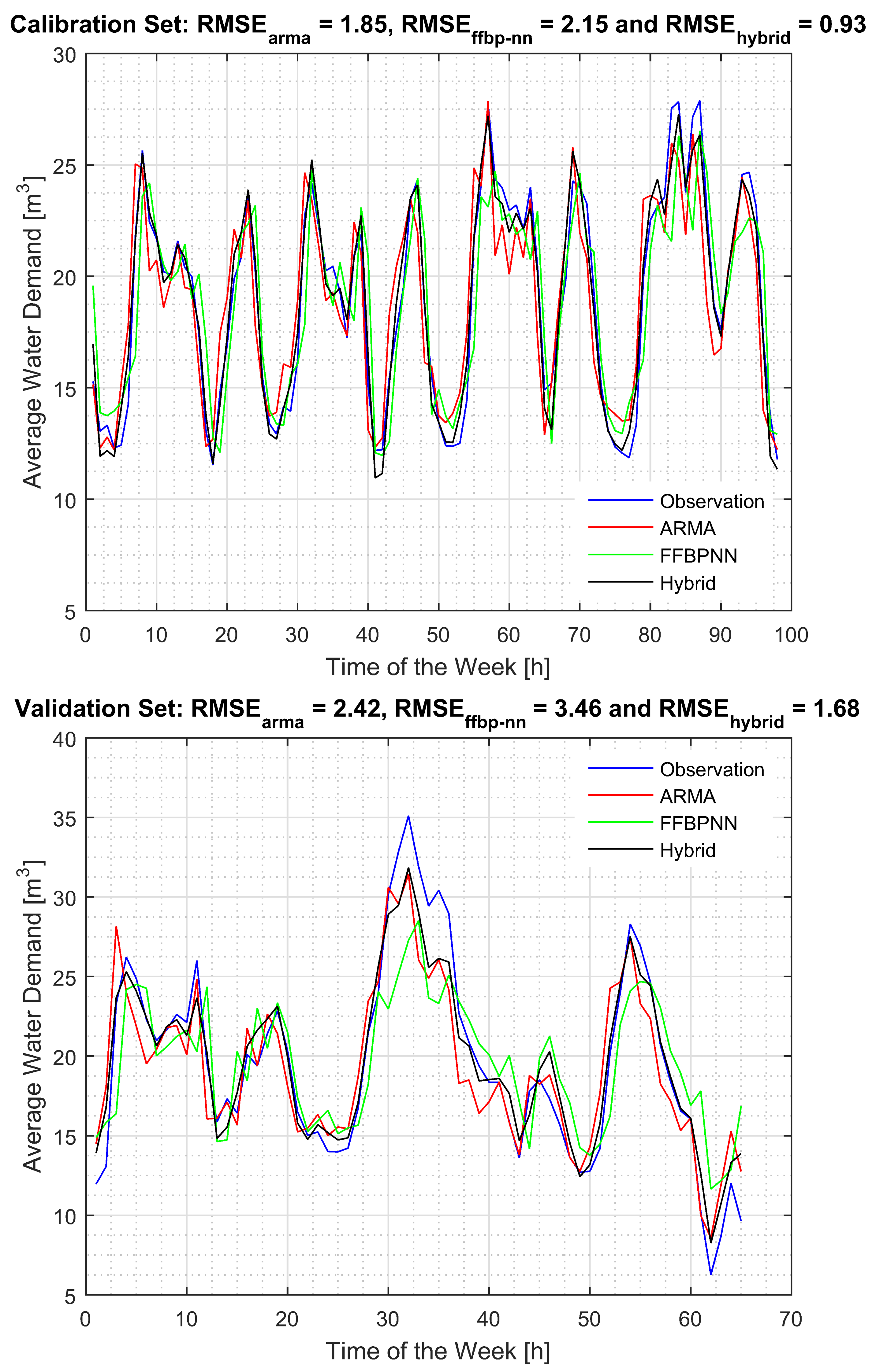
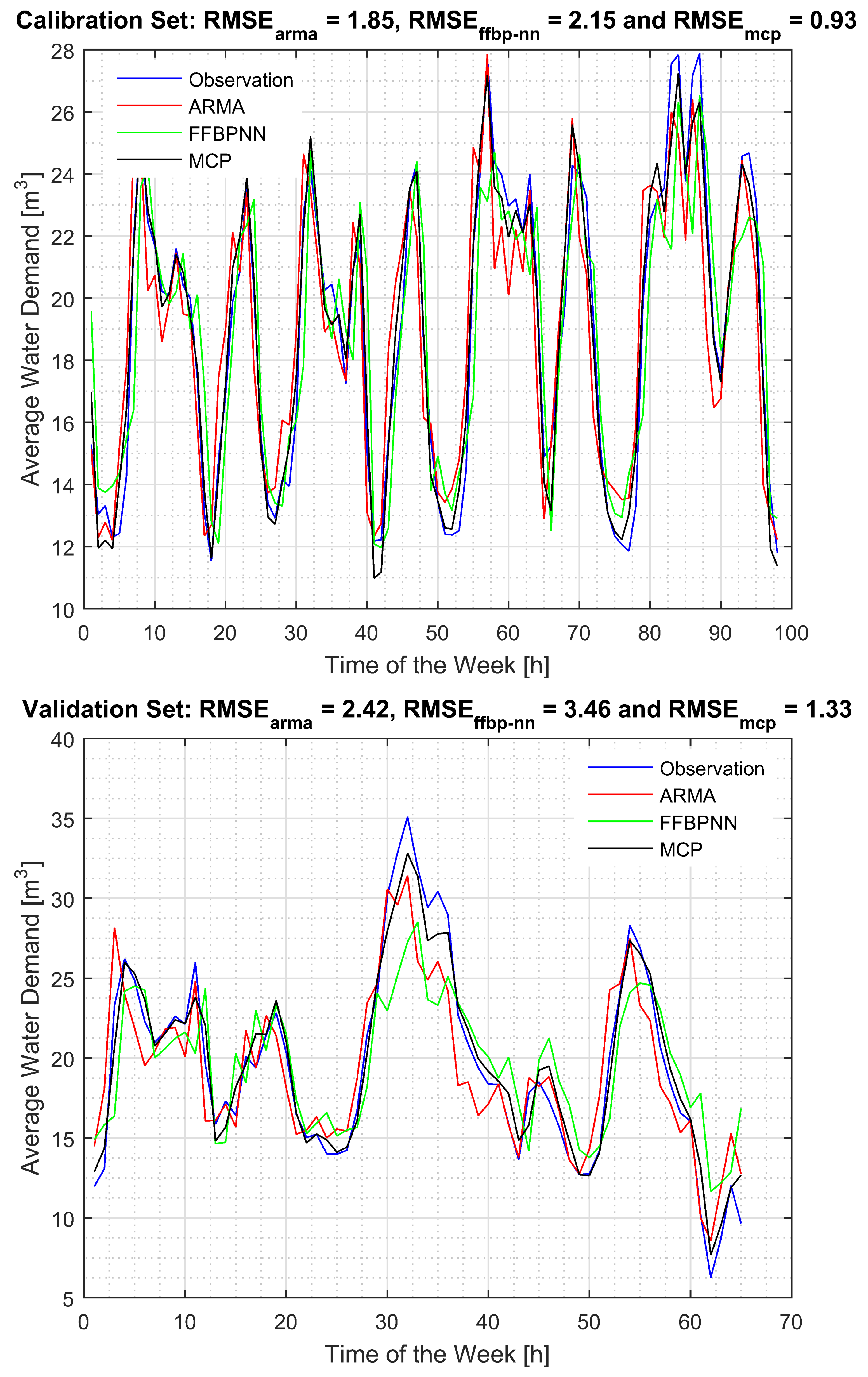
Figure 2, Figure 3 and Figure 4 and

Table 1. Performance Assessment: CAL and VAL mean the Calibration and Validation datasets.

	RMSE		MAPE (%)		NS Efficiency
	CAL	VAL	CAL	VAL	CAL	VAL
ARMA	1.852	2.418	8.318	10.288	0.841	0.844
FFBP-NN	2.151	3.462	9.027	15.700	0.786	0.681
Hybrid model	0.926	1.677	4.123	7.357	0.960	0.925
MCP	0.926	1.329	4.118	5.915	0.960	0.953

are obtained based on the MCP mathematical expressions given in Equations (1) and (2) together with the ARMA, FFBP-NN and hybrid models respectively given in Equations (3)–(5) [2]. In addition, the predictive performances of ARMA, FFBP-NN, hybrid model and MCP are evaluated by using the following forecasting statistical terms: root mean square error (RMSE), mean absolute percentage error (MAPE) and Nash-Sutcliffe (NS) model efficiency as given in Equations (6)–(8). Although optimising the single value statistics is not the main goal of this paper, the RMSE, MAPE and NS values presented in Table 1 show that MCP generated the best forecast compared to ARMA, FFBP-NN and hybrid model (see Figure 2 and Figure 3). In addition to providing the expected conditional forecast, as all the models do, the MCP approach allows the correct estimation of the full conditional predictive probability distribution (see Figure 4).

$$Y_t=\mu +\sum _{k=1}^p{\varphi }_k{Y}_{t-k}+{ϵ}_t+\sum _{k=1}^q{\theta }_k{\epsilon }_{t-k}$$

(3)

where p and q are the model orders, $\varphi$ is autoregressive parameter, $\theta$ is the moving average parameter, $\mu$ is the mean value of the process, and ${ϵ}_t$ is the forecast error at time t. $Y_t$ is the observed value of demand at time t, k is the number of historical periods, $Y_{t-k}$ and ${\epsilon }_{t-k}$ is the observation at time t − k [2].

$$Y_t={\alpha }_0+\sum _{j=1}^p{\alpha }_{j}f(\sum _{i=1}^h{\beta }_{ij}{Y}_{t-j}+{\beta }_{0j})+{ϵ}_t$$

(4)

where p is the number of hidden nodes, h is the number of input nodes, f is a sigmoid transfer function, ${\alpha }_j$ is the vector of the weights from the hidden to the output nodes, ${\beta }_{ij}$ are the weights from the input to hidden nodes, ${\alpha }_0$ and ${\beta }_{0j}$ are the weights of the arcs leaving from the bias terms [2].

$$\begin{array}{c}\hfill \widehat{Y_t}={\beta }_0+\sum _{i=1}^n{\beta }_i{\widehat{Y}}_{i,t}\end{array}$$

(5)

where ${\widehat{Y}}_{i,t}$ is the predicted value of the time series at time t using the $i_{th}$ model, ${\beta }_0$ is the regression intercept, ${\beta }_i$ coefficients are determined by optimisation or least squares regression to minimise the mean square error (MSE) between the hybrid forecast ${\widehat{Y}}_{i,t}$ and the actual data [2,7].

$$\begin{array}{c}MSE=\frac{1}{N}{\sum }_{t=1}^N{(Y_t-\widehat{Y_t})}^2\\ RMSE=\sqrt{MSE}\end{array}$$

(6)

$$MAPE=\frac{100}{N}\sum _{t=1}^N|\frac{Y_t-\widehat{Y_t}}{Y_t}|$$

(7)

$$NS=1-\frac{{\displaystyle \sum _{t=1}^N}{(Y_t-\widehat{Y_t})}^2}{{\displaystyle \sum _{t=1}^N}(Y_t-{\mu }_{Y_t}{)}^2}$$

(8)

where $Y_t$ is the real observation, $\widehat{Y_t}$ is the forecast value at time t, and ${\mu }_{Y_t}$ is the mean of real observation [2].

In Figure 4, the expected conditional value and a 95% probability band are compared to the observations showing that, as expected, most of the observations fall within the uncertainty band. The outcomes show that MCP provides more information in terms of a correct estimate of the full predictive probability density, which allows estimating the “expected utility function” within a Bayesian Decision scheme. In addition, the probability plots obtained in Figure 5 are generated based on [32], which shows the hypothesis that our predictive probability distribution correctly estimated cannot be rejected at the 95% probability level. The following tests (see Figure 5) demonstrate that MCP correctly estimates the predictive probability density, and such outcome is useful within the framework of water management procedures or to support decision-making [16,17,18,21]. Unlike the forecasts generated by ARMA, FFBP-NN and hybrid model, MCP provided a probabilistic forecast such that Equations (1) and (2) resulted to a mean and variance given below, where ${\widehat{y}}_1,{\widehat{y}}_2$ and ${\widehat{y}}_3$ are the model forecasts for ARMA, FFBP-NN and hybrid model respectively, and y is the historical observation.

According to Equations (1) and (2), which correspond to multiple regression in the Normal space, the predictive probability density of the predictand (the future demand) conditional to the three model predictions is the Normal probability density with:

$$\left\{\begin{array}{l}mean\left\{y\right|{\widehat{y}}_1,{\widehat{y}}_2,{\widehat{y}}_3\}={\mu }_y+\left[{\omega }_1{\omega }_2{\omega }_3\right]\left[\begin{array}{c}{\widehat{y}}_1-{\mu }_{{\widehat{y}}_1}\\ {\widehat{y}}_2-{\mu }_{{\widehat{y}}_2}\\ {\widehat{y}}_3-{\mu }_{{\widehat{y}}_3}\end{array}\right]\\ var\left\{y\right|{\widehat{y}}_1,{\widehat{y}}_2,{\widehat{y}}_3\}={\sigma }_y^2-\left[{\omega }_1{\omega }_2{\omega }_3\right]\left[\begin{array}{c}{\gamma }_{y{\widehat{y}}_1}\\ {\gamma }_{y{\widehat{y}}_2}\\ {\gamma }_{y{\widehat{y}}_3}\end{array}\right]\end{array}\right.$$

(9)

where ${\mu }_y$ and ${\sigma }_y^2$ are mean and variance of the predictand, while ${\mu }_{y_1}$, ${\mu }_{y_2}$ and ${\mu }_{y_3}$ are the means of the three models forecasts. The value of the weights ${\omega }_1,{\omega }_{2}and{\omega }_3$ can be estimated from the observations y (the predictand) and the model forecasts ${\widehat{y}}_1,{\widehat{y}}_{2}and{\widehat{y}}_3$ (the predictors), as:

$$\left[\begin{array}{c}{\omega }_1\\ {\omega }_2\\ {\omega }_3\end{array}\right]={\left[\begin{array}{ccc}{\gamma }_{{\widehat{y}}_1{\widehat{y}}_1}& {\gamma }_{{\widehat{y}}_1{\widehat{y}}_2}& {\gamma }_{{\widehat{y}}_1{\widehat{y}}_3}\\ {\gamma }_{{\widehat{y}}_2{\widehat{y}}_1}& {\gamma }_{{\widehat{y}}_2{\widehat{y}}_2}& {\gamma }_{{\widehat{y}}_2{\widehat{y}}_3}\\ {\gamma }_{{\widehat{y}}_3{\widehat{y}}_1}& {\gamma }_{{\widehat{y}}_3{\widehat{y}}_2}& {\gamma }_{{\widehat{y}}_3{\widehat{y}}_3}\end{array}\right]}^{-1}\left[\begin{array}{c}{\gamma }_{y{\widehat{y}}_1}\\ {\gamma }_{y{\widehat{y}}_2}\\ {\gamma }_{y{\widehat{y}}_3}\end{array}\right]$$

(10)

where ${\gamma }_{y{\widehat{y}}_i}$, $\forall i=1,\dots ,3$ are the co-variances between the observations y and the model forecasts ${\widehat{y}}_i$, while ${\gamma }_{{\widehat{y}}_i{\widehat{y}}_j}$, $\forall i,j=1,\dots ,3$ are the variances ($\forall i=j$) and the co-variances ($\forall i\ne j$) between the model forecasts.

By setting

$${\omega }_0={\mu }_y-\left[{\omega }_1{\omega }_2{\omega }_3\right]\left[\begin{array}{c}{\mu }_{{\widehat{y}}_1}\\ {\mu }_{{\widehat{y}}_2}\\ {\mu }_{{\widehat{y}}_3}\end{array}\right]$$

(11)

Equation (9) becomes:

$$\left\{\begin{array}{l}mean\left\{y\right|{\widehat{y}}_1,{\widehat{y}}_2,{\widehat{y}}_3\}={\omega }_0+\left[{\omega }_1{\omega }_2{\omega }_3\right]\left[\begin{array}{c}{\widehat{y}}_1\\ {\widehat{y}}_2\\ {\widehat{y}}_3\end{array}\right]\\ var\left\{y\right|{\widehat{y}}_1,{\widehat{y}}_2,{\widehat{y}}_3\}={\sigma }_y^2-\left[{\omega }_1{\omega }_2{\omega }_3\right]\left[\begin{array}{c}{\gamma }_{y{\widehat{y}}_1}\\ {\gamma }_{y{\widehat{y}}_2}\\ {\gamma }_{y{\widehat{y}}_3}\end{array}\right]\end{array}\right.$$

(12)

Accordingly, the estimated weights and variance become: ${\omega }_0=-2.285;{\omega }_1=0.406;{\omega }_2=0.349;{\omega }_3=0.370$ $var\left\{y\right|{\widehat{y}}_1,{\widehat{y}}_2,{\widehat{y}}_3\}=0.867$, leading to:

$$\{\begin{array}{l}mean\left\{y\right|{\widehat{y}}_1,{\widehat{y}}_2,{\widehat{y}}_3\}=-2.285+0.406{\widehat{y}}_1+0.349{\widehat{y}}_2+0.370{\widehat{y}}_3\\ var\left\{y\right|{\widehat{y}}_1,{\widehat{y}}_2,{\widehat{y}}_3\}=0.867\end{array}$$

(13)

In this work, following [32], we introduce the probability plot as a tool to assess the acceptance of the estimated probability. The probability plot is a plot of the estimated probabilities versus their empirical cumulative distribution function. For a perfect match, the shape of the resulting curve should be a 45 degree line corresponding to the cumulative uniform probability distribution. Alternatively, the curve will approach the bisector of the diagram. Kolmogorov confidence bands can be represented on the same graph as two straight lines, parallel to the bisector and at a distance dependent upon the chosen significance level of the test. For a 0.05 probability level, corresponding to a 95% band, the distance from the bisector line is $\frac{1.358}{\sqrt{n}}$, with n the number of observations used in the test. Figure 5 shows the probability plots relevant to the calibration and validation datasets. It is clear that the acceptability test for both datasets is passed at the 5% acceptance level, which implies that the developed predictive densities can be reliably used to estimate the expected utility values to be maximised in the Bayesian Decision scheme. Nonetheless, a better outcome could be obtained if a long record of data is used. Based on this study, the results presented in Figure 2, Figure 3, Figure 4 and Figure 5 and Table 1 show that MCP may be effectively used for real-time STWD forecast.

4. Conclusions

This paper intends to apply the MCP approach to demonstrate how a number of potential predictive models may improve our knowledge, and in turn estimate the predictive uncertainty (PU) when forecasting into the unknown future. To achieve this aim, comparative assessment of the forecasts generated using ARMA, FFBP-NN, hybrid model (i.e., combination of ARMA and FFBP-NN) and MCP conditional on ARMA, FFBP-NN and hybrid models is firstly conducted. Afterwards, the probability density of the future demand is built based on the forecasts generated by ARMA, FFBP-NN and the hybrid model. In addition, in this work, we demonstrate how to verify the correctness of the estimated predictive probability, which is an essential step towards correct expected losses estimates in view of decision making. The PU connected to the STWD forecast is estimated and validated based on $5\%$ probability acceptability test.

The results obtained show that the forecast generated by MCP marginally outperforms those of ARMA, FFBP-NN and hybrid model, and also allows assessment of the full predictive density to be used in the estimation of the expected losses in decision making. Finally, the probability acceptance/rejection tests on both the calibration and verification periods showed that the developed predictive densities are acceptable at $5\%$ probability level.

In conclusion, the outcomes of this study indicate that MCP may be efficiently used for real-time STWD prediction since it brings out the PU connected to the MCP forecast obtained, and with such information, water utilities could estimate the risk connected to a decision.

References

- Abu-Mahfouz, A.M.; Hamam, Y.; Page, P.R.; Djouani, K.; Kurien, A. Real-time dynamic hydraulic model for potable water loss reduction. Proc. Eng. 2016, 154, 99–106. [Google Scholar] [CrossRef]
- Anele, A.O.; Hamam, Y.; Abu-Mahfouz, A.M.; Todini, E. Overview, comparative assessment and recommendations of forecasting models for short-term water demand prediction. Water 2017, 9, 887. [Google Scholar] [CrossRef]
- Hamam, Y.; Brameller, A. Hybrid method for the solution of piping networks. Proc. Inst. Electr. Eng. 1971, 118, 1607–1612. [Google Scholar] [CrossRef]
- Billings, R.B.; Agthe, D.E. State-space versus multiple regression for forecasting urban water demand. J. Water Resour. Plan. Manag. 1998, 124, 113–117. [Google Scholar] [CrossRef]
- Adamowski, J.F. Peak daily water demand forecast modeling using artificial neural networks. J. Water Resour. Plan. Manag. 2008, 134, 119–128. [Google Scholar] [CrossRef]
- Qi, G.; Hamam, Y.; Van Wyk, B.J.; Du, S. Model-free prediction based on tracking theory and newton form of polynomial. World Acad. Sci. Eng. Technol. 2011, 5, 882–889. [Google Scholar]
- Donkor, E.A.; Mazzuchi, T.A.; Soyer, R.; Alan Roberson, J. Urban water demand forecasting: Review of methods and models. J. Water Resour. Plan. Manag. 2012, 140, 146–159. [Google Scholar] [CrossRef]
- Gharun, M.; Azmi, M.; Adams, M.A. Short-term forecasting of water yield from forested catchments after Bushfire: A case study from southeast Australia. Water 2015, 7, 599–614. [Google Scholar] [CrossRef]
- Pacchin, E.; Alvisi, S.; Franchini, M. A short-term water demand forecasting model using a moving window on previously observed data. Water 2017, 9, 172. [Google Scholar] [CrossRef]
- Brentan, B.M.; Luvizotto, E., Jr.; Herrera, M.; Izquierdo, J.; Pérez-García, R. Hybrid regression model for near real-time urban water demand forecasting. J. Comput. Appl. Math. 2017, 309, 532–541. [Google Scholar] [CrossRef]
- Candelieri, A. Clustering and support vector regression for water demand forecasting and anomaly detection. Water 2017, 9, 224. [Google Scholar] [CrossRef]
- Aly, A.H.; Wanakule, N. Short-term forecasting for urban water consumption. J. Water Resour. Plan. Manag. 2004, 130, 405–410. [Google Scholar] [CrossRef]
- Alvisi, S.; Franchini, M.; Marinelli, A. A short-term, pattern-based model for water-demand forecasting. J. Hydroinform. 2007, 9, 39–50. [Google Scholar] [CrossRef]
- Cutore, P.; Campisano, A.; Kapelan, Z.; Modica, C.; Savic, D. Probabilistic prediction of urban water consumption using the SCEM-UA algorithm. Urban Water J. 2008, 5, 125–132. [Google Scholar] [CrossRef]
- Caiado, J. Performance of combined double seasonal univariate time series models for forecasting water demand. J. Hydrol. Eng. 2009, 15, 215–222. [Google Scholar] [CrossRef]
- Todini, E. A model conditional processor to assess predictive uncertainty in flood forecasting. Int. J. River Basin Manag. 2008, 6, 123–137. [Google Scholar] [CrossRef]
- Coccia, G.; Todini, E. Recent developments in predictive uncertainty assessment based on the model conditional processor approach. Hydrol. Earth Syst. Sci. 2011, 15, 3253–3274. [Google Scholar] [CrossRef]
- Alvisi, S.; Franchini, M. Assessment of predictive uncertainty within the framework of water demand forecasting using the Model Conditional Processor (MCP). Urban Water J. 2017, 14, 1–10. [Google Scholar] [CrossRef]
- James, O.B. Statistical Decision Theory and Bayesian Analysis; Springer: New York, NY, USA, 1985; 617p, ISBN 0-387-96098-8. [Google Scholar]
- Bernardo, J.M.; Smith, A.F. Bayesian Theory; John Willey and Sons: Valencia, Spain, 1994. [Google Scholar]
- Bargiela, A. Managing uncertainty in operational control of water distribution systems. Integr. Comput. Appl. 1993, 2, 353–363. [Google Scholar]
- Barbetta, S.; Coccia, G.; Moramarco, T.; Todini, E. Case study: A real-time flood forecasting system with predictive uncertainty estimation for the Godavari River, India. Water 2016, 8, 463. [Google Scholar] [CrossRef]
- Reggiani, P.; Coccia, G.; Mukhopadhyay, B. Predictive uncertainty estimation on a precipitation and temperature reanalysis ensemble for Shigar Basin, Central Karakoram. Water 2016, 8, 263. [Google Scholar] [CrossRef]
- Todini, E. Flood forecasting and decision making in the new millennium. Where are we? Water Resour. Manag. 2017, 31, 3111–3129. [Google Scholar] [CrossRef]
- Gagliardi, F.; Alvisi, S.; Kapelan, Z.; Franchini, M. A probabilistic short-term water demand forecasting model based on the Markov Chain. Water 2017, 9, 507. [Google Scholar] [CrossRef]
- Raftery, A.E. Bayesian model selection in structural equation models. Sage Focus Ed. 1993, 154, 163. [Google Scholar]
- Krzysztofowicz, R. Bayesian theory of probabilistic forecasting via deterministic hydrologic model. Water Resour. Res. 1999, 35, 2739–2750. [Google Scholar] [CrossRef]
- Todini, E. Predictive uncertainty assessment in real time flood forecasting. In Uncertainties in Environmental Modelling and Consequences for Policy Making; Springer: Dordrecht, The Netherlands, 2009; pp. 205–228. [Google Scholar]
- Todini, E. The role of predictive uncertainty in the operational management of reservoirs. Proc. Int. Assoc. Hydrol. Sci. 2014, 364, 118–122. [Google Scholar] [CrossRef]
- Mardia, K.V.; Kent, J.T.; Bibby, J.M. Multivariate Analysis; Probability and Mathematical Statistics; Academic Press: London, UK, 1980. [Google Scholar]
- Herrera, M.; Torgo, L.; Izquierdo, J.; Pérez-García, R. Predictive models for forecasting hourly urban water demand. J. hydrol. 2010, 387, 141–150. [Google Scholar] [CrossRef]
- Laio, F.; Tamea, S. Verification tools for probabilistic forecasts of continuous hydrological variables. Hydrol. Earth Syst. Sci. Discuss. 2007, 11, 1267–1277. [Google Scholar] [CrossRef]
Figure 1.
Average water consumption for the 24 h of each day [2].
Figure 2.
STWD forecasts generated using ARMA, FFBP-NN and hybrid model.
Figure 3.
STWD forecasts generated ARMA, FFBP-NN and MCP.
Figure 4.
Calibration and Validation sets: MCP forecasts with estimated predictive uncertainties.
Figure 5.
Calibration and Validation sets: 5% probability acceptance limits for MCP prediction.