Effect of the Junction Angle on Turbulent Flow at a Hydraulic Confluence
by
 , , , , and
Nadia Penna
1,* ,
,
Mauro De Marchis
2,
Olga B. Canelas
3,
Enrico Napoli
4,
António H. Cardoso
3 and
Roberto Gaudio
1
1
Dipartimento di Ingegneria Civile, Università della Calabria, 87036 Rende, Italy
2
Dipartimento di Ingegneria Civile e Ambientale, Università degli Studi di Enna ‘Kore’, 94100 Enna, Italy
3
CERIS, Instituto Superior Tecnico, Universidade de Lisboa, 1649-004 Lisbon, Portugal
4
Dipartimento di Ingegneria Civile, Ambientale, Aerospaziale, dei Materiali, Università degli Studi di Palermo, 90133 Palermo, Italy
*
Author to whom correspondence should be addressed.
Water 2018, 10(4), 469; https://doi.org/10.3390/w10040469
Submission received: 17 February 2018
/
Revised: 1 April 2018
/
Accepted: 8 April 2018
/
Published: 12 April 2018
(This article belongs to the Special Issue Turbulence in River and Maritime Hydraulics)
Abstract
:Despite the existing knowledge concerning the hydrodynamic processes at river junctions, there is still a lack of information regarding the particular case of low width and discharge ratios, which are the typical conditions of mountain river confluences. Aiming at filling this gap, laboratory and numerical experiments were conducted, comparing the results with literature findings. Ten different confluences from 45 to 90 were simulated to study the effects of the junction angle on the flow structure, using a numerical code that solves the 3D Reynolds Averaged Navier-Stokes (RANS) equations with the k- turbulence closure model. The results showed that the higher the junction angle, the wider and longer the retardation zone at the upstream junction corner and the separation zone, and the greater the flow deflection at the entrance of the tributary into the post-confluence channel. Furthermore, it was shown that the maximum streamwise velocity does not necessarily increase with the junction angle and that it is not always located in the contraction section.
1. Introduction
A confluence is a geomorphological node where typically two upstream channels merge into a single downstream channel, giving rise to complex 3D flow patterns. By definition, the main stream is the longest of the two intersecting channels, whereas the tributary is the shortest. Considering that and are the discharge and the mean velocity of the upstream main channel, and and are the discharge and the mean velocity of the tributary channel, respectively, the discharge ratio between the two rivers () was defined by Best [1] as /. Similarly, the ratio between the tributary width () and the main channel width () is known as width ratio ().
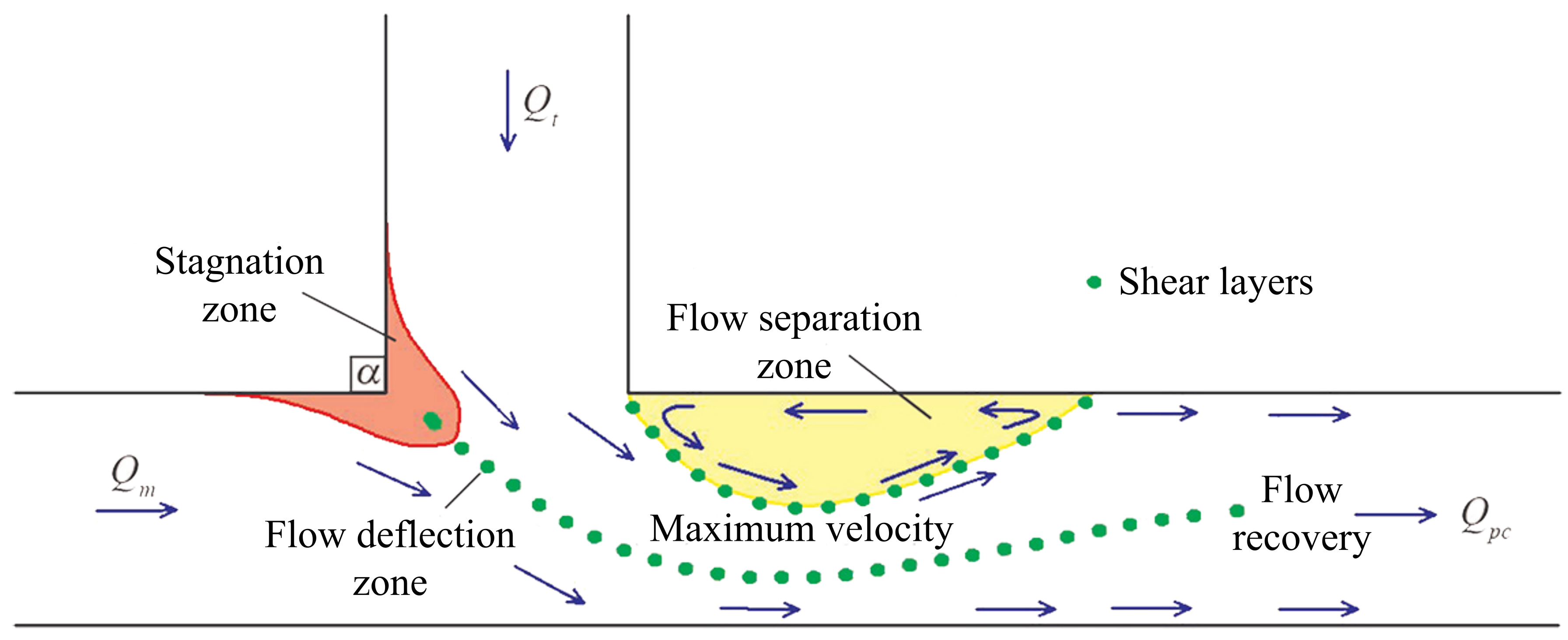
Although Taylor [2] was the first to study an asymmetrical channel confluence, proposing a 1D approach for the calculation of the water depth ratio between the upstream and downstream channels, the complete description of the flow field within a channel confluence is attributed to Best [1]. In fact, he distinguished six elements within a confluence (Figure 1): (1) a retardation zone at the upstream junction corner (commonly referred to as flow stagnation zone, even though it is characterized by reduced velocity that never decreases to zero); (2) a flow deflection zone, where each stream enters the confluence; (3) a flow separation zone, beyond the downstream junction corner; (4) an area of maximum velocity, located downstream of the confluence; (5) a flow recovery area, where the post-confluence flow tends to become unaffected by the confluence hydrodynamics; and (6) two main shear layers, caused by strong velocity gradients between the separation zone and the surrounding flow and between the flows coming from the tributary and main channels.
These zones depend, essentially, on the geometry (such as number of adjoining channels, cross-sectional area, junction angle , degree of concordance in elevation of the channel beds at the entrance to the confluence), flow and sediment parameters (such as between the two streams, bed material, sediment transport). The effects of these factors have been examined with both experimentally derived junctions in laboratory (e.g., [1,3,4]), and field investigations (e.g., [5,6,7,8,9]), recently integrated with numerical modelling (e.g., [10,11,12]). In particular, with laboratory experiments, it was possible to isolate and accentuate the effect of certain parameters and processes under controlled conditions, which then were varied by using numerical simulations in order to overcome limitations of the physical models.
Initially, focusing on the basic case of asymmetrical confluences with a fixed concordant bed and subcritical flow, most attention in the experimental campaigns found in the literature has been paid to determine relationships for the calculation of the flow depth or the energy loss at the junction (e.g., [13,14]). Subsequently, the determination of the shape and the extent of the separation zone has become the main objective of the research in the field of open-channel confluences, owing to its importance in (1) confining the effective width of the post-confluence channel towards the opposite wall of the junction, giving rise to the adjacent zone of maximum velocity and bed shear stress, and (2) in the overall head losses at junctions, as well as sediment and solute balances [15]. For instance, through vertical photography of surface dye traces, Best and Reid [16] showed that the width and length of the flow separation zone increases with both and the discharge ratio. Biron et al. [3] conducted a series of experiments in order to demonstrate the influence of the elevation of bed discordance on the characteristic zones of a confluence, with respect to the case of concordant beds. They showed that the difference in bed elevation destroys the flow deflection at the bed and creates a distortion of the mixing layer between the flows, resulting in fluid upwelling at the downstream junction corner. This phenomenon is responsible for the absence of a flow separation zone near the bed at the downstream junction corner and the lack of a zone of marked flow acceleration in the post-confluence channel. Gurram et al. [17], with their experimental work, yielded expressions for the pressure force on the lateral side walls, the ratio of flow depths in the junction point, the momentum correction coefficients, the extent of the separation zone determined with dye injections, and the lateral momentum contribution. They found that the separation zone increases with increasing values of Froude number (), and . Shumate [18] studied the general junction flow features occurring in a confluence. In particular, he found that the separation zone is larger near the surface, both in length and width. Moreover, up to a threshold, the separation zone lengthens as increases. Based on new confluence experiments, the detailed characteristics of the separation zone were analysed by Wang et al. [19] and Qing-Yuan et al. [20]. Specifically, Wang et al. [19] observed a zone of separation immediately downstream of the junction branch channel, the maximum and minimum velocity regions at the upstream and downstream in the confluent channel, and a shear plane developed between the two combining flows downstream of the confluent channel. Secondary circulations in different directions at the highest and lowest velocity zones were observed as well. Qing-Yuan et al. [20] used two different methods based on velocity streamlines and velocity isolines to investigate the geometry of the separation zone, which presented different forms with variations of distance to the flume bottom. Furthermore, they showed that the discharge ratio also influences the separation zone from bottom to surface. Also in the experiments of Biswa et al. [21], the width and the length of the flow separation zone increase with the contribution from the tributary channel to the discharge in the post-confluence channel (), while its shape remains practically unchanged. The most recent experimental campaigns were conducted separately by Schindfessel et al. [22] and by Birjukova et al. [23], investigating the time-averaged flow patterns in a confluence when largely exceeds [22] and in a confluence when largely exceeds [23]. In the first case, the separation zone was wider with respect to the literature reference cases, and a recirculating eddy appeared in the upstream main channel, confining the main channel incoming discharge and inducing a zone of reduced downstream momentum in its wake. Moreover, a new recirculation cell appeared with respect to the confluences studied by Gurram et al. [17] and Shumate [18], resulting in a change of sign of the lateral surface velocity near the bank opposite to the junction. Birjukova et al. [23] observed that, in their conditions, the separation zone limits the effective lateral flow cross-section, and hence results in the added acceleration of the mainstream flow near the downstream junction corner. Finally, Yuan et al. [24] analysed the distortion of the shear layer developed from the upstream junction corner at a open-channel confluence with a small width-to-depth ratio. They found that the distortion of the shear layer resulted in an increase in occurrence probabilities of ejection and sweep events within the shear layer, which were related to the turbulence presenting vortices induced by the wall.
In order to compare the experimental tests found in the literature, concerning laboratory asymmetrical confluences with fixed beds, Table 1 shows for each of them a brief overview of the geometrical and hydraulic conditions adopted. Moreover, it shows for each of the numerical simulations found in the literature: (1) the respective reference of the experimental tests used for the validation of the models and (2) the geometrical and hydraulic conditions.
In fact, using as a reference some of the experimental tests of Table 1 for the calibration of their models, several authors have performed Computational Fluid Dynamics (CFD) simulations to investigate detailed flow structures at confluences, changing the geometry, the hydraulic conditions or both. In particular, most of the CFD simulations have been conducted using the Reynolds Averaged Navier–Stokes (RANS) equations or Large Eddy Simulation (LES) models. For instance, the data of Biron et al. [3] were taken into account for the simulations of Bradbrook et al. [28] and Biron et al. [10]. Shakibainia et al. [29] used SSIIM 2.0, a RANS-based turbulent model, to reproduce the experiments of Shumate [18]. The same model and experimental test were used by Djordjevic [12] to study the effects of upstream planform curvature and bed elevation discordance between the tributary and main channels on the confluence hydrodynamics. However, Yang et al. [31], by using the commercial software FLUENT (ANSYS Inc., Canonsburg, PA, USA) and, again, the data of Shumate [18], showed how the adoption of dynamic meshes could give much higher accuracy than that of Volume of Fluid (VoF) or rigid lid method. The experimental tests of Birjukova et al. [23] were reproduced by Brito et al. [32], comparing the results obtained with different turbulence closure models for solving the RANS equations. More recently, Schindfessel et al. [33] used LES of the OpenFOAM suite to investigate the flow patterns for three different , considering the experimental tests by Schindfessel et al. [22]. They demonstrated that the tributary flow impinges on the opposing bank when the tributary flow becomes sufficiently dominant, causing a recirculating eddy in the upstream channel of the confluence, which induces significant changes in the incoming velocity distribution. The changed flow patterns also influence the mixing layer and the flow recovery. In their successive work, Schindfessel et al. [15] analysed the influence of the cross-sectional shape on the flow patterns in a confluence. They showed that the shape of the cross-section, and more particularly the geometry of the downstream corner, can induce lateral currents directed into the separation zone.
Despite the extensive research in hydrodynamic processes at junctions, it is evident how there is still a lack of information regarding channel confluences characterized by low discharge and width ratios. On a prototype scale, these conditions are characteristic of highly channelized mountain–river confluences and not common for low-land confluences, which, on the contrary, have inspired most of the literature studies on that topic [4,34]. Moreover, only a few studies have analysed the changes in the flow dynamics at a confluence as a function of the junction angle and all of them are referred to = 1, except the cases investigated by Gurram et al. [17] and Shakibainia et al. [29], for which the minimum value of was set equal to 0.33. Therefore, the research works in this field are not comprehensive and the extension of the existing knowledge to not yet explored conditions must be pursued.
In light of the above considerations, the paper describes the effects of the junction angle on the flow structure of a confluence with fixed concordant beds and both low width and discharge ratios, on the basis of the experimental campaign carried out by Birjukova et al. [23].
To this end, numerical simulations were initially carried out through the open-source numerical model known as PANORMUS (PArallel Numerical Open-souRce Model for Unsteady flow Simulation; [35]), available at www.panormus3d.org, which was adapted on purpose to the cases studied hereinafter. Then, the results of the numerical simulations were compared to the experimental data of Birjukova et al. [23] to validate the consistency of the model. Besides the original layout of the physical model, other nine layouts with different values from to were considered, in order to analyse their effects with particular attention paid to: (1) the extension of the retardation zone in the main and tributary channels; (2) the deflection of the tributary flow from the junction angle; (3) the length and width of the separation zone; and (4) the maximum streamwise velocity in the flow structure of the confluence.
Therefore, this study contributes to a better understanding of the flow processes occurring in a channel confluence, seeking to answer the following two main questions:
- What happens at low width and discharge ratios when junction angle is modified? How does this modification influence the flow dynamics?
- What do lower flow and width ratios imply with respect to the literature cases?
2. Description of Experiments and Simulations
2.1. Laboratory Flume: Set-up and Measurements
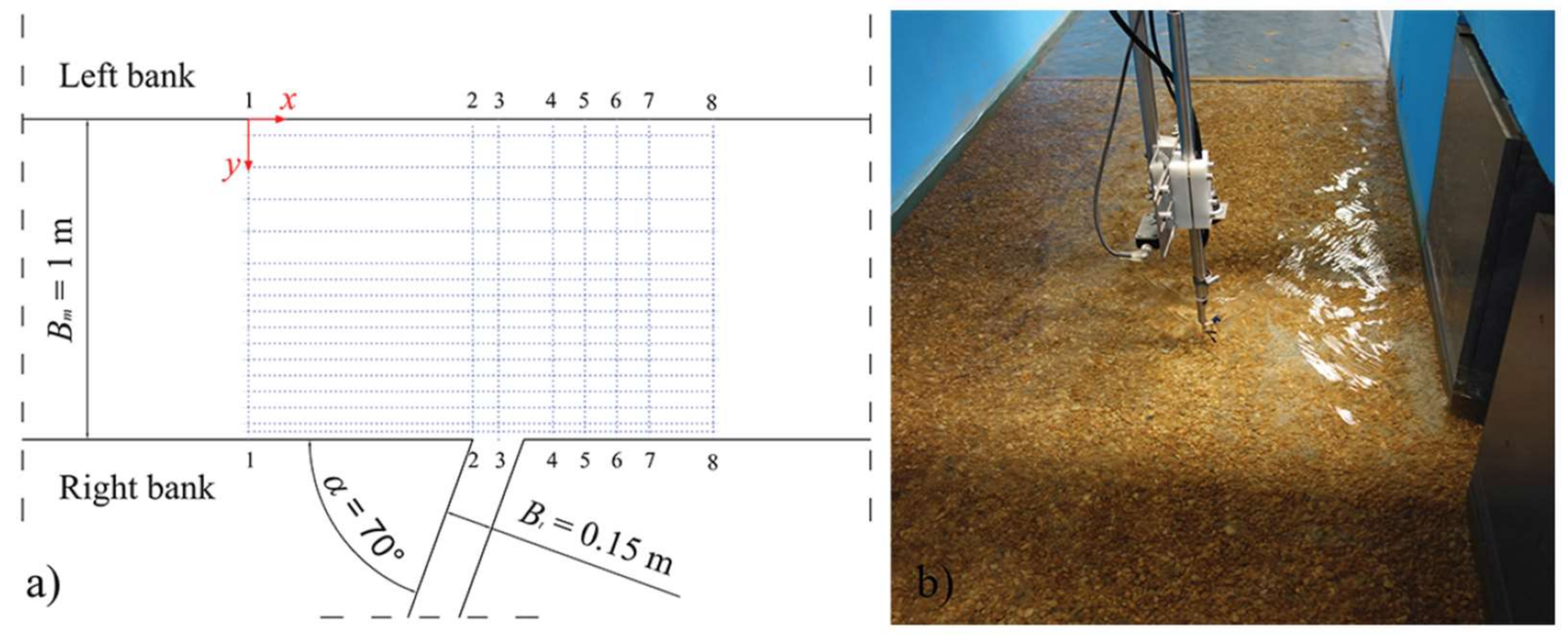
The experiment was conducted in the horizontal rectangular concrete flume of the Hydraulics Laboratory of the Instituto Superior Técnico (IST), Lisbon, Portugal (Figure 2a,b) as described in Birjukova et al. [23]. The length of the main and tributary channels were = 12 m and = 4.5 m, respectively, and the junction was located 5 m downstream of the inlet of the main channel, forming a confluence angle. The width of the main and tributary channels were = 1 m and = 0.15 m, respectively, resulting in a low equal to 0.15. Regarding the hydraulic conditions, the main channel discharge was set equal to = 0.044 ms, whereas the tributary one to = 0.005 ms, with = = 0.11 m, where is the main channel flow depth upstream the confluence and is the tributary flow depth. The discharge ratio, , assumes a low value equal to 0.114. To guarantee the development of a fully turbulent flow at cross-section no. 1 (Figure 2b), a layer of gravel (with = 6 mm) was placed on the channel bed.
An Acoustic Doppler Velocimeter (ADV), with a sampling frequency of 100 Hz and acquisition time per point equal to 90 s, was used to measure the flow field at the confluence, considering the sampling grid depicted in Figure 2a. In particular, the origin of the coordinate system is fixed at cross-section no. 1, 70 cm to the upstream junction corner at the left bank of the main channel. The horizontal axes x and y are directed in the streamwise and spanwise directions, respectively, whereas the vertical axis z, not shown in Figure 2a, starts at the bottom and is directed towards the water free surface. As many as 128 vertical profiles were considered in this study: eight cross-section and 16 lateral positions, starting at 2.5 cm from the right wall of the main channel, with a step of 5 cm from y = 0.05 m to 0.55 m and of 10 cm from y = 0.55 m to 0.95 m. Each profile is constituted by 18 measuring points (i.e., 11 points at a vertical displacement of 2 mm in the lower ≈ 30% of the flow depth and seven points with a step of 7 mm in the upper flow region). Note that no velocity measurements were undertaken in the tributary channel.
2.2. Analysis of the Experimental Data
The analysis of the experimental data is a crucial aspect for the correct interpretation of the results obtained with numerical simulations. In fact, the consistency of the model is evaluated on the basis of this preliminary investigation, which reveals the actual flow pattern found in the laboratory confluence.
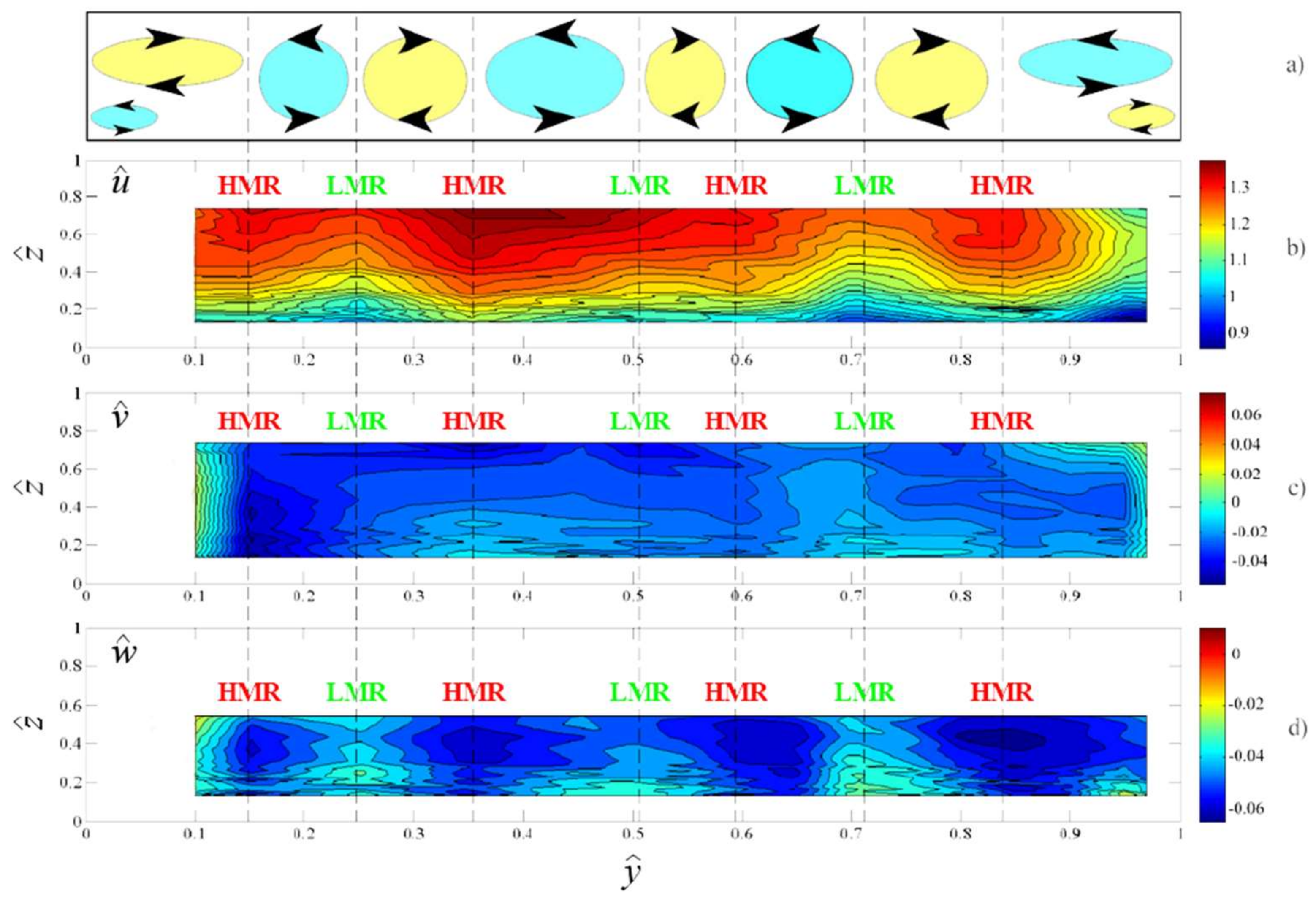
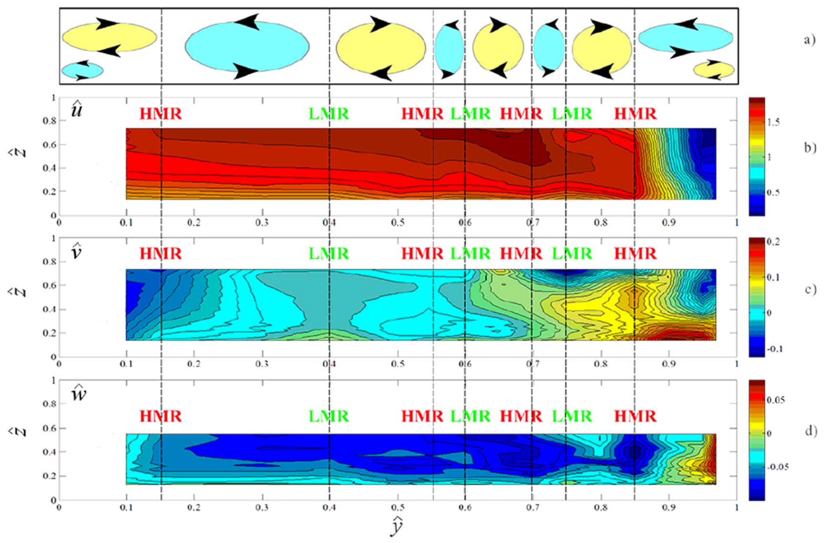
The time-averaged components of the velocity vector (, , , in the streamwise, spanwise and vertical directions, respectively) measured at cross-section no. 1, normalized with the mean flow velocity upstream to the confluence ( = /(B ) = 0.38 ms) are shown in Figure 3, where is defined as y/ and as z/. Specifically, was used as a reference, even though, from the analysis of the ADV data, a mean velocity equal to 0.41 ms was obtained, with a relative error with respect to equal to . This difference can be attributed to the fact that the ADV measurements do not cover the entire width and depth of the channel, along cross-section no. 1.
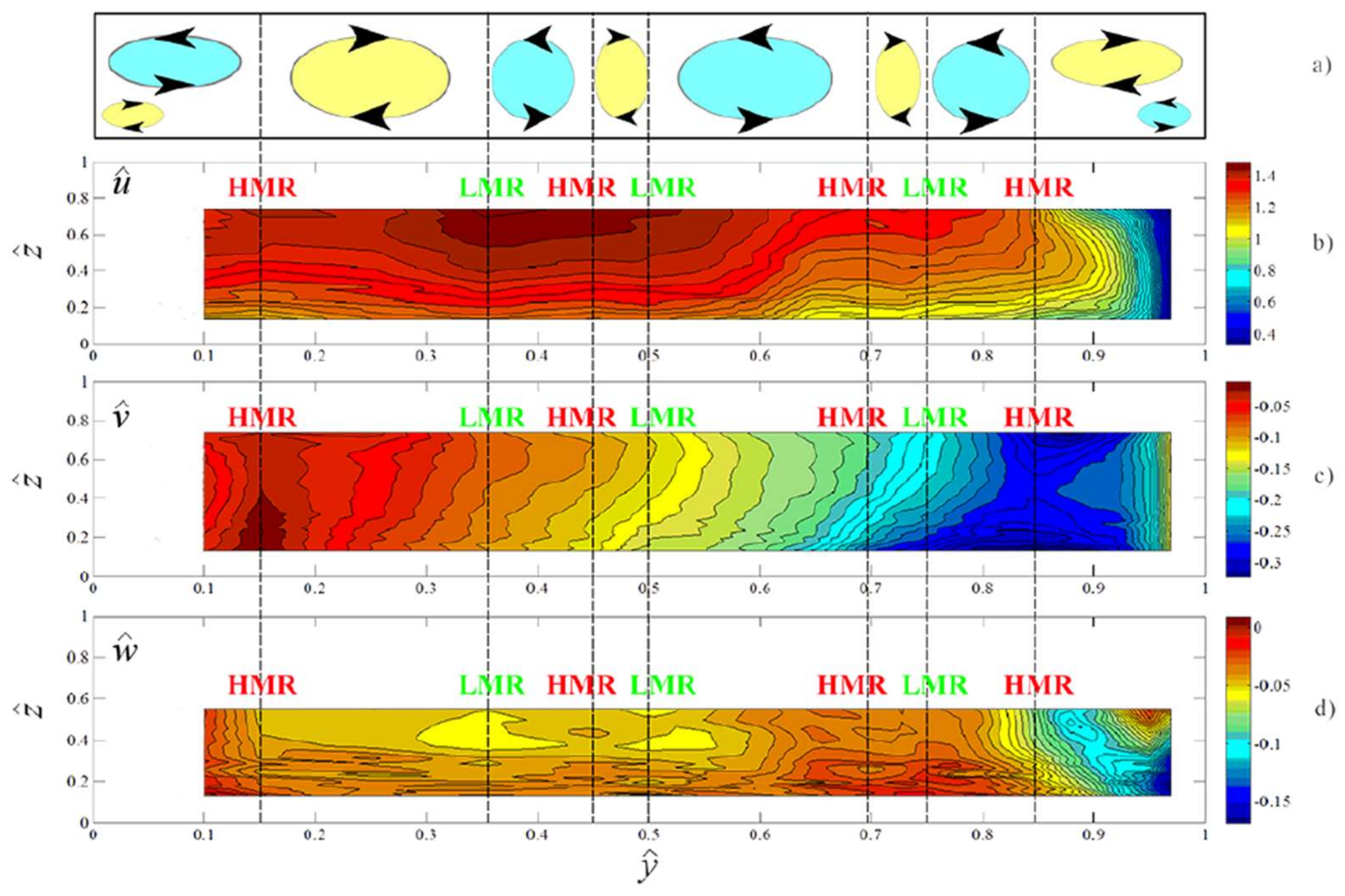
The analysis of such patterns reveals the presence of a comparatively strong secondary currents over the entire width of the cross-section (Figure 3a), even if, as the experiment was designed with an aspect ratio / = 8.8, either a weak or inexistent secondary circulation pattern would be expected in the central region of the channel. The reason behind the existence of such strong heterogeneity in Figure 3b derives, essentially, from a combination of two processes. In fact, near the lateral walls, the presence of the secondary currents is due to the amplification of the surface-corner vortex caused by the difference in roughness between the bank and the bed [36,37], whereas, along the width of the main channel, the turbulent secondary flows are attributed to the spanwise heterogeneity in roughness height, which causes low-momentum regions (LMRs) spanwise-adjacent to high-momentum regions (HMRs) (their spanwise positions are labelled in Figure 3). In fact, the layer of gravel was not uniformly glued on the channel bed and, therefore, different topographical scales were arranged in a highly irregular manner. Several studies showed how the formation of these vortical structures are influenced by the roughness height (e.g., [38,39,40]). In general, the identified LMR and HMR patterns tend to occur at spanwise locations of recessed and elevated roughness (relative to the mean elevation), respectively, with the swirling motions residing at spanwise locations of intense spanwise gradients in topographical height [39]. The same trend could be recognized in the other cross-sections (see Figure 4 and Figure 5).
2.3. Computational Domain and Validation of the Numerical Model
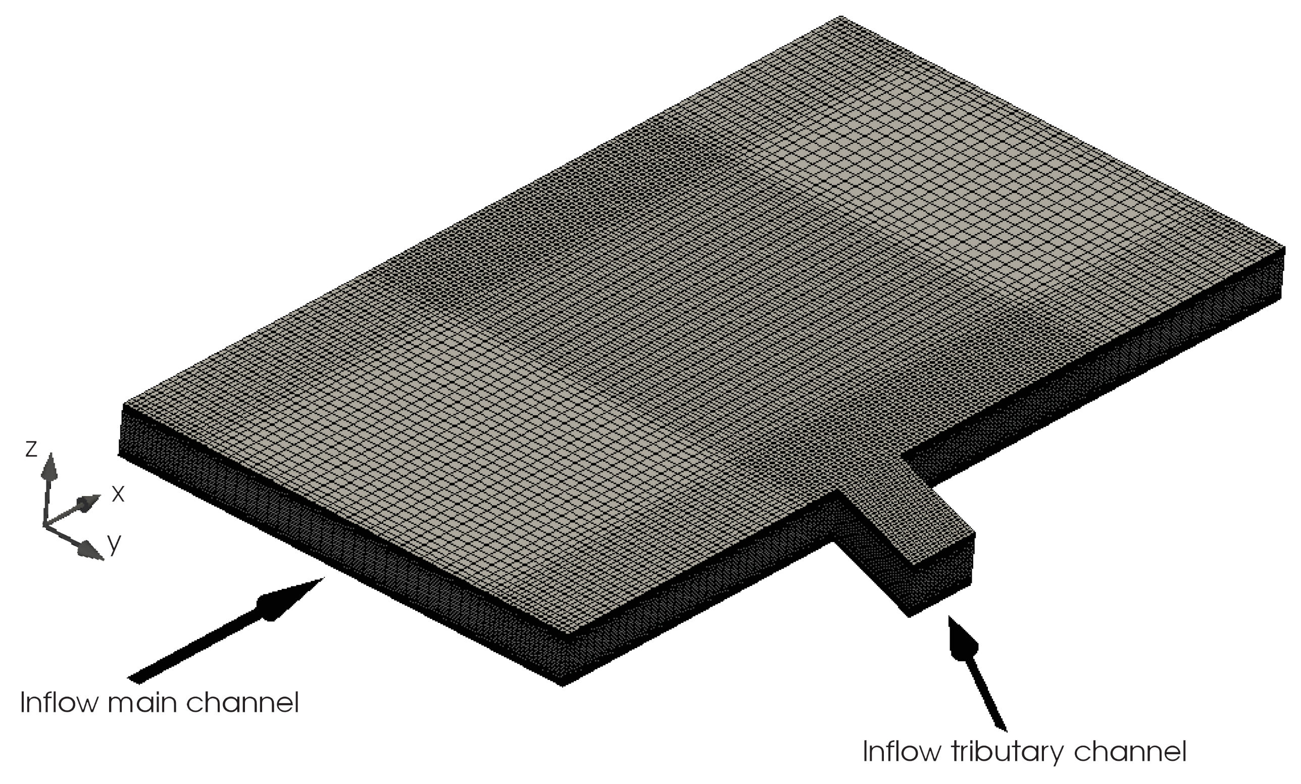
The numerical simulations have been carried out by using the finite-volume numerical code PANORMUS (second-order accurate both in time and space). It solves the 3D RANS equations with the k- turbulence closure by using a finite-volume method on a three-dimensional, non-orthogonal, structured grid. For the time advancement of the solution, the numerical model uses the explicit Adams–Bashforth method, whereas to overcome the pressure-velocity decoupling, typical of incompressible flows, the fractional-step technique is employed. The predictor–corrector system is solved through the Line Successive OverRelaxation method (L-SOR) algorithm. For details on the numerical model and the mathematical formulation of the RANS equations, see [41]. The model is resolved in a computational domain reproducing the experimental laboratory facility. Specifically, the length of the tributary was determined arbitrarily because no velocity measurements were available from the experimental campaign, which would be used to validate the numerical results in the tributary. The confluence domain, after a grid sensitivity analysis, was discretized in 128 × 96 × 32 cells in the streamwise, spanwise and vertical directions, respectively, by using a MATLAB (The MathWorks, Inc., Natick, MA, USA) code programmed on purpose. This resolution was selected so that the implementation of a finer grid did not show a considerable difference in the results. The mesh was refined near the walls and in the confluence zone (Figure 6), in order to obtain a finer discretisation close to the momentum transfer regions and the boundaries. A non-uniform grid was also used in the vertical direction, which was refined near the bottom and near the free-surface (imposed at 0.114 m above the bottom). The computational resolution is fine enough to reproduce the experiments and give a new insight into the dynamics of the channel confluence.
Both in the main and tributary channels, the flow is driven with assigned inflow conditions. Specifically, at the inlet of the two channels, a mean velocity profile is imposed to achieve the same values of flow rate and as in the experimental channel by means of a centrifugal pump. The logarithmic law of the wall was used near the solid boundaries (lateral walls and bottom) and null derivatives for all variables and hydrostatic pressure distribution were prescribed at the outflow boundary (Neumann-type boundary conditions). At the upper boundary, the free slip condition was adopted, which is justified as the tested numbers (defined with the flow depth and mean velocity in the incoming and downstream channels) were smaller than 0.5 [11]. At the bottom wall, an equivalent roughness height of 3 mm (thus, lower than ) was considered for all simulations, in order to take into account the difference in roughness between the vertical walls and the channel bed. Such value was verified successively to be acceptable by comparing the experimental and numerical data.
The measured flow field at cross-section no. 1 and were used to calibrate the inflow in the main channel, whereas, for the tributary, only was taken into account.
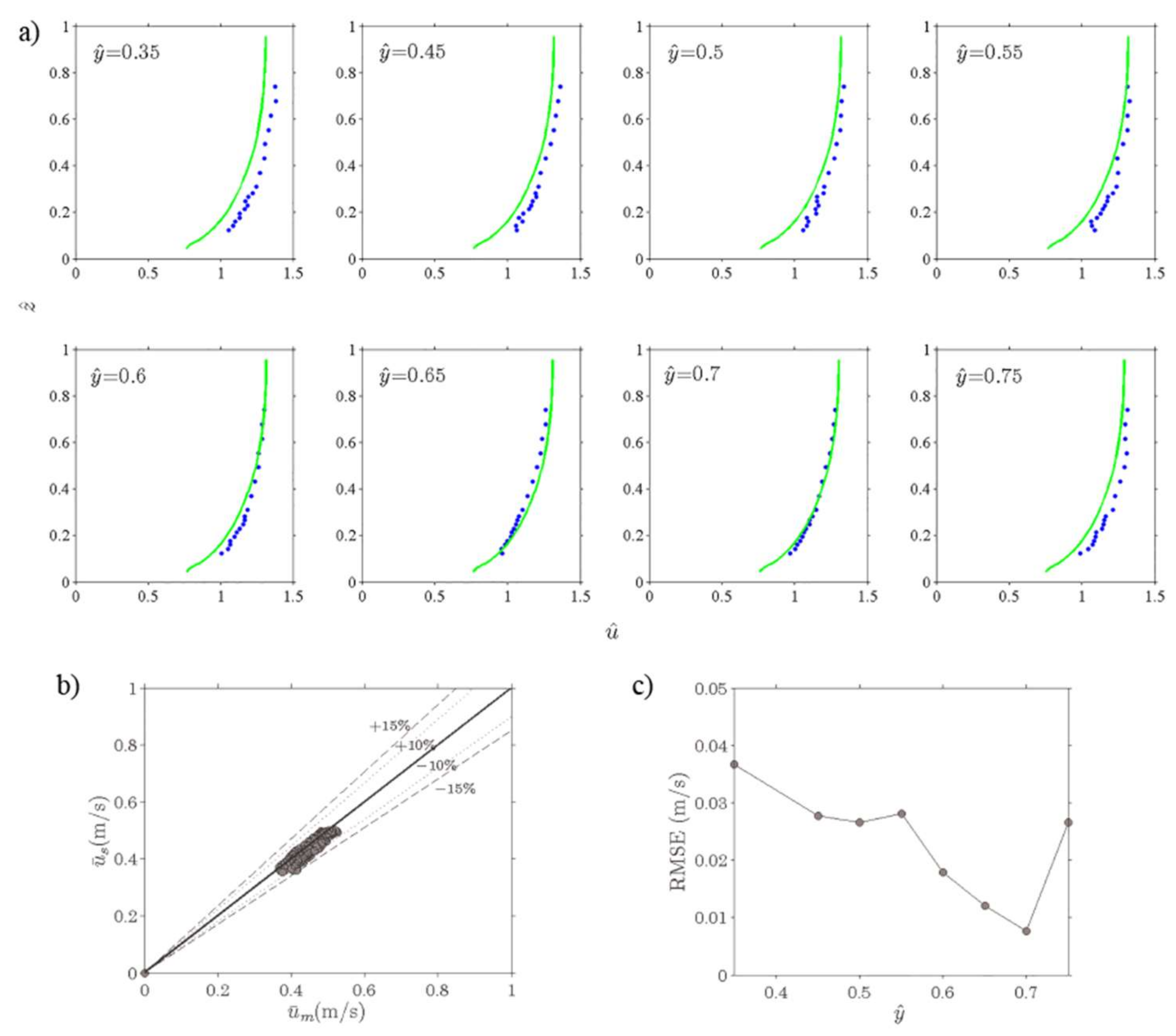
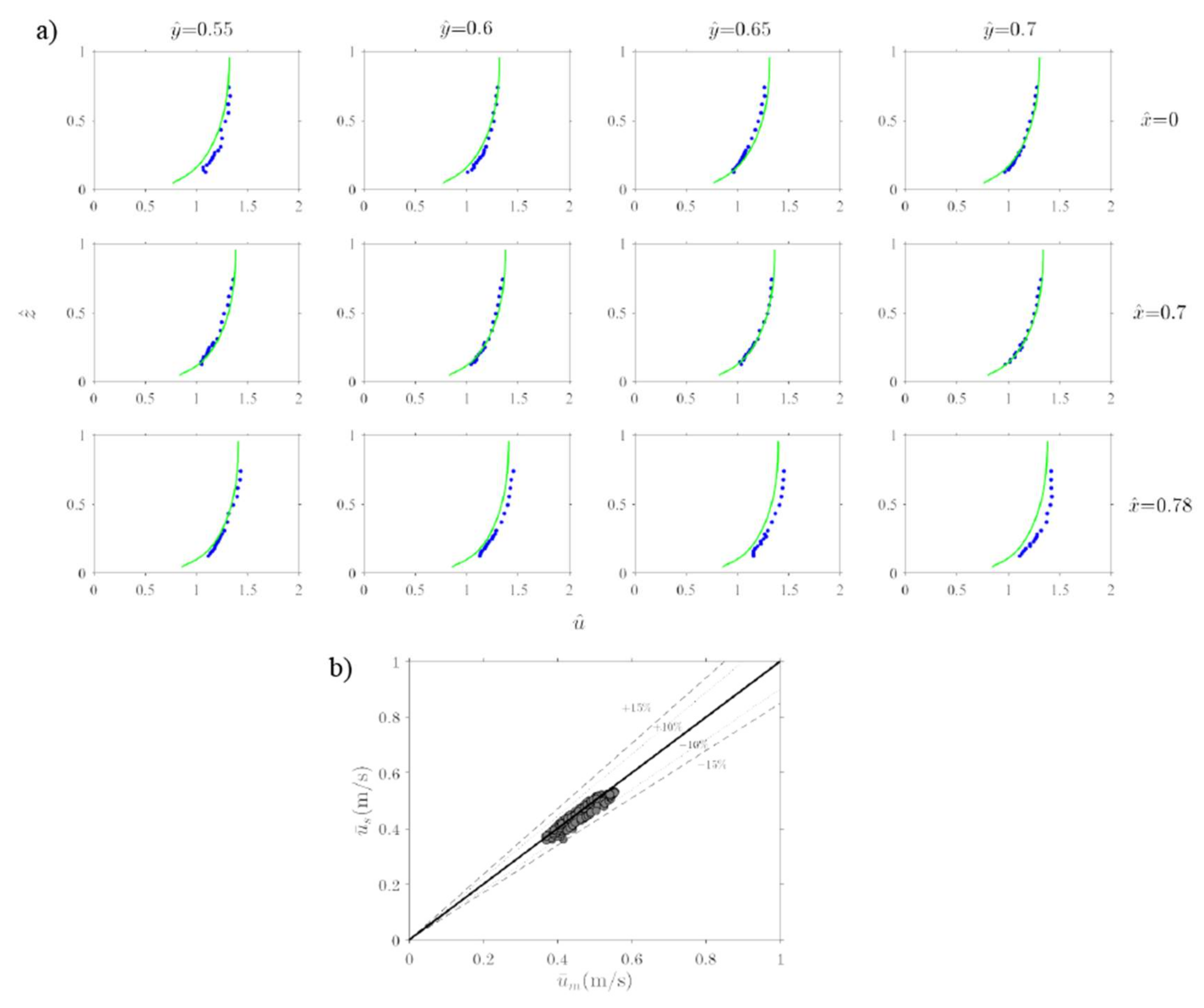
Figure 7a shows the comparison between the measured and the simulated velocity profiles of the non-dimensional streamwise component at eight lateral positions along cross-section no. 1. Despite the presence of secondary currents, the results obtained with PANORMUS demonstrated a satisfactory agreement between the experimental and numerical data in the central part of the main channel (from = 0.35 to = 0.75). Here, the major discrepancies occurred in the lower part of the velocity profiles, near the bottom, where the velocity values were slightly underestimated owing to the use of the wall function.
To quantify such discrepancies, Figure 7b shows the matching between measured () and simulated () streamwise velocity components, from = 0.35 to = 0.75, with the perfect agreement line and the and bands. It is evident that the maximum deviation is confined between and . Moreover, Figure 7c shows the Root Mean Square Error (RMSE) obtained for each velocity profile and calculated as , where N is the total number of measurement points along the vertical direction.
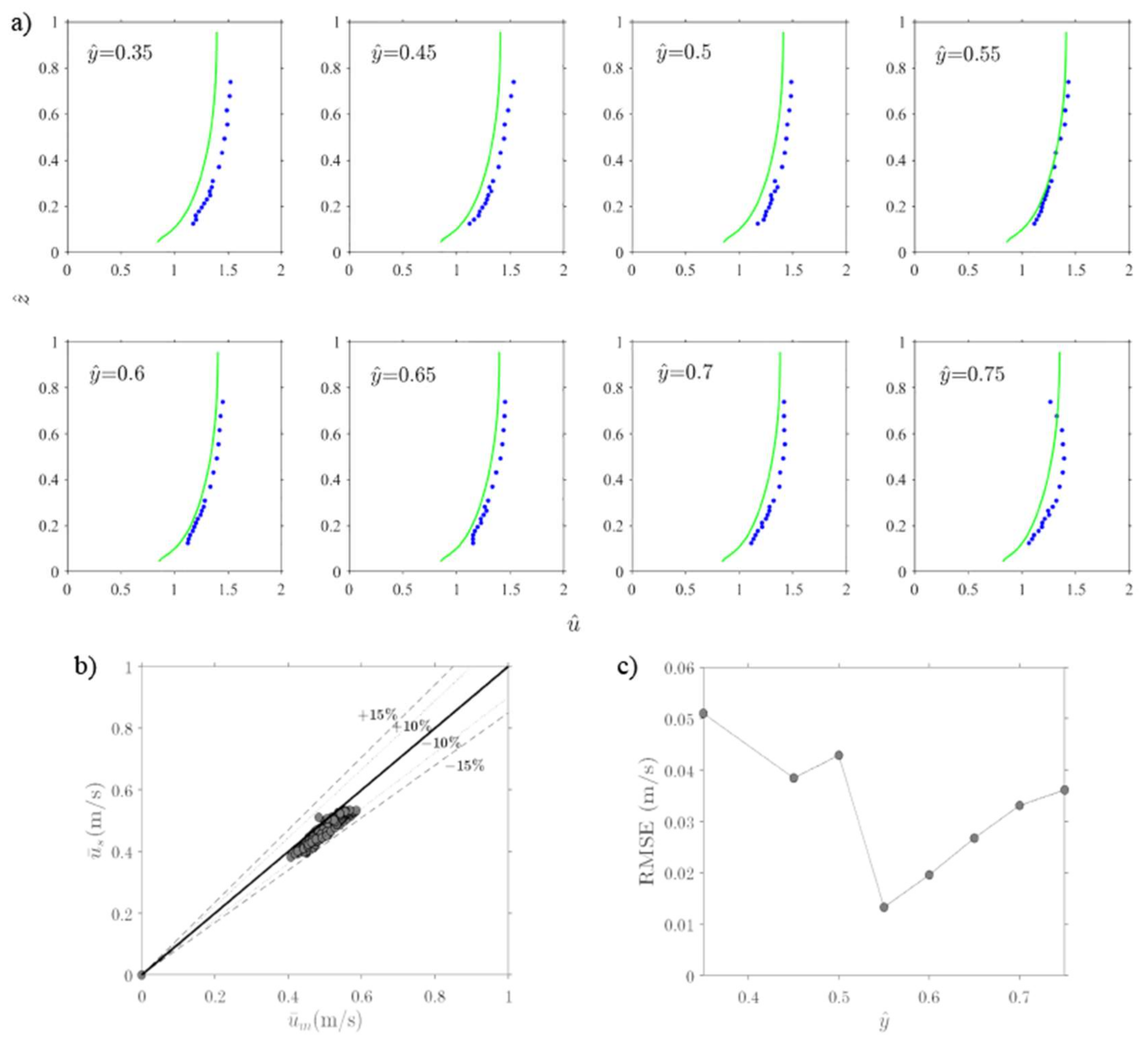
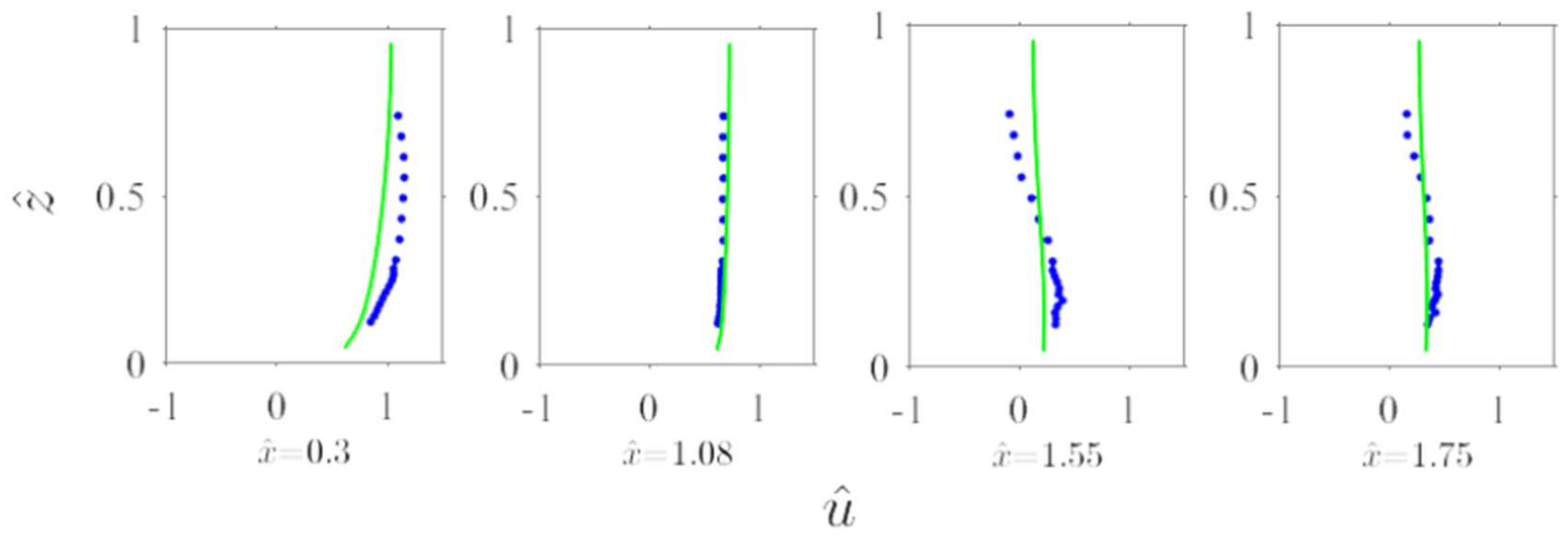
Figure 8 and Figure 9 show the same comparisons along cross-section no. 3, in correspondence of the tributary channel, and along four different longitudinal profiles. It is clearly visible that the maximum deviation, in both cases, is generally confined between and .
However, it is important to highlight that, near the internal wall, where strong flow recirculation occurs, differences in measured and estimated values were detected (as an example, see Figure 10). This behaviour was not unexpected. In fact, similar deviation in the separation zone was shown in other literature studies (i.e., [29,42]), using different experimental data and numerical models.
For this reason, the model was also validated considering the shape of the separation zone in terms of its length () and width ().
Different techniques were employed in the past for accurately determining the separation zone (e.g., [15,20]). However, since this is a region of decreased downstream momentum, the delineation of the separation zone extension is not an easy task. Generally, for a given z coordinate, the length of the separation zone is defined as the distance from the downstream corner of the junction to the reattachment point. In addition, according to the boundary layer theory, the separation zone starts when the velocity near the wall is zero or negative. Therefore, the general hypothesis that considers the downstream junction corner as the starting point of the separation zone (known as the separation point) is misleading. Especially in the case of low angles, it is expected that the flow arriving from the tributary channel tends to adhere to the wall downstream of the confluence and, only when the flow velocity can no longer overcome adverse pressure gradient, flow separation occurs. Therefore, the separation point is not coincident with the downstream junction corner, but it is located downstream of it.
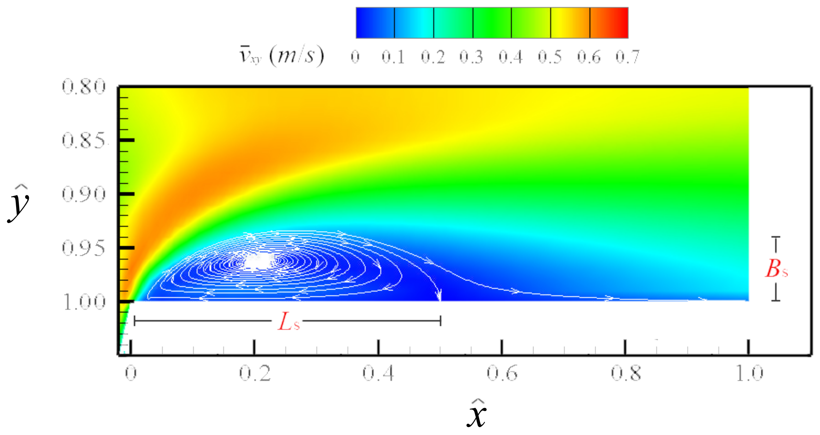
Specifically, the separation zone was delimited by the streamlines shown in Figure 11, where the time-averaged velocity in the horizontal plane was plotted. was defined as the distance from the separation point to the reattachment point, whereas was the distance from the wall to the point belonging to the streamline passing through the reattachment point, in which is null.
For = 70, and were 48.6 cm and 6.4 cm, respectively. These two main features were also obtained from the experimental data and were approximately 46 cm and 6 cm, respectively, showing that the numerical model slightly overestimates with a relative error equal to . The error is greater for and is equal to , since the predicted width is narrower than the measured one. This discrepancy can be attributed to the effect of the secondary currents, discussed in Section 2.2. Such results were compared with those obtained by Brito et al. [32], who modelled the free surface with the VoF method. In particular, they obtained the following separation zone characteristic sizes: = 54 cm and = 8.7 cm. Therefore, the estimations of both and are more precise in the present study, with respect to that of Brito et al. [32].
3. Results and Discussion
To study the effects of the junction angle on the flow structure of a confluence with fixed concordant beds and low width and discharge ratios, the computational domain created on the basis of the facility used by Birjukova et al. [23] was modified according to nine other different junction angles, ranging from to with a step of .
The simulations were carried out using the same of the experimental test in order to compare the obtained results as a function of solely , maintaining constant hydraulic conditions for both channels. The modification of the junction angle implies the change of the constant mass force (per unit mass) that drives the flow into the tributary. Such value is just the slope of the tributary towards the main channel. Therefore, to always guarantee the same value of , preliminary and separate simulations of fully developed turbulent flows were performed adapting the constant mass force to each simulated geometry. The main channel flow, upstream to the confluence, was not affected by the changes of the junction angle.
The results are presented by comparing the effects of the junction angle on the retardation zone, the flow deflection zone, the flow separation zone and the maximum streamwise velocity zone. Although these regions are strongly related, hereinafter they are analyzed independently for a better understanding of each involved hydrodynamic process.
3.1. Retardation Zone
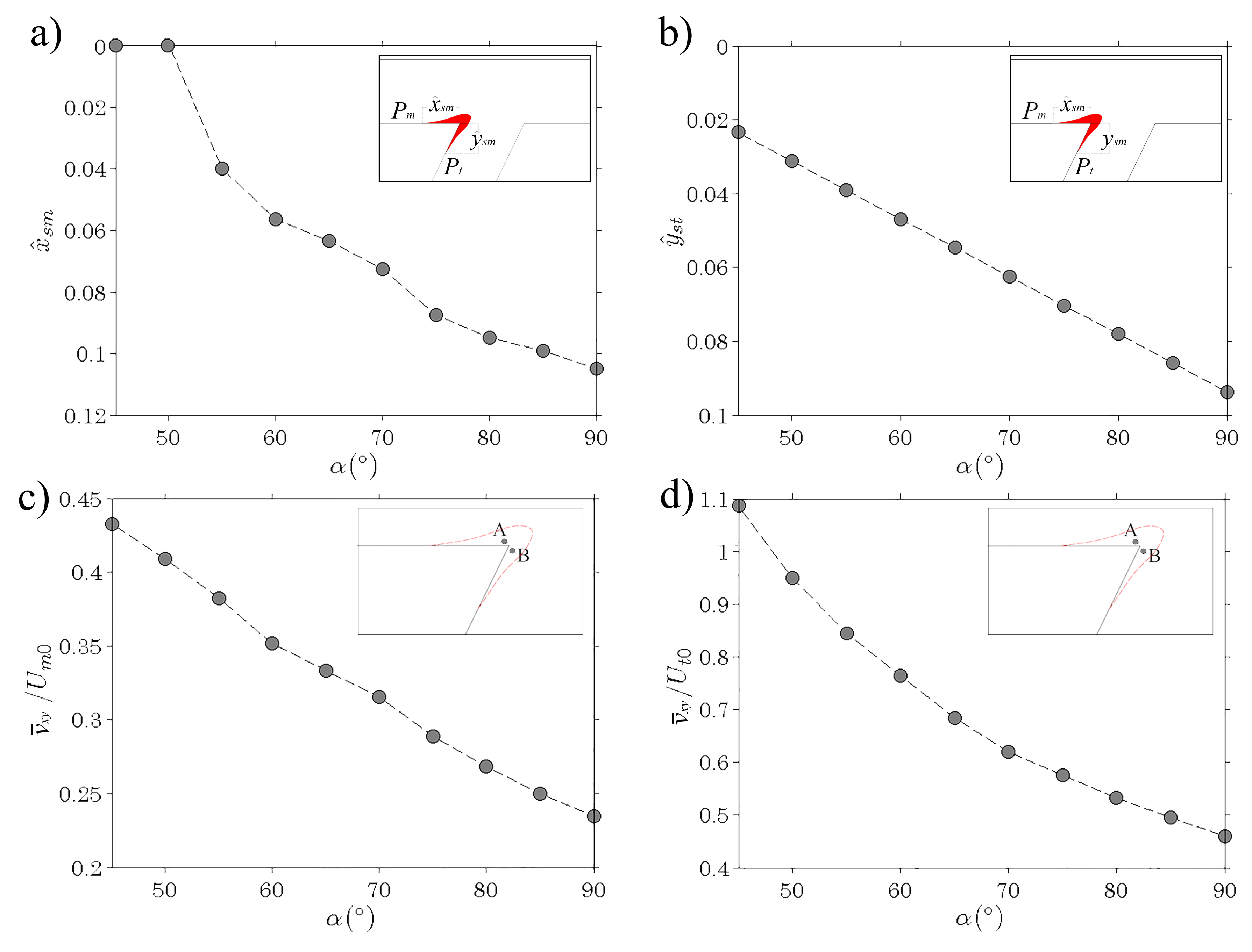
The retardation zone within each channel originates from the deflection of flows away from the upstream junction corner. It is a region of reduced velocities, whose size depends on the junction angle. Two particular points, for each of the two incoming channels, characterize this zone and were identified in this work by the respective distances from the upstream junction corner to the points in which the velocity vector deflects from the wall with an angle greater than (points and , respectively, in the main and tributary channels) (Figure 12a,b). In particular, is the streamwise distance between the upstream junction corner and the point , while is the lateral distance between the upstream junction corner and the point .
Figure 12a,b shows such values made non-dimensional with for different angles at elevation . It is possible to note that, as increases, and increase quasi-linearly, causing a more extended retardation zone. In addition, for equal to and , the retardation zone is confined only within the tributary channel, since is equal to 0. The maximum extension of such region occurs at , where and are about 0.1 m and 0.09 m, respectively.
Therefore, the higher the junction angle, the more extended the retardation zone and the lower the velocities in this region. In fact, as an example, Figure 12c,d shows the relative flow velocity at points A and B located immediately upstream to the junction corner within the main and tributary channels, respectively, and their variation with the confluence angle. The relative flow velocity at point A is expressed as , where at point A. The relative flow velocity at point B is expressed as , where at point B and is the mean velocity of the tributary channel (equal to 0.29 ms). It is evident that the flow retardation rate increases at a higher junction angle, since, increasing , a progressively strong retardation of the flow velocity is observed in both the channels.
The results are consistent with the findings of several researchers (e.g., [1,13,18]), who, however, focused on the position of a stagnation point only within the tributary channel. Actually, as it was observed in this work, two particular points in the two incoming channels can be taken into account to delimit the extension of the retardation zone. However, they can not be defined as stagnation points since the velocity in that points is not equal to zero.
3.2. Flow Deflection Zone
As Gurram et al. [17] observed, assuming that the inflow angle along the junction cross-section is equal to the junction angle is a wrong hypothesis. In fact, the lateral inflow velocity varies from the upstream to the downstream junction corners, increasing towards this latter, as it occurs in curve flow, but always with a smaller angle with respect to . To measure the deflection of the flow on the horizontal plane at the tributary entrance into the confluence, the flow angle was calculated, along the entire cross-section connecting the upstream and downstream junction corners, on the basis of the streamwise and spanwise time-averaged components of the velocity vector: = arctan(/). Then, the angle of deflection was made non-dimensional by dividing by , giving the new variable .
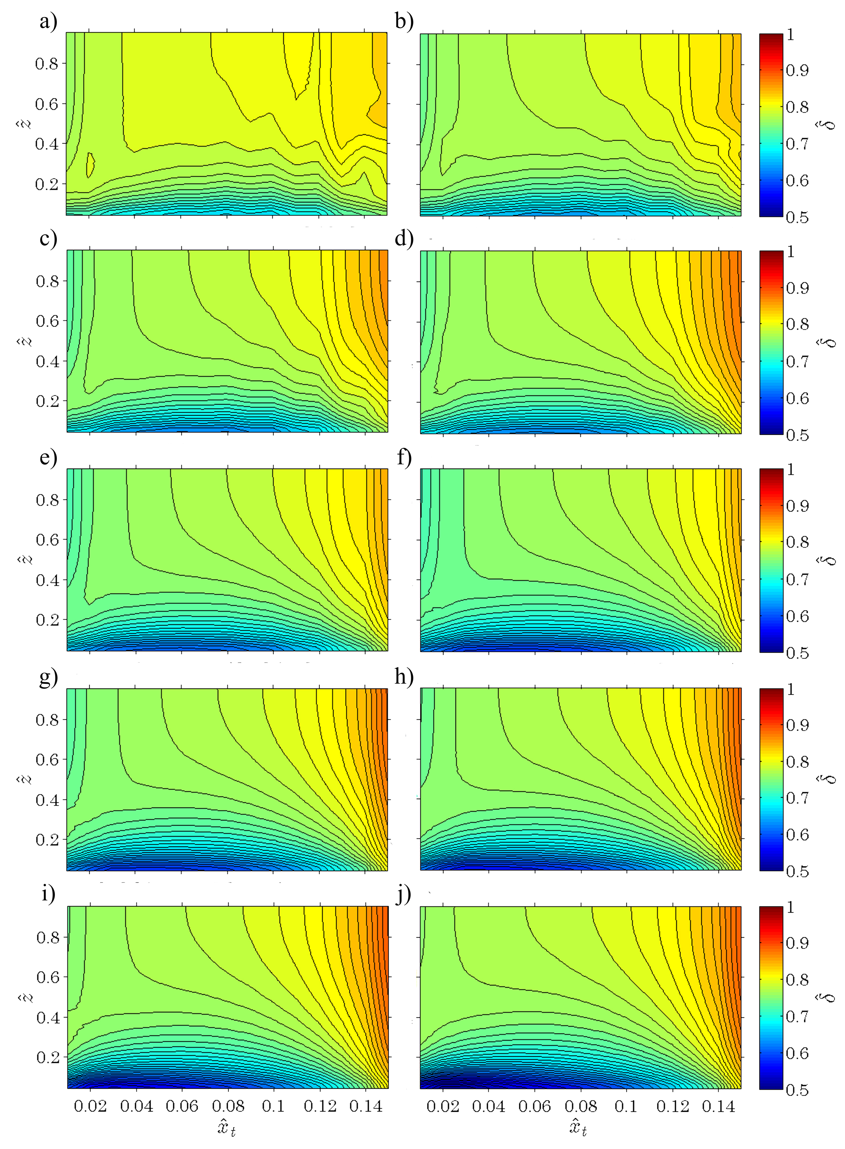
Figure 13 shows, for each layout, the distribution of the -angle at the tributary entrance. It is readily noticeable that, close to the bottom, the flow deflection angles assume lower values than those at the surface (especially near the upstream junction corner), where the resulting vector () tends to maintain the same direction as that of the tributary, but always with . This trend is more visible at high -angles (from Figure 13f–j), where is about 0.5 at the bottom and near the upstream lateral wall, while it is about 0.9 at the surface near the downstream junction corner.
This means that, as increases, the confluent channels undergo a progressively greater deflection with respect to the flow direction in the post-confluence channel, as it was observed also by Best [1]. Furthermore, it confirms that, near the left bank of the tributary channel, the degree of flow retardation increases.
It is also evident that at low -values the penetration of the main channel flow into the tributary channel flow never occurs.
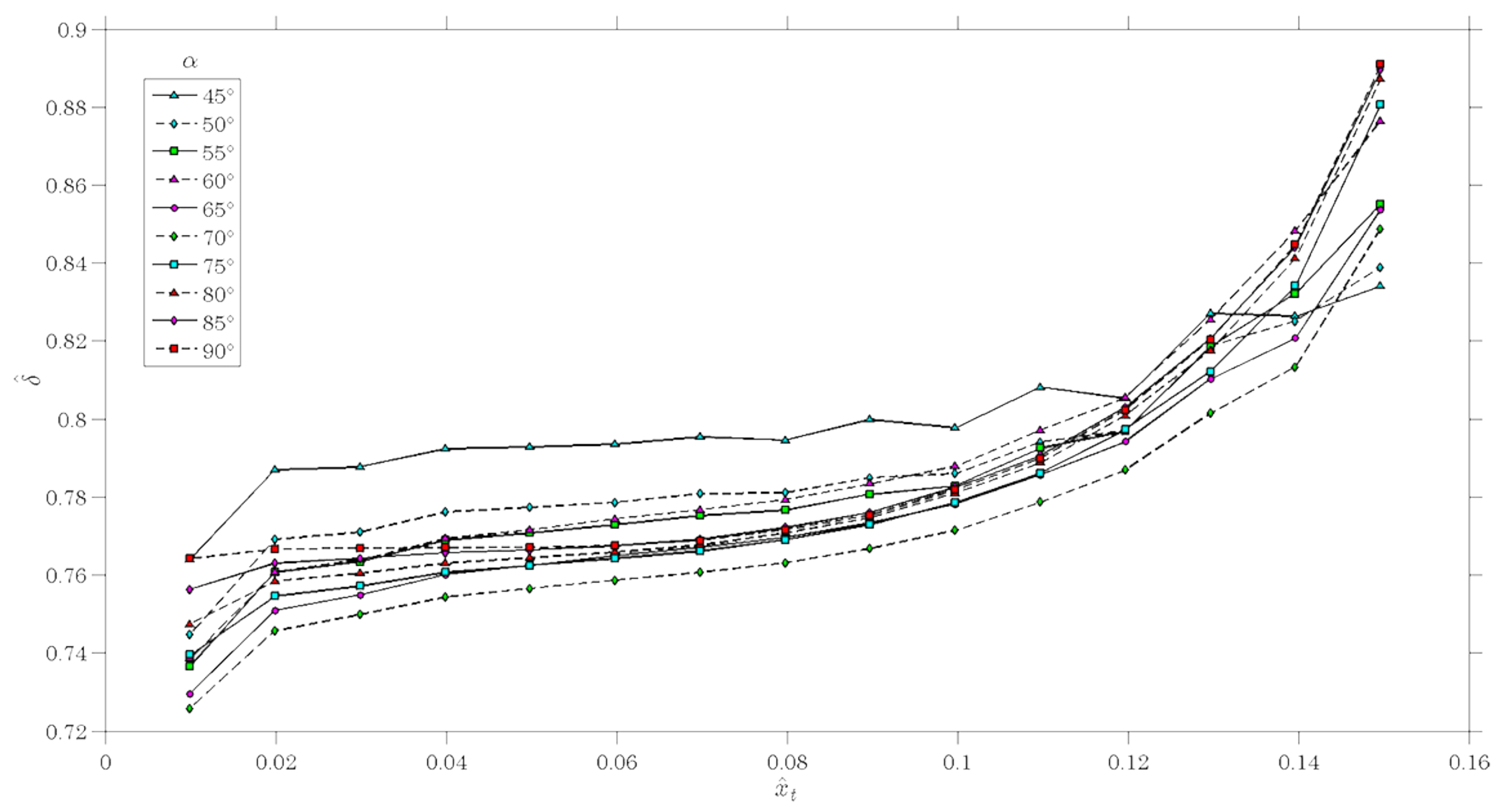
Extrapolating the data at elevation , a direct comparison among the different distributions of the deflection angle along the -axis is shown in Figure 14. It is possible to note that all the data collapse within a band, with a slight deviation for the case of . In particular, increases along the interfacial plane between the tributary and the main channels, assuming the maximum values near the downstream junction corner (as it was observed by Djordjevic [12]), whereas the variability of for is limited in the range 0.76 ÷ 0.83, owing to the combination of low , and , which leads to a more uniform distribution of across the interfacial layer between the tributary and the main channel flows.
3.3. Flow Separation Zone
The analysis on the tributary flow deflection demonstrates that, at the downstream junction corner, is always lower than , which means that, in correspondence of this point, the velocity vectors have a streamwise component that is neither zero nor negative. Such a behaviour supported the procedure proposed in this study for the definition of the separation zone, which is based on the assumption that the separation point is not coincident with the junction point, but it is located downstream of it.
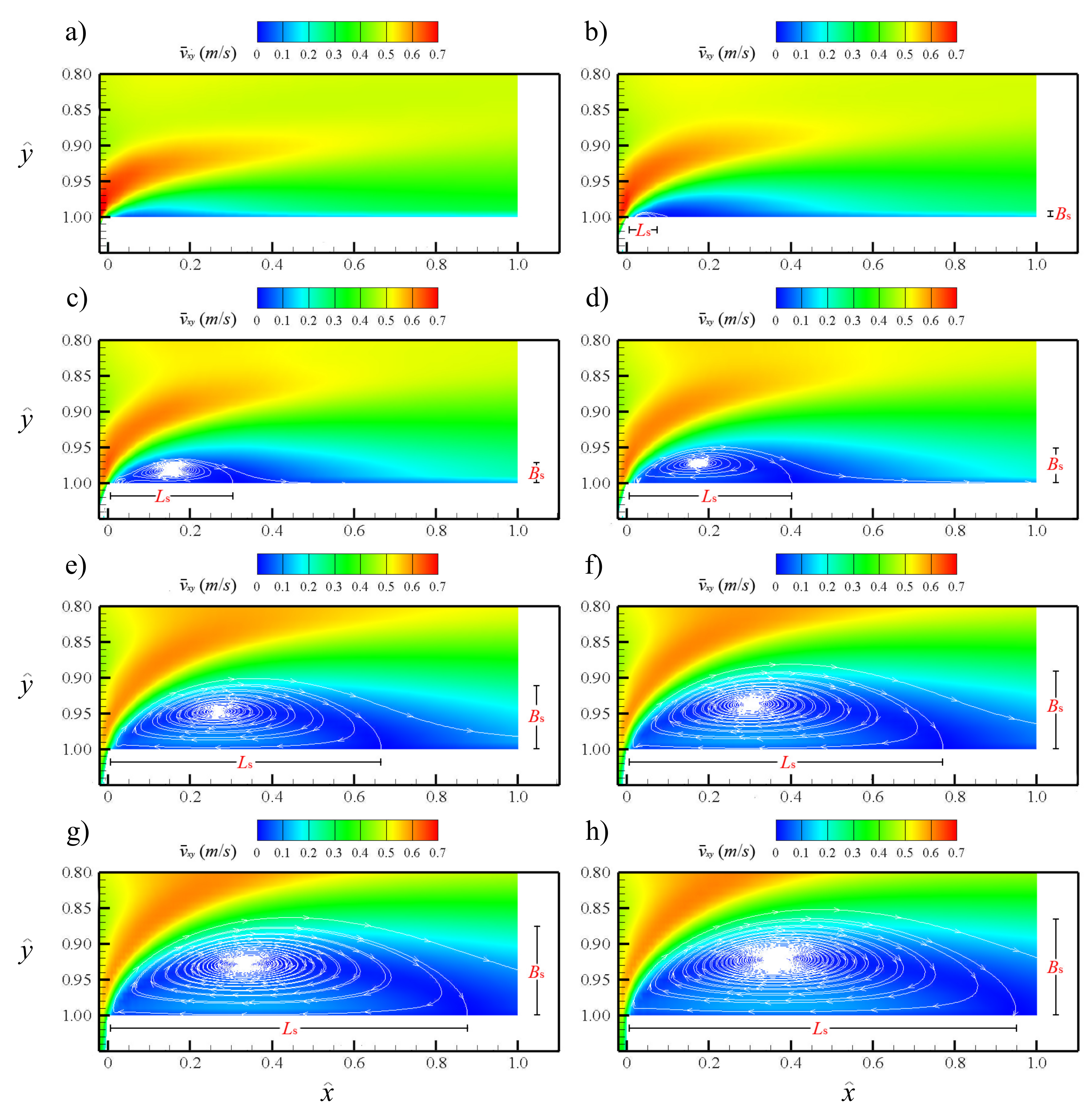
Figure 15 shows the time-averaged velocity in the horizontal plane , obtained by the numerical simulations, and the shape of the flow separation zone for the analysed layouts. It is evident that, as increases, the separation zone becomes longer and wider. This trend is the same of that reported in other studies (see Introduction). For example, Best and Reid [16] found that increasing the junction angle and, also, the contribution of the tributary to total discharge results in an increase of the width and length of the flow-separation zone.
Anyway, this behaviour confirms the findings regarding the flow deflection zone: at the downstream bank of the tributary, the higher the deflection angles (occurring in the case of high junction angles), the stronger the separation downstream of the confluence (as observed by Djordjevic [12]). Furthermore, it is possible to note, especially for low values, that the separation point is always located beyond the origin of the downstream junction angle, as it was specified previously.
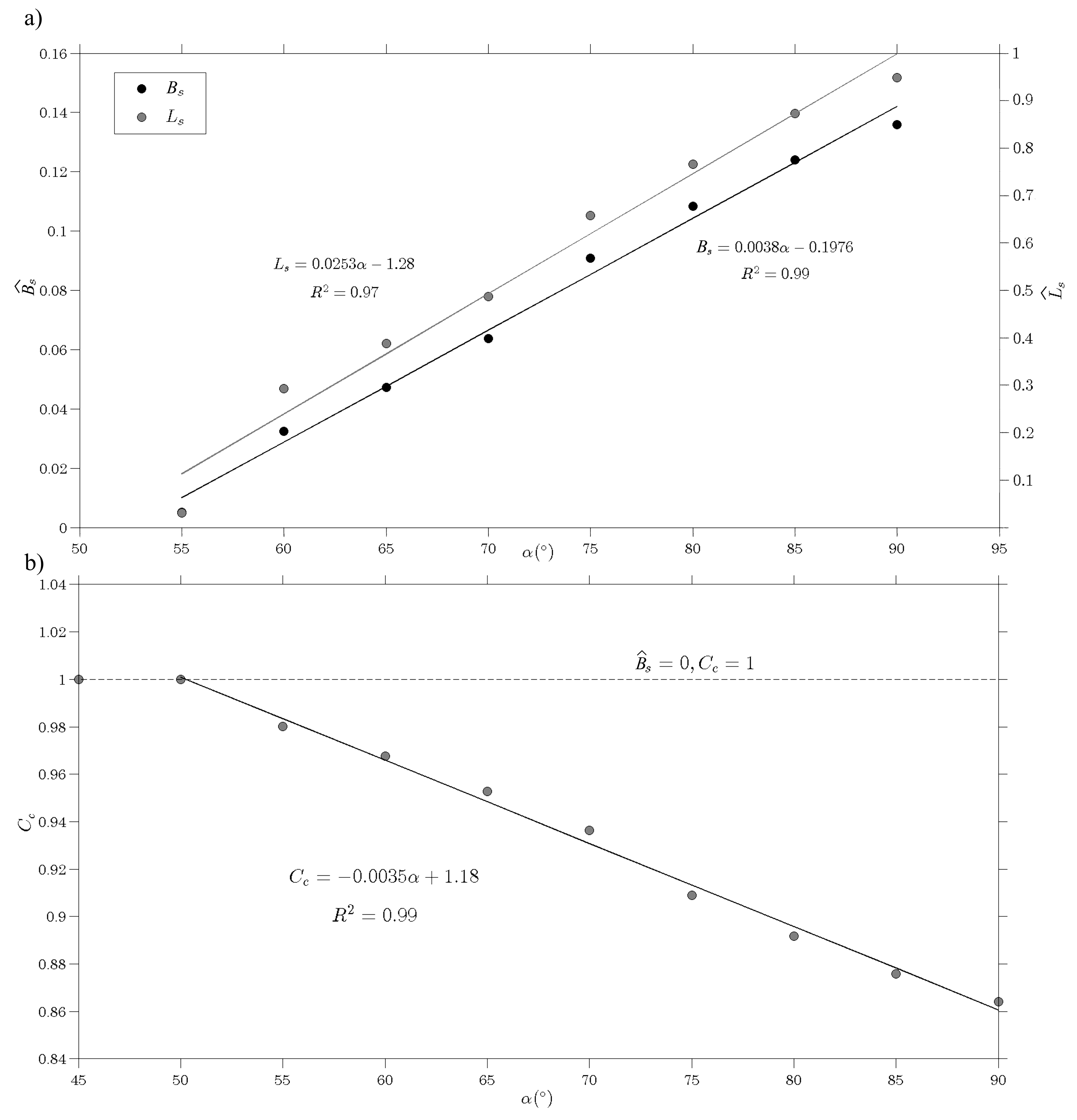
The dimensions and were calculated for each confluence angle and were plotted in Figure 16a after normalisation with (, ). Specifically, they are linearly correlated with according to the equations shown in Figure 16a, with a coefficient of determination () equal to 0.97 for and 0.99 for . It is important to highlight that, in contrast with the literature findings, the separation zone does not occupy the half of the width of the post-confluence channel, as it was observed in other studies with high . In fact, it is confined within about 13 cm from the wall (inner bank of the flume), considering that its maximum width occurs at = . Only Hsu et al. [27], for = 1, obtained a value of comparable with that reported here.
For junction angles less than , the separation zone is no longer observed, owing to the low deflection angles with respect to at the tributary entrance into the confluence. Therefore, it is possible to state that, in the geometrical and hydraulic conditions of the present study, the separation zone starts appearing for between and . However, it is important to point out that this result is valid for the particular case of highly channelized confluences, since it was demonstrated by several authors that the flow separation might be suppressed by the gentle curvature of natural confluence corners (e.g., [5]).
3.4. Contraction Zone and Maximum Streamwise Velocity
The flow separation causes the establishment of a contraction zone beside it, in which the flow is forced to increase its velocity. The reason behind this fact is the reduction of the effective width of the post-confluence channel. To quantify such reduction, a contraction coefficient was calculated as for all the analysed layouts, as shown in Figure 16b. It is illustrated how decreases linearly as increases, since the width of the separation zone increases. The result is coherent with the findings observed in Figure 16a, for the recirculation width . Aiming at giving a relationship that would be useful in 1D modelling to determine the effective mean velocity in the post-confluence channel, an equation is proposed in Figure 16b, valid for low values of and . Obviously, is equal to 1 for less than , since no separation zone occurs ( = 0).
The contraction coefficient can be used for the determination of the head losses () at junctions with the Borda–Carnot formula for a sudden flow expansion (e.g., [15]) as (where is the mean velocity in the post-confluence channel). In turn, can be used to estimate the water level elevations in the separation and contraction zones. Specifically, since decreases as increases, it is expected that the head losses increase as well. This means that a reduced extent of the separation zone will lead to lesser water level differences. Note that the local decrease in water level in correspondence with the separation zone had been noted in many laboratory experiments, including that of Birjukova et al. [23].
Table 2 shows the position in the computational domain and the value of the non-dimensional maximum streamwise velocity (normalised with = 0.049 ms) in the flow field at each analysed layout, being the distance from the downstream junction corner and the distance from the inner bank of the post-confluence channel to the point in which the streamwise velocity achieves its maximum value.
It is readily noticeable that the maximum velocity occurs at = and, then, increasing the junction angle, it starts to decrease up to = , where a reverse trend leads to an increasing of . This tendency could be justified considering the interference induced by the separation zone into the main channel flow and also by the increased discharge due to the added tributary flow. In fact, for = , owing to the low entrance angle of the lateral flow, the tributary flow almost does not interfere with the main channel flow. The separation zone does not exist and, therefore, the zone of maximum flow velocity is confined near the wall ( = 1 cm) at the downstream junction corner ( = 0 cm), occupying a very small area. For = , this area becomes wider and, since the discharge of the tributary flow is not changed, the maximum flow velocity in the post-confluence channel is smaller than for = . Note that, also in this case, since no separation occurs, the maximum flow velocity zone is confined near the wall ( = 2 cm) at the downstream junction corner ( = 0 cm). Increasing , the streamwise velocity component reduces its magnitude because the flow acceleration is limited, owing to the presence of the separation zone that always gets wider. The maximum velocity zone increases its width too. This trend is visible up to = . It should be highlighted that the numerical simulations are in accordance with the experiment of Birjukova et al. [23], since it was demonstrated that the zone of generally high streamwise velocities is located from 4 cm to 40 cm beyond the downstream junction corner for = . Starting from = , the streamwise maximum flow velocity increases and it is found at 35 ÷ 38 cm from the wall and at 43 ÷ 50 cm from the downstream junction corner. This means that such velocity values are not related to the acceleration induced by the lateral flow that approaches the post-confluence channel, which continues to decrease increasing . They are, instead, due to the increased discharge, owing to the tributary flow that should pass through the contraction section.
Therefore, as it was discussed and unlike the common opinion or other literature findings (e.g., [1,29]), in the case of a channel confluence with low and , the maximum velocity does not necessarily occur in the contraction zone, but rather along the inner wall. This clarification is important with respect to possible scouring phenomena that can occur in correspondence of the maximum velocity zone and, thus, of the maximum bed shear stresses, in the case of mobile beds.
4. Conclusions
This paper constitutes a novelty in the study of the dynamics of open-channel confluences, since it focuses on a particular type of confluence characterized by fixed concordant beds and low width and discharge ratios. Specifically, it illustrates the development of the flow structure increasing the junction angle from 45 to 90. The paper is based on numerical simulations performed with the use of the PANORMUS code adapted ad hoc, which were compared and calibrated with the experiment performed by Birjukova et al. [23] for equal to . Ten different junction angles were analysed, focusing on the retardation zone in both the main and tributary channels, the deflection of the tributary flow from the junction angle, the extension of the separation zone downstream the channel confluence and the maximum streamwise velocity. The simulation results and analysis suggested that, as increases:
- near the upstream lateral bank of the tributary channel, the degree of flow retardation increases, which implies wider and longer retardation zone and lower velocity in this region. In fact, the streamwise distance between the upstream junction corner and the point decreases with increasing , as well as the lateral distance between the upstream junction corner and the point ;
- the confluent channels undergo a progressively greater deflection with respect to the flow direction in the post-confluence channel. Specifically, for all the junction angles, the deflection of the flow in the horizontal plane at the tributary entrance to the confluence increases along the interfacial plane between the tributary and the main channels, except for = 45, where its distribution was more uniform than in the other cases, owing to the combination of low , and ;
- the separation zone becomes longer and wider, following a linear relationship, since, at the downstream lateral bank of the tributary, the higher the deflection angles (occurring in the case of high junction angles), the higher the separation downstream of the confluence. Moreover, for less than 55, the separation zone is no longer observed, owing to the low discharge ratio and deflection angles with respect to at the tributary entrance into the confluence;
- the contraction coefficient decreases linearly, since the width of the separation zone increases. The determination of this coefficient would be useful in 1D modelling to determine the effective mean velocity in the post-confluence channel;
- the maximum streamwise flow velocity in the whole confluence region does not necessarily increase because it does not always occur in the contraction zone. This fact could be caused by the acceleration induced by the lateral flow that approaches the post-confluence channel, especially in the case of low , and .
Acknowledgments
This research was supported by the European Commission, the European Social Fund and the Regione Calabria. The authors are the only ones responsible for this research. The European Commission and the Regione Calabria are not responsible for any use that may be made of the information contained therein.
Author Contributions
Olga B. Canelas and António H. Cardoso designed and performed the laboratory test; Nadia Penna and Mauro De Marchis designed the numerical simulations; Mauro De Marchis and Enrico Napoli carried out the numerical simulations; Nadia Penna, Mauro De Marchis and Roberto Gaudio analysed experimental and numerical results. The finalization of the paper draft was made by Nadia Penna.
Conflicts of Interest
The authors declare no conflict of interest.
References
- Best, J.L. Flow dynamics at river channel confluences: Implications for sediment transport and bed morphology. In Recent Developments in Fluvial Sedimentology; Ethridge, F.G., Flores, R.M., Harvey, M.D., Eds.; SEPM Society for Sedimentary Geology: Tulsa, OK, USA, 1987; pp. 27–35. [Google Scholar]
- Taylor, E.H. Flow characteristics at rectangular open-channel junctions. J. Trans. 1944, 109, 893–902. [Google Scholar]
- Biron, P.; Best, J.L.; Roy, A.G. Effects of bed discordance on flow dynamics at open channel confluences. J. Hydraul. Eng. 1996, 122, 676–682. [Google Scholar] [CrossRef]
- Leite Ribeiro, M.; Blanckaert, K.; Roy, A.; Schleiss, A.J. Flow and sediment dynamics in channel confluences. J. Geophys. Res. Earth Surf. 2012, 117. [Google Scholar] [CrossRef]
- Roy, A.G.; Roy, R.; Bergeron, N. Hydraulic geometry and changes in flow velocity at a river confluence with coarse bed material. Earth Surf. Process. Landf. 1988, 13, 583–598. [Google Scholar] [CrossRef]
- Rhoads, B.L.; Sukhodolov, A.N. Field investigation of three-dimensional flow structure at stream confluences: 1. Thermal mixing and time-averaged velocities. Water Resour. Res. 2001, 37, 2393–2410. [Google Scholar] [CrossRef]
- Riley, J.D.; Rhoads, B.L.; Parsons, D.R.; Johnson, K.K. Influence of junction angle on three-dimensional flow structure and bed morphology at confluent meander bends during different hydrological conditions. Earth Surf. Process. Landf. 2015, 40, 252–271. [Google Scholar] [CrossRef]
- Gualtieri, C.; Filizola, N.; de Oliveira, M.; Santos, A.M.; Ianniruberto, M. A field study of the confluence between Negro and Solimões Rivers. Part 1: Hydrodynamics and sediment transport. C. R. Geosci. 2018, 350, 31–42. [Google Scholar] [CrossRef]
- Ianniruberto, M.; Trevethan, M.; Pinheiro, A.; Andrade, J.F.; Dantas, E.; Filizola, N.; Santos, A.; Gualtieri, C. A field study of the confluence between Negro and Solimões Rivers. Part 2: Bed morphology and stratigraphy. C. R. Geosci. 2018, 350, 43–54. [Google Scholar] [CrossRef]
- Biron, P.M.; Ramamurthy, A.S.; Han, S. Three-dimensional numerical modeling of mixing at river confluences. J. Hydraul. Eng. 2004, 130, 243–253. [Google Scholar] [CrossRef]
- Constantinescu, G.; Miyawaki, S.; Rhoads, B.; Sukhodolov, A.; Kirkil, G. Structure of turbulent flow at a river confluence with momentum and velocity ratios close to 1: Insight provided by an eddy-resolving numerical simulation. Water Resour. Res. 2011, 47. [Google Scholar] [CrossRef]
- Djordjevic, D. Numerical study of 3D flow at right-angled confluences with and without upstream planform curvature. J. Hydroinform. 2013, 15, 1073–1088. [Google Scholar]
- Webber, N.B.; Greated, C. An investigation of flow behaviour at the junction of rectangular channels. Proc. Inst. Civ. Eng. 1966, 34, 321–334. [Google Scholar] [CrossRef]
- Ramamurthy, A.S.; Carballada, L.B.; Tran, D.M. Combining open channel flow at right angled junctions. J. Hydraul. Eng. 1988, 114, 1449–1460. [Google Scholar] [CrossRef]
- Schindfessel, L.; Creëlle, S.; De Mulder, T. How Different Cross-Sectional Shapes Influence the Separation Zone of an Open-Channel Confluence. J. Hydraul. Eng. 2017, 143, 04017036. [Google Scholar] [CrossRef]
- Best, J.L.; Reid, I. Separation zone at open-channel junctions. J. Hydraul. Eng. 1984, 110, 1588–1594. [Google Scholar] [CrossRef]
- Gurram, S.K.; Karki, K.S.; Hager, W.H. Subcritical junction flow. J. Hydraul. Eng. 1997, 123, 447–455. [Google Scholar] [CrossRef]
- Shumate, E.D. Experimental Description of Flow at an Open-Channel Junction. Ph.D. Thesis, University of Iowa, Iowa City, IA, USA, 1998. [Google Scholar]
- Wang, X.; Wang, X.; Lu, W.; Liu, T. Experimental study on flow behavior at open channel confluences. Front. Archit. Civ. Eng. China 2007, 1, 211–216. [Google Scholar] [CrossRef]
- Qing-Yuan, Y.; Xian-Ye, W.; Wei-Zhen, L.; Xie-Kang, W. Experimental study on characteristics of separation zone in confluence zones in rivers. J. Hydrol. Eng. 2009, 14, 166–171. [Google Scholar] [CrossRef]
- Biswal, S.; Mohapatra, P.; Muralidhar, K. Flow separation at an open channel confluence. J. Hydraul. Eng. 2010, 16, 89–98. [Google Scholar] [CrossRef]
- Schindfessel, L.; Creëlle, S.; Boelens, T.; De Mulder, T. Flow patterns in an open channel confluence with a small ratio of main channel to tributary discharge. In Proceedings of the 7th International Conference on Fluvial Hydraulics (River Flow), Lausanne, Switzerland, 3–5 September 2014; Taylor & Francis Group: London, UK, 2014; pp. 989–996. [Google Scholar]
- Birjukova, O.; Guillen, S.; Alegria, F.; Cardoso, A.H. Three dimensional flow field at confluent fixed-bed open channels. In Proceedings of the 7th International Conference on Fluvial Hydraulics (River Flow), Lausanne, Switzerland, 3–5 September 2014; Crc Press-Taylor & Francis Group: London, UK, 2014; pp. 1007–1014. [Google Scholar]
- Yuan, S.; Tang, H.; Xiao, Y.; Qiu, X.; Zhang, H.; Yu, D. Turbulent flow structure at a 90-degree open channel confluence: Accounting for the distortion of the shear layer. J. Hydro-Environ. Res. 2016, 12, 130–147. [Google Scholar] [CrossRef]
- Lin, J.; Soong, H. Junction losses in open channel flows. Water Resour. Res. 1979, 15, 414–418. [Google Scholar] [CrossRef]
- Hsu, C.C.; Lee, W.J.; Chang, C.H. Subcritical open-channel junction flow. J. Hydraul. Eng. 1998, 124, 847–855. [Google Scholar] [CrossRef]
- Hsu, C.C.; Wu, F.S.; Lee, W.J. Flow at 90 equal-width open-channel junction. J. Hydraul. Eng. 1998, 124, 186–191. [Google Scholar] [CrossRef]
- Bradbrook, K.; Lane, S.; Richards, K.; Biron, P.; Roy, A. Role of bed discordance at asymmetrical river confluences. J. Hydraul. Eng. 2001, 127, 351–368. [Google Scholar] [CrossRef]
- Shakibainia, A.; Tabatabai, M.R.M.; Zarrati, A.R. Three-dimensional numerical study of flow structure in channel confluences. Can. J. Civ. Eng. 2010, 37, 772–781. [Google Scholar] [CrossRef]
- Bonakdari, H.; Lipeme-Kouyi, G.; Wang, X. Experimental validation of CFD modeling of multiphase flow through open channel confluence. In Proceedings of the World Environmental and Water Resources Congress 2011: Bearing Knowledge for Sustainability, Palm Springs, CA, USA, 22–26 May 2011; pp. 2176–2183. [Google Scholar]
- Yang, Q.; Liu, T.; Lu, W.; Wang, X. Numerical simulation of confluence flow in open channel with dynamic meshes techniques. Adv. Mech. Eng. 2013, 5, 860431. [Google Scholar] [CrossRef]
- Brito, M.; Canelas, O.; Leal, J.; Cardoso, A. 3D numerical simulation of flow at a 70° open-channel confluence. In Proceedings of the V Conferencia Nacional de Mecanica dos Fluidos, Termodinamica e Energia, Porto, Portugal, 11–12 September 2014. [Google Scholar]
- Schindfessel, L.; Creëlle, S.; De Mulder, T. Flow patterns in an open channel confluence with increasingly dominant tributary inflow. Water 2015, 7, 4724–4751. [Google Scholar] [CrossRef] [Green Version]
- Guillén-Ludeña, S.; Franca, M.; Cardoso, A.; Schleiss, A. Evolution of the hydromorphodynamics of mountain river confluences for varying discharge ratios and junction angles. Geomorphology 2016, 255, 1–15. [Google Scholar] [CrossRef]
- Napoli, E. PANORMUS Users Manual; University di Palermo: Palermo, Italy, 2011. [Google Scholar]
- Rodríguez, J.F.; García, M.H. Laboratory measurements of 3-D flow patterns and turbulence in straight open channel with rough bed. J. Hydraul. Res. 2008, 46, 454–465. [Google Scholar] [CrossRef]
- Blanckaert, K.; Duarte, A.; Schleiss, A.J. Influence of shallowness, bank inclination and bank roughness on the variability of flow patterns and boundary shear stress due to secondary currents in straight open-channels. Adv. Water Resour. 2010, 33, 1062–1074. [Google Scholar] [CrossRef]
- Defina, A. Transverse spacing of low-speed streaks in a channel flow over a rough bed. Coherent Flow Struct. Open Channels 1996, 4, 87–99. [Google Scholar]
- Barros, J.M.; Christensen, K.T. Observations of turbulent secondary flows in a rough-wall boundary layer. J. Fluid Mech. 2014, 748. [Google Scholar] [CrossRef]
- Willingham, D.; Anderson, W.; Christensen, K.T.; Barros, J.M. Turbulent boundary layer flow over transverse aerodynamic roughness transitions: Induced mixing and flow characterization. Phys. Fluids 2014, 26, 025111. [Google Scholar] [CrossRef]
- De Marchis, M.; Napoli, E. The effect of geometrical parameters on the discharge capacity of meandering compound channels. Adv. Water Resour. 2008, 31, 1662–1673. [Google Scholar] [CrossRef]
- Chen, X.; Zhu, D.Z.; Steffler, P.M. Secondary currents induced mixing at channel confluences. Can. J. Civ. Eng. 2017, 44, 1071–1083. [Google Scholar] [CrossRef]
Figure 1.
Conceptual model of flow dynamics at river confluences, modified from Best [1]. is the post-confluence discharge; is the junction angle.
Figure 1.
Conceptual model of flow dynamics at river confluences, modified from Best [1]. is the post-confluence discharge; is the junction angle.

Figure 2.
(a) plan view and (b) photograph of the experimental facility used by Birjukova et al. [23] with the measurement grid. Streamwise coordinates of the measured cross-sections: = 0 m, = 0.7 m, = 0.78 m, = 0.95 m, = 1.05 m, = 1.15 m, = 1.25 m, = 1.45 m.
Figure 2.
(a) plan view and (b) photograph of the experimental facility used by Birjukova et al. [23] with the measurement grid. Streamwise coordinates of the measured cross-sections: = 0 m, = 0.7 m, = 0.78 m, = 0.95 m, = 1.05 m, = 1.15 m, = 1.25 m, = 1.45 m.

Figure 3.
Patterns of some hydrodynamic variables at cross-section no. 1: (a) schematic of secondary currents; (b) normalized streamwise velocity component, = /; (c) normalized spanwise velocity component, = /; (d) normalized vertical velocity component, = /.
Figure 3.
Patterns of some hydrodynamic variables at cross-section no. 1: (a) schematic of secondary currents; (b) normalized streamwise velocity component, = /; (c) normalized spanwise velocity component, = /; (d) normalized vertical velocity component, = /.

Figure 4.
Patterns of some hydrodynamic variables at cross-section no. 2: (a) schematic of secondary currents; (b) normalized streamwise velocity component, = /; (c) normalized spanwise velocity component, = /; (d) normalized vertical velocity component, = /.
Figure 4.
Patterns of some hydrodynamic variables at cross-section no. 2: (a) schematic of secondary currents; (b) normalized streamwise velocity component, = /; (c) normalized spanwise velocity component, = /; (d) normalized vertical velocity component, = /.

Figure 5.
Patterns of some hydrodynamic variables at cross-section no. 7: (a) schematic of secondary currents; (b) normalized streamwise velocity component, = /; (c) normalized spanwise velocity component, = /; (d) normalized vertical velocity component, = /.
Figure 5.
Patterns of some hydrodynamic variables at cross-section no. 7: (a) schematic of secondary currents; (b) normalized streamwise velocity component, = /; (c) normalized spanwise velocity component, = /; (d) normalized vertical velocity component, = /.

Figure 6.
Computational domain of the confluence.

Figure 7.
(a) comparison of measured (blue dots) and simulated (green lines) non-dimensional streamwise velocity component profiles in cross-section no. 1; (b) comparison of measured and simulated streamwise velocity components; (c) Root Mean Square Error (RMSE) of the streamwise velocity component profiles from = 0.35 to = 0.75 in cross-section no. 1.

Figure 8.
(a) comparison of measured (blue dots) and simulated (green lines) non-dimensional streamwise velocity component profiles in cross-section no. 3; (b) comparison of measured and simulated streamwise velocity components; (c) RMSE of the streamwise velocity component profiles from = 0.35 to = 0.75 in cross-section no. 3.

Figure 9.
(a) comparison of measured (blue dots) and simulated (green lines) non-dimensional streamwise velocity component profiles in cross-sections Nos. 1, 2 and 3 along four longitudinal profiles; (b) comparison of measured and simulated streamwise velocity components.
Figure 9.
(a) comparison of measured (blue dots) and simulated (green lines) non-dimensional streamwise velocity component profiles in cross-sections Nos. 1, 2 and 3 along four longitudinal profiles; (b) comparison of measured and simulated streamwise velocity components.

Figure 10.
Comparison of measured (blue dots) and simulated (green lines) non-dimensional streamwise velocity component profiles in cross-sections Nos. 1, 3, 7 and 8 along the longitudinal profile .
Figure 10.
Comparison of measured (blue dots) and simulated (green lines) non-dimensional streamwise velocity component profiles in cross-sections Nos. 1, 3, 7 and 8 along the longitudinal profile .

Figure 11.
Time-averaged velocity in the horizontal plane for equal to . Here, = x/ is the non-dimensional abscissa directed in the streamwise direction centred in the downstream corner of the confluence.
Figure 11.
Time-averaged velocity in the horizontal plane for equal to . Here, = x/ is the non-dimensional abscissa directed in the streamwise direction centred in the downstream corner of the confluence.

Figure 12.
Distributions of (a) and (b) with respect to at and of the relative flow velocity at points (c) A and (d) B within the retardation zone with respect to at .
Figure 12.
Distributions of (a) and (b) with respect to at and of the relative flow velocity at points (c) A and (d) B within the retardation zone with respect to at .

Figure 13.
Distribution of the -angle at the tributary entrance for equal to (a) , (b) , (c) , (d) , (e) , (f) , (g) , (h) , (i) , (j) . Here, = / is the non-dimensional abscissa directed in the streamwise direction centred in the upstream corner of the confluence.
Figure 13.
Distribution of the -angle at the tributary entrance for equal to (a) , (b) , (c) , (d) , (e) , (f) , (g) , (h) , (i) , (j) . Here, = / is the non-dimensional abscissa directed in the streamwise direction centred in the upstream corner of the confluence.

Figure 14.
Effects of on the -angle distributions at the tributary entrance into the confluence at .
Figure 14.
Effects of on the -angle distributions at the tributary entrance into the confluence at .

Figure 15.
Time-averaged velocity in the horizontal plane for equal to: (a) ; (b) ; (c) ; (d) ; (e) ; (f) ; (g) ; (h) . Here, = x/ is the non-dimensional abscissa directed in the streamwise direction centred in the downstream corner of the confluence.
Figure 15.
Time-averaged velocity in the horizontal plane for equal to: (a) ; (b) ; (c) ; (d) ; (e) ; (f) ; (g) ; (h) . Here, = x/ is the non-dimensional abscissa directed in the streamwise direction centred in the downstream corner of the confluence.

Figure 16.
(a) non-dimensional width and length of the separation zone as a function of ; (b) distribution of the contraction coefficient as a function of at .
Figure 16.
(a) non-dimensional width and length of the separation zone as a function of ; (b) distribution of the contraction coefficient as a function of at .


Table 1.
Experimental tests and numerical studies on channel confluences in chronological order.
| Reference | Study | Reference of the Experimental Test | |||
|---|---|---|---|---|---|
| Webber and Greated [13] | E | - | 0.25 ÷ 4.00 | 1.00 | 30,60,90 |
| Lin and Soong [25] | E | - | 0.18 ÷ 1.40 | 1.00 | 90 |
| Best and Reid [16] | E | - | 0.11 ÷ 9.00 | 1.00 | 15,45,70,90 |
| Ramamurthy et al. [14] | E | - | 0.30 ÷ 1.50 | 0.99 | 90 |
| Biron et al. [3] | E | - | 1.23 | 0.67 | 30 |
| Gurram et al. [17] | E | - | 0.33 ÷ 3.00 | 0.60 ÷ 1.00 | 30,60,90 |
| Hsu et al. [26] | E | - | 0.11 ÷ 8.90 | 1.00 | 90 |
| Hsu et al. [27] | E | - | 0.09 ÷ 9.31 | 1.00 | 30,45,60 |
| Shumate [18] | E | - | 0.09 ÷ 11.00 | 1.00 | 90 |
| Bradbrook et al. [28] | N | Biron et al. [3] | - | 1.00 | 30,45,60 |
| Biron et al. [10] | N | Biron et al. [3] | 0.67,1.74 | 1.00 | 30,60,90 |
| Wang et al. [19] | E | - | 0.77 | 0.40 | 30 |
| Qing-Yuan et al. [20] | E | - | 0.36 | 0.50 | 90 |
| Biswa et al. [21] | E | - | 0.48 ÷ 2.09 | 1.00 | 90 |
| Shakibainia et al. [29] | N | Shumate [18] | 0.33,1.00,3.00 | 0.66,1.00 | 15,45,90,105 |
| Bonakdari et al. [30] | N | Wang et al. [19] | 0.77 | 0.40 | 30 |
| Djordjevic [12] | N | Shumate [18] | 0.71 | 1.00 | 90 |
| Yang et al. [31] | N | Shumate [18] | 3.00 | 1.00 | 90 |
| Schindfessel et al. [22] | E | - | 3.00,19.00 | 1.00 | 90 |
| Birjukova et al. [23] | E | - | 0.11 | 0.15 | 70 |
| Brito et al. [32] | N | Birjukova et al. [23] | 0.11 | 0.15 | 70 |
| Schindfessel et al. [33] | N | Schindfessel et al. [22] | 0,3.00,19.00 | 1.00 | 90 |
| Yuan et al. [24] | E | - | 0.65 | 1.00 | 90 |
| Schindfessel et al. [15] | N | Schindfessel et al. [22] | 3 | 1.00 | 90 |
E: experimental study; N: numerical study.
Table 2.
Non-dimensional maximum streamwise velocity component at different junction angles.
| (m) | (m) | / | |
|---|---|---|---|
| 45 | 0.00 | 0.010 | 1.475 |
| 50 | 0.00 | 0.020 | 1.336 |
| 55 | 0.10 | 0.070 | 1.238 |
| 60 | 0.15 | 0.100 | 1.231 |
| 65 | 0.16 | 0.110 | 1.211 |
| 70 | 0.20 | 0.130 | 1.205 |
| 75 | 0.43 | 0.355 | 1.224 |
| 80 | 0.45 | 0.355 | 1.249 |
| 85 | 0.49 | 0.380 | 1.272 |
| 90 | 0.50 | 0.380 | 1.290 |
© 2018 by the authors. Licensee MDPI, Basel, Switzerland. This article is an open access article distributed under the terms and conditions of the Creative Commons Attribution (CC BY) license (http://creativecommons.org/licenses/by/4.0/).
Share and Cite
MDPI and ACS Style
Penna, N.; De Marchis, M.; Canelas, O.B.; Napoli, E.; Cardoso, A.H.; Gaudio, R. Effect of the Junction Angle on Turbulent Flow at a Hydraulic Confluence. Water 2018, 10, 469. https://doi.org/10.3390/w10040469
AMA Style
Penna N, De Marchis M, Canelas OB, Napoli E, Cardoso AH, Gaudio R. Effect of the Junction Angle on Turbulent Flow at a Hydraulic Confluence. Water. 2018; 10(4):469. https://doi.org/10.3390/w10040469
Chicago/Turabian StylePenna, Nadia, Mauro De Marchis, Olga B. Canelas, Enrico Napoli, António H. Cardoso, and Roberto Gaudio. 2018. "Effect of the Junction Angle on Turbulent Flow at a Hydraulic Confluence" Water 10, no. 4: 469. https://doi.org/10.3390/w10040469
Note that from the first issue of 2016, this journal uses article numbers instead of page numbers. See further details here.