Glacial Lake Detection from GaoFen-2 Multispectral Imagery Using an Integrated Nonlocal Active Contour Approach: A Case Study of the Altai Mountains, Northern Xinjiang Province


Abstract
:1. Introduction
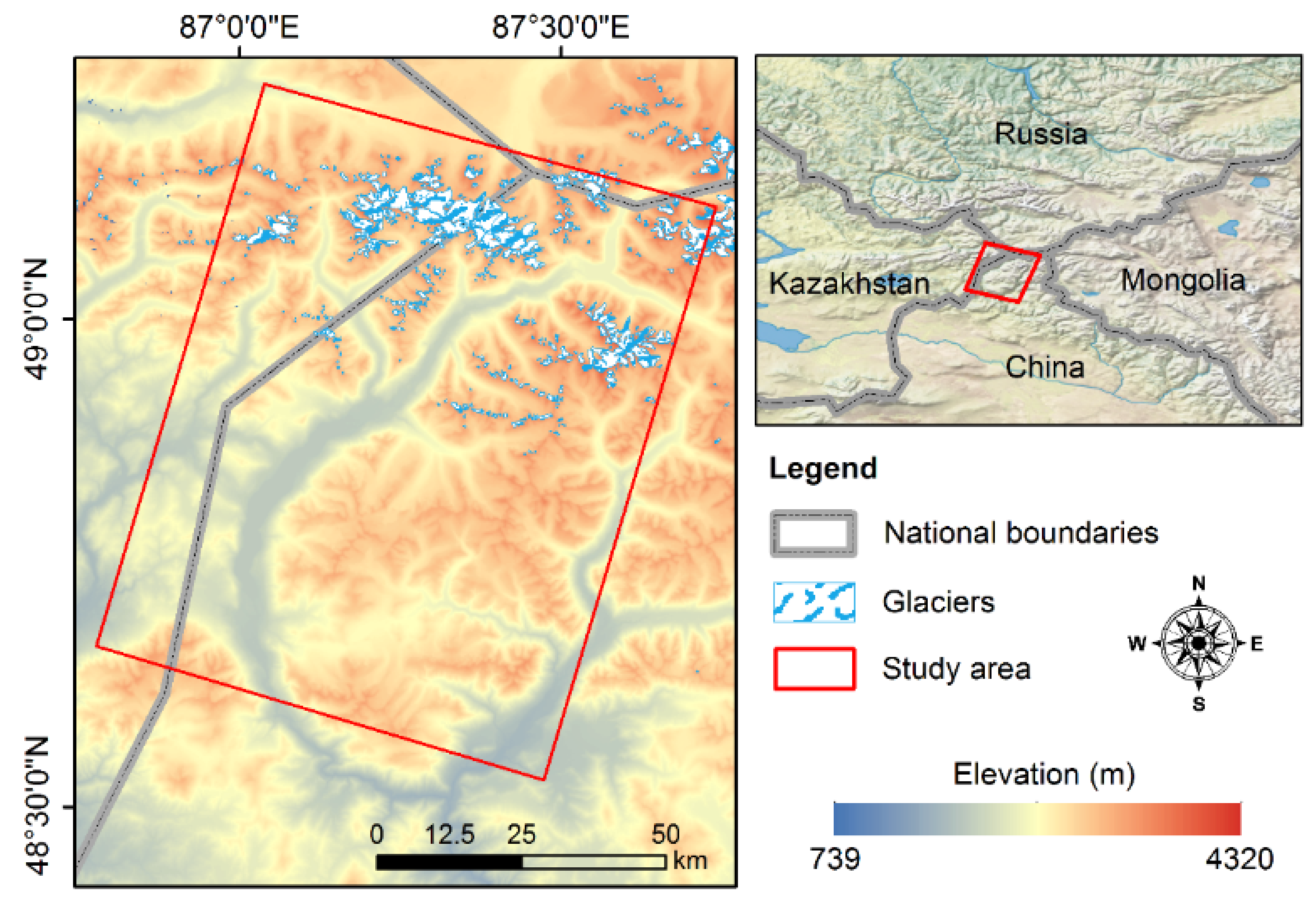
2. Study Area
3. Methodology
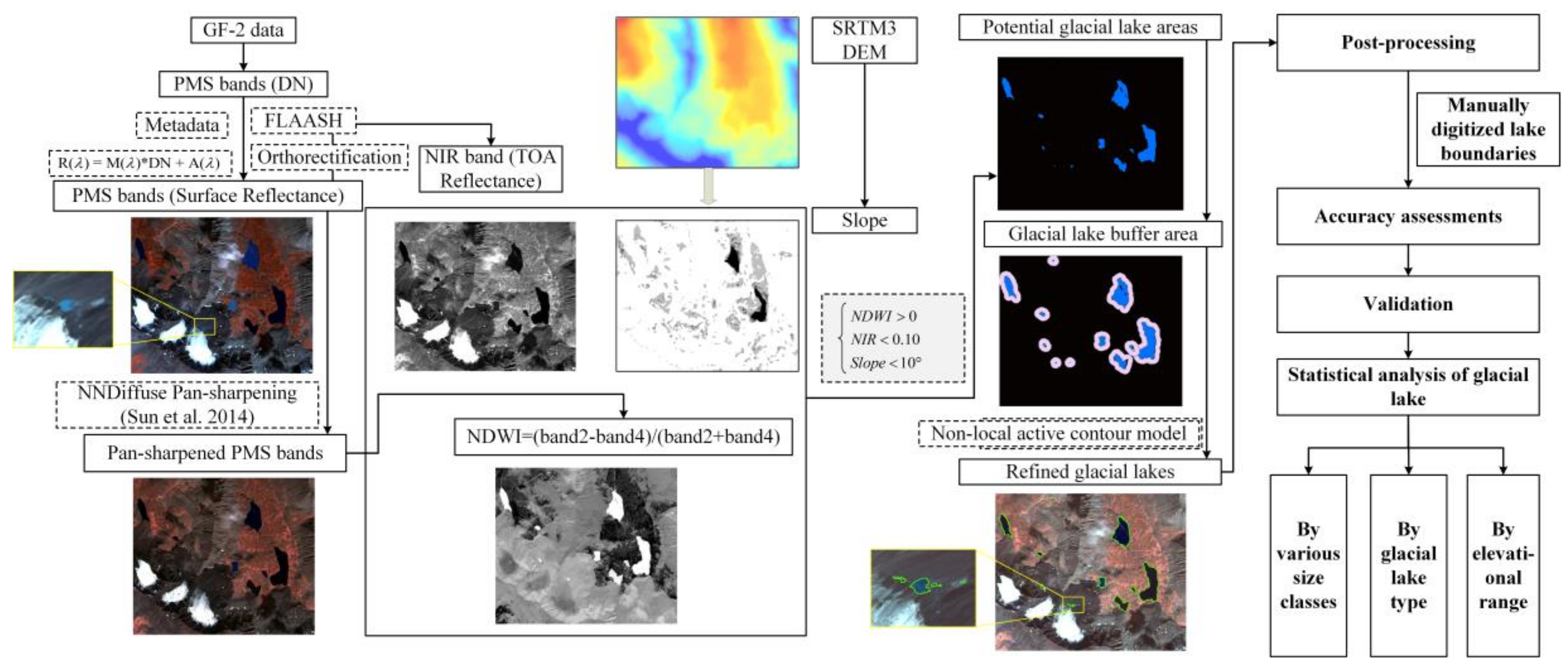
3.1. Data and Workflow of the Proposed Method
3.2. Conversion of PMS Digital Number (DN) to Surface Reflectance (SR)
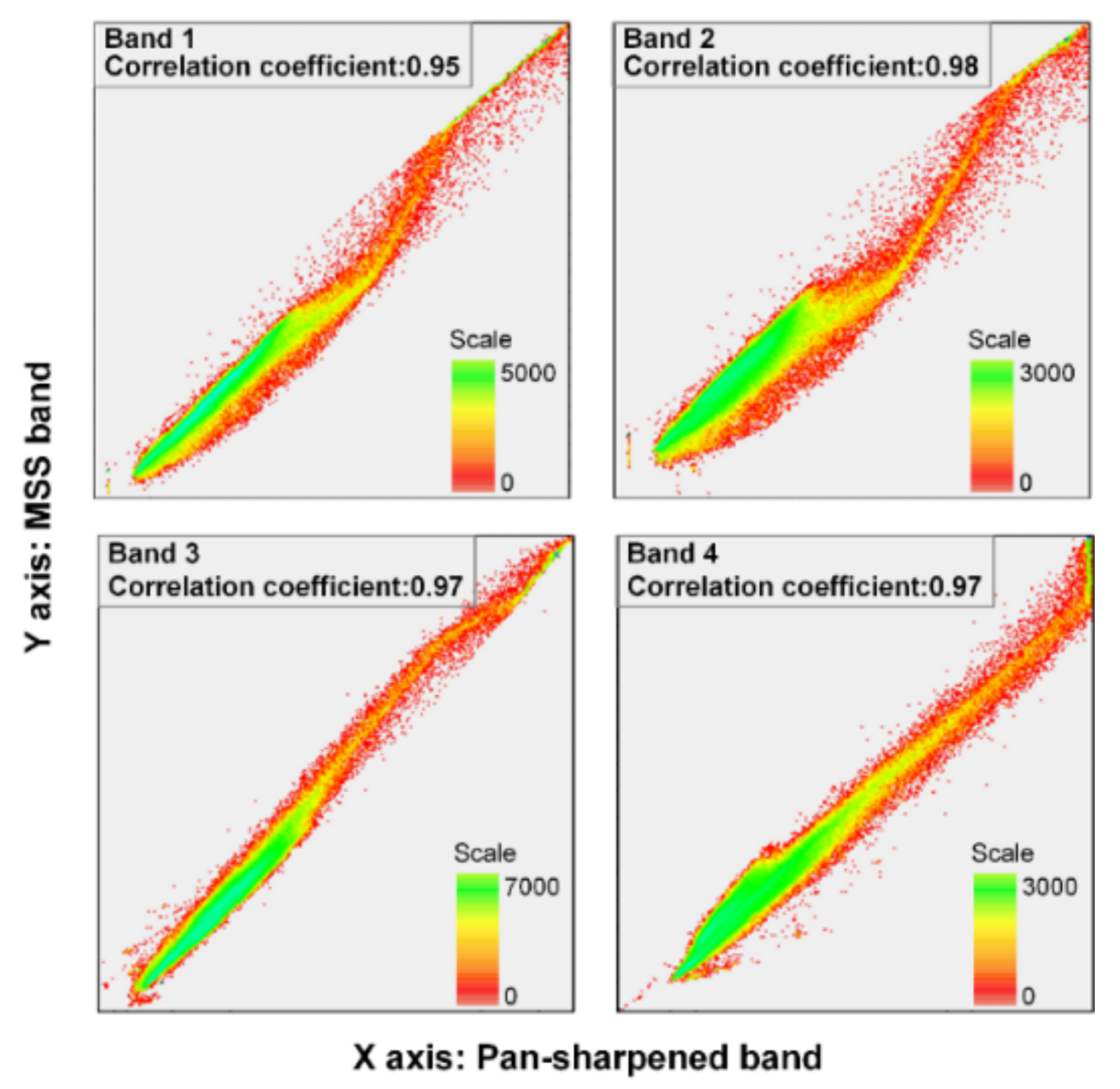
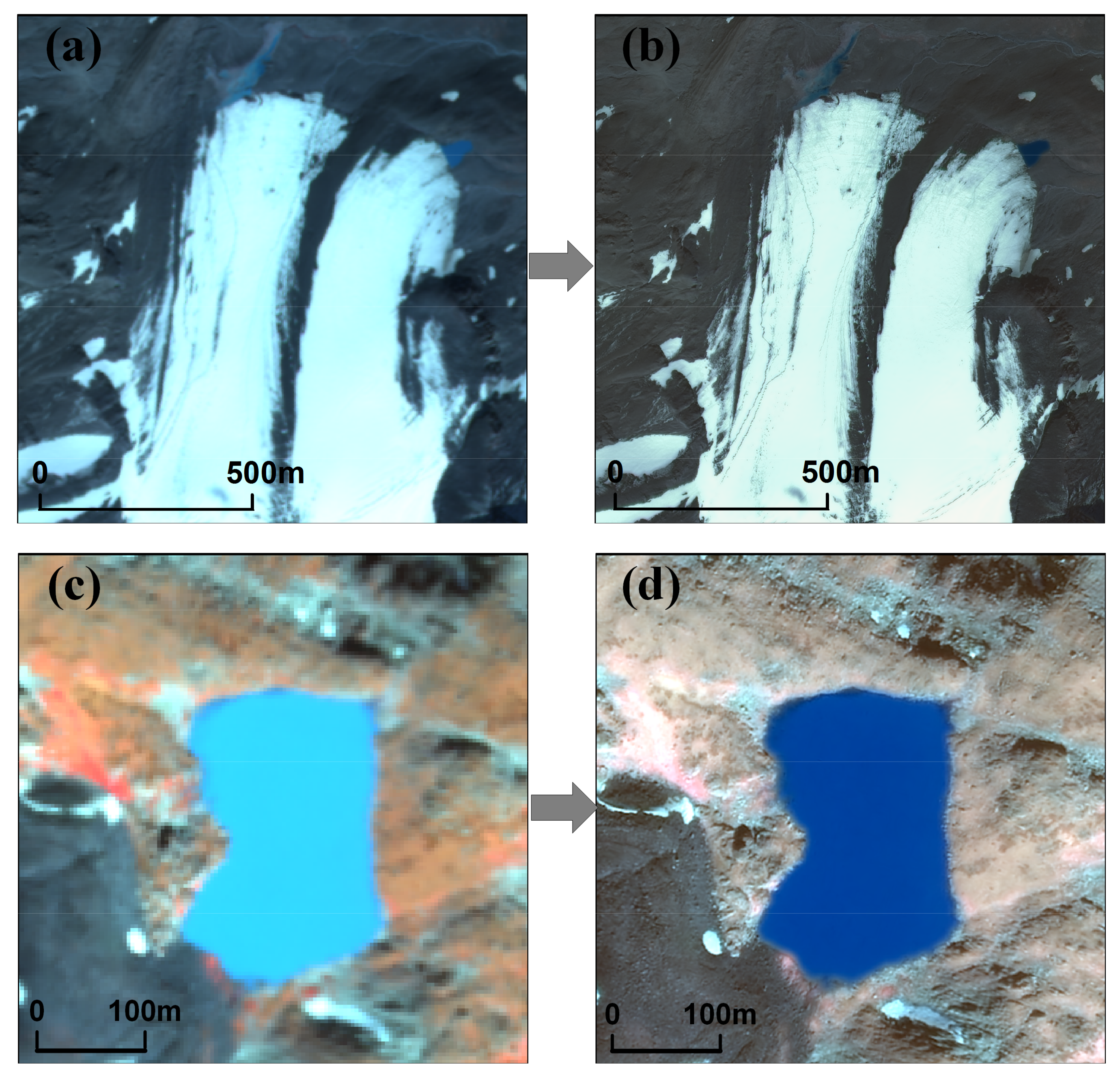
3.3. Pan-Sharpening of PMS Bands
3.4. Generation of Potential Glacial Lakes
3.5. Glacial Lake Detection Algorithm
3.6. Performance Evaluation
4. Results and Discussion
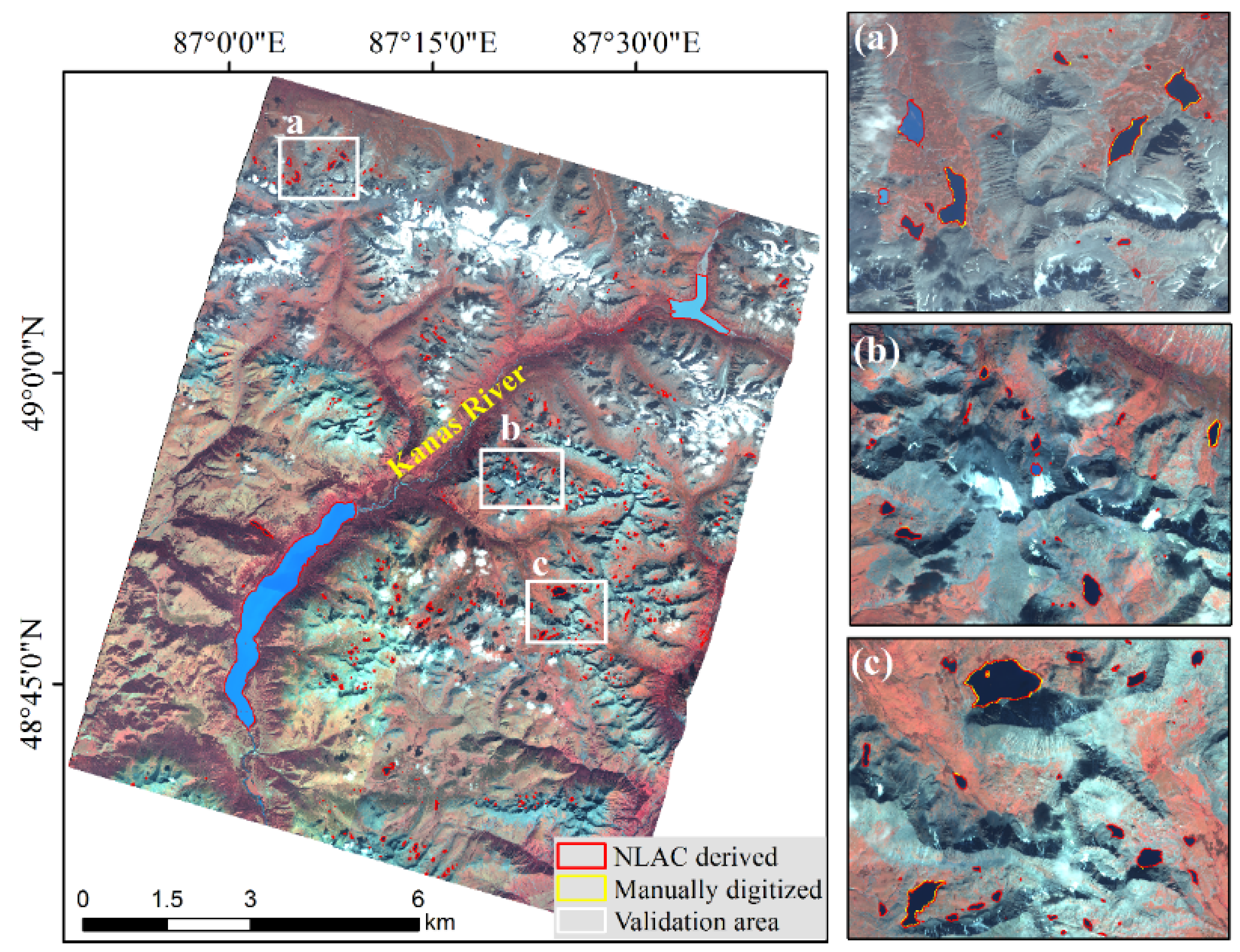
4.1. Mapping of All the Glacial Lakes in the Study Area
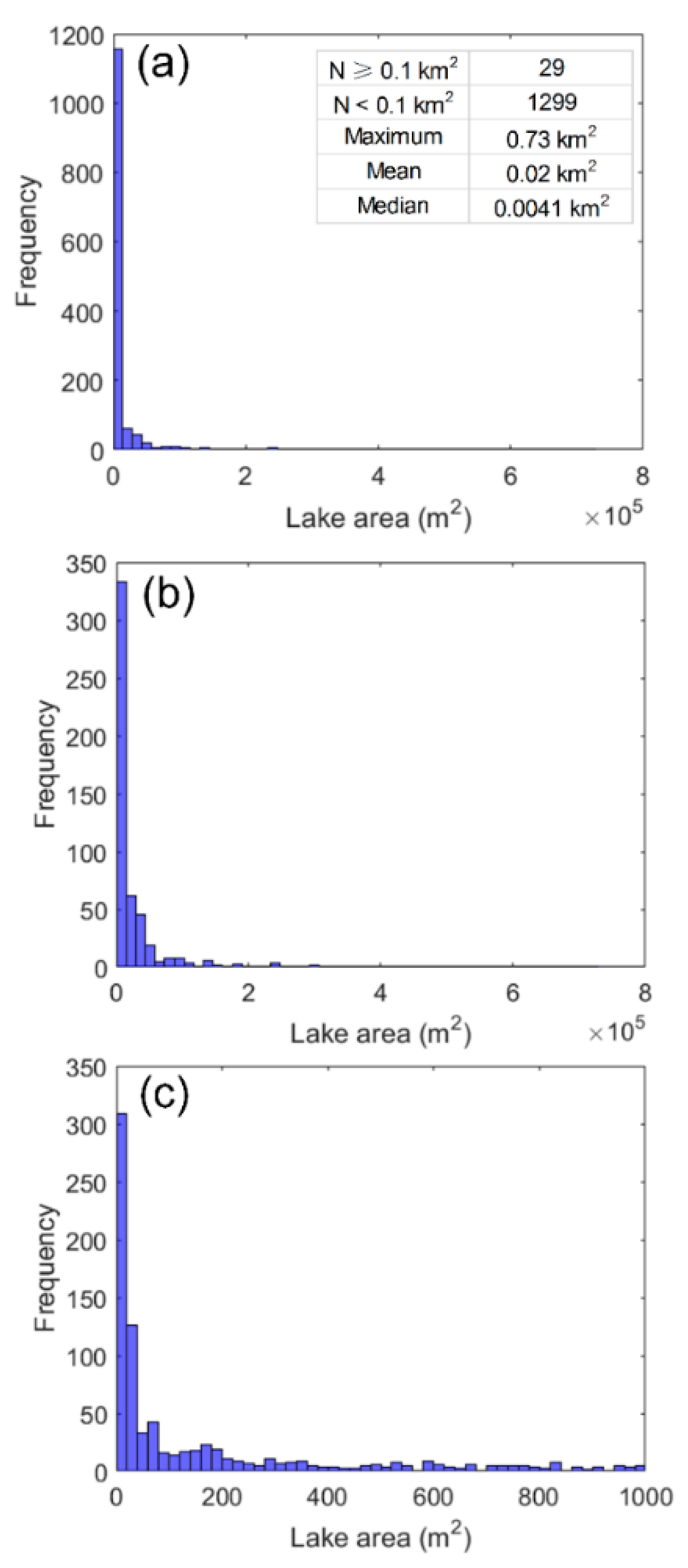
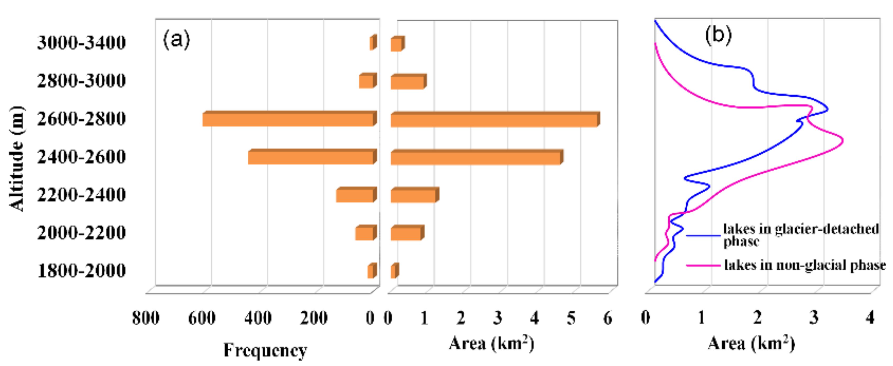
4.2. Distribution Characteristics of Glacial Lakes in Altai Mountains
4.3. Discussion
5. Conclusions
Acknowledgments
Author Contributions
Conflicts of Interest
References
- Prakash, C.; Nagarajan, R. Glacial Lake Inventory and Evolution in Northwestern Indian Himalaya. IEEE J. Sel. Top. Appl. Earth Obs. Remote Sens. 2017, 10, 5284–5294. [Google Scholar] [CrossRef]
- Chen, F.; Zhang, M.M.; Tian, B.S.; Li, Z. Extraction of Glacial Lake Outlines in Tibet Plateau Using Landsat 8 Imagery and Google Earth Engine. IEEE J. Sel. Top. Appl. Earth Obs. Remote Sens. 2017, 10, 4002–4009. [Google Scholar] [CrossRef]
- Moussavi, M.S.; Abdalati, W.; Pope, A.; Scambos, T.; Tedesco, M. Derivation and validation of supraglacial lake volumes on the Greenland Ice Sheet from high-resolution satellite imagery. Remote Sens. Environ. 2016, 183, 294–303. [Google Scholar] [CrossRef]
- Bajracharya, R.S.; Mool, P. Glaciers, glacial lakes and glacial lake outburst floods in the Mount Everest region, Nepal. Ann. Glaciol. 2014, 50, 81–86. [Google Scholar] [CrossRef]
- Westoby, M.J.; Glasser, N.F.; Brasington, J.; Hambrey, M.J.; Quincey, D.J. Modelling outburst floods from moraine-dammed glacial lakes. Earth-Sci. Rev. 2014, 134, 137–159. [Google Scholar] [CrossRef]
- Thompson, S.S.; Benn, D.I.; Dennis, K.; Luckman, A. A rapidly growing moraine-dammed glacial lake on Ngozumpa Glacier, Nepal. Geomorphology 2012, 145, 1–11. [Google Scholar] [CrossRef]
- Wang, W.; Xiang, Y.; Gao, Y.; Lu, A.; Yao, T. Rapid expansion of glacial lakes caused by climate and glacier retreat in the Central Himalayas. Hydrol. Processes 2015, 29, 859–874. [Google Scholar] [CrossRef]
- Zhang, G.; Yao, T.; Xie, H.; Wang, W.; Yang, W. An inventory of glacial lakes in the Third Pole region and their changes in response to global warming. Glob. Planet. Chang. 2015, 131, 148–157. [Google Scholar] [CrossRef]
- Tian, B.S.; Li, Z.; Zhang, M.M.; Huang, L.; Qiu, Y.B. Mapping Thermokarst Lakes on the Qinghai–Tibet Plateau Using Nonlocal Active Contours in Chinese GaoFen-2 Multispectral Imagery. IEEE J. Sel. Top. Appl. Earth Obs. Remote Sens. 2017, 10, 1687–1700. [Google Scholar] [CrossRef]
- Bhardwaj, A.; Singh, M.K.; Joshi, P.K.; Snehmani; Singh, S. A lake detection algorithm (LDA) using Landsat 8 data: A comparative approach in glacial environment. Int. J. Appl. Earth Obs. Geoinf. 2015, 38, 150–163. [Google Scholar] [CrossRef]
- Mergili, M.; Müller, J.P.; Schneider, J.F. Spatio-temporal development of high-mountain lakes in the headwaters of the Amu Darya River (Central Asia). Glob. Planet. Chang. 2013, 107, 13–24. [Google Scholar] [CrossRef]
- Ovakoglou, G.; Alexandridis, T.K.; Crisman, T.L.; Skoulikaris, C.; Vergoset, G.S. Use of MODIS satellite images for detailed lake morphometry: Application to basins with large water level fluctuations. Int. J. Appl. Earth Obs. Geoinf. 2016, 51, 37–46. [Google Scholar] [CrossRef]
- Wessels, R.L.; Kargel, J.S.; Kieffer, H.H. ASTER measurement of supraglacial lakes in the Mount Everest region of the Himalaya. Ann. Glaciol. 2002, 34, 399–408. [Google Scholar] [CrossRef]
- Quincey, D.J.; Richardson, S.D.; Luckman, A.; Lucas, R.M.; Reynolds, J.M. Early recognition of glacial lake hazards in the Himalaya using remote sensing datasets. Glob. Planet. Chang. 2007, 56, 137–152. [Google Scholar] [CrossRef]
- Sheng, Y.; Song, C.; Wang, J.; Lyons, E.A.; Knox, B.R. Representative lake water extent mapping at continental scales using multi-temporal Landsat-8 imagery. Remote Sens. Environ. 2016, 185, 129–141. [Google Scholar] [CrossRef]
- Wang, X.; Siegert, F.; Zhou, A.G.; Frankeet, J. Glacier and glacial lake changes and their relationship in the context of climate change, Central Tibetan Plateau 1972–2010. Glob. Planet. Chang. 2013, 111, 246–257. [Google Scholar] [CrossRef]
- Cheng, Y.; Jin, S.; Wang, M.; Zhu, Y.; Dong, Z. Image Mosaicking Approach for a Double-Camera System in the GaoFen2 Optical Remote Sensing Satellite Based on the Big Virtual Camera. Sensors 2017, 17, 1411. [Google Scholar]
- Bolch, T.; Buchroithner, M.F.; Peters, J.; Baessler, M.; Bajracharya, S. Identification of glacier motion and potentially dangerous glacial lakes in the Mt. Everest region/Nepal using spaceborne imagery. Nat. Hazards Earth Syst. Sci. 2008, 8, 1329–1340. [Google Scholar] [CrossRef]
- Haeberli, W.; Kääb, A.; Mühll, D.V.; Teysseire, P. Prevention of debris flows from outbursts of periglacial lakes at Gruben, Valais, Swiss Alps. J. Glaciol. 2000, 47, 111–122. [Google Scholar] [CrossRef] [Green Version]
- Huggel, C.; Kääb, A.; Haeberli, W.; Teysseire, P.; Paulet, F. Remote sensing based assessment of hazards from glacier lake outbursts: A case study in the Swiss Alps. Can. Geotech. J. 2002, 39, 316–330. [Google Scholar] [CrossRef]
- Frazier, P.S.; Page, K.J. Water body detection and delineation with Landsat TM data. Photogramm. Eng. Remote Sens. 2000, 66, 1461–1467. [Google Scholar]
- McFeeters, S.K. The use of the Normalized Difference Water Index (NDWI) in the delineation of open water features. Int. J. Remote Sens. 1996, 17, 1425–1432. [Google Scholar] [CrossRef]
- Xu, H. Modification of normalised difference water index (NDWI) to enhance open water features in remotely sensed imagery. Int. J. Remote Sens. 2006, 27, 3025–3033. [Google Scholar] [CrossRef]
- Jin, D.U. Study on Water Bodies Extraction and Classification from SPOT Image. J. Remote Sens. 2001, 5, 219–225. [Google Scholar]
- Pekel, J.F.; Cottam, A.; Gorelick, N.; Belwardet, A.S. High-resolution mapping of global surface water and its long-term changes. Nature 2016, 540, 418. [Google Scholar] [CrossRef] [PubMed]
- Xie, H.; Luo, X.; Xu, X.; Pan, H.; Tonget, X. Evaluation of Landsat 8 OLI imagery for unsupervised inland water extraction. Int. J. Remote Sens. 2016, 37, 1826–1844. [Google Scholar] [CrossRef]
- Xia, G.S.; Liu, G.; Yang, W.; Zhang, L. Meaningful Object Segmentation From SAR Images via a Multiscale Nonlocal Active Contour Model. IEEE Trans. Geosci. Remote Sens. 2015, 54, 1860–1873. [Google Scholar] [CrossRef]
- Sukcharoenpong, A.; Yilmaz, A.; Li, R. An Integrated Active Contour Approach to Shoreline Mapping Using HSI and DEM. IEEE Trans. Geosci. Remote Sens. 2016, 54, 1586–1597. [Google Scholar] [CrossRef]
- Han, B.; Wu, Y. A novel active contour model based on modified symmetric cross entropy for remote sensing river image segmentation. Pattern Recognit. 2017, 67, 396–409. [Google Scholar] [CrossRef]
- Jung, M.; Peyré, G.; Cohen, L.D. Non-local Active Contours. SIAM J. Imaging Sci. 2012, 5, 255–266. [Google Scholar] [CrossRef]
- Xie, X.; Wu, J.; Jing, M. Fast two-stage segmentation via non-local active contours in multiscale texture feature space. Pattern Recognit. Lett. 2013, 34, 1230–1239. [Google Scholar] [CrossRef]
- Buades, A.; Coll, B.; Morel, J.M. A Non-Local Algorithm for Image Denoising. In Proceedings of the IEEE Computer Society Conference on Computer Vision and Pattern Recognition, San Diego, CA, USA, 20–25 June 2005. [Google Scholar]
- Carling, P.; Villanueva, I.; Herget, J.; Wright, N.; Borodavko, P. Unsteady 1D and 2D hydraulic models with ice dam break for Quaternary megaflood, Altai Mountains, southern Siberia. Glob. Planet. Chang. 2010, 70, 24–34. [Google Scholar] [CrossRef]
- Gribenski, N.; Lukas, S.; Jansson, K.N.; Stroeven, A.P.; Preusser, F. Complex patterns of glacier advances during the late glacial in the Chagan Uzun Valley, Russian Altai. Quat. Sci. Rev. 2016, 149, 288–305. [Google Scholar] [CrossRef]
- Rudoy, A.N. Glacier-dammed lakes and geological work of glacial superfloods in the Late Pleistocene, Southern Siberia, Altai Mountains. Quat. Int. 2002, 87, 119–140. [Google Scholar] [CrossRef]
- Bohorquez, P.; Carling, P.A.; Herget, J. Dynamic simulation of catastrophic late Pleistocene glacial-lake drainage, Altai Mountains, central Asia. Int. Geol. Rev. 2015, 58, 1795–1817. [Google Scholar] [CrossRef]
- Arendt, A.; Bliss, A.; Bolch, T.; Cogley, J.G.; Gardneret, A.S. Randolph glacier inventory—A dataset of global glacier outlines: Version 5.0. In Global Land Ice Measurements from Space 2015; National Snow and Ice Data Center: Boulder, CO, USA, 2015. [Google Scholar]
- Sun, W.; Messinger, D. Nearest-neighbor diffusion-based pan-sharpening algorithm for spectral images. Opt. Eng. 2014, 53, 1–11. [Google Scholar] [CrossRef]
- Lankton, S.; Tannenbaum, A. Localizing Region-Based Active Contours. IEEE Trans. Image Process. 2008, 17, 2029–2039. [Google Scholar] [CrossRef] [PubMed]
- Derraz, F.; Pinti, A.; Peyrodie, L.; Bousahla, M.; Toumiet, H. Joint variational segmentation of CT/PET data using non-local active contours and belief functions. Pattern Recognit. Image Anal. 2015, 25, 407–412. [Google Scholar] [CrossRef]
- Fisher, A.; Flood, N.; Danaher, T. Comparing Landsat water index methods for automated water classification in eastern Australia. Remote Sens. Environ. 2016, 175, 167–182. [Google Scholar] [CrossRef]
- Johansen, K.; Phinn, S.; Taylor, M. Mapping woody vegetation clearing in Queensland, Australia from Landsat imagery using the Google Earth Engine. Remote Sens. Appl. Soc. Environ. 2015, 1, 36–49. [Google Scholar] [CrossRef]
- Richardson, S.D.; Reynolds, J.M. An overview of glacial hazards in the Himalayas. Quat. Int. 2000, 65, 31–47. [Google Scholar] [CrossRef]
- Ukita, J.; Narama, C.; Tadono, T.; Yamanokuchi, T.; Tomiyama, N. Glacial lake inventory of Bhutan using ALOS data: Methods and preliminary results. Ann. Glaciol. 2011, 52, 65–71. [Google Scholar] [CrossRef]
- Nagai, H.; Ukita, J.; Narama, C.; Fujita, K.; Sakai, A. Evaluating the Scale and Potential of GLOF in the Bhutan Himalayas Using a Satellite-Based Integral Glacier–Glacial Lake Inventory. Geosciences 2017, 7, 77. [Google Scholar] [CrossRef]
- Feyisa, G.L.; Meilby, H.; Fensholt, R.; Proudet, S.R. Automated Water Extraction Index: A new technique for surface water mapping using Landsat imagery. Remote Sens. Environ. 2014, 140, 23–35. [Google Scholar] [CrossRef]
- Wang, X.; Ding, Y.; Liu, S.; Jiang, L.; Wu, K. Changes of glacial lakes and implications in Tian Shan, central Asia, based on remote sensing data from 1990 to 2010. Environ. Res. Lett. 2013, 8, 575–591. [Google Scholar] [CrossRef]
- Emmer, A.; Merkl, S.; Mergili, M. Spatiotemporal patterns of high-mountain lakes and related hazards in western Austria. Geomorphology 2015, 246, 602–616. [Google Scholar] [CrossRef]
- Emmer, A.; Klimeš, J.; Mergili, M.; Vilímek, V.; Cochachin, A. 882 lakes of the Cordillera Blanca: An inventory, classification, evolution and assessment of susceptibility to outburst floods. Catena 2016, 147, 269–279. [Google Scholar] [CrossRef]
- Emmer, A. Geomorphologically effective floods from moraine-dammed lakes in the Cordillera Blanca, Peru. Quat. Sci. Rev. 2017, 177, 220–234. [Google Scholar] [CrossRef]
- Yang, Y.; Liu, Y.; Zhou, M.; Zhang, S.; Zhan, W. Landsat 8 OLI image based terrestrial water extraction from heterogeneous backgrounds using a reflectance homogenization approach. Remote Sens. Environ. 2015, 171, 14–32. [Google Scholar] [CrossRef]
- Lv, W.; Yu, Q.; Yu, W. Water extraction in SAR images using GLCM and Support Vector Machine. In Proceedings of the IEEE International Conference on Signal Processing, Beijing, China, 24–28 October 2010. [Google Scholar]
- Dong, J.; Xiao, X.; Kou, W.; Qin, Y.; Zhang, G. Tracking the dynamics of paddy rice planting area in 1986–2010 through time series Landsat images and phenology-based algorithms. Remote Sens. Environ. 2015, 160, 99–113. [Google Scholar] [CrossRef]
- Tulbure, M.G.; Broich, M. Spatiotemporal dynamic of surface water bodies using Landsat time-series data from 1999 to 2011. ISPRS J. Photogramm. Remote Sens. 2013, 79, 44–52. [Google Scholar]
- Emmer, A. GLOFs in the WOS: Bibliometrics, geographies and global trends of research on glacial lake outburst floods (Web of Science, 1979–2016). Nat. Hazards Earth Syst. Sci. 2018, 18, 813–827. [Google Scholar] [CrossRef]
- Lyons, E.; Sheng, Y. LakeTime: Automated Seasonal Scene Selection for Global Lake Mapping Using Landsat ETM+ and OLI. Remote Sens. 2018, 10, 54. [Google Scholar] [CrossRef]
- Zhang, M.M.; Chen, F.; Tian, B.S. An automated method for glacial lake mapping in High Mountain Asia using Landsat 8 imagery. J. Mt. Sci. 2018, 15, 13–24. [Google Scholar] [CrossRef]
- Che, X.; Yang, Y.; Feng, M.; Xiao, T.; Huang, S. Mapping Extent Dynamics of Small Lakes Using Downscaling MODIS Surface Reflectance. Remote Sens. 2017, 9, 82. [Google Scholar] [CrossRef]
- Zhang, G.; Yao, T.; Xie, H.; Kang, S.; Lei, Y. Increased mass over the Tibetan Plateau: From lakes or glaciers? Geophys. Res. Lett. 2013, 40, 2125–2130. [Google Scholar] [CrossRef]
- Round, V.; Leinss, S.; Huss, M.; Haemmig, C.; Hajnsek, I. Surge dynamics and lake outbursts of Kyagar Glacier, Karakoram. Cryosphere 2017, 11, 1–28. [Google Scholar] [CrossRef]
- Wan, W.; Long, D.; Hong, Y.; Ma, Y.; Yuan, Y. A lake data set for the Tibetan Plateau from the 1960s, 2005, and 2014. Sci. Data 2016, 3, 160039. [Google Scholar] [CrossRef] [PubMed]
- Strozzi, T.; Wiesmann, A.; Kaab, A.; Joshiet, S. Glacial lake mapping with very high resolution satellite SAR data. Nat. Hazards Earth Syst. Sci. Discuss. 2012, 12, 2487–2498. [Google Scholar] [CrossRef]


| Scene ID | Acquisition Date (yyyy-mm-dd hh:mm:ss) | Sensor a | PAN and MSS b Spatial Resolution | Cloud Cover (%) | Temporal Resolution (Day) | Swath Width (km) |
|---|---|---|---|---|---|---|
| 2791517 | 2016-09-08 13:48:42 | PMS1 | 1 and 4 m | 8.0 | 5 | 45 |
| 2790799 | 2016-09-08 13:48:42 | PMS2 | 1 and 4 m | 8.0 | 5 | 45 |
| 2791518 | 2016-09-08 13:48:45 | PMS1 | 1 and 4 m | 1.0 | 5 | 45 |
| 2790800 | 2016-09-08 13:48:45 | PMS2 | 1 and 4 m | 1.0 | 5 | 45 |
| 2791519 | 2016-09-08 13:48:48 | PMS1 | 1 and 4 m | 0.0 | 5 | 45 |
| 2790801 | 2016-09-08 13:48:48 | PMS2 | 1 and 4 m | 0.0 | 5 | 45 |
| Evaluation Index | Max | Min | Mean | Median | Standard Deviation |
|---|---|---|---|---|---|
| 0.0217 | 0.0014 | 0.0106 | 0.0103 | 0.0058 | |
| 0.0258 | 0.0009 | 0.0039 | 0.0024 | 0.0041 | |
| Average error (pixels) | 1.2230 | 0.0856 | 0.4280 | 0.3973 | 0.1530 |
| F-measure | 0.9762 | 0.9988 | 0.9927 | 0.9936 | 0.0046 |
© 2018 by the authors. Licensee MDPI, Basel, Switzerland. This article is an open access article distributed under the terms and conditions of the Creative Commons Attribution (CC BY) license (http://creativecommons.org/licenses/by/4.0/).
Share and Cite
Zhang, M.; Chen, F.; Tian, B. Glacial Lake Detection from GaoFen-2 Multispectral Imagery Using an Integrated Nonlocal Active Contour Approach: A Case Study of the Altai Mountains, Northern Xinjiang Province. Water 2018, 10, 455. https://doi.org/10.3390/w10040455
Zhang M, Chen F, Tian B. Glacial Lake Detection from GaoFen-2 Multispectral Imagery Using an Integrated Nonlocal Active Contour Approach: A Case Study of the Altai Mountains, Northern Xinjiang Province. Water. 2018; 10(4):455. https://doi.org/10.3390/w10040455
Chicago/Turabian StyleZhang, Meimei, Fang Chen, and Bangsen Tian. 2018. "Glacial Lake Detection from GaoFen-2 Multispectral Imagery Using an Integrated Nonlocal Active Contour Approach: A Case Study of the Altai Mountains, Northern Xinjiang Province" Water 10, no. 4: 455. https://doi.org/10.3390/w10040455