Hydrodynamic Characteristics of the Formation Processes for Non-Homogeneous Debris-Flow
by
 ,
,
An Ping Shu
1,*, 
Lu Tian
1,
Shu Wang
1,
Matteo Rubinato
2,
Fuyang Zhu
1,
Mengyao Wang
1 and
Jiangtao Sun
1 1
School of Environment, Key Laboratory of Water and Sediment Sciences of MOE, Beijing Normal University, Beijing 100875, China
2
Department of Civil and Structural Engineering, The University of Sheffield, Sir Frederick Mappin Building, Mappin Street, Sheffield S1 3JD, UK
*
Author to whom correspondence should be addressed.
Water 2018, 10(4), 452; https://doi.org/10.3390/w10040452
Submission received: 1 February 2018
/
Revised: 31 March 2018
/
Accepted: 3 April 2018
/
Published: 9 April 2018
(This article belongs to the Special Issue Watershed Hydrology, Erosion and Sediment Transport Processes
)
Abstract
:Non-homogeneous debris flows are characterized by a wide grain size gradation, high volumetric weight and sediments not uniformly distributed along the vertical direction of the flow depth. These flows usually occur in the southwestern mountainous area of China during the rainy season, causing tangible and non-tangible damages; therefore, it is crucial to study their dynamic characteristics. An experimental campaign was conducted to replicate three processes typical of debris flows: (i) formation; (ii) propagation; and (iii) accumulation. Different flow rates, soil composition and flume slopes were applied. Multiple experimental parameters were quantified for each test conducted such as pore water pressure and velocity and a series of regression analyses were used to determine the relative impact of each experimental variable on these recorded parameters. The results showed that the flowrate and the vertical grading coefficient associated with the soil composition have the maximum and the minimum influence on the formation of debris flows and propagation velocities measured, respectively. This result is significant and needs to be considered when planning or designing control measures to reduce the impacts of debris flows.
1. Introduction
A debris flow, a moving mass of loose mud, sand, sediments, rock water and air that travels down a slope under the influence of gravity, is a physical phenomenon that affects many natural environments around the world [1,2,3,4,5]. They are considered a natural hazard and are an important problem threatening human life in many countries.
According to the observations, about 74 million people in China [6,7,8] are affected each year by debris flows, flash floods, landslides and mudslides. The amount of total economic losses due to these phenomena have reached billions of dollars during the last decade in China [9,10,11] hence they are considered a huge threat to the communities living in China.
Several factors influence the onset of a debris flow worldwide. Some of these may be factors that make an area susceptible to debris flow without actually initiating it (i.e., slope angle [12,13]). Other factors (e.g., groundwater or hydrogeological conditions [12,13,14,15]) may be triggers that initiate debris flows.
Based on sediment characteristics and fluid content, debris flows can be classified into different categories [16]: stony debris flows composed of coarse sediments; muddy debris flows composed of fine sediments; and lahars composed of volcanic ash. Debris flows can also be classified based on the shear stress phenomena involved during their propagation: collisions stresses [17]; shear stresses between grains [18,19,20,21]; and viscous stresses [22].
Understanding debris flows is a challenging task but to date several studies have been completed that provide additional insight into this phenomenon: (i) Stancanelli [23,24] and Lanzoni [21] investigated the influence on debris flow propagation of varying the water discharge and the channel slope angle; (ii) Ni [25] inspected the internal shear resistance of the debris flow and found that it was associated with the interaction between liquid and solid phases; (iii) Wei and Chuan [26] analysed the precipitation threshold of heavy rain for debris flow in the Wenchuan earthquake area; (iv) Bin [27] examined the critical conditions of debris flows outbreak based on terrain and rainfall data. Terrain and rainfall data are input parameters of the Back Propagation (BP) neural network developed to be a forecasting model of the average velocity associated with debris flows [28]. Significant research progress has also occurred in the past few decades for the numerical modelling of debris flows such as reproducing single phase, dry granular avalanches [29,30,31]; single-phase debris flows [18,32]; flow composed of solid-fluid mixtures [33,34,35]; two-layer flows [35]; and two-fluid debris flows [36,37].
The propagation velocity of debris flow is a very important parameter since it relates to hazard intensity. It is very difficult to estimate for debris flows for large grain-size distributions [38] and therefore it is significant to characterize the relationship between the type of debris flow and the corresponding velocity distribution in China, where large grain-size distributions are common. By identifying this relationship, local and national authorities could allocate resources to improve the monitoring of areas at risk and implement mitigation strategies [39] to reduce the impact of debris flows and prevent the catastrophic consequences [12,40].
Thus, the aim of this work was to investigate the influence of multiple sediments combinations, flow rates and flume slopes on the magnitude and frequency of the formation and the propagation of debris flows. This was achieved by using an experimental facility that could replicate a real case scenario, utilizing coarse particles and slurry taken from a real site, Jiangjiagou Valley, with non-uniform sediments. The previous studies of Stancanelli [23,24] and Lanzoni [21] focused on debris flows associated with uniform sediments.
2. Materials and Methods
This section describes the experimental apparatus used to investigate the mechanisms typical of debris flows, the variables measured and the techniques used to analyse dimensional and non-dimensional parameters to achieve the objective stated in Section 1.
2.1. Experimental Apparatus and Procedure
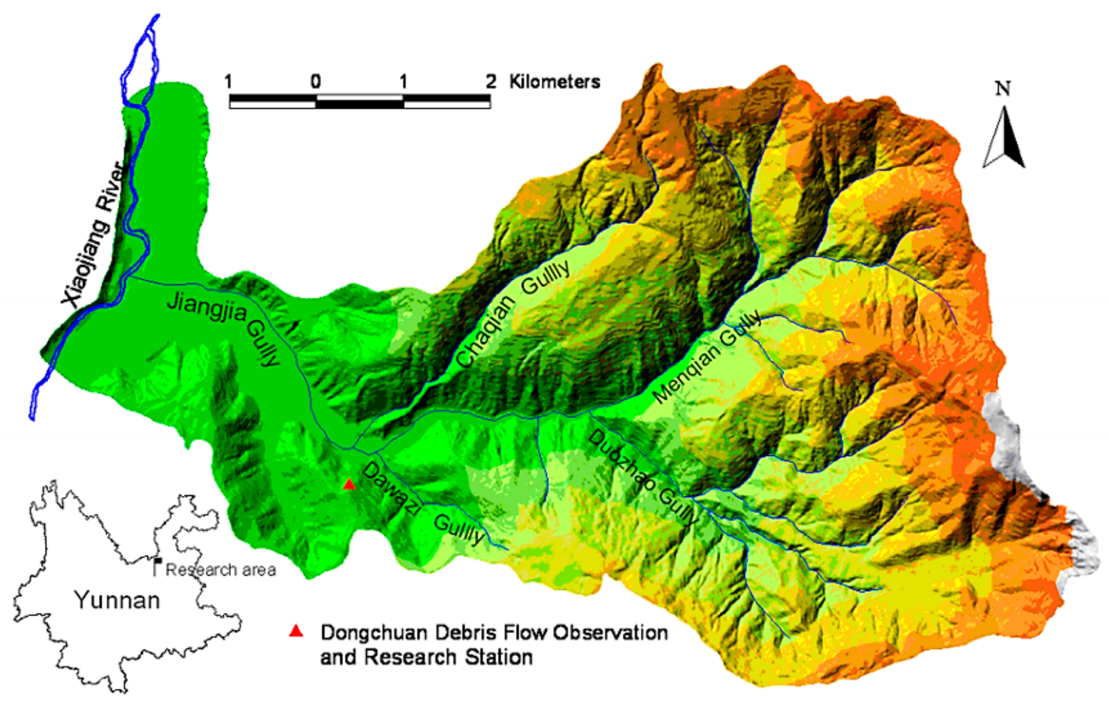
The loose debris was collected from the Jiangjiagou Valley which is located in Kunming City, Yunnan Province, China. Debris flows are common in this area, causing significant damages [41] and so the material collected is representative.
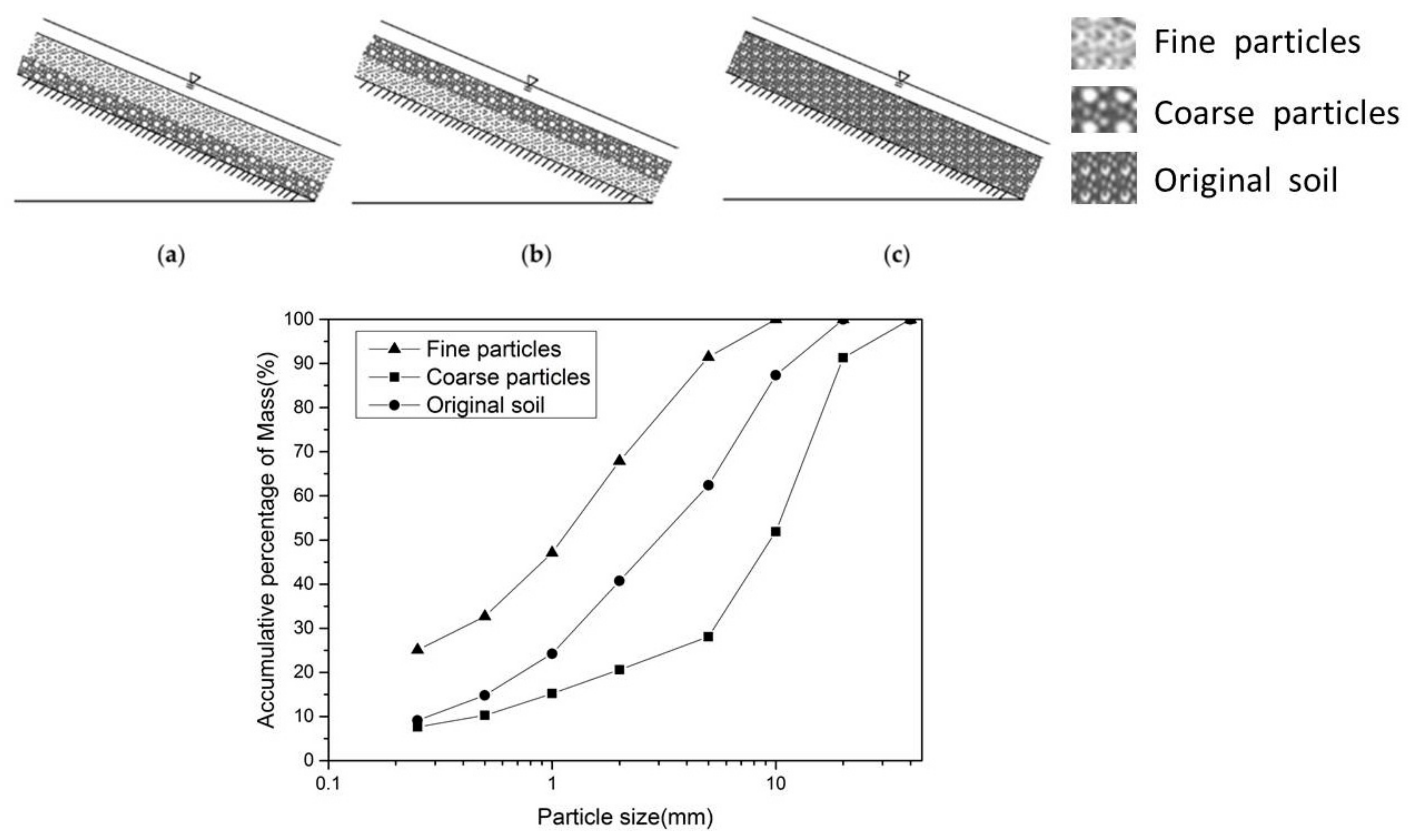
The experimental configurations chosen to examine the influence of vertical grading patterns on the debris flow formation and propagation are displayed in Figure 1. There are three configurations: Figure 1a shows the first configuration, with coarse particles as a bottom layer and fine sediment positioned above them; Figure 1b shows the second configuration, with coarse particles distributed on top of fine grains as a bottom layer; Figure 1c shows the third configuration, a realistic configuration with the original sediments collected from the Jiangjiagou Valley distributed along the entire measurement area. The first and second configurations separating coarse and fine particles were selected based on the three principles of vertical depositing patterns (i.e., normal, inverse grading and mixed) reported in earlier studies [38]. Figure 1 also includes the relevant particle size distribution curves for the material selected. In order to characterize the vertical grading, a coefficient (Ψ) was proposed as follows:
where d50up and d50down represent the median particle size of the upper and bottom layers, respectively. For this study, Ψ ranges between 0.11 and 8.43.
Steep topography, a high quantity of loose debris and runoff generated by either intense or low rainfall events are prerequisites for debris-flow occurrence. To replicate realistic scenarios initiated by these conditions, the following conditions were selected: the median grain size selected was d50; the coarse and fine particles were distributed in different vertical profiles; the scaled flow rates 6.5 and 19.5 m3/h were used; deposit morphology and channel width-depth ratio; and different flume slopes were selected to represent typical steepness of the watersheds in China (20° and 25°). The flow rates used were chosen as representative of flows quite similar to the natural flows recorded at the Debris Flow Observation and Research Station at Jiangjia Gully, in terms of bulk flow behaviour.
2.2. Experiments
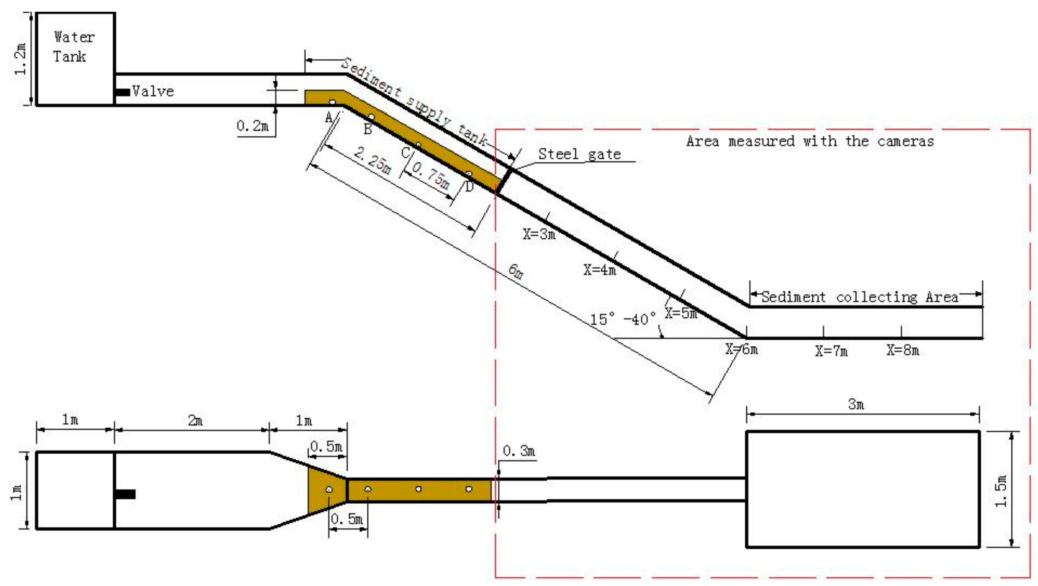
Experiments were performed in a 12.0 m long, 0.3 m wide, 0.4 m deep flume located in the Debris Flow Observation and Research Station at Jiangjia Gully, the largest field research centre in China—also known as “the debris flow museum” [42] (Figure 2). This facility (Figure 3) consists of a water tank (5.0 m above the laboratory floor which stores water up to 1.2 m3) fitted with a valve at its base, enabling the release of 6.5 m3/h when the valve is half opened and 19.5 m3/h when the valve is fully opened with an error measurement of ±5%. Between the flume and the water tank there is a debris supply tank followed by a steel gate. The flume can be divided into two parts: (i) a steep upstream reach (6.0 m long and the chute slope can vary from 15 to 40°); and (ii) a flat-bottomed downstream section (3.0 m long). The slope of the flume’s bed can be manually adjusted using 1° intervals.
Test details are listed in Table 1. In total, twelve tests were conducted in the experimental facility, combining different vertical grading, flow rates and flume slopes and reproducing all the configurations displayed in Figure 1.
Prior to each test run, the debris mixtures were carefully placed in the supply tank according to the vertical grading coefficient (Table 1 and Figure 1). The volume of solid debris placed in the supply tank was estimated to be around Vs ≈ 0.20 m3 and was maintained constant for each experiment. Half of this volume (0.10 m3) was filled with coarse particles and the other half (0.10 m3) was filled with fine particles for vertical grading configurations 1 and 2. The water pressure in the pores was recorded every second using pressure sensors buried in four locations at 0.3 H for all the hydraulic conditions tested to analyse the hydrodynamic characteristics of the non-homogeneous debris flow during the formation and propagation phases. (H is the height of the debris prior to testing). The pressure sensors used were PSI Pressure System Company (Hampton, VA, USA) model 730-13E-00005 pressure sensors. They have a measurement range of 0–1.5 m water, a precision of ±1 mm of water and an operating temperature range of 0–40 °C. These sensors were chosen to have a negligible effect on initial debris flow formation as they are quite small.
Velocities were also monitored to provide a better understanding of the propagation of the non-homogeneous debris flow and they were obtained by analysing videos recorded with two SONY ILCE-5100 high-speed cameras (Beijing, China), which were placed on each side of the flume (measurement area highlighted by a dash red line in Figure 3). These cameras provided a 1440 × 1080 pixel resolution video and captured a frame every 0.04 s. Grids, 10 × 5 cm2, were drawn along the propagation and accumulation areas of the flume on the glass windows on each side of the flume, so the velocity of the debris flow could be obtained by comparing the change of the fluid position of debris flow between frame intervals using Matlab. The videos were uploaded to Supplementary Materials. The error to estimated velocity values for this method corresponds to ±5%.
For the tests conducted, the following phenomena were observed after having opened the valve based on the corresponding flow rate to simulate:
- (i)
- movement of the sediments due to water movement infiltration with corresponding mixing of particles with different size and formation of debris flow;
- (ii)
- acceleration of debris flow to a maximum propagation velocity in the movement area;
- (iii)
- a rapid decrease of velocity when the debris flow reached the flat downstream area and finally accumulation and deposition in the downstream area.
These dynamic processes associated with non-homogeneous debris flows can be grouped into three different stages: formation, propagation and accumulation. The initial formation can be further divided into three other steps, the initial movement of smaller particles, their entrainment and acceleration and the final two-phase flow layering [6]. To identify the initial movement of the debris flow, the Shield’s number was taken as an indicator for this study. It can be quantified by using the following Equation (2):
where J is the hydraulic gradient (-); γ is the volumetric weight of water (Nm−3); γS is the solid bulk density of sediment particles (N/m−3); is the sediment Reynolds number (-), h is the water depth (m) and d is the particle size (m). The left-hand term is the relative shear force, the ratio between the drag force (N/m2) and the starting shear stress (N/m2) and its value is significant for determining whether the debris flow has initiated its movement [42]. When , the debris flow is initiated; when , the debris flow is in the critical initiation; and when the , debris flow has not initiated.
Finally, to make the results applicable to real case scenarios, useful for a wider range of applications, the Froude number was calculated for each test conducted [44,45].
By analysing and comparing all the parameters recorded and measured under different flow rates, slopes and vertical grading coefficients, the next sections present the degree of influence that all these factors have on the formation and the propagation of debris flows.
3. Results
This section presents an analysis of the variables collected (pore water pressure and averaged velocity) and the influence of the experimental conditions (different vertical grading, flow rates and flume slopes tested) on the formation and the propagation of debris flow replicated.
This study has been conducted to provide a better understanding of the relationship between the factors that could influence the three typical steps of debris flows: (i) the formation; (ii) the propagation and (iii) the accumulation. The formation process could be divided into three stages: (i) initiation; (ii) accelerated mixing of the solid particles and water; (iii) mixing particles with different size and formation of debris flow. The basic properties of three stages were analysed in the Section 3.1.
In order to complete a quantitative examination on the influence of different flow rates, slopes and vertical grading coefficients on debris flow formation and propagation, a regression analysis was conducted to estimate the relationship between all the experimental factors and the hydrodynamic characteristics. The regression analysis obtained in Section 3.2 is a predictive modelling technique typically used to study the relationship between dependent variables (targets) and independent variables (predictors) [45].
3.1. Experimental Properties of the Debris Flow Formation
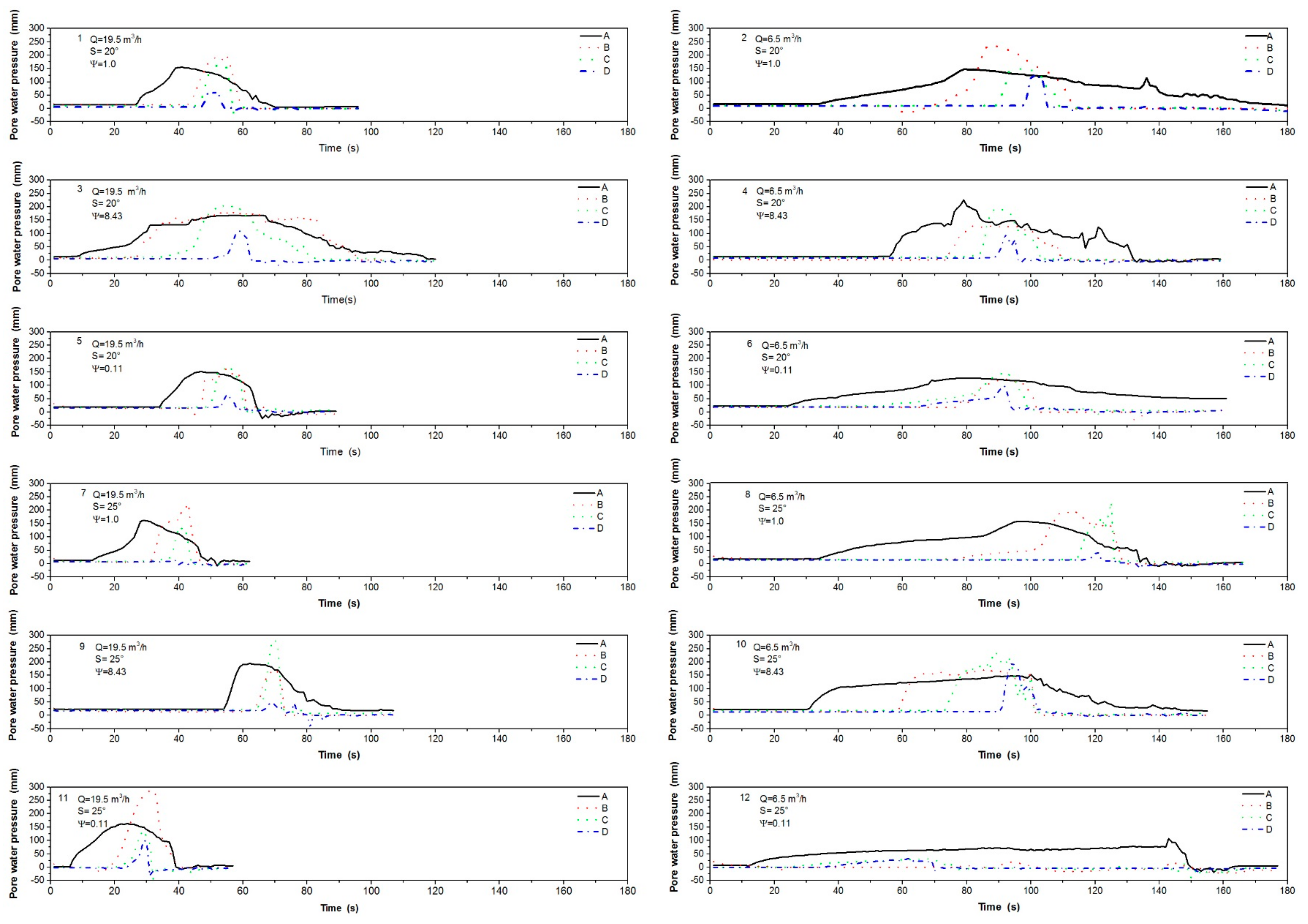
Equation (2) was applied to each test conducted and based on the criteria , it is possible in all the cases to confirm that the debris flow was initiated. The variations of pore water pressure under different flow rates are displayed in Figure 4. During the formation of the debris-flow, the data collected show that the pore water pressure gradually increased at the beginning of the formation process and then started to rapidly decrease. The water pore pressure became then stable and this hydraulic behaviour could be associated then to the initiation process of debris flow.
When the lower flow rate is applied, the curve obtained for the water pore pressure measured is more stretched and the peak pressure takes longer to be reached.
As described in Section 2.2, the experimental procedure was the same for each test conducted. The valve was opened to release the flow corresponding to each test for the entire test duration. Due to the different flowrates simulated and the different slopes used, some tests are longer than others. 180 s was the maximum duration encountered when conducting the experimental campaign for the sediments to be accumulated in the final zone (accumulation area).
Experiments displayed in Figure 4 include the three different vertical gradings shown in Figure 1 and the effects of grading can be compared by grouping those with similar initial flow rates released and similar slopes, such as in tests 7, 9 and 11.
The duration of formation of debris flow associated with test 7 (Ψ = 1.00) in locations A, B, C and D was 29 s, 43 s, 40 s and 39 s, respectively. Looking at the same parameter for another test with similar hydraulic conditions but different Ψ = 8.43, test 9, the duration of formation in each location A, B, C and D was 62 s, 70 s, 70 s and 76 s, respectively. For test 11 (Ψ = 0.11), the duration of formation was 24 s, 32 s, 30 s, 30 s, respectively. The same phenomenon was observed as well in another group of experiments (2, 4, 6) and, based on the comparison with the values of duration recorded, when the fine particles above the coarse particles configuration was applied, the formation process was the quickest. However, this behaviour was not observed for the remaining two experimental groups (1, 3, 5 and 8, 10, 12) demonstrating the effect of the slope (from 20 to 25°) in the debris flow formation.
By comparing the same group of tests with similar hydraulic conditions but different packing (7, 9 and 11 vs. 1, 3 and 5), it was possible to notice (as displayed in Figure 4) that when the slope is higher, the time to reach the peak of water pore pressure is faster for Ψ = 1.00 and Ψ = 0.11. This characteristic was not observed when comparing group (2, 4, 6) versus group (8, 10, 12), where the opposite behaviour was noticed, demonstrating an effect on the debris flow formation timing caused by the lower amount of flow rate released (6.5 m3/h).
Furthermore, for each experiment conducted, the pore water pressure constantly increased as the water gradually infiltrated through the sediments. When the initiation process was triggered, front-end particles first started to move followed by more particles, generating a bigger mass moving towards the same direction and facilitating the mixing of water and dry particles. The phase is illustrated in Figure 4 where the pore water pressure begins to slightly fluctuate after reaching the peak. Pore water pressure starting to rapidly decline could be defined as the mixing stage of debris with flow.
In Figure 4, comparing the tests with same flume slope and flow rate but different vertical grading, the duration of fluctuations in pore water pressure for the vertical grading Ψ = 8.43 with a lower flow rate was longer and the peak was longer than those associated with the other two vertical grading configurations. This phenomenon appeared as well for the groups of test 1, 3 and 5 and 2, 4 and 6. The duration of fluctuations in pore water pressure with the vertical grading Ψ = 0.11 under the higher flow rate (19.5 m3/h) was the longest when comparing for example tests 7, 9 and 11. This behaviour was observed to be similar for vertical grading Ψ = 0.11 for the group of tests 8, 10 and 12.
The mechanical properties of the soil in the formation area are different for the different vertical grading configurations because the stratification of dissimilar soils causes differences in the water pressure recorded. When the majority of the sediment particles located in the formation area have mixed with the water, the pore water pressure suddenly dropped, forming the two-phase debris flow.
By comparing experimental groups of tests with different flow rates but the same slope and vertical grading, it is possible to observe that the pore water pressure typically decreases much faster under the effect of large flow rate. This is visible in Figure 4. The decrease in pore water pressure associated with the two-phase flow layering process with a 20° slope was higher than that of the configuration with slope = 25°.
Based on the sketch of possible flow regimes (immature debris flow, mature debris flow—quasi uniform and mature debris flow accelerated) and occurrence criteria provided by Takahashi et al. (2007) [18] and applied by Lanzoni et al., 2017 [21], two flow regimes were observed in the tests, the immature debris flow and the mature-accelerated (sliding) debris flow with some tendency to landslide characteristics. When the first scenario was observed, a layer of clear water was noticed to be formed upon a flowing sediment-water mixture and the flow was not able to spread the sediment throughout the entire flow depth. For the second scenario, each test has been characterized by the formation of a front which was moving at an almost constant speed with a body of nearly constant depth, entailing a negligible erosion of the underlying sediment bed. This body then progressively elongated in time owing to sediment erosion in the upstream portion of the flume forming a tail where the entrainment of grains from the erodible bed were mainly concentrated.
3.2. Influence of Different Vertical Grading, Flow Rates and Flume Slopes on the Formation, the Propagation and the Intensity of Debris Flows
3.2.1. Initiation Time
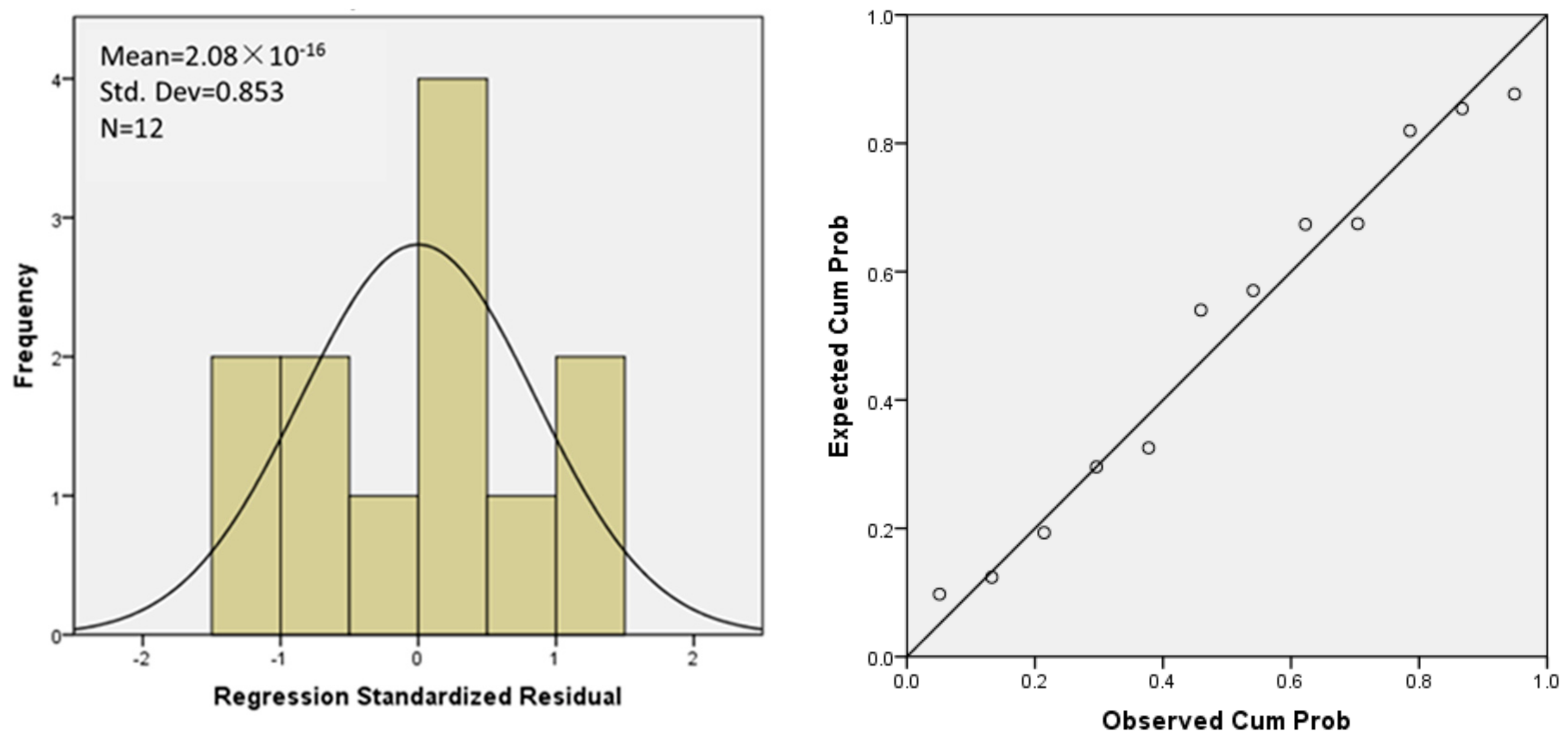
For this study, the regression equation to relate debris flow initiation time T and flow rate Q, slope S and the vertical grading coefficient Ψ can be represented as follows:
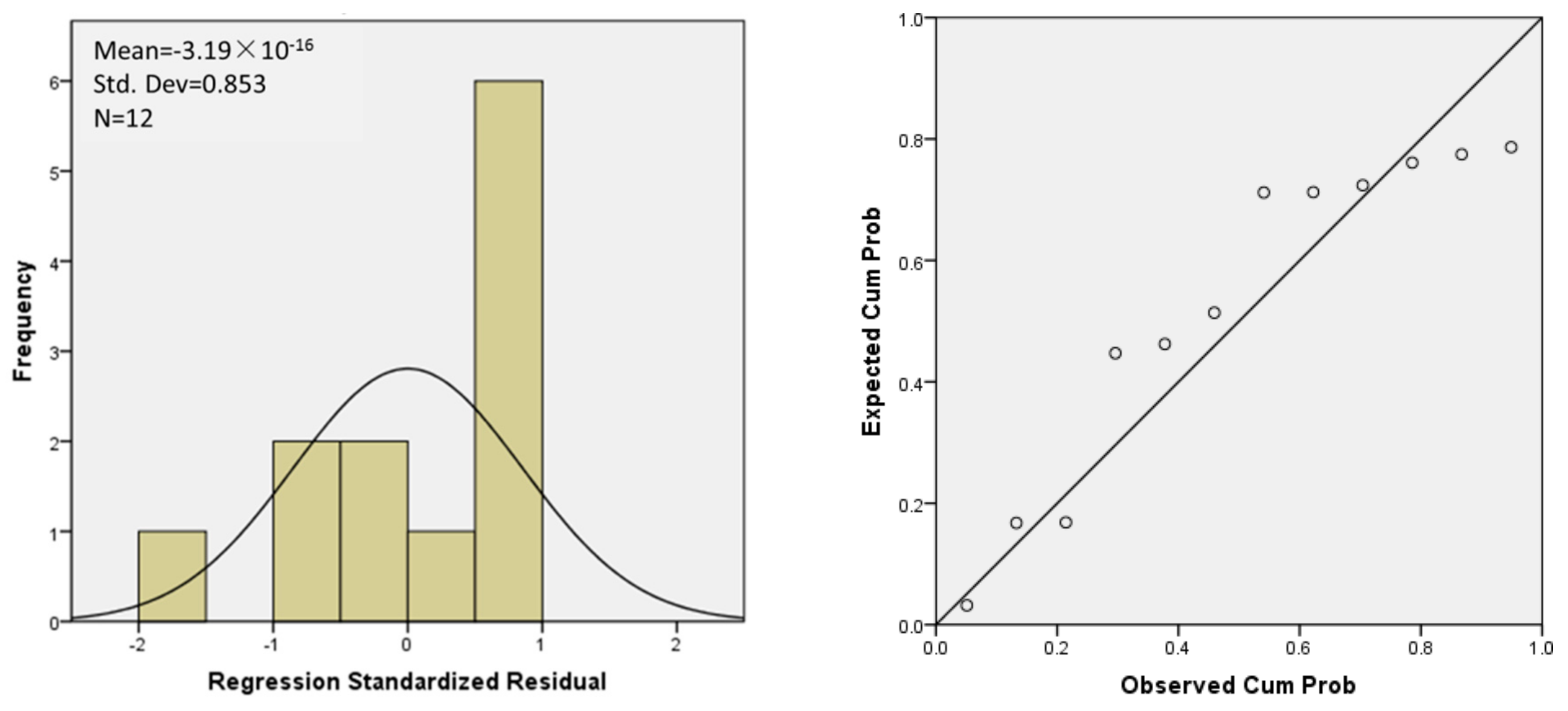
In order to verify the accuracy of the regression results, a regression diagnosis was needed. The diagnostic model ANOVA (Analysis of Variance) used for this study was the residual analysis technique. Standardized residual analysis histogram of SPSS (Statistical Product and Service Solutions) regression diagnostic and the standard P-P (Probability to Probability) chart are displayed in Figure 5. The results of the residual analysis confirmed that the histogram was a normal distribution, while the observed values in the P-P map could be fitted with the simulated values, showing that the regression equation obtained was applicable.
As three independent variables were considered for this research, the multiple regression method was employed to determine the correlation between a dependent output parameter and the continuous or discrete independent input parameters. According to the standard coefficients based on the regression, the contribution rate affecting the starting-time of the debris flow were ranked as presented in Table 2. The contribution rate of the flow rate on the process of initiation of the debris flow was 88.7%, hence it was ranked the first among the three variables selected. The contribution rate of the slope was 7.0% and the contribution rate of vertical grading coefficient was 4.2%.
The effect of flow rate on the formation area was mainly observed in the start-up time and the critical pore water pressure trend. High flow rates typically accelerated the initiation process and the mixing of the debris flow. On the contrary, the steepest slope shortened the start-up time, accelerating the mixing phase.
3.2.2. Propagation
The movement of the debris flow typically accelerates under the force of gravity [40]. High-speed debris flow can generate a very strong force which could cause serious damages when impacting against buildings, cars and people. Hence it is very important to be able to quantify it to provide a better understanding about its movement.
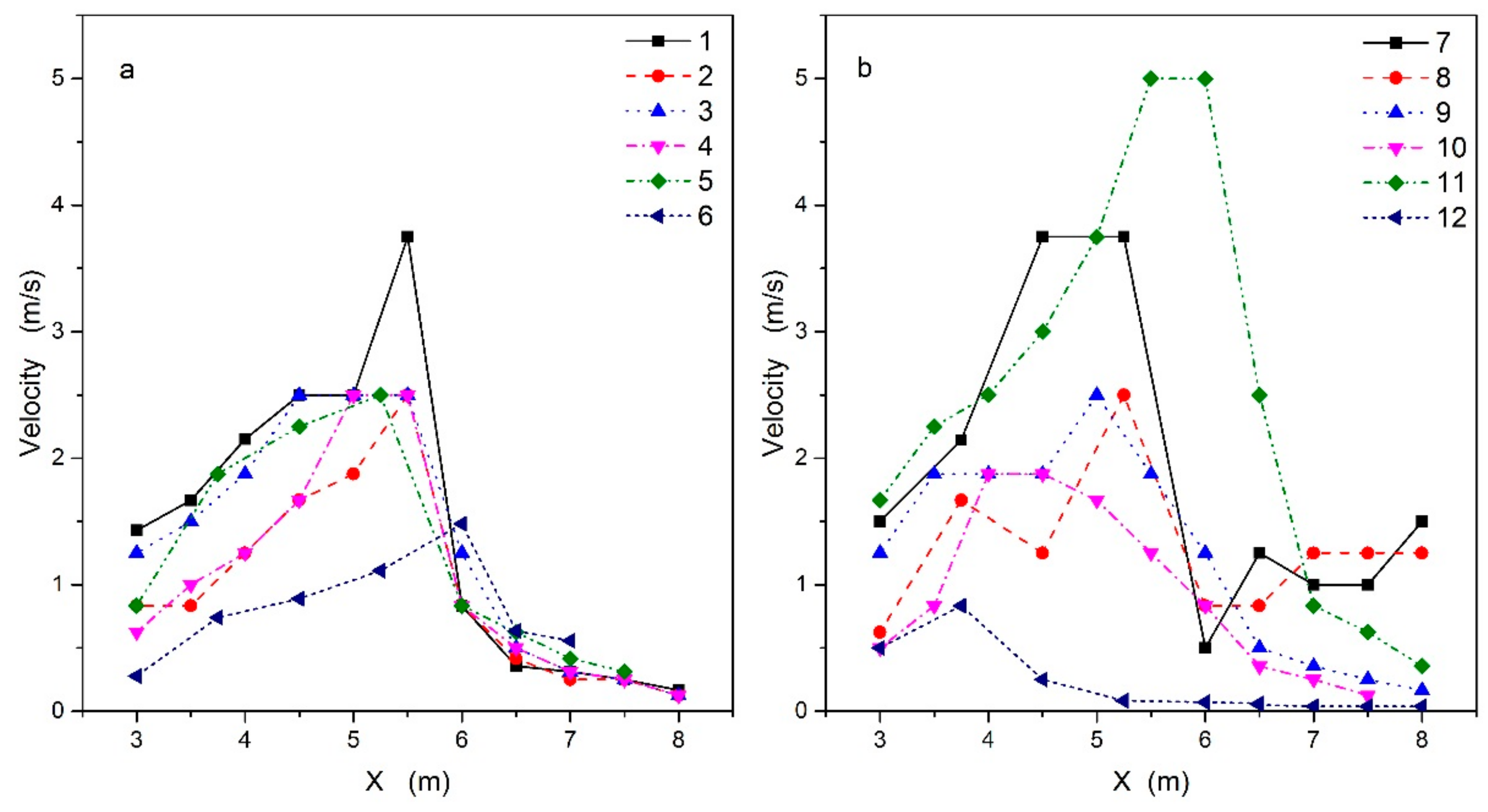
Velocity variation trends for all the hydraulic conditions simulated are similar when comparing tests with different flow rates (see Figure 6) but the corresponding magnitudes of velocity recorded were differing. For most of the tests, it has been observed that generally the clean water released at the beginning of the formation area gradually mixed with the solid particles, for then creating a mixture that accelerated and gradually increased in speed. After entering the movement area, the debris flow velocity increased rapidly, reaching the maximum value when approaching the end position of the accumulation zone and then slowing down when entering the accumulation area, due to resistance and friction until its velocity reached zero (complete dispersion). As expected, the velocity obtained for lower flow rate is smaller than the velocity obtained for higher flow rate.
It can be seen from Figure 6 that values of depth average velocities in different sections along the channel for each test (grouped by slope) follow similar patterns. In case of smaller slope (20°), the velocity has always been lower than that in the larger slope (25°).
The difference in Figure 6a between test 1, test 3 and test 5 showed that the variation of propagation velocity in debris flows caused by the difference of the vertical particle size distribution coefficient was not significant. The trend is similar to the difference between test 2, test 4 and test 6. It may be concluded from the simulation of the experiments that the configurations with different vertical grading had greater effect on the velocity of the movement process of debris flows when the flume slope was steeper.
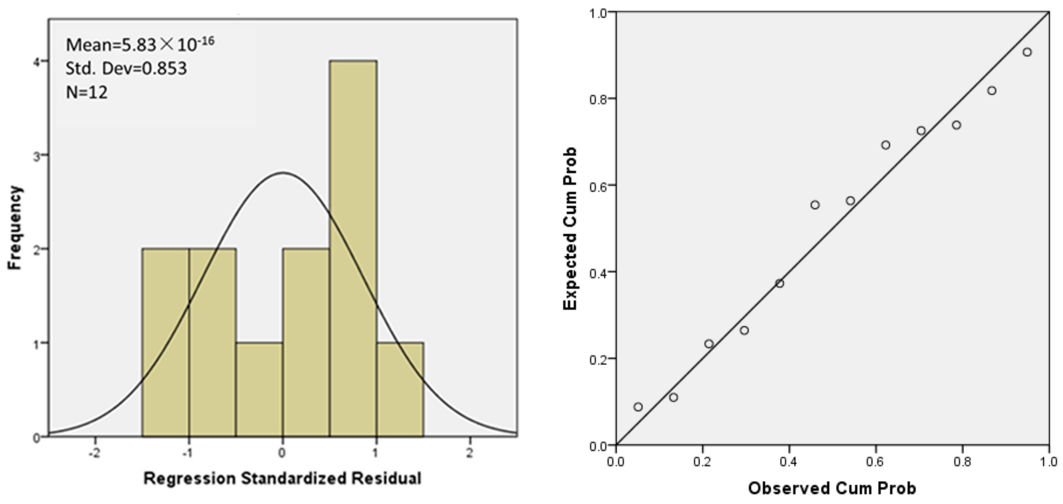
SPSS Regression Diagnostic Standardized Residual Analysis Histogram and Standard P-P chart obtained considering velocity values are displayed in Figure 7. The regression Equation (4) was obtained to calculate the debris flow average velocity by using flow rate Q, slope S and vertical grading coefficient Ψ as the dependent variables.
According to the result of residual analysis on the flow velocity in Table 3, the contribution of flow rate on average debris flow velocity is the largest at 98.9%. The contribution rate of the slope was 14.7% and this factor positively correlated with average flow velocity. The vertical grading coefficient negatively related to average flow velocity and its contribution rate was −13.5. Results also showed that the velocity associated with the propagation of the debris flows was higher for the configuration with fine particles located on the top of coarse particles when the flow released was 19.5 m3/h. However, when Q = 6.5 m3/h, tests with Ψ = 8.43 (Test 4, Test 10) have higher velocity than those with Ψ = 0.11 (Test 6, Test 12), respectively. Hence, in terms of velocity, it can be stated that the destructive force of debris flows can be higher and more powerful when the grain size distribution of the upper original soil is smaller than the subsoil’s one in combination with higher flow rates (19.5 m3/h > 6.5 m3/h).
3.2.3. Flow Intensity
Gravity and inertial forces are the main influences on debris flow propagation. To up-scale results obtained within the experimental facility, the Froude number (Equation (5)) was used to estimate the relationship between inertial forces and gravitational force for each experiment tested.
where v is the debris flow velocity (m/s), g is the gravitational acceleration (9.8 m/s2) and h is the debris flow depth (m).
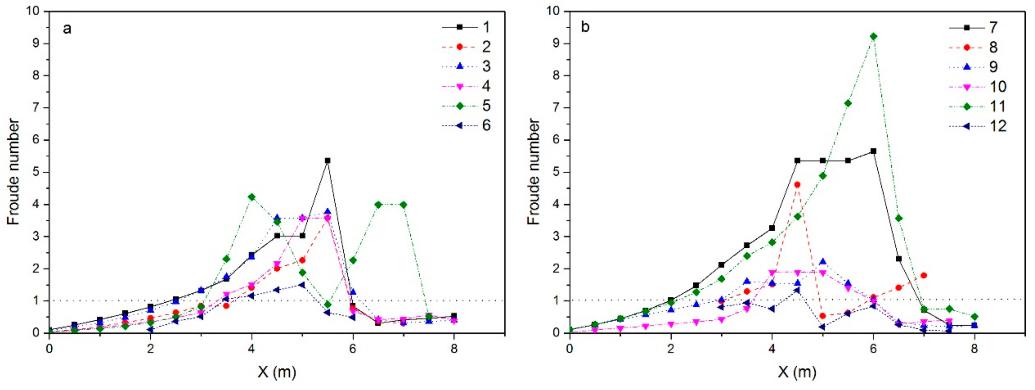
By comparing the variation of the Froude numbers for the entire movement of the non-homogeneous debris flow, using the same vertical grading and slope and changing the flow-rate used to induce the composition of the mixture, profiles obtained displayed in Figure 8 show similar trend despite different magnitudes.
As illustrated in Figure 8, Froude steadily increases reaching the maximum value in movement area at X = 5.5 m and then decreases rapidly approaching the accumulation zone. In the accumulation area, the flow rate slows down, the water level rises; and hence Froude increases slightly but remains below 1, until the flow stops. It can be noted that Fr > 1 for most of the processes except in the formation area and part of accumulation area (Figure 8).
By comparing Froude magnitude in the movement area for the configurations with slope 20° and 25° (test 3 and 9) but same hydraulic conditions, Froude is smaller for the 20° scenario. Test 9 includes the steepest slope but despite this the Froude number calculated is not the highest. The reason for this phenomenon is that the debris flow observed for test 9 acts as a landslide where the sediments glide down as a whole unit and the solid particles do not interact strongly with the water. Therefore, the flow intensity is smaller than the one typical of common debris flows.
The slope also has an effect on the strength of the flow. In general, if the slope is steeper the debris flow intensity is greater; on the other hand, if the slope is small the velocity intensity of debris flow is lower. As a consequence, if the mixing is less intense, the entire force of the solid matter in the debris flow declines.
The regression formula (Equation (6)) obtained to find Fr values using the three variables changed for the configuration of the tests (Q, S and Ψ), is listed as follows:
The corresponding standardized residual analysis histogram of SPSS regression diagnostic and standard P-P chart are illustrated in Figure 9.
According to the standard coefficient regression analysis obtained between the parameters and Froude number, the largest impact is due to the flow rate magnitude, characterized by a contribution rate of 84.4%. The slope has the second highest influence with 35.7% and the vertical grading coefficient is third with 20.0%. Flow rate and flume slope are positively correlated with Fr, while vertical grading coefficient has negative correlation. Details are shown in Table 4.
4. Conclusions
The dynamic characteristics associated with formation and propagation of debris flows were analysed based on the data collected during the experiments simulated (pore water pressure, velocity, Froude number). The conclusions can be summarized as follows:
- (1)
- The pore water pressure is the critical driving force to trigger the debris flow initiation. During the formation process of the debris flow, pore water pressure first gradually increase, reaches a peak and then declines rapidly. The critical initiated pore water pressure under the condition of small-scale flow released was lower than that the one recorded when released the higher flow rate. The initial growth rate of the pore water pressure was higher for the configuration where the fine particles were positioned above the coarse particles and the flume had the steepest slope. Focusing on the regression analysis of the factors influencing the formation process, the ranking list, from the most to the less influencing, of the three experimental parameters considered is given as: flow rate Q > flume slope S > vertical grading coefficient Ψ. Variables Q and S showed negative correlation with the formation time, which meant that the greater is the flow rate and the steeper is the slope, the shorter is the formation time.
- (2)
- When the pore water pressure begins to decrease rapidly, the debris flow enters the next phase—the movement process. The corresponding propagation velocity then reaches its maximum value. The ranked list based on the influences that the three variables have on the velocity magnitude can be rates as follows: flow rate Q > flume slope S > vertical grading coefficient Ψ. Flow rate and flume slope showed positive correlation with the velocity, while there is a negative correlation between the vertical grading coefficient and the velocity. The steeper the slope and the larger the original amount of water is, the higher is the movement of the debris flow. Additionally, the velocity of the debris flows is inversely proportional to the vertical grading coefficient.
- (3)
- Analysing the Froude number for the processes of formation and movement, it steadily rises and reaches its maximum value just at the end of the steep area, before reaching the accumulation zone. Fr values below 1 were obtained only in the formation zone and the end flat zone where the propagation of the debris flow was initiating and where the debris flow was reducing its speed, respectively. The Froude Number was larger than 1 in other areas, indicating the formation of supercritical flows associated with debris flow transport behaviour. The ranked list based on the influences that the three variables have on the Froude number can be rates as follows: flow rate Q > flume slope S > vertical grading coefficient Ψ. The higher the flow rate is and the steeper the flume is, the higher are Froude number values, while the higher vertical grading coefficient is, the lower are Froude number values.
The data collected are fundamental to providing a better understanding of debris flow formation and propagation and the results obtained can be used by numerical modellers to simulate this phenomenon and assist in the prevention and control of debris flows in China. However, the limitation of this study should be noted. The present investigation has been characterized only by a single trial for each combination of Q, S and Ψ, hence uncertainties associated with practical errors such as sediment disposition or accuracy of slope selected could not be properly estimated.
Future work should investigate the internal force of the debris flow with more experimental tests to improve additional information on the destructive internal force generated by the mixture of water and sediments, including the quantification of water content and debris flow depths. The particles-size distribution and the two-phase flow characteristics can be quantified. However, the internal force associated with debris flows includes multiple processes (e.g., the buoyancy of the sediments, the resistance of the sediments to the initiation, the friction between particles of different sediments, the change of yield stress and shear rate caused by water infiltration) and all these mechanisms are too complex to be analysed together hence a further detailed investigation is certainly required.
Supplementary Materials
The following are available online at https://zenodo.org/record/1215863#.WsyLS8mgnDw, Video S1: Test-1, Video S2: Test-2, Video S3: Test-3, Video S4: Test-4, Video S5: Test-5, Video S6: Test-6, Video S7: Test-7, Video S8: Test-8, Video S9: Test-9, Video S10: Test-10, Video S11: Test-11, Video S12: Test-12.
Acknowledgments
The research reported in this manuscript is funded by the Natural Science Foundation of China (Grant No. 11372048).
Author Contributions
All the authors jointly contributed to this research. An Ping Shu was responsible for the proposition and design of the experiments, analysis of the results and conclusions of the paper; Lu Tian and Matteo Rubinato analysed the experimental datasets and wrote the paper. Shu Wang, Fuyang Zhu, Mengyao Wang and Jiangtao Sun performed the experiments.
Conflicts of Interest
The authors declare no conflict of interest.
Notation
| Ψ | vertical gradient coefficient (-) |
| d50up | median particle size upper layer (mm) |
| d50down | median particle size lower layer (mm) |
| H | initial height debris (m) |
| J | hydraulic gradient (-) |
| γ | volumetric weight of water (Nm−3) |
| γS | solid bulk density of sediment particles (Nm−3) |
| sediment Reynolds number (-) | |
| h | water depth (m) |
| d | particle size (m) |
| drag force (N/m2) | |
| starting shear stress (N/m2) | |
| Q | flowrate (m3/h) |
| S | slope (°) |
| T | initiation time (s) |
| Fr | Froude number (-) |
| g | gravitational acceleration (m/s2) |
| h | debris flow depth (m) |
| v | velocity debris flow (m/s) |
References
- Iverson, R.M. Elementary theory of bed-sediment entrainment by debris flows and avalanches. J. Geophys. Res. Earth Surf. 2012, 117, 2156–2202. [Google Scholar] [CrossRef]
- McDougall, S.; Hungr, O. Dynamic modelling of entrainment in rapid landslides. Can. Geotech. J. 2005, 42, 1437–1448. [Google Scholar] [CrossRef]
- Rickenmann, D. Empirical relationships for debris flows. Nat. Hazards 1999, 19, 47–77. [Google Scholar] [CrossRef]
- Pitman, E.; Nichita, C.; Patra, A.; Bauer, A.; Bursik, M.; Weber, A. A model of granular flows over an erodible surface. Discrete Cont. Dyn. Syst. Ser. B 2003, 3, 589–600. [Google Scholar]
- Medina, V.; Hürlimann, M.; Bateman, A. Application of FLATModel, a 2D finite volume code, to debris flows in the northeastern part of the Iberian Peninsula. Landslides 2008, 5, 127–142. [Google Scholar] [CrossRef]
- Shu, A.P.; Wang, L.; Yang, K.A. Investigation on movement characteristics for non-homogeneous and solid-liquid two-phase debris flow. Chin. Sci. Bull. 2010, 55, 3006. [Google Scholar] [CrossRef]
- Zhou, Y.K.; Jin, X.B.; Wang, Q.; Du, X.D. Comprehensive assessment of natural disaster risk for agricultural production in Guanzhong region based on GIS. Sci. Geogr. Sin. 2012, 32, 1465–1472. [Google Scholar]
- Fei, X.; Shu, A. Debris Flow Movement Mechanism and Disaster Prevention; Tsinghua University Press: Beijing, China, 2004. [Google Scholar]
- Cui, P. Progress and prospects in research on mountain hazards in China. Progress Geogr. 2014, 33, 145–152. [Google Scholar]
- Xu, Z.; Huang, R. The response of the groundwater in vegetated slopes mountainous catchments to heavy rate events. Adv. Earth Sci. 2011, 26, 598–607. [Google Scholar]
- Yu, B.; Ma, Y.; Zhang, J.; Li, L.; Chu, S.; Qi, X. The group debris flow hazards after the Wenchuan Earthquake in Longchi, Dujiangyan, Sichuan province. J. Mt. Sci. 2011, 29, 738–746. [Google Scholar]
- Nettleton, I.M.; Martin, S.; Hencher, S.; Moore, R. Debris Flow Types and Mechanisms. 2007. Available online: http://www.geoffice.it/files/Download/0015327.pdf (accessed on 19 December 2017).
- Heald, A.; Parsons, J. Key contributory factors to debris flows. In Scottish Road Network Landslides Study; Winter, M.G., Macgregor, F., Shackman, L., Eds.; The Scottish Executive: Edinburgh, UK, 2005; pp. 68–80. Available online: http://www.scotland.gov.uk/Publications/2005/07/08131738/17395 (accessed on 19 December 2017).
- Highland, L.; Bobrowsky, P.T. The Landslide Handbook: A Guide to Understanding Landslides; US Geological Survey: Reston, VA, USA, 2008; p. 129. Available online: http://pubs.usgs.gov/circ/1325/ (accessed on 19 December 2017).
- Calligaris, C.; Zini, L. Debris flow phenomena: A short overview? In Earth Sciences; Dar, I.A., Ed.; InTech Publisher: Rijeka, Croatia, 2012; pp. 71–90. Available online: http://cdn.intechopen.com/pdfs-wm/27588.pdf (accessed on 21 December 2017).
- Shu, A.; Sun, J.; Xin, Z.; Shu, W.; Shi, Z.; Pan, H. Dynamical characteristics of formation processes for non-homogeneous debris flow. J. Hydraul. Eng. 2016, 47, 850–857. [Google Scholar]
- Bagnold, R.A. Experiments on a gravity-free dispersion of large solid spheres in a Newtonian fluid under shear. Proc. R. Soc. Lond. 1954, 225A, 49–63. [Google Scholar] [CrossRef]
- Takahashi, T. Debris Flow: Mechanics, Prediction and Counter-Measures; Taylor and Francis: New York, NY, USA, 2007. [Google Scholar]
- Luca, I.; Tai, Y.C.; Kuo, C.Y. Modeling shallow gravity-driven solid-fluid mixtures over arbitrary topography. Commun. Math. Sci. 2009, 7, 1–36. [Google Scholar]
- Qian, N.; Wang, Z. A Preliminary study on the mechanism of debris flows. J. Geogr. 1984, 39, 33–43. [Google Scholar]
- Lanzoni, S.; Gregoretti, C.; Stancanelli, L.M. Coarse-grained debris flow dynamics on erodible beds. J. Geophys. Res. Earth Surf. 2017, 122, 592–614. [Google Scholar] [CrossRef]
- Johnson, A.M.; Rahn, P.H. Mobilization of debris flows. J. Geomorphol. 1970, 9, 168–186. [Google Scholar]
- Stancanelli, L.M.; Lanzoni, S.; Foti, E. Propagation and deposition of stony debris flows at channel confluences. Water Resour. Res. 2014, 51, 5100–5116. [Google Scholar] [CrossRef]
- Stancanelli, L.M.; Lanzoni, S.; Foti, E. Mutual interference of two debris flow deposits delivered in a downstream river reach. J. Mt. Sci. 2014. [CrossRef]
- Ni, J.; Wang, G.; Zhang, H. The Basic Theory of Solid—Liquid Two—Phase Flow and Its Latest Application; Science Press: Beijing, China, 1991. [Google Scholar]
- Zhou, W.; Tang, C. Rainfall thresholds for debris flows occurrence in the Wenchuan earthquake area. Adv. Water Sci. 2013, 24, 786–793. [Google Scholar]
- Bin, Y.U.; Yuan, Z.; Tao, W.; Yunbo, Z. Research on the 10-minute rainfall prediction model for debris flows. Adv. Water Sci. 2005, 26, 347–355. [Google Scholar]
- Xu, L.; Wang, Q.; Chen, J. Forcast for average velocity of debris flow based on BP neural network. J. Jilin Univ. 2013, 43, 186–191. [Google Scholar]
- Savage, S.B.; Hutter, K. The motion of a finite mass of granular material down a rough incline. J. Fluid Mech. 1989, 199, 177–215. [Google Scholar] [CrossRef]
- Pusadaini, S.P.; Hutter, K. Rapid shear flows of dry granular masses down curved and twisted channels. J. Fluid Mech. 2003, 495, 193–208. [Google Scholar]
- Zahibo, N.; Pelinovsky, E.; Talipova, T.; Nikolkina, I. Savage-Hutter model for avalanche dynamics in inclined channels: Analytical solutions. J. Geophys. Res. 2010, 115. [Google Scholar] [CrossRef]
- Che, C.L. Generalized viscoplastic modelling of debris flow. J. Hydraulic Research 1988, 114, 237–258. [Google Scholar]
- Iverson, R.M. The physics of debris flows. Rev. Geophys. 1997, 35, 242–296. [Google Scholar] [CrossRef]
- Iverson, R.M.; Denlinger, R.P. Flow of variably fluidized granular masses across three-dimensional terrain: 1. Coulomb mixture theory. J. Geophys. Res. 2001, 106, 537–552. [Google Scholar] [CrossRef]
- Pudasaini, S.P.; Wang, Y.; Hutter, K. Modelling debris flows down general channels. Nat. Hazard Earth Syst. Sci. 2005, 5, 799–819. [Google Scholar] [CrossRef]
- Fernndez-Nieto, E.D.; Bouchut, F.; Bresh, D.; Castro Diaz, J.; Mangeney, A. A new Savage-Hutter type model for submarine avalanches and generated tsunami. J. Comput. Phys. 2008, 227, 7720–7754. [Google Scholar] [CrossRef]
- Pitman, E.B.; Le, L. A two-fluid model for avalanche and debris flows. Phyl. Trans. R. Soc. Lond. 2005, 363, 1573–1602. [Google Scholar] [CrossRef] [PubMed]
- Shu, A.; Wang, L.; Zhang, X.; Qiang, G.; Wang, S. Study on the formation and initial transport for non-homogeneous debris flow. Water 2017, 9, 253. [Google Scholar] [CrossRef]
- Takahashi, T. Debris Flow, Monograph of IAHR; AA Balkema: Rotterdam, The Netherlands, 1991. [Google Scholar]
- Jakob, M.; Hungr, O. Debris-Flow Hazards and Related Phenomena; Earth Science & Geography; Springer: Berlin/Heidelberg, Germany, 2005; ISBN 978-3-540-27129-1. [Google Scholar]
- Chen, X.Q.; Cui, P.; Feng, Z.L.; Chen, J.; Li, Y. Artificial rainfall experimental study on landslide translation to debris flow. Chin. J. Rock Mech. Eng. 2006, 25, 106–116. [Google Scholar]
- Shu, A.; Zhang, X.; Duan, G. Distinguish relations for the critical intitiation of non-homogeneous debris flow. J. Hydraul. Eng. 2017, 48, 757–764. [Google Scholar]
- Peng, H.; Zhao, Y.; Cui, P.; Zhang, W.; Chen, X.; Chen, X. Two-dimensional numerical model for debris flows in the Jiangjia Gully, Yunnan Province. J. Mt. Sci. 2011, 8, 757–766. [Google Scholar] [CrossRef]
- Hu, K.; Hu, C.; Li, Y.; Cui, P. Characteristics and mechanisms of debris-flow surges at Jiangjia Ravine. Ital. J. Eng. Geol. Environ. 2011. [Google Scholar] [CrossRef]
- Chen, S.C.; Ferng, J.W.; Wang, Y.T. Assessment of disaster resilience capacity of hillslope communities with high risk for geological hazards. Eng. Geol. 2008, 98, 86–101. [Google Scholar] [CrossRef]
Figure 1.
Particle size distribution curves typical of the material used for this study and schematic representation of the vertical distribution of coarse and fine particles within three experimental debris configurations. (a) normal grading with Ψ = 0.11; (b) inverse grading with Ψ = 8.43; (c) homogeneous grading pattern with Ψ = 1.0.

Figure 2.
Location of Jiangjia Gully Basin. The triangle represents the Dongchuan Debris Flow Observation and Research Station (DDFORS) (© [43]).
Figure 2.
Location of Jiangjia Gully Basin. The triangle represents the Dongchuan Debris Flow Observation and Research Station (DDFORS) (© [43]).

Figure 3.
Schematic of the experimental flume. The measurement area recorded by the cameras is highlighted by a dash red line.
Figure 3.
Schematic of the experimental flume. The measurement area recorded by the cameras is highlighted by a dash red line.

Figure 4.
The variation curve of pore water pressure in each experiment conducted.

Figure 5.
Residual analysis results for debris flow initiation time T vs. flow rate Q, slope S and the vertical grading coefficient Ψ.
Figure 5.
Residual analysis results for debris flow initiation time T vs. flow rate Q, slope S and the vertical grading coefficient Ψ.

Figure 6.
Velocity measurements for all the different experiments conducted. (a) shows the velocity along the channel for each test when the slope of the flume was 20°, (b) shows the velocity along the channel for each test when the slope of the flume was 25°.
Figure 6.
Velocity measurements for all the different experiments conducted. (a) shows the velocity along the channel for each test when the slope of the flume was 20°, (b) shows the velocity along the channel for each test when the slope of the flume was 25°.

Figure 7.
Residual analysis results for debris flow average velocity V vs. flow rate Q, slope S and the vertical grading coefficient Ψ.
Figure 7.
Residual analysis results for debris flow average velocity V vs. flow rate Q, slope S and the vertical grading coefficient Ψ.

Figure 8.
Froude number values obtained for all the experiments conducted. (a) shows the Froude number values for each test when the slope of the flume was 20°, (b) shows the Froude number values for each test when the slope of the flume was 25°.
Figure 8.
Froude number values obtained for all the experiments conducted. (a) shows the Froude number values for each test when the slope of the flume was 20°, (b) shows the Froude number values for each test when the slope of the flume was 25°.

Figure 9.
Residual analysis results for Froude Number Fr vs. flow rate Q, slope S and the vertical grading coefficient Ψ.
Figure 9.
Residual analysis results for Froude Number Fr vs. flow rate Q, slope S and the vertical grading coefficient Ψ.


Table 1.
Experimental testing conditions.
| Group | Test ID | Flow Rate Q (m3/h) | Vertical Grading Coefficient Ψ | Flume Slope S (°) |
|---|---|---|---|---|
| 1 | 1 | 19.5 | 1.00 | 20° |
| 2 | 6.5 | 1.00 | 20° | |
| 3 | 19.5 | 8.43 | 20° | |
| 4 | 6.5 | 8.43 | 20° | |
| 5 | 19.5 | 0.11 | 20° | |
| 6 | 6.5 | 0.11 | 20° | |
| 2 | 7 | 19.5 | 1.00 | 25° |
| 8 | 6.5 | 1.00 | 25° | |
| 9 | 19.5 | 8.43 | 25° | |
| 10 | 6.5 | 8.43 | 25° | |
| 11 | 19.5 | 0.11 | 25° | |
| 12 | 6.5 | 0.11 | 25° |
Table 2.
Contribution rates of experimental factors on starting time.
| Rank | Influence Factor | Standard Coefficient | Contribution Rate | Accumulative Contribution Rate |
|---|---|---|---|---|
| 1 | Flow rate | −0.864 | 0.887 | 0.887 |
| 2 | Flume Slope | −0.069 | 0.070 | 0.957 |
| 3 | Vertical grading coefficient | −0.041 | 0.042 | 1.000 |
Table 3.
Contribution rates of experimental factors on average flow velocity.
| Rank | Influence Factor | Standard Coefficient | Contribution Rate | Accumulative Contribution Rate |
|---|---|---|---|---|
| 1 | Flow rate | 0.817 | 0.989 | 0.989 |
| 2 | Flume Slope | 0.121 | 0.147 | 1.135 |
| 3 | Vertical grading coefficient | −0.112 | -0.135 | 1.000 |
Table 4.
Contribution rates of experimental factors on Froude Number.
| Rank | Influenced Parameters | Standard Coefficient | Contribution Rate | Accumulative Contribution Rate |
|---|---|---|---|---|
| 1 | Flow rate | 0.626 | 0.844 | 0.844 |
| 2 | Flume Slope | 0.265 | 0.357 | 1.200 |
| 3 | Vertical grading coefficient | −0.149 | −0.200 | 1.000 |
© 2018 by the authors. Licensee MDPI, Basel, Switzerland. This article is an open access article distributed under the terms and conditions of the Creative Commons Attribution (CC BY) license (http://creativecommons.org/licenses/by/4.0/).
Share and Cite
MDPI and ACS Style
Shu, A.P.; Tian, L.; Wang, S.; Rubinato, M.; Zhu, F.; Wang, M.; Sun, J. Hydrodynamic Characteristics of the Formation Processes for Non-Homogeneous Debris-Flow. Water 2018, 10, 452. https://doi.org/10.3390/w10040452
AMA Style
Shu AP, Tian L, Wang S, Rubinato M, Zhu F, Wang M, Sun J. Hydrodynamic Characteristics of the Formation Processes for Non-Homogeneous Debris-Flow. Water. 2018; 10(4):452. https://doi.org/10.3390/w10040452
Chicago/Turabian StyleShu, An Ping, Lu Tian, Shu Wang, Matteo Rubinato, Fuyang Zhu, Mengyao Wang, and Jiangtao Sun. 2018. "Hydrodynamic Characteristics of the Formation Processes for Non-Homogeneous Debris-Flow" Water 10, no. 4: 452. https://doi.org/10.3390/w10040452
Note that from the first issue of 2016, this journal uses article numbers instead of page numbers. See further details here.