Estimating the Optical Properties of Inorganic Matter-Dominated Oligo-to-Mesotrophic Inland Waters
by
 , , ,
, , ,
Thanan Rodrigues
1,* ,
,
Deepak R. Mishra
2,
Enner Alcântara
3,
Ike Astuti
4,
Fernanda Watanabe
1 and
Nilton Imai
1 1
Department of Cartography, Faculty of Sciences and Technology, São Paulo State University (UNESP), Rua Roberto Simonsen 305, Presidente Prudente 19060-900, SP, Brazil
2
Department of Geography, Center for Geospatial Research, University of Georgia (UGA), Athens, GA 30602, USA
3
Department of Environmental Engineering, Institute of Science and Technology, São Paulo State University (UNESP), Rodovia Presidente Dutra Km 137.8, São José dos Campos 12247-004, SP, Brazil
4
Department of Geography, State University of Malang (UM), Jl. Semarang 5, Malang 65145, Indonesia
*
Author to whom correspondence should be addressed.
Water 2018, 10(4), 449; https://doi.org/10.3390/w10040449
Submission received: 20 March 2018
/
Revised: 31 March 2018
/
Accepted: 3 April 2018
/
Published: 9 April 2018
(This article belongs to the Section Water Quality and Contamination)
Abstract
:Many studies over the years have focused on bio-optical modeling of inland waters to monitor water quality. However, those studies have been conducted mainly in eutrophic and hyper-eutrophic environments dominated by phytoplankton. With the launch of the Ocean and Land Colour Instrument (OLCI)/Sentinel-3A in 2016, a range of bands became available including the 709 nm band recommended for scaling up these bio-optical models for productive inland waters. It was found that one category of existing bio-optical models, the quasi-analytical algorithms (QAAs), when applied to colored dissolved organic matter (CDOM) and detritus-dominated waters, produce large errors. Even after shifting the reference wavelength to 709 nm, the recently re-parameterized QAA versions could not accurately retrieve the inherent optical properties (IOPs) in waterbodies dominated by inorganic matter. In this study, three existing versions of QAA were implemented and proved inefficient for the study site. Therefore, several changes were incorporated into the QAA, starting with the re-parameterization of the empirical steps related to the total absorption coefficient retrieval. The re-parameterized QAA, QAAOMW showed a significant improvement in the mean absolute percentage error (MAPE). MAPE decreased from 58.05% for existing open ocean QAA (QAALv5) to 16.35% for QAAOMW. Considerable improvement was also observed in the estimation of the absorption coefficient of CDOM and detritus from a MAPE of 91.05% for QAALv5 to 18.87% for QAAOMW. The retrieval of the absorption coefficient of phytoplankton () using the native form of QAA proved to be inaccurate for the oligo-to-mesotrophic waterbody due to the low returning negative predictions. Therefore, a novel approach based on the normalized was adopted to maintain the spectral shape and retrieve positive values, resulting in an improvement of 119% in QAAOMW. Further tuning and scale-up of QAAOMW to OLCI bands will aid in monitoring water resources and associated watershed processes.
1. Introduction
The inland waters represented by rivers, lakes, and reservoirs play a key role in the hydrological cycle providing different habitats and ecosystem services [1]. As many other ecosystems, inland waters have been under increasing anthropogenic or developmental pressure from industry, agriculture, and urban activities, increasing nutrient loading and other organic and inorganic pollution [2]. Infusion of nutrients (nitrogen (N) and phosphorus (P)) from the land via runoff often leads to eutrophication increasing the primary production of phytoplankton and macrophytes [3]. In oligo-to-mesotrophic reservoirs, the submersed species of macrophytes, which are usually rooted, occupy the edges and often the slow-moving zones of rivers [4]. They are dependent on the sediment supply and light availability for their optimal growth [5]. The clarity of the water is affected by the turbidity generated from sediments or other suspended particles, algae, and dissolved matter [6]. Frequent spatiotemporal monitoring of the physical, chemical, and biological constituents is of great importance for monitoring point and non-point source pollution for effective lake and reservoir management. Brazilian inland waters are being adversely affected by increased runoff originating from anthropogenic activities, such as expansions in agriculture and urban centers. They are still being managed using traditional methods such as in situ point sampling and lab analysis, which often fail to provide information about the spatiotemporal variability of water constituents. Due to the synoptic view and periodicity provided by the orbital sensors, remote sensing is considered an appropriate method for monitoring water quality, although the accuracy of bio-optical models for inland waters is still a challenge.
Yacobi et al. and Odermatt et al. [7,8] highlighted the main scientific challenges in studying complex waters using remote sensing. The variability within these types of waters in terms of concentrations, as well as specific inherent optical properties (SIOPs) of chlorophyll-a (Chl-a), suspended particulate matter (SPM), and colored dissolved organic matter (CDOM), can be difficult to separate. On the contrary, in the open ocean, the concentrations of non-algal particles (NAP) and CDOM are directly correlated with phytoplankton [9]. This means that at certain wavelengths, such as blue and green, it is possible to retrieve Chl-a concentrations in the open ocean but in inland waters, it can be highly erroneous because CDOM and NAP have strong overlapping absorption, particularly in the blue spectral region. To address this issue, much effort has been given to understanding the bio-optical properties of inland waters in order to retrieve the optically significant constituents (OSCs: Chl-a, SPM, NAP, and CDOM) by using inversion models based on empirical and analytical approaches [10,11]. In general, the inversion models first derive the inherent optical properties (IOPs) using the in situ measured apparent optical property (AOP) and then retrieve the OSC concentration [12].
Empirical models retrieve the water quality parameters by statistical relationships between an AOP, such as the remote sensing reflectance () or the irradiance reflectance (R), and a known OSC [13,14,15]. The method can be time and site limited and it is not related to any physical principle [16]. The semi-analytical and quasi-analytical (QAA) algorithms are based on radiative transfer theory and often include some empirical steps [8,11,17,18]. A semi-analytical algorithm estimates the total absorption coefficient () by the sum of the absorption coefficients of phytoplankton (), CDOM (), and NAP (), while QAA estimates using alone. A semi-analytical algorithm also estimates a backscattering coefficient () by summing the backscattering of each in-water constituent except for CDOM while the QAA retrieves [19].
The original QAA by [20] was developed to retrieve absorption and backscattering properties in the open ocean and coastal waters and later re-parameterized for turbid inland waters [21,22,23]. The model follows several steps mixing empirical and analytical approaches to derive the IOPs using radiative transfer equations, considering the reference wavelength () at 555 nm [20] (Table 1). At this wavelength, the contribution of SPM is very high in turbid eutrophic waters, which requires to be shifted to longer wavelengths such as 710 nm [21], 754 nm [22], and 708 nm [23,24]. Lee et al. [20] also showed the performance of QAA using 640 nm as and noticed considerable improvement for high-absorption environments where is higher than 0.3 m−1. However, Le et al. [21] emphasized the importance of more validation to improve the performance of this approach. In mesotrophic inland waters, Yacobi et al. [7] highlighted that for wavelengths longer than 600 nm, increases over other OSCs, which means that at shorter wavelengths the contribution of other OSCs, except water, is decreasing the performance of QAA.
The performance of QAAs for inland waters has been tested in various studies using the center bands from the medium resolution imaging spectrometer (MERIS), which is not operational now; however, the sites considered were all highly turbid and productive inland waters. For instance, Le et al. [21] studied the turbid Taihu Lake with a Chl-a concentration ranging between 3.07 and 299.60 mg m−3, Yang et al. [22] studied three turbid Asian lakes with Chl-a varying between 9.79 and 153.92 mg m−3, and Mishra et al. [23] explored the performance of QAA in aquaculture ponds dominated by cyanobacteria with Chl-a ranging between 95.68 and 1376.57 mg m−3 and accounting for 54% of . The main modification carried out by these studies, besides shifting to the near-infrared (NIR), was in the estimation of the spectral slope of particle backscattering (η).
With the launch (16 February 2016) of the Ocean and Land Colour Instrument (OLCI) onboard Sentinel-3A (OLCI/Sentinel-3A), a broader range of spectral bands became available mainly for applications in inland waters where the contribution of SPM in longer wavelengths is still present. Watanabe et al. [25] modified the original empirical steps of QAA from Lee et al. [26] to estimate the IOPs in an inland water dominated by phytoplankton and then shifted the to 709 nm, achieving an average normalized root mean square error (NRMSE) of 21.88% for . Their results confirmed the suitability of a band at 709 nm to study inland waters, which means that the OLCI can be a powerful instrument for water quality monitoring considering inland waters. These findings have opened a new frontier for QAA applications based on re-parameterizations for inland waters. However, there is still a lack of research related to non-productive inland waters with dominated by CDOM and NAP and not by phytoplankton. Therefore, we hypothesized that even with the OLCI band at 709 nm (width of 10 nm), the accuracy of the IOP retrieval will be compromised by the version of QAA chosen, which means that the empirical steps should be locally tuned to increase its accuracy. This is justified because the inorganic matter presented in our study site can increase the reflectance in the NIR spectral region affecting the QAA accuracy. For that reason, this study aimed at evaluating the performance and potential of the OLCI/Sentinel-3A in retrieving the IOPs in a non-productive tropical reservoir. The specific objectives were (i) to validate three different approaches for QAA in non-productive inland water; (ii) to re-parameterize key steps of QAA using field data typical of non-turbid inland water and validate the model using an independent dataset; (iii) to replace the original steps associated with estimation for non-productive inland waters and propose an alternative method in order to avoid negative predictions; (iv) to link the QAA-derived IOP variability to physical and meteorological conditions; and (v) to characterize the factors that affect the bio-optical properties.
2. Materials and Methods
2.1. Study Area
Nova Avanhandava (Nav) is a run-of-river reservoir with a mean water level fluctuation lower than 0.50 m/year [27] (Figure 1). Nav is also the fifth of six reservoirs situated along the Tietê River in the west region of São Paulo State, Brazil, and started its activity in 1982, flooding an area of 210 km² (at its maximum quota), with a usable volume of 2.83 × 10⁶ m3, perimeter of 462 km, maximum depth of 30 m, mean residence time of water of about 46 days, and an average flow of 688 m3 s−1 [28].
Nav is an oligo-to-mesotrophic reservoir with the upper layer of the water column well oxygenated and pH ranging from slightly acid to alkaline (6.47–8.2), conductivity relatively high (83–150 µS cm−1), and low concentrations of nutrients (total N 0.05–0.23 µg L−1 and total P 18.02–32.33 µg L−1) [29,30]. The high transparency of the water often leads to the growth of submerged macrophytes (e.g., Egeria sp.) [30], although during sample collections we avoided those areas. The catchment basin surrounding the reservoir receives input from non-point source pollution, such as sugarcane and citric plantation (orange and lemon) and cattle breeding.
The reservoir is part of a region where the influences of continental, tropical, and polar Antarctic air masses are marked. The first air mass is hot and dry and occurs mainly in the summer (24 and 30 °C), while the second one is cold and damp and despite being active all year its occurrence is more intense during winter, causing a temperature drop (14 to 22 °C).
2.2. Water Quality Data
Three field trips were conducted during 2014 and 2016. The first field trip (Nav 1) occurred in austral autumn (28 April to 2 May 2014), the second (Nav 2) in austral spring (23–26 September 2014), and the third (Nav 3) in austral autumn (7 and 14 of May 2016). Fifty-one samples were used in this study for model calibration, validation, and temporal comparison (Nav 1: 18 samples for model calibration; Nav 2: 14 samples for model validation; and Nav 3: 19 samples for temporal comparison) (see Figure 1 for sampling station locations) following the sampling strategy described by Rodrigues et al. [31], which consisted of selecting samples randomly, taking into account the spectral differences of regions (stratum).
Water samples (1L from each location) were collected just below the air–water interface (~20 cm) and then filtered on the same day of collection under vacuum pressure through a pre-ashed and pre-weighed Whatman fiberglass GF/F filter (nominal pore size of 0.7 μm), and kept in a refrigerator for further laboratory analysis. Chl-a was extracted with 90% acetone solution and analyzed spectrophotometrically [32]. The SPM concentration was determined by applying the method described by APHA [33] where the samples were previously filtered in calcined filters to remove the inorganic substance. The filters with the particulate were dried in an oven at 100 °C for 12 h and then weighed using an analytical scale. To retrieve the suspended inorganic matter (SIM), the dried filters were subjected to a muffle furnace for 75 min at 550 °C and weighed again. In the end, the SPM and inorganic fraction were determined. To estimate the organic fraction, the last filter weight was subtracted from the original filter weight after first drying.
2.3. In Situ Radiometric Data
The spectra were estimated from radiometric measurements taken between 10 a.m. and 2 p.m. This procedure was carried out in order to maintain consistent acquisition geometry based on the time window of light availability [34]. At each sample station, below and above water readings were acquired using hyperspectral radiometers RAMSES TriOS® (TriOS, Rastede, Germany) operating in the spectral range between 400 and 900 nm. The radiance sensor was equipped with a 7° field-of-view and the irradiance sensor with a cosine collector. Before being used, the radiometric quantities such as the total upwelling radiance , incident sky radiance and downwelling irradiance incident onto the water surface () were subjected to a linear interpolation to transform the original spectral resolution of ~3.3 nm to 1 nm. This procedure was designed to homogenize RAMSES measurements between the sensors, since they have different wavelength values.
The sampling rate was around 15 s per sample resulting in 16 readings at each sampling location. From these measurements, a median value was retrieved to represent the spectrum of that location. The acquisition geometry followed the protocol described by Mobley [34] and Mueller [35]. During the campaigns, the sky was mostly clear with few days partially covered by clouds and no whitecaps or foam were observed. Care was taken to avoid the effects of specular reflectance and boat shading. The instruments were positioned on a steel frame and the sensor was set with a viewing angle of 40° from nadir and an azimuth of 135° (oriented from the sun), and the sensor was set with the same angles of 40° from zenith and 135° azimuth. spectra were calculated from the radiometric profiles in accordance with Mobley [34]:
where is the proportionality factor that considers the wind speed and sky radiance distribution. was chosen as 0.028 since the average wind speed did not exceed 5 m s−1 during data collection and the geometry of acquisition was kept the same as Mobley [34].
In situ is the main input data for QAA to retrieve the OSC concentration. However, for broader applicability of a model, it is necessary to match the hyperspectral data with satellite data by using the spectral response functions of the sensor of choice. In this study, the OLCI/Sentinel-3A band spectral response functions were convolved with in situ data to derive the band-weighted reflectance data [36]:
where is the in situ matching the band width of the OLCI sensor; and are the lower and upper limits of the band ; and S(λ) is the spectral response function of the ith spectral band of OLCI [37].
Due to the unavailability of OLCI data during the collection of calibration and validation datasets, the model’s performance was tested on simulated OLCI data. Independent coincident OLCI and field data will be acquired for future studies to scale-up and examine the model’s performance.
2.4. In Situ IOPs
Water samples were filtered through a 0.7 μm pore size GF/F fiberglass that was stored flat under freezing conditions. The determination of the total particulate (algal and detritus) absorption () was performed by an integrating sphere module in the double-beam Shimadzu UV-2600 UV-Vis spectrophotometer (SHIMADZU, Kyoto, Japan) with spectral sampling from 280 nm to 800 nm. A white filter wetted with ultrapure water was used as a reference. The filter containing the particulate was positioned in the integrating sphere to measure their optical density (OD). The T–R (transmittance–reflectance) filter-pad technique presented in Tassan and Ferrari [38,39] was employed to obtain . To acquire the phytoplankton () and detritus () absorption coefficients, the filter underwent pigmentation bleaching with 10% sodium hypochlorite (NaClO), ensuring that the samples would not contain any pigment interference. Using the empirical relationships described by Tassan and Ferrari [38,39], the respective coefficients were determined and was obtained by the difference between the OD of the total particulate and detritus fractions.
To estimate the CDOM absorption coefficient (), water samples were filtered through a fiberglass Whatman GF/F with 0.7 μm pores and then re-filtered under low vacuum pressure using a Whatman nylon membrane filter with 0.2 μm pores. The readings were performed using the absorbance mode and the samples were placed in 10 cm quartz cuvettes. For each set of measurements, a reference reading was performed containing Milli-Q water and for each read sample (ODsample), the reference absorbance value (ODreference) was subtracted. The ODsample was converted to an absorption coefficient according to Equation (3):
where l is the path length (l = 0.1 m for a 10 cm cuvette).
A baseline correction was performed by subtracting the average value between 700 and 750 nm from all the spectrum values [40]. This procedure was used because CDOM absorption is negligible in this range and the temperature and salinity have a slight effect on water absorption [41]. Due to the similarities in the absorption spectrum and the difficulty in separating and fractions from their total absorption coefficient, many studies have treated both components as a single measure, such as the comprised of the sum of and [42,43,44]. The spectral slope of () is a constant obtained by the exponential fit within the 400–700 nm wavelength range [23].
2.5. QAA General Context
Following the first step from native QAA [20], was retrieved based on several parameters described in Table 2. The success in determining is of great importance in estimations of and the OSCs absorption coefficients (CDM and phytoplankton). The partitioning of into followed the same flow proposed in native QAA; however, to derive , an alternative step (see Section 3.6) was needed to avoid negative predictions due to low signal.
Three existing models were used to test their performance using Nav’s dataset convoluted to OLCI bands. Two of the models proposed by Lee et al. [26,42] are referred to as QAALv5 and QAALv6 for versions 5 ( = 560 nm) and 6 ( = 665 nm) and are available on the International Ocean Colour Coordinating Group (IOCCG) website (http://www.ioccg.org/groups/software.html). The third model was based on Mishra et al. [23] and referred to as QAAM14 ( = 709 nm). The performance of the new re-parameterized model developed in this study (QAAOMW) was also compared with the three existing models.
2.6. Re-Parameterization of QAAOMW
The plays a critical role in retrieval and bands in the NIR region should be considered for selection even in an oligo-to-mesotrophic environment with very low Chl-a and SPM concentrations. In Nav, both OSCs did not co-vary among themselves, which is different from case-1 waters and that could be the reason why QAALv5 or QAALv6 were expected to fail in Nav. The set of steps described by Lee et al. [20] to derive is comprised of empirical, semi-analytical, and analytical approaches and was modified to parameterize the current model. The absorption at 709 nm, (709), was chosen as to derive χ in the empirical model, which combines four bands associated with the OSCs contribution. To parameterize this variable, the relationship between and OLCI bands was verified and the best combination was chosen based on the coefficient of determination (R2) using bands at 443, 665, and 681 nm (R2 = 0.52, p < 0.001) (Equation (4)). As an empirical step and considered as second-order of importance by Lee et al. [20], the parameterization of χ is necessary because it affects the performance of the entire routine. Therefore, for better results, regional and seasonal information must be introduced to improve the end product.
The band at 443 nm was used to highlight the contribution of CDOM despite being the spectral region of Chl-a absorption as well [45]. Mishra et al. [23] found that these bands reflect the different contributions of OSCs typically present in inland waters to the total absorption budget and, therefore, the band combinations used in QAAM14 worked well for Nav. The estimation of is analytically related to . Considering that is the sum of and and the value of is already known [46], the spectral dependency of is widely expressed as [14,45]:
where is the pure water backscattering coefficient from Smith and Baker [46]; is the particulate backscattering coefficient at and can be estimated using Lee et al. [20]; η is the spectral power factor for the particulate backscattering coefficient and can be empirically retrieved using the band ratio sensitive to phytoplankton and CDOM absorption [12]. To model η, Lee et al. [20] used an empirical band ratio between 440 and 550 nm while Yang et al. [22] used a semi-analytical algorithm based on bands at 750 and 780 nm from MERIS. Previous studies showed that shifting the to longer wavelengths alone is not enough to produce accurate IOPs therefore the improving of η retrieval is required. Thus, the calibration of η was performed by comparing in situ with derived . Several band combinations were tested and the best result was achieved with the ratio of 665 over 754 nm as shown below:
The estimation of η is based on an empirical relationship, and according to Yang et al. [22], the impact of this step on the final product is significant mainly at shorter wavelengths. The use of a longer wavelength was replaced instead with one in the green spectral region. The values of η typically ranged from 0 to 2.2 and the higher values are associated mainly with oligotrophic waters [14,20,47]. η ranged from 1.24 to 2.17 in Nav. η is higher when the backscattering is due to small particles and/or water [19]. After retrieval, the derivation of followed the equation that relates the ratio of to the sum of absorption and backscattering coefficients (u) as defined by Gordon et al. [48] and expressed as:
The re-parameterization involved improvements to derive the CDM spectral slope () and the parameters ξ and ζ. ζ is related to the Chl-a concentration or pigment absorption at a specific wavelength. However, according to Lee et al. (2002), due to the lack of absolute measurements, ζ was empirically estimated using a blue-to-green band ratio of (440)/(555) and successfully applied in case-1 waters [19,49]. At this spectral region, the organic and inorganic suspended matters also affect the absorption budget [11,50]. Yang et al. [22] used another approach to estimate independently of ξ and ζ with an assumption that the applicability of these empirical estimations was unclear for turbid waters. On the contrary, Mishra et al. [23] maintained the original band ratio, but the coefficients used in ζ estimation were changed. A new band ratio was proposed in this study by considering the local information and as recommended by Lee et al. [20], this procedure is needed to improve the split-up of pigment and CDOM absorption fractions. After recalibration, a suitable band ratio between 443 and 709 nm was applied to the Nav dataset. Besides, the offset coefficient was also recalibrated by testing values ranging between 0.5 and 0.74 and followed the form:
ξ approximated using a ratio and is associated with the water composition such as pigment, dissolved organic and detritus [43,51,52]. In the Nav dataset, the spectral slope varied from 0.010 to 0.012 nm−1. Therefore, the original offset value from Mishra et al. [23] was replaced with 0.0095 after a simple optimization using the in situ range. The new calibration for ξ is given below:
The remaining steps proposed by Mishra et al. [23] were used to derive in the current model as presented below:
The re-parameterization of used a combined method based on Roesler et al. [53] and Lee et al. [54], which was also referenced by Ogashawara et al. [55]; however, the former study used neither the factors C1 and C2 to compute CDOM influence on the water column nor the band combination to derive . was calculated according to Lee et al. [54] as a function of ξ and ζ, both used in the estimation of . The combination of wavelengths was slightly changed from the original as presented in Equation (14).
was then calculated by multiplying by the normalized spectral absorption, as described by Roesler et al. [53] using Equation (15). The component aims to reproduce the spectral shape for . To find a suitable spectrum of , the calibrated dataset was used in Equations (16) and (17).
where is the spectral absorption of phytoplankton, is spectrally averaged absorption coefficient of phytoplankton (350–800 nm), and are the maximum and minimum wavelengths. The denominator of Equation (16) was derived based on the area under the curve (AUC) and then divided by the spectral difference () as shown in Equation (17). Then, the in situ was divided by the latter component. A representative spectrum from Equation (16) was chosen based on statistical metrics (average, standard deviation, minimum, maximum and median) and for Nav’s dataset, the metric based on the minimum value was suitable to represent the . Equation (16) is used to remove the effect of the Chl-a concentration and permits the estimation of variance due uniquely to spectral shape [53].
2.7. Validation and Accuracy Assessment
The performance of the three QAAs was tested using Nav’s dataset before the re-parameterization procedure. For this step, water samples collected on the first field trip were analyzed in the laboratory by the filter-pad technique to retrieve and including from Pope and Fry [56] and combined to obtain . The re-parameterization steps in QAAOMW primarily involved modifying the intermediary steps such as the computation of χ, , and η for estimation (see Table 2). After that, the partitioning of into and was assessed by comparing the estimated with in situ measures. To validate the newly parameterized model related to oligo-to-mesotrophic waters, the samples collected in the second field trip were used.
The statistical indicators used for the validation were the total root mean square difference (RMSD) and the mean absolute percentage error (MAPE). To provide a broader statistical overview of the error, the normalized bias (B*), normalized standard deviation (σ*), linear correlation (R), and normalized unbiased RMSD (uRMSD*) were also analyzed. The term normalized stands for all statistical metrics divided by the standard deviation of the reference and here named as σmeas, while unbiased, the measure removes any information about the potential bias. σ* and R represent the magnitude of data dispersion and shape patterns. To obtain the ideal situation, the magnitude and shape of data dispersion may consider σ* = R = 1, which leads to the minimum uRMSD*.
A different perspective about the contribution of the error at a specific wavelength was achieved by using the Taylor and target graphics [57,58]. In the polar coordinate diagram (Taylor graphic), the radial (along-axis) distance from the origin is related to σ* and the angular position corresponds to R. The distance between the reference and the measured points are proportional to uRMSD*. The observation is the reference point, which is indicated by the polar coordinates (1.0, 1.0) when the metrics are considered normalized. The target diagram considers the Cartesian plane (uRMSD*, B*) where uRMSD* > 0 means that the model standard deviation is larger than the reference, whilst uRMSD* < 0 indicates the contrary. B* > 0 signifies positive bias while B* < 0 indicates negative bias. The distance from the origin to the model value is defined by the normalized total RMSD (RMSD* = RMSD/σmeas). A circle is created to represent RMSD* = 1.0 and the model values falling inside the circle (total RMSD values are less than the σmeas) tend to provide a better estimate than the mean of the observations [59]. The Taylor graphic can be displayed in 90° or, as presented here, in 180° covering negative correlations. Values of σ* higher than 2.0 were not depicted while B* and uRMSD* higher than 3 and/or less than −3 were also disregarded in the target diagrams. This condition was used to avoid presenting huge error models.
The error indices are defined based on Equations (18)–(23):
where n is the number of samples, and and represent the estimated and measured values, respectively; and represent the average of estimated and measured values, respectively; and are the standard deviation of the measured and the estimated values, respectively.
3. Results
3.1. Water Quality Characterization
Samples collected during the first field trip or dry season showed very low concentrations of Chl-a (average of 5.95 µg L−1) and SPM (average of 0.63 mg L−1) and an average Secchi depth of 3.22 m (Table 3). The concentrations of the OSCs in the samples collected during the second field trip showed a modest increase in Chl-a (average of 7.94 µg L−1) and SPM (average of 1.58 mg L−1) and an average Secchi depth of 3.14 m. In situ represented non-productive waters with values ranging between 0.72 and 1.52 m−1 from the first field trip and 0.58–1.45 m−1 from the second field trip. Lee et al. [20] recommended their open ocean version of QAA to be applied for datasets where is less than 0.3 m−1. In NAV, the was higher than this threshold and, therefore, a poor performance was expected from the native QAA approach.
The low turbidity caused by the low Chl-a and SPM concentrations provided more transparency to the water column and, hence, the high Secchi depth measures. The water transparency was negatively correlated with rainfall and according to Table 3 the Secchi depth range changed from 2.29–4.80 m during the dry season to 0.90–4.65 m during the wet season [60]. Smith et al. [30] highlighted that the high concentrations of suspended matter during the rainy season in Nav can be attributed to the runoff effect. Slight differences in the limnological parameters from one season to another were observed and factors such as water level fluctuation and seasonality are of great importance for the changes in geochemical dynamics of the reservoir [30]. The relationship (not shown here) between Chl-a and SPM concentrations during the first (R2 = 0.12, p > 0.05, n = 18) and second (R2 = 0.07, p > 0.05, n = 14) field campaigns indicated the non-productive property of Nav, which was mostly dominated by inorganic matter.
3.2. OSCs Relative Contribution
The relative contribution of phytoplankton, CDOM, and detritus absorption to the total absorption budget without the water fraction () can be visualized in Figure 2. The wavelengths chosen for analysis (443, 560, and 665 nm) characterize the light interaction with the particulate and dissolved organic matter [61,62,63]. According to the ternary plots, the first set of field data were dominated by , mainly in the blue (443 nm) and green (560 nm) wavelengths with 52.05 ± 6.37% and 56.78 ± 8.80%, respectively. dominated in the red (655 nm) wavelength with 59.87 ± 8.34% contribution toward . The contribution of the OSCs was a little more balanced in the second field dataset. At 443 nm, the contributed with 37.22 ± 9.18% while at 560 nm the accounted for 47.13 ± 10.44% and for 40.17 ± 12.38% at 665 nm. At 443 nm, the samples from the second field trip were spread within the central zone of the ternary plot indicating that all three absorption coefficients co-varied.
As expected, the ternary plot showed the predominance of at 665 nm to () from both datasets with a slight dominance in the first. dominated the absorption at 560 nm and at 443 nm the absorption was mainly governed by in the first and in the second dataset. Since the QAA approach combines the absorption by CDOM and detritus, it can be considered that IOP data in Nav were dominated by in the blue-green region and had a moderate contribution in the red region. The QAALv5 was developed using case-1 waters where at 440 nm was less than 0.3 m−1. The QAAM14 was developed using data from very turbid productive waters where the average was 19.9 m−1 and 13.5 m−1 in July and April, respectively. The accuracy of QAA for ocean waters generally degrades rapidly with increasing CDOM and NAP concentrations [64]. Li et al. [65] used QAA with shifted to longer wavelengths and found that if the average contribution of dominates the absorption budget, then QAA can achieve a better result in turbid inland waters; however, the higher contribution of leads to poorer prediction results. The datasets used in previous QAAs did not fit to bio-optical properties of the current dataset with ranging between 0.72 and 1.52 m−1. In addition, the poorer performance can also be related to allochthonous substances such as suspended matter and organic matter that increase the uncertainties, which called for a re-parameterization.
3.3. Performance of Existing QAAs
The first step was to test the performance of the existing QAAs: QAALv5, QAALv6, and QAAM14. Shifting the from 560 to 708 nm, the retrieval improved (Figure 3). QAALv5 and QAALv6 consistently underestimated at all wavelengths while QAAM14 showed some improvement, particularly at longer wavelengths. The underestimation can be attributed to the inefficiency of the model at (560 and 665 nm, respectively) and due to the contribution of other OSCs, such as suspended matter, to the absorption budget. The ternary plot showed that contributed approximately 87% to the absorption budget at 709 nm, which means , , and together contributed 13% to (Figure 2d). QAAM14 showed more consistency when compared with measured ; however, since it was developed for highly productive environments, the coefficients and band combinations are not suitable to describe the particularities of non-productive waters such as Nav. Therefore, the re-parameterization of the model was needed and initially based on QAAM14 using 709 nm as and then followed the steps proposed by QAALv5.
3.4. Re-Parameterization of QAA to Derive
After re-parameterization, the estimation accuracy of improved significantly with a MAPE = 16.35% and RMSD = 0.15 m−1. The errors were considerably less compared to existing QAAs such as QAALv5 (MAPE = 58.05% and RMSD = 0.51 m−1), QAALv6 (MAPE = 35.59% and RMSD = 0.35 m−1), and QAAM14 (MAPE = 30.98% and RMSD = 0.31 m−1). However, the improvement was not consistent across all OLCI bands, particularly at 620 nm, which exhibited the second highest error among all tested versions (Table 4). This may not be a problem for oligo-to-mesotrophic reservoirs such as Nav where phycocyanin concentration (620 nm absorption feature) is negligible. This could be an issue for waters dominated by cyanobacteria, such as highly productive inland lakes and ponds.
The Taylor diagram was used to understand how good model simulations were compared to observations. As shown in Figure 4a, the distance between the red data symbol (reference) on the x-axis and each colored model symbol represents the uRMSD*. For the four models, the R was very different, ranging between 0.09 (QAAM14) and 0.63 (QAALv5). Among all tested models at 443 nm, QAALv5 produced the lowest σ* (0.26), which means that the variance of derived using the model was far from the variance of the reference (1.00 − 0.26 = 0.74 units), and highest R (0.63) in comparison with the reference. As stated in [60], for an R value of 0.63, the minimum uRMSD* should occur where σ* = 0.63. However, if the goal is to move R and σ* closer to an ideal value of 1.0, then uRMSD* is not a suitable validation metric. If we want to reduce the variability of both measured and estimated values, then σ* < 1.0. Thus, QAALv5 presented the best performance. However, if we intend to bring the model patterns to the ideal value of the reference, then QAAOMW presented the best combination of R and σ* (R = 0.54, σ* = 0.96) as compared to the reference. To support the choice of the model, the target function was also used. At 443 nm (Figure 4b), QAAOMW was the only model that showed the lowest B* (−1.07) and all of them underestimated the variance of . QAALv5 retrieved the highest B* (−5.43) emphasizing the bad performance of this model when compared to QAAOMW. The other models did not appear because they presented B* out of the range bound by the interval of −3 and 3. Models positioned at the positive side of uRMSD* mean that σest > σmeas.
At 560 nm (Figure 4c), QAALv5 was the only model that produced R > 0.50 and σ* = 0.14. Therefore, the uRMSD* was minimum relative to the other models studied. However, B* achieved again the highest value (−4.47) showing the underestimation pattern of this approach in retrieving . Both QAALv6 and QAAM14 also underestimated . QAAOMW produced a high value for σ* (2.12) and a low value for R (0.03) showing the high variability between the measured and estimated values; however, B* was the lowest (0.84) compared to the other models (Figure 4d). Models not displayed in the target graphic presented values outside the established range. Figure 4e showed that QAAOMW was the only model that retrieved at least one error metric close to the reference (σ* = 1.34) at 665 nm. Based on Figure 4f, QAAOMW overestimated while QAAM14 (B* = −1.32) showed underestimation, as well as QAALv5 (B* = −7.10) and QAALv6 (B* = −3.18). Overall, the error analysis showed a significant improvement by the newly re-parametrized model mainly in the shorter and longer wavelengths (Table 4). The Taylor diagrams showed that QAALv5 could model with low variability when compared to the reference data; however, the underestimation was reasonably high, becoming unviable for retrieval.
3.5. Re-Parameterization of QAA to Derive
The average errors showed improvements mainly at shorter wavelengths when compared to the previous versions (Table 5). The agreement between measured and estimated values showed an average MAPE of 18.87% and the bands at 681 and 709 nm had the highest errors of 24.18 and 30.66%, respectively. Mishra et al. [23] observed a similar trend of high errors at longer wavelengths starting from 560 nm and highlighted that the magnitude of at this region is small and, therefore, does not affect the overall performance to a large extent. Besides, the main spectral region associated with is situated in the blue region. For instance, at 440 nm, is considered a proxy of its concentration and used in inversion models [44]. using QAAOMW produced the least error at blue wavelengths, specifically at 443 nm.
Figure 5a showed that both QAALv5 and QAALv6 presented low σ* (0.21 and 0.31, respectively) and R very close to these values (0.28 and 0.34, respectively), which means that uRMSD* was minimum in those models. On the other hand, QAAOMW showed σ* = 1.16 and R = 0.54, which is closer to the reference value when compared to other models. The difference from all the models can be distinguished in the target diagram (Figure 5b), and QAAOMW is only displayed with B* = −0.12, depicting the underestimation of , while the others presented B* between −6.28 and −5.73. The green data symbol is close to the black circle, indicating a uRMSD* close to 1. Figure 5c also showed the good performance of QAAOMW in retrieving . Overall, the result showed a similar result at 443 nm but the parameterized model presented a B* = 0.59, highlighting the overestimation pattern (Figure 6d). At 665 nm, QAAOMW again showed an improved combination of σ*, R, and B* (Figure 5e,f). Information about the bias contributes to the sense of scale or magnitude in the model skill assessment process; therefore, it is not suitable to use the Taylor diagram alone to evaluate the performance of a model.
3.6. Re-Parameterization of QAA to Derive
QAALv5 and QAALv6 produced very high errors and negative predictions particularly at longer wavelengths in estimation (Table 6). On the other hand, QAAM14 provided positive values but the errors remained too high. As a result, the agreement between the measured and estimated from the re-parameterized model produced the lowest average values of MAPE = 46.80% and RMSD = 0.10 m−1 (Table 6). The band-specific contribution showed that other models performed slightly better in the blue regions compared to the QAAOMW. For instance, QAALv6 produced the least errors at 412 and 443 nm; similarly, QAAM14 had a MAPE of 42.84% at 681 nm. However, the QAAOMW showed consistent results across all OLCI bands without a spike in errors in a specific band, unlike the other QAAs. In addition, the QAAOMW produced the least errors at 620, 665, and 709 nm with MAPE ranging between 45.56 and 53.29%.
As depicted in Figure 6a, both QAALv5 and QAALv6 showed low variability in the reference dataset at 443 nm, while QAAM14 and the QAAOMW presented high σ* (1.55 and 1.60, respectively). Figure 6b showed that QAAM14 overestimated and produced high uRMSD* (1.92) followed by QAAOMW (2.13). To produce the best match between measured and estimated values, it requires a combination of low uRMSD* and B*. At 443 nm, QAALv6 provided the best fit for followed by QAALv5 and QAAOMW. At 560 nm, QAALv5 and QAAOMW presented the lowest σ* (0.14 and 0.76, respectively) while R was 0.40 and −0.31, respectively (Figure 6c). Again, only QAALv5 and QAAOMW produced low uRMSD* and B* but QAALv5 yielded a better result than QAAOMW (Figure 6d). Even after producing the lowest variability between the reference and modeled data, QAALv6 still overestimated the variance of . On the other hand, QAAOMW presented the lowest B* (−0.246) indicating the most accurate method amongst all those evaluated in this study (Figure 6e,f). As mentioned in the previous section, the band-specific errors varied widely between models.
The modifications improved the retrieval with an average error (MAPE) of ~47%. The difficulty in retrieving was probably due to the very low Chl-a concentration combined with the dominance of in the blue and green regions followed by dominating at 412 nm. Lee et al. [54] also highlighted the difficulties in estimating in complex waters. They observed that uncertainties associated with are smaller than that of and, therefore, methods other than simple algebraic inversions are required to improve the accuracy of prediction. Besides, refinements are expected when parameterizations to , η, ζ and ξ are carried out for different study sites.
3.7. Model Validation
An independent dataset (n = 14) collected in September 2014 (Nav 2, see Figure 1 for sampling location) was used to verify the performance of QAAOMW by comparing in situ and derived measurements at OLCI spectral bands. The results related to backscattering were not assessed due to the lack of data availability. Shorter wavelengths were highly affected by inorganic and dissolved matter (Figure 2).
The uncertainty based on the average MAPE (Table 7) was above 50% for between 490 and 620 nm and the lowest average error was observed at 709 nm (4.15%), 681 nm (12.65%), 665 nm (22.81%), and 412 nm (36.00%). Five specific sampling stations (P1, P9, P10, P13 and P19) were responsible for the increase in error above 50% and after the removal of these samples, the average MAPE decreased below 50% at all OLCI wavelengths, representing an average error of 26.62%. The average MAPE for was 52.15% and high errors were observed at 490 nm (79.34%), 443 nm (78.30%), 412 nm (66.21%), and 560 nm (58.89%). However, when the same five outlier stations’ data were eliminated, the average MAPE decreased to 42.94%. The accuracy of and is associated with the uncertainties in and the parameters ζ and ξ [54]. The reference was overestimated, possibly due to the mismatch between in situ and measured ζ and ξ. The estimation of followed a method different from the native QAA to avoid negative prediction and maintain the shape, which can be difficult to achieve in waters with very low Chl-a concentrations.
The prediction of was dependent on the uncertainties associated with and ζ and ξ parameters. High MAPE values (average 74.65%) were observed from 412 to 681 nm and the highest errors were associated at longer wavelengths, mainly at 520, 620, and 665 nm. The previous five samples contributed to this increased error. After excluding those samples, the average error decreased to 48.23%. It is worth mentioning that in situ returned negative values using the protocol described in Section “Data and Methods”; for that reason, the data at that wavelength were disregarded.
Overall, QAAOMW improved the estimation of and for Nav but the challenge remains for retrieval in low Chl-a waters. Ogashawara et al. [55] also found a low accuracy for the Itumbiara Reservoir (CDOM-rich water), located in the west center of Brazil, in the blue and green region for . For , the uncertainties decreased but the errors were associated with higher wavelengths such as 500–600 nm and 600–750 nm, whereas for , the challenge was to improve the accuracy between 400 and 500 nm and between 500 and 600 nm. These results imply that optical properties of a waterbody can have a big influence on the results obtained by a QAA. However, the re-parameterization steps presented in this study showed promise in accurately estimating IOPs in oligo-to-mesotrophic waterbodies. The authors also highlighted the need for additional tuning and validation exercises using data from broad geographic regions to further increase the accuracy of the IOP prediction.
4. Discussion
4.1. Linking QAAOMW-Derived IOP Variability to Physical and Meteorological Conditions
IOPs are intrinsically related to water quality parameters and, therefore, they are governed by physical and meteorological variations at a broader landscape scale, such as rainfall, runoff, discharge, and water level. After heavy rainfall, for example, sediment can enter the aquatic system by surface runoff, reducing the euphotic zone and leading to a decrease in the primary production by planktonic communities and submerged macrophytes [66]. Over dry seasons, the opposite can be expected and the increase in primary production due to light availability and higher nutrient concentration can be inferred by the increase of . QAAOMW-derived IOPs and their spatiotemporal variability can be used to study and isolate the environmental forces related to landscape or atmosphere that control the bio-optical properties of the reservoir.
In situ data from the third field trip was used to retrieve the IOPs using QAAOMW. data retrieved from QAAOMW from all field trips were averaged and analyzed with rainfall, runoff, water level, and discharge data (Figure 7). Total rainfall during the months of April 2014, September 2014, and May 2016 were 60.33 mm, 169.95 mm, and 197.49 mm, respectively (Figure 7a). An increasing trend in rainfall was observed from October 2013 to August 2016. The State of São Paulo experienced a dramatic drought event in 2014 and early 2015, which affected water availability for agriculture, hydropower generation, and public use during the austral summer (December–March) [67]. Extreme events such as droughts can affect the water supply, as well as degrade water quality [68]. Besides, Cairo et al. [69] reported the influence of an atypical dry year, such as 2014, on the quality of inland waters. They noticed that the Ibitinga Reservoir, displayed along the Tietê River cascade system in Figure 1, worked as an accumulator of organic matter due to the decrease in precipitation rate and increase in retention time. The water quality composition is highly affected by the seasons and the rise in nutrient loads could be due to allochthonous sources that are maximized during the rainy season as a result of high surface runoff [70,71]. Although a definitive pattern cannot be established because of limited IOP data, the QAAOMW-derived showed an increasing trend and seemed to correlate with the rainfall data.
The runoff corroborated the rainfall data, meaning that in April 2014 the runoff to the reservoir was lower compared to September 2014 and May 2016 (Figure 7b). Non-point pollutants attributable to agricultural activities can be carried across the land surface by runoff and reach the reservoir, increasing the nutrient load leading to water quality degradation [72]. Rodgher et al. [29] and Smith et al. [30] found an increase in total phosphorus, nitrite, and suspended materials during rainy seasons from upstream to downstream in the Tietê River. The increase in nitrite and total phosphorus was related to soil fertilization. Numerous studies have reported similar phenomena of increased nutrient load caused by stream inputs and surface runoff [73,74,75]. QAAOMW-derived also increased with increasing runoff emphasizing the growing trend from 2014 to 2016 and indicating input from the watershed contributed to the increase in absorbing components, such as dissolved and particulate matter. The annual average of the water level in the Nav Reservoir was 357.18 ± 0.15 m in 2014 and 357.56 ± 0.23 m in 2015. From January to August of 2016, the average was 357.70 ± 0.20 m, showing low variability but a growing trend from 2014 to 2016 (Figure 7c). The low water level variance is because the Nav is a run-of-river reservoir and, therefore, there is no water storage. The discharge (Figure 7d) also showed a direct relationship with and an increasing trend. The period between 2012 and early 2015 showed that the discharge was low, which was probably related to rainfall dynamics where low rainfall rates led to the closing of the floodgates; the opposite situation was found in 2016 where the floodgates were opened to control floods due to heavy rains.
4.2. Other Factors Influencing the Bio-Optical Characteristics of the Reservoir
Land use and land cover (LULC) can affect the supply of particulate and dissolved matter into a waterbody leading to the modification of its bio-optical properties. Land uses such as urban and agricultural areas can contribute with high suspended solids, intensifying the primary production in inland waters [71,76]. Similar phenomena have been commonly observed in estuarine systems where both land uses (urban + agriculture) have played an important role in triggering phytoplankton growth and increasing light attenuation [77]. The intensification of the primary production increases the magnitude of . In the Tietê River, the most significant sources of pollution come from the metropolitan and industrial region of São Paulo [30]. However, the water quality consistently improves from the upstream reservoirs to the downstream due to auto-depuration and sedimentation of suspended matter increasing the dissolved oxygen and water clarity [78]. LULC surrounding Nav is primarily composed of agriculture, especially sugarcane and pasture [27]. That is in accordance with Figure 2, which shows detritus and CDOM mainly controlling the IOPs in Nav. It implies that the origin of the dominant OSCs in Nav can be linked to watershed activities.
When was analyzed using the entire dataset, the correlation with SPM and Chl-a was very high (r = 0.80 and r = 0.79, p < 0.001, respectively) (Figure 8a,d). However, when was analyzed using data from individual campaigns, the correlation with SPM dropped and only data from the second field trip showed statistical significance (r = 0.54, p < 0.05). The correlation between and Chl-a was non-significant (p > 0.05) when the campaigns were considered individually. using the entire dataset presented a correlation of 0.66 (p < 0.001) with both SPM and Chl-a. On the other hand, the individual campaigns did not present any statistical correlation (Figure 8b,e). Using the overall data, the correlation between SPM and Chl-a was 0.88 (p < 0.001) although from all campaigns only the second and third were statistically significant (r = 0.62 and 0.80, respectively, p < 0.05) (Figure 8c). The relationship between and Chl-a was weak but significant (r = 0.51, p < 0.001) (Figure 8f). A poor correlation between SPM and Chl-a in the first field trip (r = 0.35, p > 0.05) indicated that Chl-a was not the only parameter controlling the water’s optical properties, thus assuming the properties of a typical case-2 water [10]. Besides, the weak or non-correlation allied with the low Chl-a concentration suggested that both SPM and CDOM originated from allochthonous sources or even sediment resuspension but not from the degradation of phytoplankton. Wu et al. [79] who studied an inorganic matter-dominated lake (Poyang, China) made a similar observation. Thus, factors such as LULC introduce different sources of sediments into the water modulating its bio-optical composition and affecting the bio-optical modeling.
5. Conclusions
There have been significant efforts to accurately retrieve IOPs using QAAs for open ocean, coastal, and very productive inland waters. However, their accuracies decline when applied to non-productive inorganic matter-dominated inland waters. In this study, three well-known QAAs—QAALv5, QAALv6 and QAAM14—were applied to an oligo-to-mesotrophic reservoir in Southeast Brazil. The three QAAs were developed to retrieve IOPs in open ocean, coastal waters, and hyper-eutrophic inland waters, respectively, using different . These models did not show a good agreement between estimated and measured , , and even with the shifting of to 709 nm, confirming the hypothesis presented in this study and justifying the need for a re-parameterization and development of QAAOMW.
For re-parameterization, in addition to shifting the to 709 nm (available in both MSI/Sentinel-2 and OLCI/Sentinel-3), the and η were also modified to improve the retrieval of and . This step was crucial to minimize the propagation of error in subsequent steps i.e., , and estimation. Moreover, the parameters ζ and ξ, often considered as second order of importance, were shown to be significant for retrieving and . Specifically, the changes involved were the modification of band combinations (443, 665, 709, 681 nm) designed to retrieve χ and further the estimation of new coefficients for retrieval. In addition, the tuning of η based on bands 665 and 754 nm increased the accuracy of estimation. The main obstacle found with the previous QAAs were related to the accuracy of retrieval based on simple subtraction between , , and . The errors were very high surpassing 100% at critical wavelengths. Therefore, a new approach that was recently suggested was incorporated but with relevant modifications aiming to derive based on the normalized . As result, the uncertainties went below 50% (412–681 nm) for estimation. Validation using an independent dataset showed QAAOMW to be promising in retrieving the IOPs in oligo-to-mesotrophic reservoirs dominated by inorganic matter.
In general, the model has provided new insight for IOP and water quality monitoring in oligo-to-mesotrophic environments such as in tropical reservoirs; however, the retrieval of with high accuracy still needs to be addressed. To further tune QAAOMW, more data from different sites, as well as in situ backscattering coefficients, must be included to improve the estimation of . Only then can the scaling-up of QAAOMW to the OLCI sensor be performed, since the sensor would have the necessary band architecture to support the model. Successful scale-up of QAAOMW would facilitate frequent large-scale bio-optical characterization of these reservoirs for effective water resource management.
Acknowledgments
The authors thank the FAPESP Projects (Process No2012/19821-1 and 2015/21586-9), Science without Borders/ CNPq Projects (400881/2013-6 and 472131/2012-5), and Coordination for the Improvement of Higher Education Personnel (CAPES) for scholarship. Thanks to the Office of International Education (OIE) and the Department of Geography at the University of Georgia (UGA) for facilitating the collaboration between the UNESP and UGA through the international student exchange program. The authors also thank Edivaldo D. Velini and staffs from FCA/UNESP for allowing the use of their laboratory facilities.
Author Contributions
Thanan Rodrigues and Fernanda Watanabe carried out the field campaigns and the laboratory analysis; Deepak Mishra supervised the experiment; Ike Astuti contributed with discussions of the manuscript; Enner Alcântara and Nilton Imai managed the projects that funded the dataset acquisition and processing, as well as, supervised the first author in Doctorate; Thanan Rodrigues conducted the experiments and wrote the paper; Deepak Mishra, Enner Alcântara, Ike Astuti, Fernanda Watanabe, and Nilton Imai corrected the manuscript.
Conflicts of Interest
The authors declare no conflicts of interest.
References
- Brönmark, C.; Hansson, L.-A. Environmental issues in lakes and ponds: Current state and perspectives. Environ. Conserv. 2002, 29. [Google Scholar] [CrossRef]
- Palmer, S.C.J.; Kutser, T.; Hunter, P.D. Remote sensing of inland waters: Challenges, progress and future directions. Remote Sens. Environ. 2015, 157, 1–8. [Google Scholar] [CrossRef]
- Paerl, H.W.; Xu, H.; McCarthy, M.J.; Zhu, G.; Qin, B.; Li, Y.; Gardner, W.S. Controlling harmful cyanobacterial blooms in a hyper-eutrophic lake (Lake Taihu, China): The need for a dual nutrient (N & P) management strategy. Water Res. 2011, 45, 1973–1983. [Google Scholar] [CrossRef] [PubMed]
- Rotta, L.H.S.; Mishra, D.R.; Alcântara, E.H.; Imai, N.N. Analyzing the status of submerged aquatic vegetation using novel optical parameters. Int. J. Remote Sens. 2016, 37, 3786–3810. [Google Scholar] [CrossRef]
- Welch, E.B.; Lindell, T. Ecological Effects of Wastewater: Applied Limnology and Pollution Effects; CRC Press: Boca Raton, FL, USA, 1992; ISBN 0203038495. [Google Scholar]
- Alcântara, E.; Novo, E.; Stech, J.; Lorenzzetti, J.; Barbosa, C.; Assireu, A.; Souza, A. A contribution to understanding the turbidity behaviour in an Amazon floodplain. Hydrol. Earth Syst. Sci. 2010, 14, 351–364. [Google Scholar] [CrossRef]
- Yacobi, Y.Z.; Moses, W.J.; Kaganovsky, S.; Sulimani, B.; Leavitt, B.C.; Gitelson, A.A. NIR-red reflectance-based algorithms for chlorophyll-a estimation in mesotrophic inland and coastal waters: Lake Kinneret case study. Water Res. 2011, 45, 2428–2436. [Google Scholar] [CrossRef] [PubMed]
- Odermatt, D.; Gitelson, A.; Brando, V.E.; Schaepman, M. Review of constituent retrieval in optically deep and complex waters from satellite imagery. Remote Sens. Environ. 2012, 118, 116–126. [Google Scholar] [CrossRef] [Green Version]
- Morel, A.; Prieur, L. Analysis of variations in ocean color. Limnol. Oceanogr. 1977, 22, 709–722. [Google Scholar] [CrossRef]
- Morel, A. In-water and remote measurements of ocean color. Bound.-Layer Meteorol. 1980, 18, 177–201. [Google Scholar] [CrossRef]
- Carder, K.L.; Chen, F.R.; Lee, Z.P.; Hawes, S.K.; Kamykowski, D. Semianalytic Moderate-Resolution Imaging Spectrometer algorithms for chlorophyll a and absorption with bio-optical domains based on nitrate-depletion temperatures. J. Geophys. Res. Ocean. 1999, 104, 5403–5421. [Google Scholar] [CrossRef]
- Shanmugam, P.; Ahn, Y.H.; Ryu, J.H.; Sundarabalan, B. An evaluation of inversion models for retrieval of inherent optical properties from ocean color in coastal and open sea waters around Korea. J. Oceanogr. 2010, 66, 815–830. [Google Scholar] [CrossRef]
- Gould, R.W., Jr.; Arnone, R.A.; Sydor, M. Absorption, Scattering, and Remote-Sensing Reflectance Relationships in Coastal Waters: Testing a New Inversion Algorithm. J. Coast. Res. 2001, 17, 328–341. [Google Scholar]
- Sathyendranath, S.; Cota, G.; Stuart, V.; Maass, H.; Platt, T. Remote sensing of phytoplankton pigments: A comparison of empirical and theoretical approaches. Int. J. Remote Sens. 2001, 22, 249–273. [Google Scholar] [CrossRef]
- Ritchie, J.C.; Zimba, P.V.; Everitt, J.H. Remote Sensing Techniques to Assess Water Quality. Photogramm. Eng. Remote Sens. 2003, 69, 695–704. [Google Scholar] [CrossRef]
- Ogashawara, I. Terminology and classification of bio-optical algorithms. Remote Sens. Lett. 2015, 6, 613–617. [Google Scholar] [CrossRef]
- Dekker, A.G.; Vos, R.J.; Peters, S.W.M. Analytical algorithms for lake water TSM estimation for retrospective analyses of TM and SPOT sensor data. Int. J. Remote Sens. 2002, 23, 15–35. [Google Scholar] [CrossRef]
- Brando, V.E.; Dekker, A.G.; Park, Y.J.; Schroeder, T. Adaptive semianalytical inversion of ocean color radiometry in optically complex waters. Appl. Opt. 2012, 51, 2808. [Google Scholar] [CrossRef] [PubMed]
- Gordon, H.R.; Morel, A.Y. Remote Assessment of Ocean Color for Interpretation of Satellite Visible Imagery; Lecture Notes on Coastal and Estuarine Studies; Springer: New York, NY, USA, 1983; Volume 4, ISBN 978-0-387-90923-3. [Google Scholar]
- Lee, Z.; Carder, K.L.; Arnone, R.A. Deriving inherent optical properties from water color: A multiband quasi-analytical algorithm for optically deep waters. Appl. Opt. 2002, 41, 5755. [Google Scholar] [CrossRef] [PubMed]
- Le, C.F.; Li, Y.M.; Zha, Y.; Sun, D.; Yin, B. Validation of a quasi-analytical algorithm for highly turbid eutrophic water of meiliang bay in Taihu Lake, China. IEEE Trans. Geosci. Remote Sens. 2009, 47, 2492–2500. [Google Scholar] [CrossRef]
- Yang, W.; Matsushita, B.; Chen, J.; Yoshimura, K.; Fukushima, T. Retrieval of inherent optical properties for turbid inland waters from remote-sensing reflectance. IEEE Trans. Geosci. Remote Sens. 2013, 51, 3761–3773. [Google Scholar] [CrossRef]
- Mishra, S.; Mishra, D.R.; Lee, Z. Bio-optical inversion in highly turbid and cyanobacteria-dominated waters. IEEE Trans. Geosci. Remote Sens. 2014, 52, 375–388. [Google Scholar] [CrossRef]
- Mishra, S.; Mishra, D.R.; Lee, Z.; Tucker, C.S. Quantifying cyanobacterial phycocyanin concentration in turbid productive waters: A quasi-analytical approach. Remote Sens. Environ. 2013, 133, 141–151. [Google Scholar] [CrossRef]
- Watanabe, F.; Mishra, D.R.; Astuti, I.; Rodrigues, T.; Alcântara, E.; Imai, N.N.; Barbosa, C. Parametrization and calibration of a quasi-analytical algorithm for tropical eutrophic waters. ISPRS J. Photogramm. Remote Sens. 2016, 121, 28–47. [Google Scholar] [CrossRef]
- Lee, Z.; Lubac, B.; Werdell, J.; Arnone, R. An Update of the Quasi-Analytical Algorithm (QAA_v5); International Ocean Color Group Software Report. International Ocean-Color Coordinating Group, 2009; pp. 1–9. Available online: http://ioccg.org/groups/Software_OCA/QAA_v5.pdf (accessed on 25 September 2015).
- Petesse, M.L.; Petrere, M.; Agostinho, A.A. Defining a fish bio-assessment tool to monitoring the biological condition of a cascade reservoirs system in tropical area. Ecol. Eng. 2014, 69, 139–150. [Google Scholar] [CrossRef]
- Torloni, C.E.C.; Corrêa, A.R.A.; Carvalho, A.A., Jr.; Santos, J.J.; Gonçalves, J.L.; Gereto, E.J.; Cruz, J.A.; Moreira, J.A.; Silva, D.C.; Deus, E.F.; et al. Produção Pesqueira e Composição das Capturas em Reservatórios sob 892 Concessão da CESP nos Rios Tietê, Paraná e Grande, no Período de 1986 a 1991; Companhia Energetica de Sao Paulo (CESP): São Paulo, Brazil, 1993; 73p. [Google Scholar]
- Rodgher, S.; Espíndola, E.L.G.; Rocha, O.; Fracácio, R.; Pereira, R.H.G.; Rodrigues, M.H.S. Limnological and ecotoxicological studies in the cascade of reservoirs in the Tietê River (São Paulo, Brazil). Braz. J. Biol. 2005, 65, 697–710. [Google Scholar] [CrossRef] [PubMed]
- Smith, W.S.; Espíndola, E.L.G.; Rocha, O. Environmental gradient in reservoirs of the medium and low Tietê River: Limnological differences through the habitat sequence. Acta Limnol. Bras. 2014, 26, 73–88. [Google Scholar] [CrossRef]
- Rodrigues, T.W.P.; Guimarães, U.S.; Rotta, L.H.D.S.; Watanabe, F.S.Y.; Alcântara, E.; Imai, N.N. Delineamento amostral em reservatórios utilizando imagens landsat-8/OLI: Um estudo de caso no reservatório de Nova Avanhandava (estado de São Paulo, Brasil). Bol. Cienc. Geod. 2016, 22, 303–323. [Google Scholar] [CrossRef]
- Golterman, H.L.; Clymo, R.S.; Ohnstad, M.A.M. Methods for Physical and Chemical Analysis of Freshwaters, 2nd ed.; 1BP Handbook No 8; Blackwell Scientific Publications: Oxford/Edinburgh/London, UK; Melbourne, Australia, 1978; 213p. [Google Scholar]
- American Public Health Association (APHA); American Water Works Association (AWWA); Water Environment Federation (WEF). Standard Methods for the Examination of Water and Wastewater, 20th ed.; APHA; AWWA; WEF: Washington, DC, USA, 1998; pp. 2–54. [Google Scholar]
- Mobley, C.D. Estimation of the remote-sensing reflectance from above-surface measurements. Appl. Opt. 1999, 38, 7442. [Google Scholar] [CrossRef] [PubMed]
- Mueller, J.L. In-water radiometric profile measurements and data analysis protocols. In Ocean Optics Protocols for Satellite Ocean Color Sensor Validation, 2nd ed.; Fargion, G.S., Mueller, J.L., Eds.; National Aeronautics and Space Administration, Goddard Space Flight Center: Greenbelt, MD, USA, 2000; 184p. [Google Scholar]
- Gordon, H.R. A methodology for dealing with broad spectral. Appl. Opt. 1995, 34, 8363–8374. [Google Scholar] [CrossRef] [PubMed]
- Pelloquin, C.; Nieke, J. SENTINEL-3 Spectral Response Functions for Optical Instruments (Version CDR); Tech. Note. European Space Agency, 2012; pp. 1–4. Available online: https://earth.esa.int/web/guest/home (accessed on 26 September 2015).
- Tassan, S.; Ferrari, G.M. An alternative approach to absorption measurements of aquatic particles retained on filters. Limnol. Oceanogr. 1995, 40, 1358–1368. [Google Scholar] [CrossRef]
- Tassan, S.; Ferrari, G.M. A sensitivity analysis of the “Transmittance-Reflectance” method for measuring light absorption by aquatic particles. J. Plankton Res. 2002, 24, 757–774. [Google Scholar] [CrossRef]
- Babin, M.; Stramski, D.; Ferrari, G.; Claustre, H.; Bricuad, A.; Obolensky, G.; Hoepffner, N. Variations in the light absorption coefficient of phytoplankton, nonalgal particles, and dissolved organic matter in coastal waters around Europe. J. Geophys. Res. 2003, 108, 1–19. [Google Scholar] [CrossRef]
- Green, S.A.; Blough, N.V. Optical absorption and fluorescence properties of chromophoric dissolved organic matter in natural waters. Limnol. Oceanogr. 1994, 39, 1903–1916. [Google Scholar] [CrossRef]
- Lee, Z.; Carder, K.L.; Hawes, S.K.; Steward, R.G.; Peacock, T.G.; Davis, C.O. Model for the interpretation of hyperspectral remote-sensing reflectance. Appl. Opt. 1994, 33, 5721. [Google Scholar] [CrossRef] [PubMed]
- Shanmugam, P.; Sundarabalan, B.; Ahn, Y.H.; Ryu, J.H. A new inversion model to retrieve the particulate backscattering in coastal/ocean waters. IEEE Trans. Geosci. Remote Sens. 2011, 49, 2463–2475. [Google Scholar] [CrossRef]
- Zhu, W.; Yu, Q.; Tian, Y.Q.; Chen, R.F.; Gardner, G.B. Estimation of chromophoric dissolved organic matter in the Mississippi and Atchafalaya river plume regions using above-surface hyperspectral remote sensing. J. Geophys. Res. Oceans 2011, 116. [Google Scholar] [CrossRef]
- Gitelson, A. The peak near 700 nm on radiance spectra of algae and water: Relationships of its magnitude and position with chlorophyll concentration. Int. J. Remote Sens. 1992, 13, 3367–3373. [Google Scholar] [CrossRef]
- Smith, R.C.; Baker, K.S. Optical properties of the clearest natural waters (200–800 nm). Appl. Opt. 1981, 20, 177. [Google Scholar] [CrossRef] [PubMed]
- Zawada, D.G.; Hu, C.; Clayton, T.; Chen, Z.; Brock, J.C.; Muller-Karger, F.E. Remote sensing of particle backscattering in Chesapeake Bay: A 6-year SeaWiFS retrospective view. Estuar. Coast. Shelf Sci. 2007, 73, 792–806. [Google Scholar] [CrossRef]
- Gordon, H.R.; Brown, O.B.; Jacobs, M.M. Computed Relationships between the Inherent and Apparent Optical Properties of a Flat Homogeneous Ocean. Appl. Opt. 1975, 14, 417. [Google Scholar] [CrossRef] [PubMed]
- Lee, Z.; Carder, K.L.; Mobley, C.D.; Steward, R.G.; Patch, J.S. Hyperspectral remote sensing for shallow waters. I. A semianalytical model. Appl. Opt. 1998, 37, 6329–6338. [Google Scholar] [CrossRef] [PubMed]
- Doerffer, R.; Fischer, J. Concentrations of chlorophyll, suspended matter, and gelbstoff in case II waters derived from satellite coastal zone color scanner data with inverse modeling methods. J. Geophys. Res. 1994, 99, 7457–7466. [Google Scholar] [CrossRef]
- Carder, K.L.; Steward, R.G.; Harvey, G.R.; Ortner, P.B. Marine humic and fulvic acids: Their effects on remote sensing of ocean chlorophyll. Limnol. Oceanogr. 1989, 34, 68–81. [Google Scholar] [CrossRef]
- Carder, K.L.; Hawes, S.K.; Baker, K.A.; Smith, R.C.; Steward, R.G.; Mitchell, B.G. Reflectance model for quantifying chlorophyll a in the presence of productivity degradation products. J. Geophys. Res. 1991, 96, 20599. [Google Scholar] [CrossRef]
- Roesler, C.S.; Perry, M.J.; Carder, K.L. Modeling in situ phytoplankton absorption from total absorption spectra in productive inland marine waters. Limnol. Oceanogr. 1989, 34, 1510–1523. [Google Scholar] [CrossRef]
- Lee, Z.; Arnone, R.; Hu, C.; Werdell, P.J.; Lubac, B. Uncertainties of optical parameters and their propagations in an analytical ocean color inversion algorithm. Appl. Opt. 2010, 49, 369. [Google Scholar] [CrossRef] [PubMed]
- Ogashawara, I.; Mishra, D.R.; Nascimento, R.F.F.; Alcântara, E.H.; Kampel, M.; Stech, J.L. Re-parameterization of a quasi-analytical algorithm for colored dissolved organic matter dominant inland waters. Int. J. Appl. Earth Obs. Geoinf. 2016, 53, 128–145. [Google Scholar] [CrossRef]
- Pope, R.M.; Fry, E.S. Absorption spectrum (380–700 nm) of pure water II Integrating cavity measurements. Appl. Opt. 1997, 36, 8710. [Google Scholar] [CrossRef] [PubMed]
- Taylor, K.E. Summarizing multiple aspects of model performance in a single diagram. J. Geophys. Res. Atmos. 2001, 106, 7183–7192. [Google Scholar] [CrossRef]
- Jolliff, J.K.; Kindle, J.C.; Shulman, I.; Penta, B.; Friedrichs, M.A.M.; Helber, R.; Arnone, R.A. Summary diagrams for coupled hydrodynamic-ecosystem model skill assessment. J. Mar. Syst. 2009, 76, 64–82. [Google Scholar] [CrossRef]
- Friedrichs, M.A.M.; Carr, M.-E.; Barber, R.T.; Scardi, M.; Antoine, D.; Armstrong, R.A.; Asanuma, I.; Behrenfeld, M.J.; Buitenhuis, E.T.; Chai, F.; et al. Assessing the uncertainties of model estimates of primary productivity in the tropical Pacific Ocean. J. Mar. Syst. 2009, 76, 113–133. [Google Scholar] [CrossRef]
- Ribeiro-Filho, R.A.; Junior, M.P.; Benassi, S.F.; Pereira, J.M.A. Itaipu reservoir limnology: Eutrophication degree and the horizontal distribution of its limnological variables. Braz. J. Biol. 2011, 71, 889–902. [Google Scholar] [CrossRef]
- Le, C.; Hu, C.; English, D.; Cannizzaro, J.; Chen, Z.; Kovach, C.; Anastasiou, C.J.; Zhao, J.; Carder, K.L. Inherent and apparent optical properties of the complex estuarine waters of Tampa Bay: What controls light? Estuar. Coast. Shelf Sci. 2013, 117, 54–69. [Google Scholar] [CrossRef]
- Zhang, Y.L.; Liu, M.L.; Wang, X.; Zhu, G.W.; Chen, W.M. Bio-optical properties and estimation of the optically active substances in Lake Tianmuhu in summer. Int. J. Remote Sens. 2009, 30, 2837–2857. [Google Scholar] [CrossRef]
- Loos, E.A.; Costa, M. Inherent optical properties and optical mass classification of the waters of the Strait of Georgia, British Columbia, Canada. Prog. Oceanogr. 2010, 87, 144–156. [Google Scholar] [CrossRef]
- Qin, Y.; Brando, V.E.; Dekker, A.G.; Blondeau-Patissier, D. Validity of SeaDAS water constituents retrieval algorithms in Australian tropical coastal waters. Geophys. Res. Lett. 2007, 34. [Google Scholar] [CrossRef]
- Li, S.; Song, K.; Mu, G.; Zhao, Y.; Ma, J.; Ren, J. Evaluation of the Quasi-Analytical Algorithm (QAA) for Estimating Total Absorption Coefficient of Turbid Inland Waters in Northeast China. IEEE J. Sel. Top. Appl. Earth Obs. Remote Sens. 2016, 9, 4022–4036. [Google Scholar] [CrossRef]
- Tundisi, J.G.; Matsumura-Tundisi, T. Limnology; CRC Press: Boca Raton, FL, USA, 2011; ISBN 978-1-138-07204-6. [Google Scholar]
- Coelho, C.A.S.; Cardoso, D.H.F.; Firpo, M.A.F. Precipitation diagnostics of an exceptionally dry event in São Paulo, Brazil. Theor. Appl. Climatol. 2016, 125, 769–784. [Google Scholar] [CrossRef]
- Khan, S.J.; Deere, D.; Leusch, F.D.L.; Humpage, A.; Jenkins, M.; Cunliffe, D. Extreme weather events: Should drinking water quality management systems adapt to changing risk profiles? Water Res. 2015, 85, 124–136. [Google Scholar] [CrossRef] [PubMed]
- Cairo, C.T.; Barbosa, C.C.F.; de Moraes Novo, E.M.L.; do Carmo Calijuri, M. Spatial and seasonal variation in diffuse attenuation coefficients of downward irradiance at Ibitinga Reservoir, São Paulo, Brazil. Hydrobiologia 2017, 784, 265–282. [Google Scholar] [CrossRef]
- Soares, A.; Mozeto, A.A. Water Quality in the Tietê River Reservoirs (Billings, Barra Bonita, Bariri and Promissão, SP-Brazil) and Nutrient Fluxes across the Sediment-Water Interface (Barra Bonita). Acta Limnol. Bras. 2006, 18, 247–266. [Google Scholar]
- Cunha, D.G.F.; Sabogal-Paz, L.P.; Dodds, W.K. Land use influence on raw surface water quality and treatment costs for drinking supply in São Paulo State (Brazil). Ecol. Eng. 2016, 94, 516–524. [Google Scholar] [CrossRef]
- Ritter, W.F.; Shirmohammadi, A. (Eds.) Agricultural Nonpoint Source Pollution: Watershed Management and Hydrology; CRC Press: Boca Raton, FL, USA, 2000; ISBN 978-1-566-70222-5. [Google Scholar]
- Varol, M.; Gökot, B.; Bekleyen, A.; Şen, B. Spatial and temporal variations in surface water quality of the dam reservoirs in the Tigris River basin, Turkey. Catena 2012, 92, 11–21. [Google Scholar] [CrossRef]
- Perbiche-Neves, G.; Ferreira, R.A.R.; Nogueira, M.G. Phytoplankton structure in two contrasting cascade reservoirs (Paranapanema River, Southeast Brazil). Biologia 2011, 66, 967–976. [Google Scholar] [CrossRef]
- Nogueira, M.G.; Henry, R.; Maricatto, F.E. Spatial and temporal heterogeneity in the Jurumirim Reservoir. Lake Reserv. Res. Manag. 1999, 4, 107–120. [Google Scholar] [CrossRef]
- Mouri, G.; Takizawa, S.; Oki, T. Spatial and temporal variation in nutrient parameters in stream water in a rural-urban catchment, Shikoku, Japan: Effects of land cover and human impact. J. Environ. Manag. 2011, 92, 1837–1848. [Google Scholar] [CrossRef] [PubMed]
- Le, C.; Lehrter, J.C.; Hu, C.; Schaeffer, B.; Macintyre, H.; Hagy, J.D.; Beddick, D.L. Relation between inherent optical properties and land use and land cover across Gulf Coast estuaries. Limnol. Oceanogr. 2015, 60, 920–933. [Google Scholar] [CrossRef]
- Barbosa, F.A.R.; Padisák, J.; Espíndola, E.L.G.; Borics, G.; Rocha, O. The cascading reservoir continuum concept (CRCC) and its application to the river Tietê-basin, São Paulo State, Brazil. In Proceedings of the Workshop on Theoretical Reservoir Ecology, Sao Pedro, Brazil, 25–30 January 1999; pp. 425–437. [Google Scholar]
- Wu, G.F.; Cui, L.J.; Duan, H.T.; Fei, T.; Liu, Y.L. Absorption and backscattering coefficients and their relations to water constituents of Poyang Lake, China. Appl. Opt. 2011, 50, 6358–6368. [Google Scholar] [CrossRef] [PubMed]
Figure 1.
Map of the study area emphasizing (a) the land cover of the Tietê River basin and the cascade system (from upstream to downstream: Barra Bonita, Bariri, Ibitinga, Promissão, Nova Avanhandava, and Três Irmãos); (b) Tietê River basin placed in São Paulo State and (c) the distribution of the sampling locations for Nav 1; (d) Nav 2, and (e) Nav 3.

Figure 2.
Ternary plots displaying the relative contribution of absorption of colored dissolved organic matter (CDOM) (), phytoplankton () and detritus () to the total absorption at different wavelengths of (a) 443 nm, (b) 560 nm, (c) 665 nm and (d) the relative contribution of water (), particulate () and CDOM to the absorption at 709 nm.

Figure 3.
Relationship between estimated and measured using existing quasi-analytical algorithms (QAAs): (a) QAALv5; (b) QAALv6 and (c) QAAM14. The colored circles represent the band centers of the OLCI sensor.
Figure 3.
Relationship between estimated and measured using existing quasi-analytical algorithms (QAAs): (a) QAALv5; (b) QAALv6 and (c) QAAM14. The colored circles represent the band centers of the OLCI sensor.

Figure 4.
Taylor diagrams for at (a) 443 nm, (c) 560 nm, and (e) 665 nm. Target diagrams for at (b) 443 nm, (d) 560 nm, and (f) 665 nm. Color symbols indicate the following: QAALv5 (gray dot), QAALv6 (yellow dot), QAAM14 (blue dot), QAAOMW (green dot), and the reference observation (red dot). The black circle in the target diagrams (M0) corresponds to a normalized total RMSD of 1.0; therefore, all points between this circle and the origin are positively correlated.

Figure 5.
Taylor diagrams for at (a) 443 nm, (c) 560 nm, and (e) 665 nm. Target diagrams for at (b) 443 nm, (d) 560 nm, and (f) 665 nm. Symbols indicate the following: QAALv5 (gray dot), QAALv6 (yellow dot), QAAM14 (blue dot), QAAOMW (green dot), and the reference observation (red dot). The black circle in the Target diagrams (M0) corresponds to a normalized total RMSD of 1.0.

Figure 6.
Taylor diagrams for at (a) 443 nm, (c) 560 nm, and (e) 665 nm. Target diagrams also for at (b) 443 nm, (d) 560 nm, and (f) 665 nm. Symbols indicate the following: QAALv5 (gray dot), QAALv6 (yellow dot), QAAM14 (blue dot), the QAAOMW (green dot), and the reference observation (red dot).
Figure 6.
Taylor diagrams for at (a) 443 nm, (c) 560 nm, and (e) 665 nm. Target diagrams also for at (b) 443 nm, (d) 560 nm, and (f) 665 nm. Symbols indicate the following: QAALv5 (gray dot), QAALv6 (yellow dot), QAAM14 (blue dot), the QAAOMW (green dot), and the reference observation (red dot).

Figure 7.
Temporal trends in (a) rainfall, (b) runoff, (c) water level, and (d) discharge variability from October 2013 to August 2016. The green diamonds represent predicted by QAAOMW from the three field trips carried out in Nav during April 2014, September 2014, and May 2016. Rainfall data were acquired from NASA’s GIOVANNI database based on TRMM data with 0.25° of spatial resolution (http://giovanni.sci.gsfc.nasa.gov/giovanni/). Runoff data were also acquired through NASA’s GIOVANNI database. Water levels, as well as discharge data, were downloaded from the Water National Agency of Brazil via their website (http://sar.ana.gov.br/).

Figure 8.
Relationship between optical properties and water quality parameters: (a) versus SPM; (b) versus SPM; (c) versus SPM; (d) versus Chl-a; (e) versus Chl-a, and (f) versus Chl-a.
Figure 8.
Relationship between optical properties and water quality parameters: (a) versus SPM; (b) versus SPM; (c) versus SPM; (d) versus Chl-a; (e) versus Chl-a, and (f) versus Chl-a.


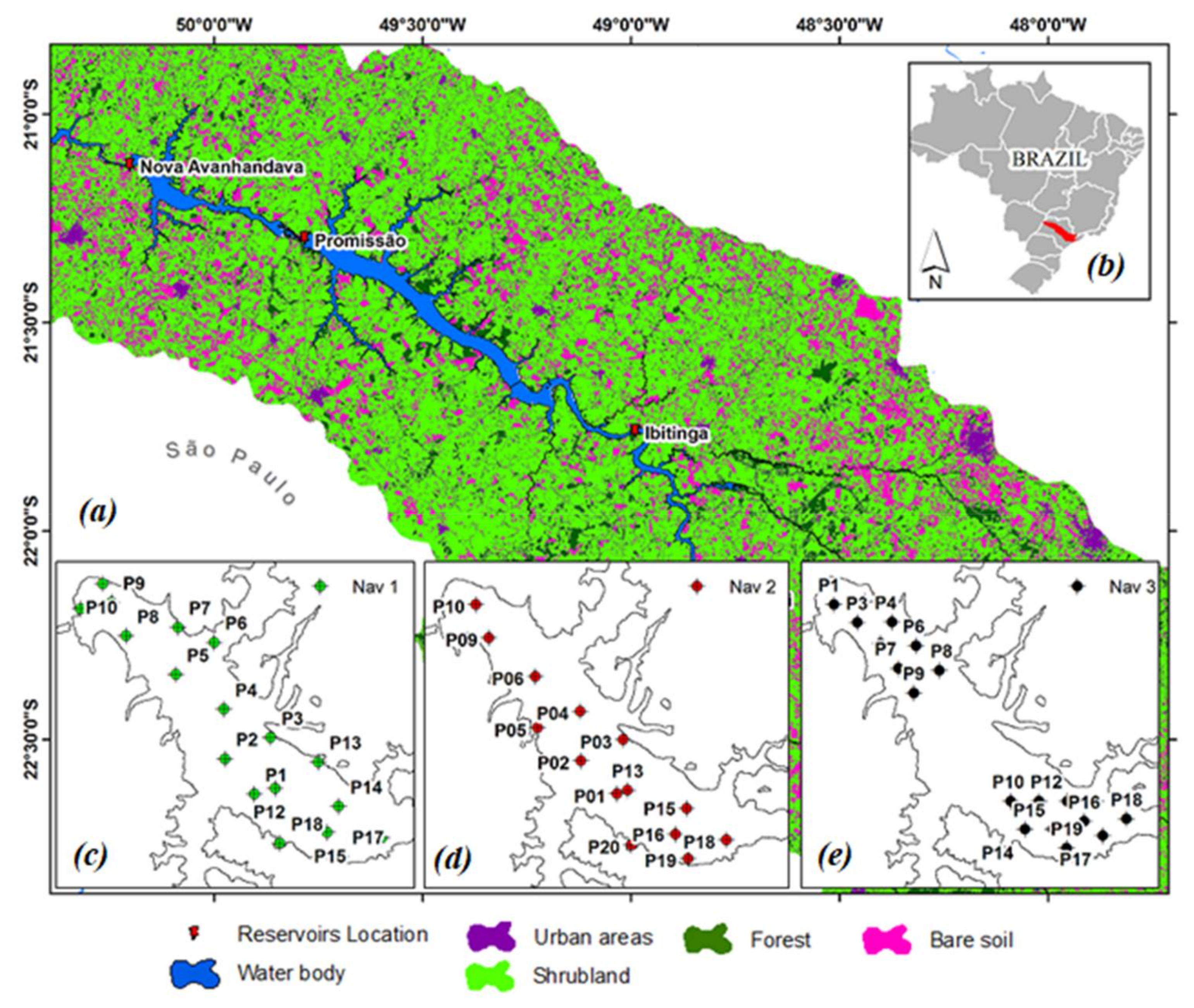
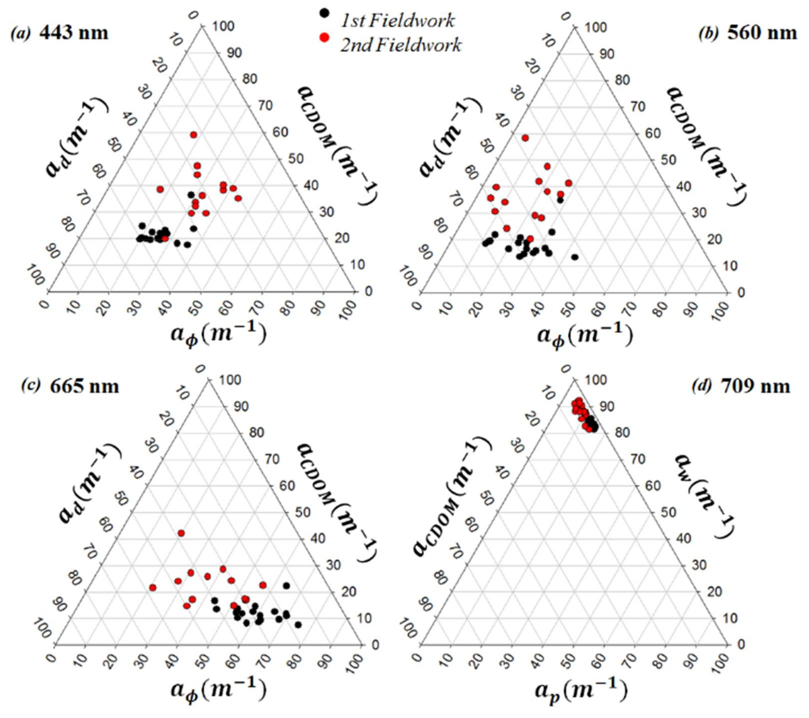
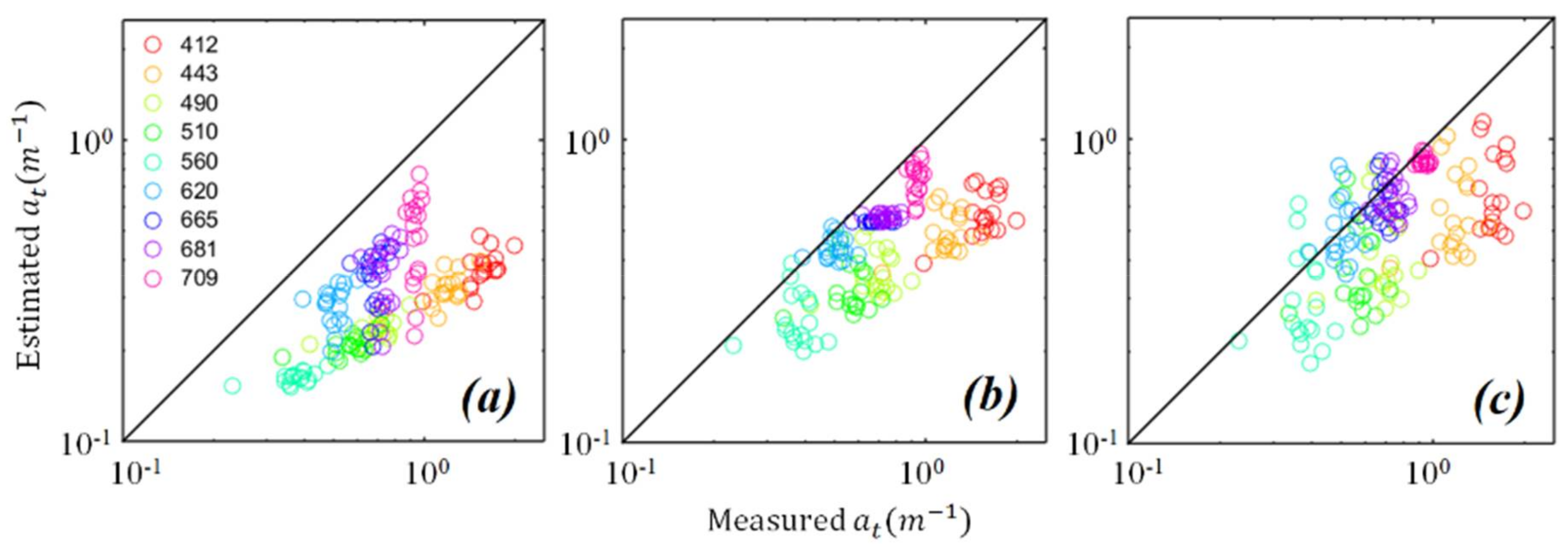
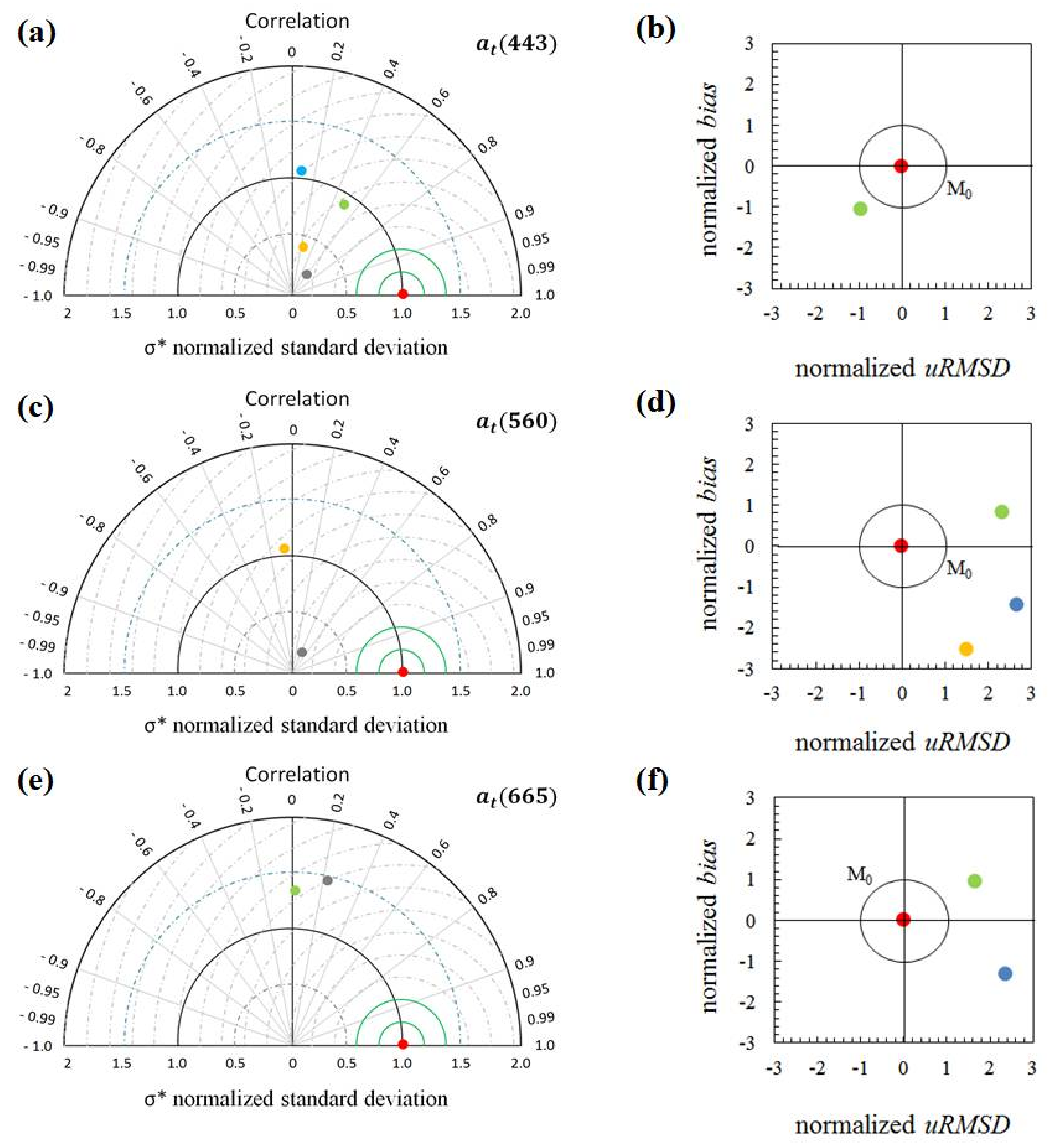
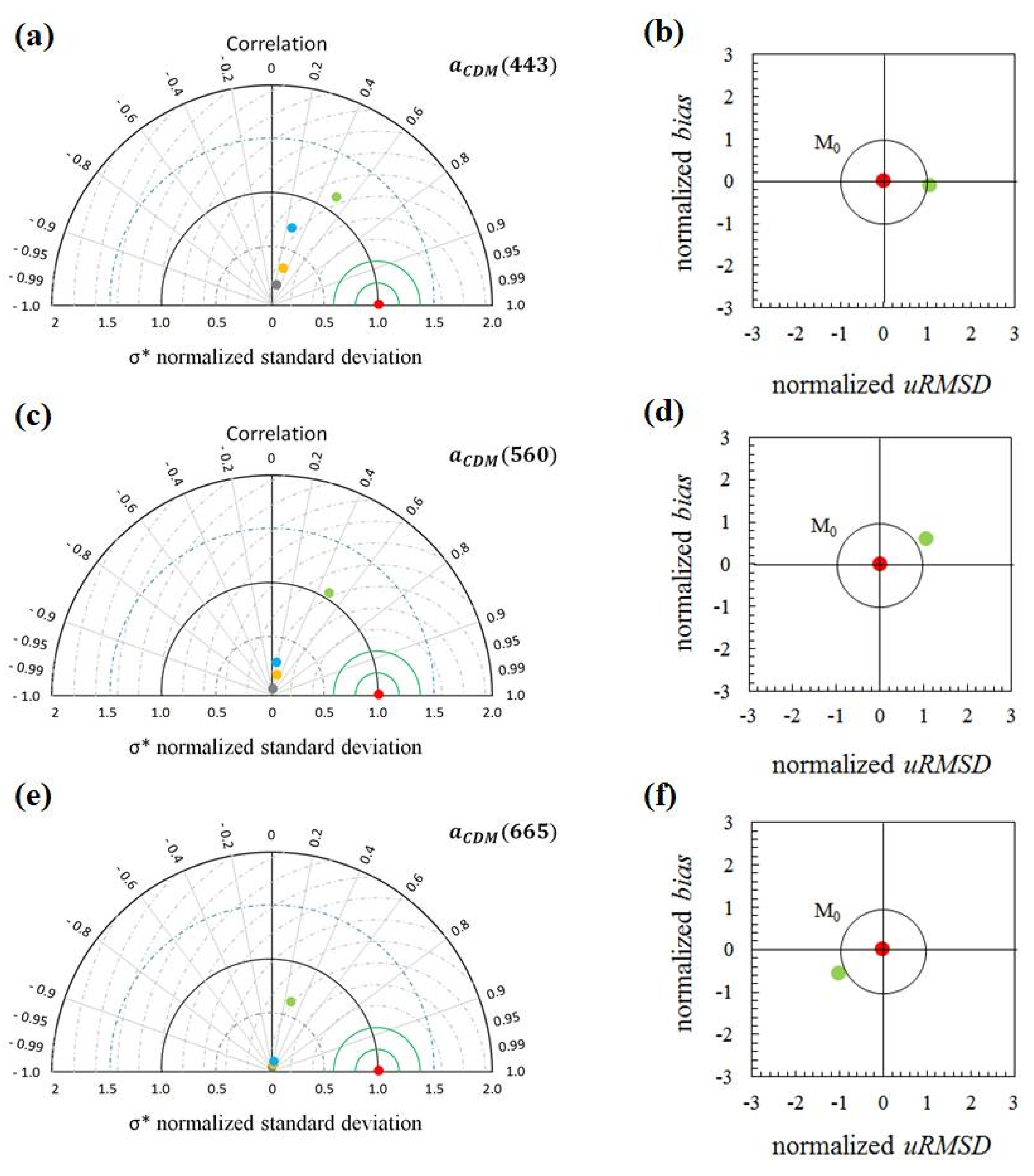
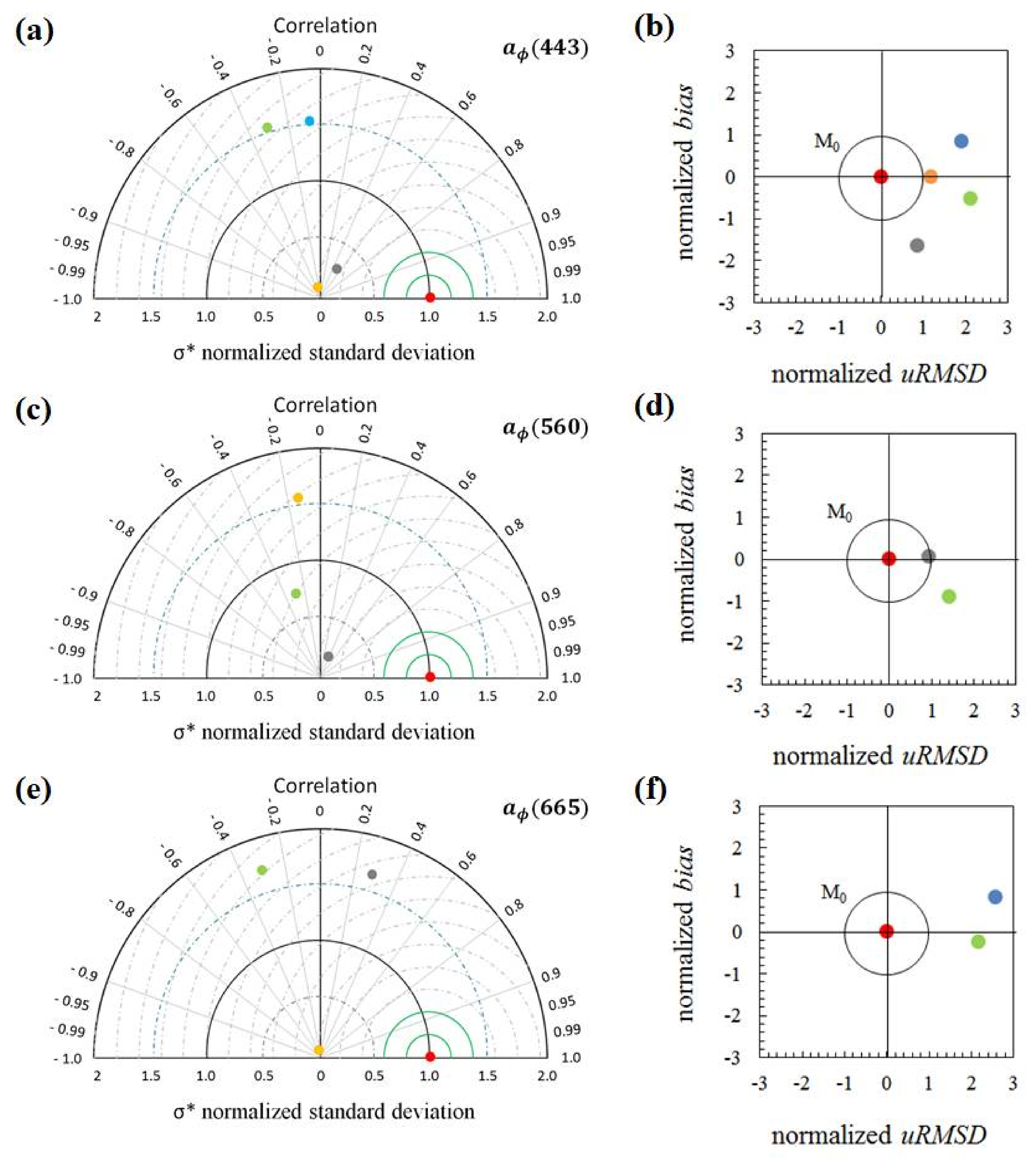
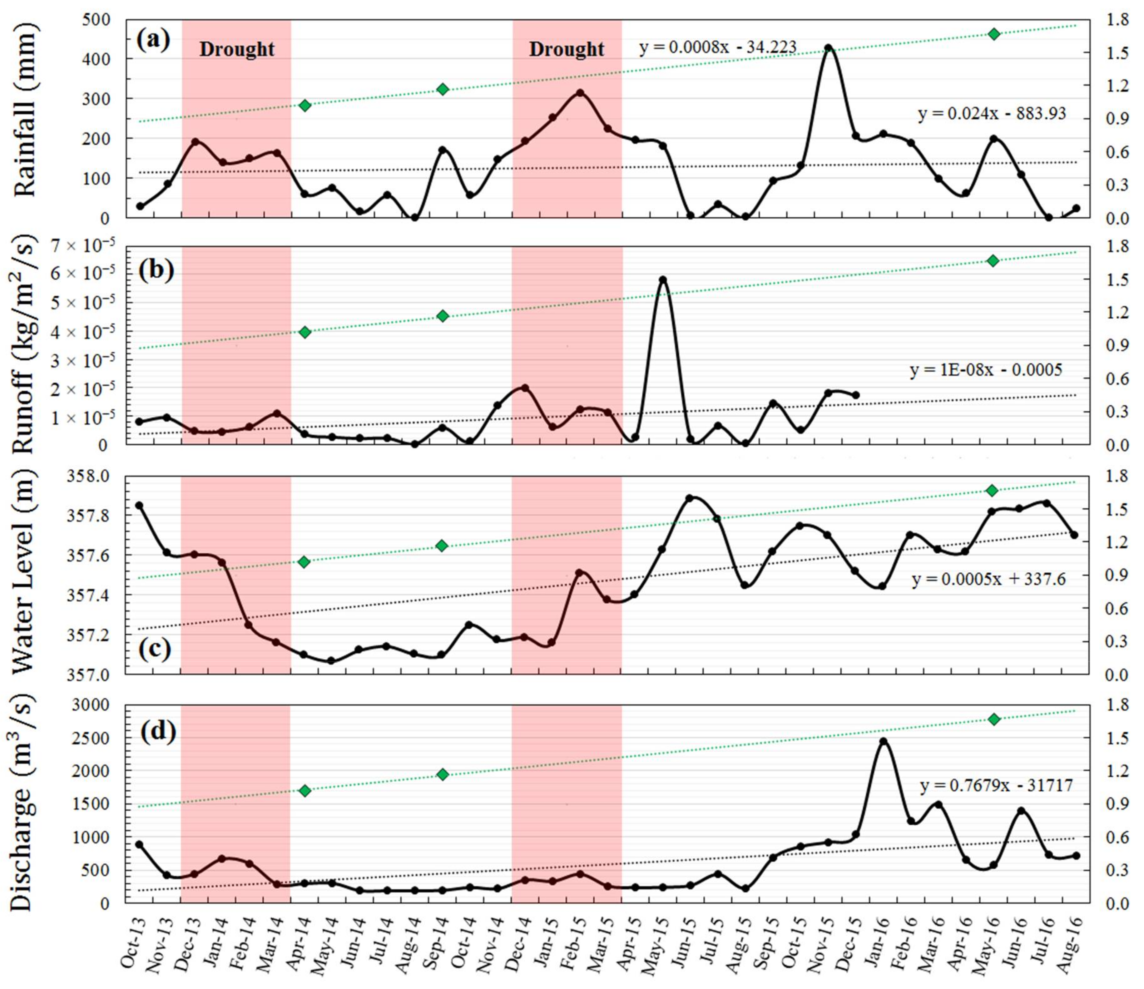
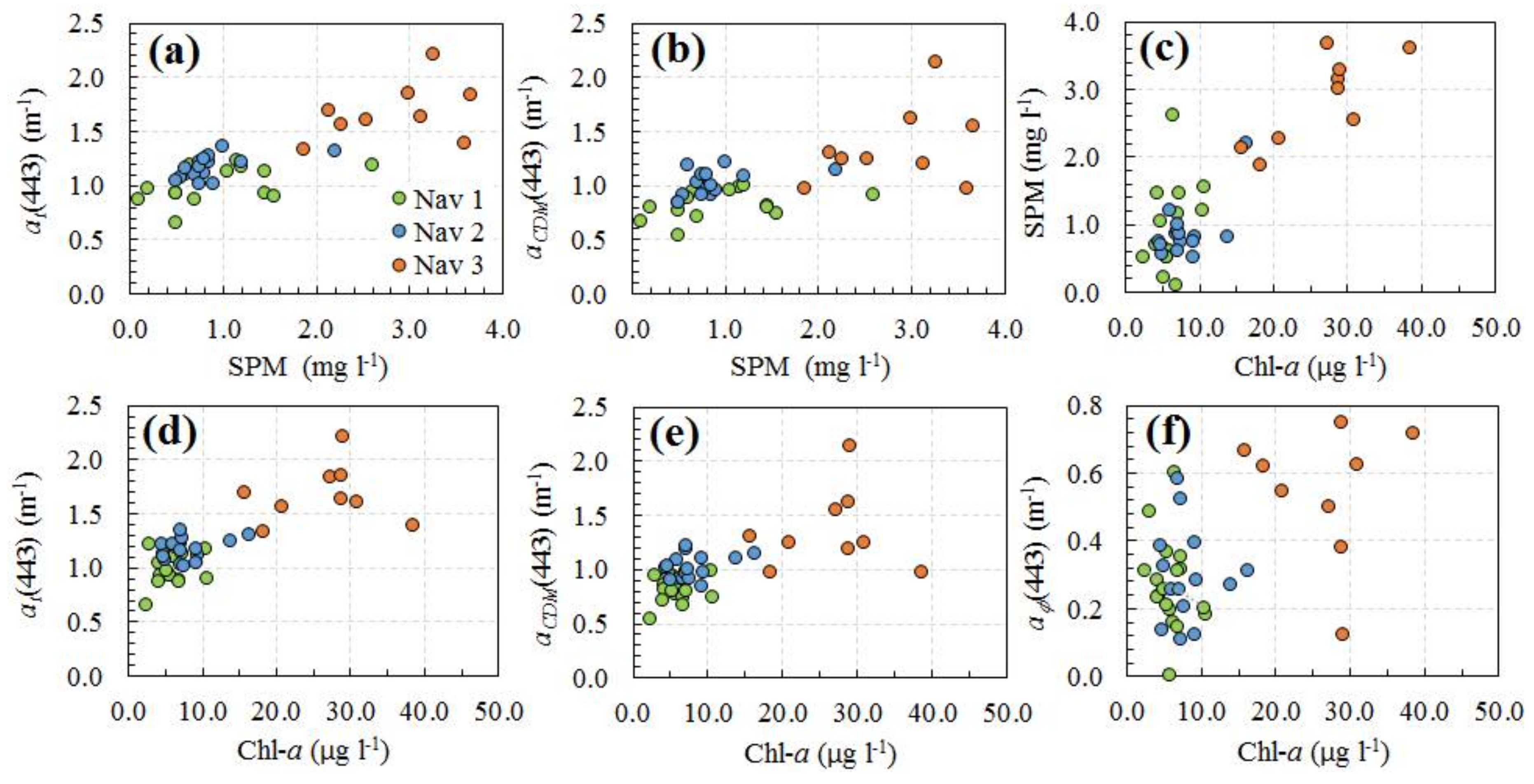
Table 1.
List of symbols and abbreviations.
| Symbol | Description | Unit |
|---|---|---|
| Absorption coefficient of pure water | m−1 | |
| Represented by the subtraction between | m−1 | |
| Absorption coefficient of detritus | m−1 | |
| Absorption coefficient of colored dissolved organic matter (CDOM) | m−1 | |
| Absorption coefficient of CDOM and detritus | m−1 | |
| Absorption coefficient of particulate matter | m−1 | |
| Absorption coefficient of phytoplankton | m−1 | |
| Total absorption coefficient, | m−1 | |
| Backscattering coefficient of pure water | m−1 | |
| Backscattering coefficient of particulate matter | m−1 | |
| Total backscattering coefficient, | m−1 | |
| Spectral power for backscattering coefficient | - | |
| Above-surface remote sensing reflectance | sr−1 | |
| Subsurface remote sensing reflectance | sr−1 | |
| Ratio of backscattering coefficient to the sum of backscattering and absorption coefficients | Unitless | |
| Spectral slope of colored detrital matter absorption coefficient | nm−1 | |
| - | ||
| - | ||
| Reference wavelength | nm |
Table 2.
Quasi-analytical algorithm (QAA) steps comparing version 5 from Lee et al. [20] and the QAAOMW proposed in this study.
Table 2.
Quasi-analytical algorithm (QAA) steps comparing version 5 from Lee et al. [20] and the QAAOMW proposed in this study.
| Property | QAALv5 | QAAOMW |
|---|---|---|
where | where | |
| — | ||
where | ||
Table 3.
Descriptive statistics of the water quality variables used for calibration and validation. SD is the standard deviation, CV is the coefficient of variation, and n is the number of samples.
Table 3.
Descriptive statistics of the water quality variables used for calibration and validation. SD is the standard deviation, CV is the coefficient of variation, and n is the number of samples.
| Average | SD | Minimum | Maximum | CV (%) | n | |
|---|---|---|---|---|---|---|
| April–May 2014 | ||||||
| (m−1) | 0.74 | 0.11 | 0.49 | 1.06 | 15.45 | 18 |
| (m−1) | 0.16 | 0.05 | 0.10 | 0.29 | 31.55 | 18 |
| (m−1) | 0.04 | 0.02 | 0.02 | 0.09 | 48.49 | 18 |
| (m−1) | 0.08 | 0.03 | 0.04 | 0.16 | 35.31 | 18 |
| (m−1) | 0.32 | 0.08 | 0.13 | 0.55 | 25.06 | 18 |
| (m−1) | 0.57 | 0.08 | 0.39 | 0.77 | 13.54 | 18 |
| SPM (mg L−1) | 0.95 | 0.63 | 0.10 | 2.60 | 66.04 | 15 |
| Chl-a (µg L−1) | 5.95 | 2.11 | 2.46 | 10.65 | 35.46 | 18 |
| Chl-a : SPM (µg/mg) | 12.27 | 15.97 | 2.47 | 68.26 | 130.14 | 15 |
| Depth (m) | 17.81 | 8.64 | 5.30 | 30.00 | 48.51 | 18 |
| Secchi depth (m) | 3.22 | 0.62 | 2.29 | 4.80 | 19.25 | 18 |
| Turbidity (NTU) | 1.60 | 0.41 | 1.01 | 2.47 | 25.35 | 18 |
| Zenital angle (DD) | 40.15 | 4.38 | 35.45 | 51.96 | 10.90 | 18 |
| Wind speed (m s−1) | 3.66 | 1.35 | 2.00 | 6.40 | 36.91 | 18 |
| September 2014 | ||||||
| (m−1) | 0.88 | 0.21 | 0.58 | 1.45 | 24.02 | 14 |
| (m−1) | 0.27 | 0.09 | 0.10 | 0.43 | 33.00 | 14 |
| (m−1) | 0.04 | 0.03 | 0.01 | 0.12 | 68.02 | 14 |
| (m−1) | 0.09 | 0.04 | 0.02 | 0.16 | 40.52 | 14 |
| (m−1) | 0.28 | 0.16 | 0.13 | 0.75 | 55.67 | 14 |
| (m−1) | 0.60 | 0.17 | 0.43 | 1.04 | 27.86 | 14 |
| SPM (mg L−1) | 0.93 | 0.42 | 0.50 | 2.20 | 45.21 | 13 |
| Chl-a (µg L−1) | 7.94 | 3.45 | 3.41 | 16.38 | 43.43 | 14 |
| Chl-a : SPM (µg/mg) | 9.83 | 4.23 | 4.75 | 18.57 | 43.05 | 13 |
| Depth (m) | 21.56 | 5.27 | 12.00 | 28.00 | 24.44 | 14 |
| Secchi depth (m) | 3.14 | 0.86 | 0.90 | 4.65 | 27.58 | 14 |
| Turbidity (NTU) | 2.44 | 2.46 | 1.01 | 11.17 | 100.97 | 14 |
| Zenital angle (DD) | 29.84 | 9.23 | 20.82 | 47.08 | 30.92 | 14 |
| Wind speed (m s−1) | 2.82 | 2.00 | 0.00 | 5.60 | 70.86 | 14 |
| May 2016 | ||||||
| (m−1) | 0.99 | 0.18 | 0.65 | 1.37 | 17.84 | 19 |
| (m−1) | 0.30 | 0.13 | 0.11 | 0.57 | 43.47 | 19 |
| (m-1) | 0.06 | 0.05 | 0.00 | 0.15 | 76.24 | 19 |
| (m−1) | 0.15 | 0.06 | 0.09 | 0.26 | 38.57 | 19 |
| (m−1) | 0.61 | 0.12 | 0.38 | 0.82 | 19.65 | 19 |
| (m−1) | 0.68 | 0.12 | 0.45 | 0.91 | 17.68 | 19 |
| SPM (mg L−1) | 3.08 | 0.94 | 1.87 | 5.30 | 30.69 | 10 |
| Chl-a (µg L−1) | 26.36 | 6.32 | 38.59 | 15.84 | 23.98 | 10 |
| Chl-a : SPM (µg/mg) | 8.93 | 1.96 | 4.64 | 12.21 | 21.95 | 10 |
| Depth (m) | - | |||||
| Secchi depth (m) | 2.97 | 0.63 | 1.91 | 3.80 | 21.03 | 19 |
| Turbidity (NTU) | - | |||||
| Zenital angle (DD) | 41.10 | 2.33 | 38.78 | 48.15 | 5.67 | 19 |
| Wind speed (m s−1) | 3.92 | 2.07 | 0.40 | 600 | 52.86 | 19 |
Table 4.
Comparative band-specific errors related to the re-parameterization of based on mean absolute percentage error (MAPE) (%) and root square mean difference (RSMD) (m−1) metrics. The first column represents the nominal OLCI center bands (nm).
Table 4.
Comparative band-specific errors related to the re-parameterization of based on mean absolute percentage error (MAPE) (%) and root square mean difference (RSMD) (m−1) metrics. The first column represents the nominal OLCI center bands (nm).
| OLCI Bands | QAALv5 | QAALv6 | QAAM14 | QAAOMW | ||||
|---|---|---|---|---|---|---|---|---|
| Wavelengths (nm) | RMSD (m−1) | MAPE (%) | RMSD (m−1) | MAPE (%) | RMSD (m−1) | MAPE (%) | RMSD (m−1) | MAPE (%) |
| 412 | 1.21 | 75.88 | 1.01 | 63.01 | 0.93 | 56.21 | 0.35 | 19.74 |
| 443 | 0.87 | 72.52 | 0.71 | 57.55 | 0.64 | 49.64 | 0.23 | 16.02 |
| 490 | 0.47 | 65.93 | 0.35 | 46.66 | 0.32 | 41.04 | 0.14 | 16.78 |
| 510 | 0.37 | 62.96 | 0.26 | 41.76 | 0.24 | 38.12 | 0.13 | 19.02 |
| 560 | 0.22 | 56.39 | 0.14 | 31.83 | 0.15 | 32.99 | 0.12 | 24.33 |
| 620 | 0.23 | 43.32 | 0.08 | 13.35 | 0.13 | 20.92 | 0.17 | 29.05 |
| 665 | 0.34 | 48.56 | 0.16 | 21.48 | 0.13 | 15.30 | 0.09 | 11.17 |
| 681 | 0.38 | 50.26 | 0.19 | 24.31 | 0.14 | 15.55 | 0.07 | 8.29 |
| 709 | 0.46 | 46.63 | 0.21 | 20.39 | 0.09 | 9.04 | 0.03 | 2.70 |
| Average | 0.51 | 58.05 | 0.35 | 35.59 | 0.31 | 30.98 | 0.15 | 16.35 |
Table 5.
Comparative band-specific errors related to the re-parameterization of based on MAPE (%) and RSMD (m−1) metrics. The first column represents the nominal OLCI center bands (nm).
Table 5.
Comparative band-specific errors related to the re-parameterization of based on MAPE (%) and RSMD (m−1) metrics. The first column represents the nominal OLCI center bands (nm).
| OLCI Bands | QAALv5 | QAALv6 | QAAM14 | QAAOMW | ||||
|---|---|---|---|---|---|---|---|---|
| Wavelengths (nm) | RMSD (m−1) | MAPE (%) | RMSD (m−1) | MAPE (%) | RMSD (m−1) | MAPE (%) | RMSD (m−1) | MAPE (%) |
| 412 | 1.03 | 81.35 | 0.96 | 75.81 | 0.93 | 72.88 | 0.21 | 12.76 |
| 443 | 0.74 | 83.90 | 0.69 | 79.13 | 0.67 | 76.61 | 0.13 | 12.99 |
| 490 | 0.47 | 87.77 | 0.45 | 84.14 | 0.44 | 82.22 | 0.08 | 14.68 |
| 510 | 0.38 | 89.06 | 0.37 | 85.81 | 0.36 | 84.09 | 0.07 | 15.57 |
| 560 | 0.22 | 91.53 | 0.21 | 89.02 | 0.21 | 87.70 | 0.04 | 17.98 |
| 620 | 0.13 | 94.28 | 0.12 | 92.61 | 0.12 | 91.74 | 0.03 | 19.92 |
| 665 | 0.10 | 96.48 | 0.10 | 95.45 | 0.10 | 94.89 | 0.03 | 21.04 |
| 681 | 0.10 | 97.15 | 0.09 | 96.31 | 0.09 | 95.86 | 0.03 | 24.18 |
| 709 | 0.08 | 97.89 | 0.08 | 97.27 | 0.08 | 96.93 | 0.03 | 30.66 |
| Average | 0.36 | 91.05 | 0.34 | 88.39 | 0.33 | 86.99 | 0.07 | 18.87 |
Table 6.
Comparative band-specific errors related to the re-parameterization of based on MAPE (%) and RSMD (m−1) metrics. The first column represents the nominal OLCI center bands (nm).
Table 6.
Comparative band-specific errors related to the re-parameterization of based on MAPE (%) and RSMD (m−1) metrics. The first column represents the nominal OLCI center bands (nm).
| OLCI Bands | QAALv5 | QAALv6 | QAAM14 | QAAOMW | ||||
|---|---|---|---|---|---|---|---|---|
| Wavelengths (nm) | RMSD (m−1) | MAPE (%) | RMSD (m−1) | MAPE (%) | RMSD (m−1) | MAPE (%) | RMSD (m−1) | MAPE (%) |
| 412 | 0.19 | 53.69 | 0.11 | 21.31 | 0.14 | 33.80 | 0.19 | 44.39 |
| 443 | 0.15 | 40.10 | 0.10 | 25.20 | 0.17 | 45.24 | 0.18 | 42.67 |
| 490 | 0.04 | 24.02 | 0.14 | 92.11 | 0.22 | 130.02 | 0.10 | 47.57 |
| 510 | 0.04 | 34.77 | 0.16 | 150.98 | 0.22 | 184.86 | 0.08 | 47.97 |
| 560 | 0.03 | 42.49 | 0.16 | 238.37 | 0.18 | 229.39 | 0.05 | 47.28 |
| 620 | 0.11 | 100.73 | 0.33 | 402.82 | 0.19 | 173.98 | 0.06 | 45.56 |
| 665 | 0.25 | 157.52 | 0.37 | 264.71 | 0.11 | 56.92 | 0.09 | 46.47 |
| 681 | 0.29 | 167.75 | 0.38 | 241.91 | 0.10 | 42.84 | 0.10 | 46.04 |
| 709 | 0.38 | 870.85 | 0.69 | 1858.15 | 0.04 | 63.91 | 0.04 | 53.29 |
| Average | 0.16 | 165.77 | 0.27 | 366.17 | 0.15 | 106.77 | 0.10 | 46.80 |
Table 7.
Comparative band-specific errors after validation procedure of , , and based on MAPE (%) and RSMD (m−1) metrics. The first column represents the nominal OLCI center bands (nm).
Table 7.
Comparative band-specific errors after validation procedure of , , and based on MAPE (%) and RSMD (m−1) metrics. The first column represents the nominal OLCI center bands (nm).
| OLCI Bands | ||||||
|---|---|---|---|---|---|---|
| Wavelengths (nm) | RMSD (m−1) | MAPE (%) | RMSD (m−1) | MAPE (%) | RMSD (m−1) | MAPE (%) |
| 412 | 0.43 | 36.00 | 0.56 | 66.21 | 0.14 | 41.23 |
| 443 | 0.36 | 41.40 | 0.44 | 78.30 | 0.13 | 39.27 |
| 490 | 0.30 | 57.66 | 0.28 | 79.34 | 0.08 | 46.24 |
| 510 | 0.26 | 59.74 | 0.22 | 73.89 | 0.05 | 44.65 |
| 560 | 0.20 | 62.81 | 0.12 | 58.89 | 0.03 | 85.02 |
| 620 | 0.26 | 54.15 | 0.05 | 30.95 | 0.04 | 176.35 |
| 665 | 0.16 | 22.81 | 0.04 | 19.37 | 0.08 | 94.12 |
| 681 | 0.10 | 12.65 | 0.05 | 26.54 | 0.08 | 70.31 |
| 709 | 0.05 | 4.15 | 0.05 | 35.82 | - | - |
| Average | 0.23 | 39.04 | 0.20 | 52.15 | 0.08 | 74.65 |
© 2018 by the authors. Licensee MDPI, Basel, Switzerland. This article is an open access article distributed under the terms and conditions of the Creative Commons Attribution (CC BY) license (http://creativecommons.org/licenses/by/4.0/).
Share and Cite
MDPI and ACS Style
Rodrigues, T.; Mishra, D.R.; Alcântara, E.; Astuti, I.; Watanabe, F.; Imai, N. Estimating the Optical Properties of Inorganic Matter-Dominated Oligo-to-Mesotrophic Inland Waters. Water 2018, 10, 449. https://doi.org/10.3390/w10040449
AMA Style
Rodrigues T, Mishra DR, Alcântara E, Astuti I, Watanabe F, Imai N. Estimating the Optical Properties of Inorganic Matter-Dominated Oligo-to-Mesotrophic Inland Waters. Water. 2018; 10(4):449. https://doi.org/10.3390/w10040449
Chicago/Turabian StyleRodrigues, Thanan, Deepak R. Mishra, Enner Alcântara, Ike Astuti, Fernanda Watanabe, and Nilton Imai. 2018. "Estimating the Optical Properties of Inorganic Matter-Dominated Oligo-to-Mesotrophic Inland Waters" Water 10, no. 4: 449. https://doi.org/10.3390/w10040449
Note that from the first issue of 2016, this journal uses article numbers instead of page numbers. See further details here.